WWW.NATURE.COM/NATURE | 1 SUPPLEMENTARY INFORMATION doi:10.1038/nature14272 1. Supplementary Methods Sections: 1. Methods summary 2. Glass slide preparation 3. Chemicals 4. Droplet spreading 5. Devices 6. Reflectometry 2. Internal flow 3. Long-range attraction 4. Short-range chasing fluid exchange 5. Devices 6. Self-sorting device 7. Repulsive long-range positioning 8. Parallel plate devices 9. Easy way to recreate 4. Supplementary References References cited only in Supplementary Information 7. Humidity chamber experiments 8. Flow visualization 9. Long-range phase plot 10. Short-range phase plot 11. Measurement of drag 2. Supplementary Discussion Sections: 1. Drag coefficient theory 2. Comparison of experimental drag coefficient with theory 3. Flux-based contact angle model 4. Model for long-range interactions 5. Assessment of thermocapillarity Contents: 3. Supplementary Videos 1. Long-range and short-range interactions in two-component droplets
Transcript
w w w. n a t u r e . c o m / n a t u r e | 1
SuPPLementarY InFormatIondoi:10.1038/nature14272
1
Supplementary information:
Contents:
1. Supplementary Methods
Sections:
1. Methods summary
2. Glass slide preparation
3. Chemicals
4. Droplet spreading
5. Devices
6. Reflectometry
7. Humidity chamber experiments
8. Flow visualization
9. Long-range phase plot
10. Short-range phase plot
11. Measurement of drag
2. Supplementary Discussion
Sections:
1. Drag coefficient theory
2. Comparison of experimental drag coefficient with theory
3. Flux-based contact angle model
4. Model for long-range interactions
5. Assessment of thermocapillarity
3. Supplementary Videos
1. Long-range and short-range interactions in two-component droplets
2
2. Internal flow
3. Long-range attraction
4. Short-range chasing fluid exchange
5. Devices
6. Self-sorting device
7. Repulsive long-range positioning
8. Parallel plate devices
9. Easy way to recreate
4. Supplementary References
References cited only in Supplementary Information
1
Supplementary information:
Contents:
1. Supplementary Methods
Sections:
1. Methods summary
2. Glass slide preparation
3. Chemicals
4. Droplet spreading
5. Devices
6. Reflectometry
7. Humidity chamber experiments
8. Flow visualization
9. Long-range phase plot
10. Short-range phase plot
11. Measurement of drag
2. Supplementary Discussion
Sections:
1. Drag coefficient theory
2. Comparison of experimental drag coefficient with theory
3. Flux-based contact angle model
4. Model for long-range interactions
5. Assessment of thermocapillarity
3. Supplementary Videos
1. Long-range and short-range interactions in two-component droplets
SUPPLEMENTARY INFORMATION
2 | w w w. n a t u r e . c o m / n a t u r e
RESEARCH
3
1. Supplementary methods:
1. Methods summary: Glass slides (Pearl Microscope Slides NO. 7101) taken directly from the box were treated for 1 minute using a handheld corona discharge (Electro-Technic BD-20AC) and used within 5 minutes of treatment. Chemicals were obtained from Sigma Aldrich, or as a gift from Graham Dick as listed below. They were mixed in volume/total volume percentages, unless otherwise noted (see list below). The contact angle was measured with the reflectometry method described by Allain et al.33. Humidity controlled experiments were conducted in a sealed chamber with saturated salt solutions controlling the humidity. Flow visualization was performed using fluorescent polystyrene beads (Polyscience fluoresbrite, “Polychro red” size 5 μm, 2 µm, and 1.095 µm. The measurement of drag as a function of velocity was done by depositing droplets on ramps of known angle and filming from the top.
2. Glass slide preparation: Unless otherwise stated, substrates were prepared and used as follows: Soda-lime glass slides (Pearl Microscope Slides NO. 7101) taken directly from the box were treated for 1 minute using a handheld corona discharge (Electro-Technic BD-20AC) and used within 5 minutes of treatment. We found that droplet behaviour was sensitive to ambient air currents and we used a clear box to shield experiments from these disturbances. We found that the droplet behaviour was not sensitive to glass type or quality or exact parameters of corona treatment. Images and videos were obtained using a Canon 5D Mark II camera (30 fps). Food colouring (McCormick) was used to aid visualization in videos and images, but not in quantitative experiments. Before use, the food colouring was first evaporated over several days at 60 ºC in tubes on a hot plate and this powder added to mixtures of known concentrations (to minimize any solvent contamination).
Other clean high energy substrates can also be used. We found that cleaning glass with a Bunsen burner flame for 20-30 s or cleaning glass with a piranha solution also worked. Additionally we noticed similar effects on the flexible substrate indium tin oxide coated polyethylene terephthalate (Sigma Aldrich, product number: 639303) which we treated for 5 min in a plasma oven (Harrick Plasma, Plasma cleaner). Clean flamed aluminium can also be used as a substrate.
3. Chemicals: Chemicals were obtained from Sigma Aldrich, or as a gift from Graham Dick as listed below. They were mixed in volume/total volume percentages, unless otherwise noted.
propylene glycol (PG) (Sigma Aldrich), water (Sigma Aldrich), tripropylene glycol (TPG) (Sigma Aldrich), 1,3-butanediol (Sigma Aldrich), ethanolamine (gift from Graham Dick), glycerol (Sigma Aldrich), ethylene glycol (Sigma Aldrich), dimethyl sulfoxide (Sigma Aldrich), p-dioxane (Sigma Aldrich), dipropylene glycol methyl ether (DPGME) (Sigma Aldrich), acetic acid (Sigma Aldrich), acetone (Sigma Aldrich), ethanol (Sigma Aldrich), methanol (Sigma Aldrich), isopropanol (IPA) (Sigma Aldrich), 1-propanol (Sigma Aldrich), pyridine (gift from Graham Dick), formic acid (Sigma Aldrich), furfuryl alcohol (Sigma Aldrich), morpholine (gift from Graham Dick), dimethylformamide (DMF) (gift from Graham Dick)
w w w. n a t u r e . c o m / n a t u r e | 3
SUPPLEMENTARY INFORMATION RESEARCH
4
4. Droplet spreading: We tested all possible two-component liquid mixtures for spreading or droplet formation in a library of 21 miscible chemicals (Extended Data Table 1). Chemical components were selected to have a wide range of vapour pressures and surface tensions. We mixed chemicals in equal volume ratios and placed a 0.5 μL droplet of each mixture on a corona treated clean glass slide, then observed the droplet behaviour. Mixtures where one chemical had both higher surface tension and higher vapour pressure formed droplets which had characteristics of the PG/water droplets characterized in detail here (Fig. 2c), while mixtures where one component had lower vapour pressure but higher surface tension spread rapidly. Mixtures where the chemicals have either similar surface tensions or vapour pressures were less predictable. 5. Devices: Hydrophobic patterns were drawn using thin and thick tipped permanent markers (Sharpie™) both by hand and by programming an automated plotter/cutter (Roland Camm1-Servo). The patterns on the glass slides were reusable. We found that slides with patterns could be rinsed with distilled water, dried with nitrogen, and retreated at least several times without noticeable changes in behaviour.
6. Reflectometry: A contact angle measurement setup was created according to Allain et al. 33. Reflectometry involves using the droplet as a convex mirror to reflect collimated light up onto a screen where the diameter of the reflection can be measured and contact angle determined from the geometries of the setup. The setup we created could image contact angles roughly from 1 to 45 degrees with a reproducibility of ± 0.25 degrees. Droplet contact angles were measured immediately after deposition to minimize any change in concentration from evaporation of the bulk droplet. We did not notice any effects from local heating of the laser.
7. Humidity chamber experiments: Saturated salt solutions were used to control relative humidity. In practice we placed 4 small weigh boats containing saturated salt solution and a treated glass slide into large (140 mm diameter, 15 mm height) petri dishes sealed with parafilm. We waited 1 hour before introducing droplets and measuring contact angles (by reflectometry) to allow the relative humidity to equilibrate (measurements with an electronic humidity sensor indicated that humidity was stable in these chambers after 30 min). Droplets were introduced through a small hole drilled in the lid of the dish which was only uncovered briefly for introduction of the droplet. The droplet contact angle was measured immediately after deposition.
8. Flow visualization: Fluorescent polystyrene beads (Polyscience fluoresbrite, “Polychro red” size 5 μm, 2 µm, and 1.095 µm) were introduced into droplets to visualize flows. We used an Orca4 CMOS camera (Hamamatsu) on a Nikon AZ100 stereoscope to capture these flow patterns with a frame rate of 50 fps. We captured three dimensional flow patterns as shown in Fig. 2e on the same setup by zooming and adjusting the focal plane such that the beads only at the bottom or top of the droplet were in focus.
SUPPLEMENTARY INFORMATION
4 | w w w. n a t u r e . c o m / n a t u r e
RESEARCH
5
9. Long-range phase plot: The phase plot in Fig. 3c was created by setting two droplets of different concentration around one diameter apart. One droplet was pinned by placing it behind a thin hydrophobic sharpie line and the other free to move. We recorded the direction of motion of the mobile droplet (attraction or repulsion). We noticed no difference between this method of pinning and pinning the droplets using a break in the substrate.
10. Short-range phase plot: The phase plot in Extended Data Fig. 8 was created by setting two PG/water droplets near each other on a treated slide and varying the droplet concentrations. The qualitative behaviour of the two droplets after contact was recorded. We found these short-range interactions could be classified into four different types. 1) If the concentration was similar (little surface tension difference) the droplets coalesced (merge). 2) If one droplet had very high PG %, then it tended to form a thin tendril which reached out and chased the other droplet without detaching from the back droplet. We also observed chasing 3) where the back droplet was intact and 4) where the back droplet broke into two droplets of unequal size, and the smaller ‘satellite’ droplet did the chasing. Different phase plots can be achieved by changing droplet volume either by increasing or decreasing the volumes of both droplets in the same way, or by choosing different droplet volumes.
11. Measurement of drag: We constructed a ramp with adjustable slope to measure the drag on moving droplets. We adjusted the angle of the ramp 𝛼𝛼 (calculated by measuring side lengths and using trigonometry) to obtain a driving force 𝑚𝑚𝑚𝑚sin(𝛼𝛼) parallel to the ramp with 𝑚𝑚 the mass of the droplet and 𝑚𝑚 the gravitational acceleration. At terminal velocity (reached much faster than 1 s) the drag force is equal to the driving force, and we obtain the drag force as a function of velocity.
2. Supplementary discussion
1. Drag coefficient theory:
Following Brochard34, the viscous drag in a droplet of small contact angle occurs mainly at the contact line where the shear gradient is the sharpest. The drag force per unit length of a contact line moving perpendicularly at a velocity 𝑈𝑈 is given by 𝐹𝐹drag = 3𝜂𝜂𝜂𝜂𝑙𝑙n
𝜃𝜃 with 𝜃𝜃 being the contact
angle, 𝜂𝜂 the dynamic viscosity, and cutoff constant, 𝑙𝑙n = ln 𝑥𝑥max𝑥𝑥min
with 𝑥𝑥max and 𝑥𝑥min as the two
cutoff lengths, typically 𝑥𝑥max = 𝑅𝑅 the radius of the droplet, and 𝑥𝑥min is on the order of the molecular size of the liquid, usually 𝑙𝑙n is between 10 and 15.
In the present case, as the droplet moves at the velocity, 𝑈𝑈, the apparent contact line between the bulk droplet and the thin film moves at the velocity 𝑈𝑈sin(𝜓𝜓), with 𝜓𝜓 as the angle to the direction of propagation. Integrating the drag force around the droplet one finds the total drag on the droplet:
w w w. n a t u r e . c o m / n a t u r e | 5
SUPPLEMENTARY INFORMATION RESEARCH
6
𝐹𝐹drag = 3𝜋𝜋𝜋𝜋𝜋𝜋𝜋𝜋𝑙𝑙n𝜃𝜃 .
The velocity as a function of the driving force measurements are represented in Extended Data Fig. 6 for 10% PG droplets of various volumes. We observe that the drag force linearly increases with the velocity and that it increases with the droplet’s volume.
As the droplet is submitted to gravitational acceleration on a ramp of angle 𝛼𝛼, the force equilibrium in the direction of movement is written as:
3𝜋𝜋𝜋𝜋𝜋𝜋𝜋𝜋𝑙𝑙n𝜃𝜃 = 𝑚𝑚𝑚𝑚sin(𝛼𝛼).
Thus the rescaled velocity of the droplet is written as:
𝜋𝜋𝜋𝜋max
= sin (𝛼𝛼),
with 𝑈𝑈max = 𝜃𝜃𝜃𝜃𝜃𝜃3𝜋𝜋𝜋𝜋𝑙𝑙n𝜋𝜋 being the theoretical velocity of the droplet on a vertical plane. We observe
that the data for 5 different sizes of droplet coincide well with the theoretical prediction for 𝑙𝑙n = 11.2 as seen in Extended Data Fig. 7.
2. Comparison of experimental drag coefficient with theory
Here we compare our experimental results of drag on a droplet with the analytical model proposed by Brochard. From the experiments in ‘Measurement of drag’ for a 0.5 µl droplet of 10% PG, the drag coefficient 𝐶𝐶drag is 1.94 mm
s∗μN. The theoretical drag coefficient is given by
𝐶𝐶drag = 3𝜋𝜋𝜋𝜋𝜋𝜋𝜋𝜋𝑙𝑙n𝜃𝜃 = 1.97 mm
s∗μN (for 𝜂𝜂 = 3.13 ∗ 10−3 Pa ∗ s, from literature35, 𝜃𝜃 = 0.24 radians, as
measured on the day of data collection, 𝑟𝑟 = 1.39 mm, calculated by assuming a spherical cap using the volume 0.5 μL and measured contact angle, 𝑙𝑙n=11.2) and agrees well with the observations.
Though this theory was developed for a moving three-phase contact line it works remarkably well even in this case where the droplet is surrounded by a thin film.
SUPPLEMENTARY INFORMATION
6 | w w w. n a t u r e . c o m / n a t u r e
RESEARCH
7
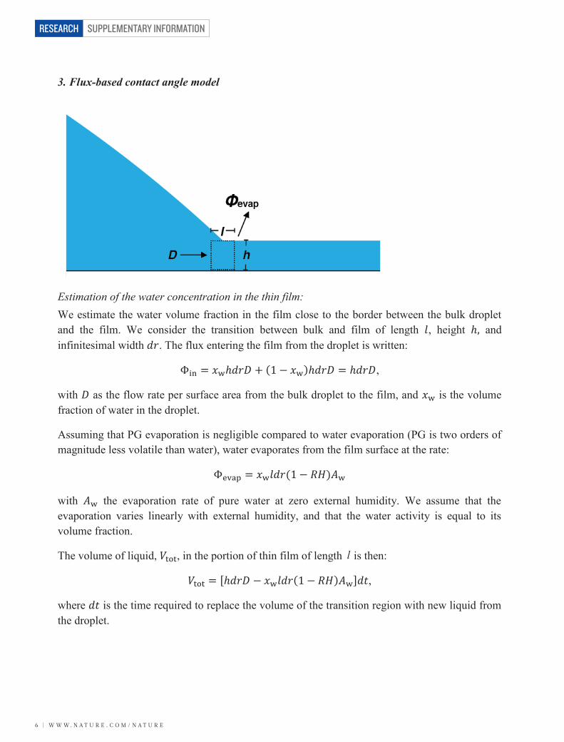
3. Flux-based contact angle model
Estimation of the water concentration in the thin film: We estimate the water volume fraction in the film close to the border between the bulk droplet and the film. We consider the transition between bulk and film of length 𝑙𝑙, height ℎ, and infinitesimal width 𝑑𝑑𝑑𝑑. The flux entering the film from the droplet is written:
Φin = 𝑥𝑥wℎ𝑑𝑑𝑑𝑑𝑑𝑑 + (1 − 𝑥𝑥w)ℎ𝑑𝑑𝑑𝑑𝑑𝑑 = ℎ𝑑𝑑𝑑𝑑𝑑𝑑,
with 𝑑𝑑 as the flow rate per surface area from the bulk droplet to the film, and 𝑥𝑥w is the volume fraction of water in the droplet.
Assuming that PG evaporation is negligible compared to water evaporation (PG is two orders of magnitude less volatile than water), water evaporates from the film surface at the rate:
Φevap = 𝑥𝑥w𝑙𝑙𝑑𝑑𝑑𝑑(1 − 𝑅𝑅𝑅𝑅)𝐴𝐴w
with 𝐴𝐴w the evaporation rate of pure water at zero external humidity. We assume that the evaporation varies linearly with external humidity, and that the water activity is equal to its volume fraction.
The volume of liquid, 𝑉𝑉tot, in the portion of thin film of length is then:
𝑉𝑉tot = [ℎ𝑑𝑑𝑑𝑑𝑑𝑑 − 𝑥𝑥w𝑙𝑙𝑑𝑑𝑑𝑑(1 − 𝑅𝑅𝑅𝑅)𝐴𝐴w]𝑑𝑑𝑑𝑑,
where 𝑑𝑑𝑑𝑑 is the time required to replace the volume of the transition region with new liquid from the droplet.
l
w w w. n a t u r e . c o m / n a t u r e | 7
SUPPLEMENTARY INFORMATION RESEARCH
8
The volume fraction of water in the thin film (𝑥𝑥wfilm) assuming dimensions of the transition region do not change over time, and the water fraction changes only a small amount over this region is:
With 𝐾𝐾 = 𝐴𝐴w𝑙𝑙ℎ𝑑𝑑 , we can rewrite the above equation as:
𝑥𝑥wfilm = 𝑥𝑥w[1−𝐾𝐾(1−𝑅𝑅𝑅𝑅)]1−𝑥𝑥w(1−𝑅𝑅𝑅𝑅)𝐾𝐾
.
The predicted film water concentration is close to the droplet water concentration for large and small water volume fractions, and smaller at intermediate values, as presented in Extended Data Fig.4.
From the film composition we estimate the film surface tension (as explained below in ‘Surface tension of the two-component mixture’) and deduce the droplet contact angle using:
cos(𝜃𝜃app) =𝛾𝛾LVfilm
𝛾𝛾LVdroplet.
Fixing 𝐾𝐾 = 0.4 (fit at 40% RH) we observe that the model captures the contact angle as a function of the initial mixture composition, at two different relative humidities (Fig. 2a).
Surface tension of the two-component mixture: The surface tension of propylene glycol/water two-component mixtures is given by Karpitschka and Riegler36.
We fit the data in the above paper with a fourth order polynomial:
Here is the water mass fraction, which we converted to volume fraction using the densities.
Contact angle as a function of external humidity:
For a 10% PG droplet, the film water fraction as a function of humidity is plotted in Extended Data Fig. 5. The film composition model predicts a film composition between 80% and 90% water for an external humidity varying from 0 to 100 %. In this range the surface tension of the two-component mixture is well approximated with a linear relation:
𝛾𝛾LV = 66.4𝑥𝑥w + 2.1.
In the range 𝑅𝑅𝑅𝑅 = [0.1, 1] the film water volume fraction can also be fit by a linear relation:
x
SUPPLEMENTARY INFORMATION
8 | w w w. n a t u r e . c o m / n a t u r e
RESEARCH
9
𝑥𝑥wfilm = 5.2 × 10⁻²𝑅𝑅𝑅𝑅 + 0.851
The droplet cosine of the contact angle is thus estimated to vary linearly with the external humidity, in agreement with the observations.
Theoretically we predict the cosine of the contact angle to be:
cos(𝜃𝜃) = 𝛾𝛾LVfilm𝛾𝛾LVdroplet
= 5.57 × 10⁻²𝑅𝑅𝑅𝑅 + 0.944.
While the experimental fit is:
cos(𝜃𝜃) = 𝛾𝛾LVfilm𝛾𝛾LVdroplet
= 2.5 × 10⁻²𝑅𝑅𝑅𝑅 + 0.963,
showing a reasonable agreement between the evaporation model and the experiments. Note, here we have assumed flux due to flow into the thin film, however we could exchange flow for diffusion in our model and obtain similar results.
w w w. n a t u r e . c o m / n a t u r e | 9
SUPPLEMENTARY INFORMATION RESEARCH
10
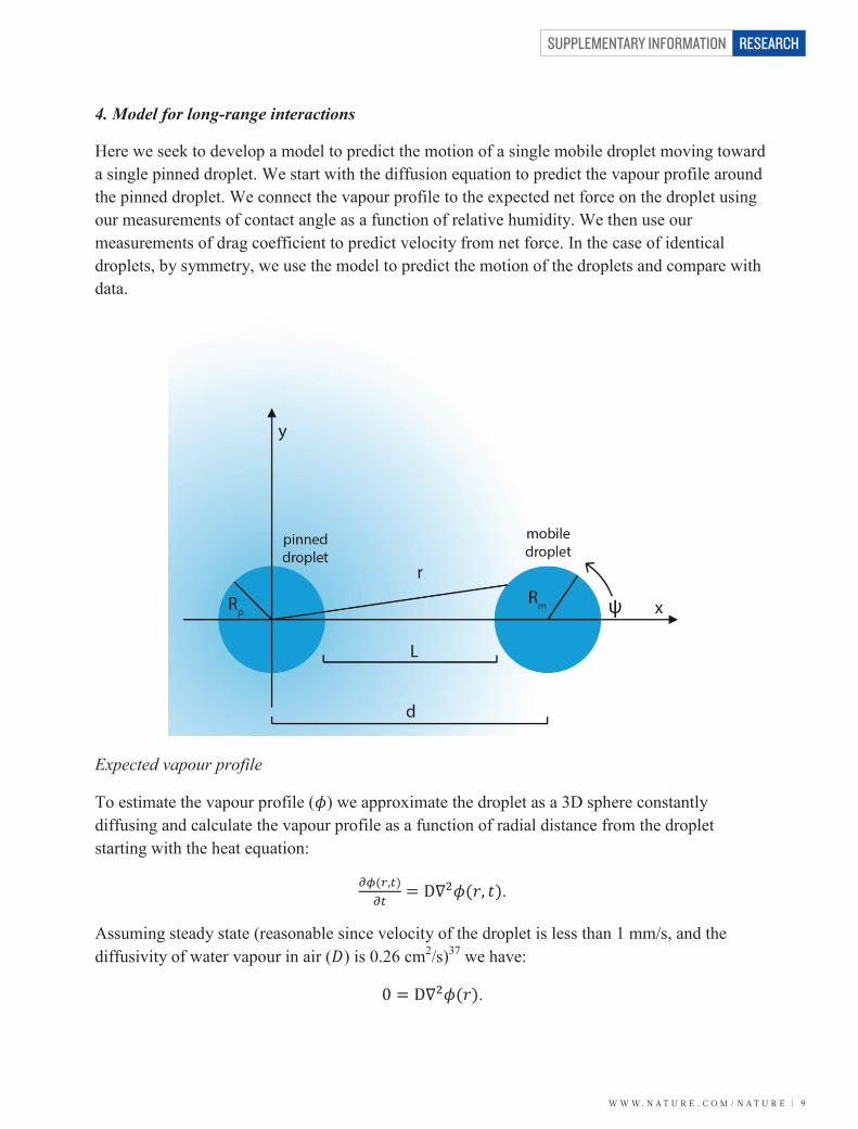
4. Model for long-range interactions
Here we seek to develop a model to predict the motion of a single mobile droplet moving toward a single pinned droplet. We start with the diffusion equation to predict the vapour profile around the pinned droplet. We connect the vapour profile to the expected net force on the droplet using our measurements of contact angle as a function of relative humidity. We then use our measurements of drag coefficient to predict velocity from net force. In the case of identical droplets, by symmetry, we use the model to predict the motion of the droplets and compare with data.
Expected vapour profile
To estimate the vapour profile (𝜙𝜙) we approximate the droplet as a 3D sphere constantly diffusing and calculate the vapour profile as a function of radial distance from the droplet starting with the heat equation:
𝜕𝜕𝜙𝜙(𝑟𝑟,𝑡𝑡)𝜕𝜕𝑡𝑡 = D∇2𝜙𝜙(𝑟𝑟, 𝑡𝑡).
Assuming steady state (reasonable since velocity of the droplet is less than 1 mm/s, and the diffusivity of water vapour in air (𝐷𝐷) is 0.26 cm2/s)37 we have:
0 = D∇2𝜙𝜙(𝑟𝑟).
SUPPLEMENTARY INFORMATION
1 0 | w w w. n a t u r e . c o m / n a t u r e
RESEARCH
11
Solving by assuming spherical symmetry around the droplet we obtain:
𝜙𝜙(𝑟𝑟) = 𝐶𝐶1r + 𝐶𝐶2.
Applying boundary conditions:
At infinity the vapour pressure is the relative humidity in the room (𝑅𝑅𝑅𝑅room) (𝑅𝑅𝑅𝑅 as a percentage of saturation):
𝜙𝜙(∞) = 𝑅𝑅𝑅𝑅room.
At the surface of the pinned droplet (𝑅𝑅𝑝𝑝) the concentration is dictated by the vapour pressure of water. Here we assume complete saturation since the droplets we are modelling here are primarily water (10% PG by volume and 2.6% PG by mole fraction). Raoult’s law can be used for a more accurate vapour pressure at extremely high PG concentrations. We obtain: 𝜙𝜙(𝑅𝑅p) =1. So:
𝜙𝜙(𝑟𝑟) = (1−𝑅𝑅𝑅𝑅room)𝑅𝑅pr + 𝑅𝑅𝑅𝑅room.
This approximation agrees well with analytical work on evaporating droplets that considers the complete spherical cap shape of the droplet on a solid substrate37.
Expected net force
Here we connect the vapour profile of the pinned droplet to the expected net force on the mobile droplet using measurements of contact angle on equilibrium droplets.
Considering a droplet at equilibrium, a force balance in the 𝑥𝑥 direction on the apparent contact line yields:
∑ 𝐹𝐹x = 0 = 𝛾𝛾LVfilm − 𝛾𝛾LVdropletcos (𝜃𝜃app).
So, knowing 𝛾𝛾LVdroplet, assuming it is independent of relative humidity, and measuring 𝜃𝜃app while varying relative humidity we can obtain 𝛾𝛾LVfilm(𝜙𝜙):
𝛾𝛾LVfilm(𝜙𝜙) = 𝛾𝛾LVdropletcos (𝜃𝜃app(𝜙𝜙)).
From measurements of contact angle on equilibrium droplets (10% PG) at various relative humidity, we know that cos(𝜃𝜃app) varies linearly with relative humidity (Fig. 2b):
cos(𝜃𝜃app(𝜙𝜙)) = 𝑚𝑚𝜙𝜙 + 𝑏𝑏
so substituting,
w w w. n a t u r e . c o m / n a t u r e | 1 1
SUPPLEMENTARY INFORMATION RESEARCH
12
𝛾𝛾LVfilm(𝜙𝜙) = 𝛾𝛾LVdroplet ∗ (𝑚𝑚𝜙𝜙 + 𝑏𝑏).
For a droplet experiencing a net force, assuming 𝜃𝜃app is constant (the Laplace pressure rapidly equilibrates droplets into a symmetrical spherical cap), the local force normal to the apparent contact line in the horizontal plane on the droplet (𝐹𝐹norm) is given by:
𝐹𝐹norm = 𝛾𝛾LVfilm(𝜙𝜙) − 𝛾𝛾LVdropletcos (𝜃𝜃app)
or, substituting the local film tension as a function of local relative humidity imposed by the other droplet:
𝐹𝐹norm = 𝛾𝛾LVdroplet(mϕ + b − cos(𝜃𝜃app)).
For an infinitesimal portion of the contact line, at known relative humidity and contact angle, the net force in the 𝑥𝑥 direction is given by:
𝑑𝑑𝐹𝐹net = 𝛾𝛾LVdroplet(mϕ + b − cos(𝜃𝜃app))cos (𝜓𝜓)𝑅𝑅m𝑑𝑑𝜓𝜓,
where 𝜓𝜓 is the parameterization of the droplet edge.
The total net force on the entire droplet is obtained by integrating 𝑑𝑑𝐹𝐹net around the droplet. This is given by the path integral:
Since 𝑑𝑑 and 𝑅𝑅m are of the same order, we are not able to further simplify this expression. We numerically integrate over time and obtain a plot of the position vs. time. Notice that in the text we discuss the case where 𝑅𝑅p = 𝑅𝑅m and both droplets are mobile. The mirror symmetry of this case (both droplets are identical and mobile) allows us to multiply the rate of variation of the distance between the droplets by two to account for the fact that both droplets are in motion. The model matches well with the observed data (Fig. 3b).
All parameters have been measured and none are fit. 𝐶𝐶drag is taken from our measurements of drag detailed in the ‘Measurement of drag’ section (𝐶𝐶drag = 1.94 mm
s∗μN ), m is taken from our
measurements of contact angle as a function of relative humidity (m = 0.025), 𝑅𝑅𝑅𝑅room is the measured humidity in the room at the time of the experiment (45%), 𝑅𝑅p = 𝑅𝑅m is the radius of the droplets as calculated in the ‘Comparison of experimental drag coefficient with theory’ section (1.39 mm), and 𝛾𝛾LVdroplet is taken from literature as described above in the ‘Surface tension of two-component mixtures’ section (61.5 mN/m for a 10% PG droplet).
w w w. n a t u r e . c o m / n a t u r e | 1 3
SUPPLEMENTARY INFORMATION RESEARCH
14
5. Assessment of thermocapillarity
Reverse flow (flow from edge to center of a droplet at the air interface) has been observed as a result of thermocapillary effects38. Here we investigate whether this effect could play a role in stabilizing our droplet system. Here we show that thermocapillarity does not appear to play a role in droplet stabilization in our system.
Very elegant theoretical and experimental work has shown that the ratio (kR = ks/kl) of conductivities between the solid substrate (ks) and liquid droplet (kl) is important for determining the effect of thermocapillarity39. For typical contact angles we observe any kR > ~1.8 should result in flow from the edge to the center of a droplet at the air interface (which might support droplet formation) and any kR < 1.8 should result in flow in the opposite direction (from center to edge of the dropletat the air interface) which might enhance droplet spreading (Extended Data Fig. 2). Others have shown that substrate thickness also plays a role; thin substrates are less effective at driving flow from edge to center40.
First, we note that thermocapillarity predicts flow from edge to center at the air interface for each liquid combination and pure liquid we tested (kR is always >1.8, except for pure water on the glass substrate used). If thermocapillarity were the dominant effect in droplet stabilization then each liquid pair and all individual liquids we tested should form droplets. However we observe that most of these pairs and all individual components do not form droplets, but instead spread (Fig. 2c, Extended Data Table 1). Our observations are well predicted by the rule we present which considers vapour pressure and surface tension. Furthermore, thermocapillarity arguments for stabilization only predict a monotonic change in contact angle with increasing PG concentration. Taken together these first observations show that thermocapillarity is not the driving mechanism for stabilizing these droplets.
We next sought to determine if we could detect any effects of thermocapillarity in droplet stabilization. We measured contact angles of PG/Water droplets on substrates with different thermal conductivities. We used a borosilicate glass slide for a conductive substrate (upon which thermocapillarity predicts flow from edge to center at the air interface), and plasma treated indium tin oxide coated polyethylene terephthalate (ITO/PET) as a low conductivity substrate (upon which thermocapillarity predicts flow center to edge at the air interface, assuming the 100 nm layer of ITO does not change the thermal conductivity of the bulk PET, a value of 0.19 W/(m*K)41), we also included a 136 μm coverslip, since substrate thickness has been shown to have an effect on reverse flow40. If thermocapillarity played a detectable role in droplet stabilization, we would expect to measure lower contact angles on the ITO/PET and coverslip. We did not detect any change in contact angles over the full range of PG concentrations, suggesting thermocapillarity plays no detectable role in droplet stabilization (Extended Data Fig. 3). Furthermore we noticed no change in direction of flow within droplets (as visualized by tracer beads), and no qualitative change in maximum flow velocity.
SUPPLEMENTARY INFORMATION
1 4 | w w w. n a t u r e . c o m / n a t u r e
RESEARCH
15
To understand why thermocapillarity does not appear to contribute, we referred to our model. The model requires a surface tension difference of 0.615-2.46 mN/m between the droplet and the film to support the contact angles we observe (depending on humidity as in Fig. 2b). Theoretical work predicts a temperature difference of up to 1 ºC for evaporating droplets on unheated substrates with thermocapillary induced flows42. This temperature difference results in an upper bound on the surface tension difference one could expect of 0.165 mN/m for the 10% PG droplets we used43. This is smaller than the smallest surface tension difference needed to support the droplets but at first glance might appear large enough to make a contribution to stabilization, however this temperature/surface tension gradient is spread over the entire radius of the droplet, while supporting a sharp contact angle would require an abrupt change at the contact line. Thermocapillarity does not provide such an abrupt jump in temperature/surface tension at the contact line, and hence doesn’t contribute strongly to stabilizing droplets. As a result of these observations and arguments listed, we neglect any contribution of thermocapillarity in our theory for predicting contact angle of these droplets.
w w w. n a t u r e . c o m / n a t u r e | 1 5
SUPPLEMENTARY INFORMATION RESEARCH
16
3. Supplementary videos:
Supplementary video 1. Long-range and short-range interactions in two-component droplets. Part 1) Complex movement of droplets. Highly dynamic behaviour of PG/water droplets of various concentrations and sizes when placed simultaneously on a corona treated glass slide. (Slide dimensions: 25 x 75 mm, 4x speed). Part 2) Long-range attraction, different concentrations. Two 0.5 µL droplets of 25% PG (blue) and 1% PG (orange) are placed near each other on a corona treated glass slide. First the droplets move toward each other, then the droplet of higher PG concentration ‘chases’ the droplet of lower PG concentration which ‘flees’. (1x speed). Part 3) Long-range attraction, same concentration. Two 0.5 µL droplets of 10% PG are placed near each other on a corona treated glass slide. Both droplets move toward each other, and then they merge. (1x speed).
Supplementary video 2. Internal flow. The first clip shows flow in a droplet on clean corona treated glass as visualized in bright field by 5 µm diameter tracer beads. The beads are initially well distributed but collect into a ring at the liquid/vapour interface. Flow can be seen moving both toward the centre and toward the edge of the droplet. The second clip shows a fluorescent movie of 2 µm diameter tracer beads visualizing flow in a droplet on high energy treated glass. Like this first clip, beads move both toward the centre and the edge of the droplet, collecting in a ring at the liquid/vapour interface. The third clip shows the same droplet as in the second clip, but on an untreated, unclean glass slide (lower energy surface). The bead velocity is much slower and beads do not collect into a ring. The droplets are 10% PG. (All clips are 2x speed).
Supplementary video 3. Long-range attraction. Part 1) Attraction across a break. Two 10% PG droplets moving toward each other despite a break/gap in the substrate. (1x speed). Part 2) Pipette tip control. A droplet of 10% PG moves to follow a pipette tip which contains a droplet of water. (Slide dimensions: 25 x 75 mm, 4x speed).
Supplementary video 4. Short-range chasing fluid exchange. Transfer of fluorescein arises from the back droplet (25 % PG, dyed with fluorescein) to the front droplet (1% PG, initially no fluorescein) during a short-range chasing interaction. The camera is panning to the right, following the droplet. (1x speed).
Supplementary video 5. Devices. Part 1) Self-alignment device. 25% PG droplets are placed in lanes and allowed to move. From initially random positions they spontaneously arrange themselves in a line. (Slide dimensions: 25 x 75 mm, 4x speed). Part 2) Circular chasing. A 25% PG droplet (blue) pursues a 1% PG droplet (red) around a 2.1 cm mean diameter circular ring several times before merging. (16x speed). Part 3) Vertical oscillator. A 1% PG droplet (red) is chased up by a 25% PG droplet (blue) which remains at the bottom of a vertical lane due to gravity. The 1% PG droplet is eventually overcome by gravity and falls back, only to oscillate again once it contacts the 25% PG droplet. (8x speed). Part 4) Movement on flexible substrates. Here we show short-range chasing on flexible strips of ITO/PET which have been
SUPPLEMENTARY INFORMATION
1 6 | w w w. n a t u r e . c o m / n a t u r e
RESEARCH
17
treated in a plasma oven for 5 min (droplets move on the high energy ITO side). Here a 25% PG droplet chases a 1% PG droplet in two different configurations. (4x speed).
Supplementary video 6. Self-sorting device. 0.25 µL droplets are deposited at the top of the device and gravity acts to bring them down. As they slide down the device, they sample each well. They are chased away if the surface tension of the well is lower than their own surface tension. They merge when they have reached the well of like surface tension (same [PG]). As in all videos and figures, the colour is only present to aid in visualization and not important in the phenomena. (4x speed).
Supplementary video 7. Repulsive long-range positioning. Here we demonstrate contactless remote droplet positioning. The top plate has droplets of pure PG, which act to repel the 10% PG red droplet via vapour through long-range repulsion interactions. When we arrange these PG droplets in a circle, they form a vapour trap which we move around to demonstrate positioning. (8x speed).
Supplementary video 8. Parallel plate devices. Part 1) Parallel plate alignment. Two 0.5 μL 10% PG droplets (blue on top, yellow on the bottom) interact across an air gap via their vapour clouds on the adjacent side of two parallel glass slides. Here the slides are repositioned several times to show several examples of alignment. (8x speed). Part 2) Self-assembled, self-aligned 2-lens system. Here we use a similar configuration to the parallel plate aligner but use clear droplets and arrange the distance between the plates to create an image only once alignment has occurred. This system shows how lenses can be placed far apart and will self-assemble and self-align to produce images of various magnifications, depending on distances and curvatures of the lenses. (2x speed, and 4x speed). Part 3) Self-assembled, self-aligned 3-lens system with scanning. Here we show an optical system where 3 lenses with 4 optical surfaces self-assemble and self-align. The setup is similar to the 2-lens system with an additional plate inserted between the top and bottom plates. This additional plate has a hole drilled through it in which sits a pinned droplet with two optical surfaces. We then demonstrate the ability of this system to scan an area much larger than the lens itself by moving the center plate. When the center plate is moved, the other lenses follow then automatically realign (2x speed, and 8x speed).
Supplementary video 9. Easy way to recreate. Here we demonstrate an easy method to create the simplest version of this system and run basic experiments. For more detailed methods please refer to the methods section (Supplementary Information Section 1). (various speeds).
w w w. n a t u r e . c o m / n a t u r e | 1 7
SUPPLEMENTARY INFORMATION RESEARCH
18
4. Supplementary references:
33 Allain, C., Ausserre, D. & Rondelez, F. A New Method for Contact-Angle Measurements of Sessile Drops. J Colloid Interf Sci 107, 5-13, (1985).
34 Brochard, F. Motions of Droplets on Solid-Surfaces Induced by Chemical or Thermal-Gradients. Langmuir 5, 432-438, (1989).
35 George, J. & Sastry, N. V. Densities, dynamic viscosities, speeds of sound, and relative permittivities for water plus alkanediols (propane-1,2- and -1,3-diol and butane-1,2-,-1,3-,-1,4-, and -2,3-diol) at different temperatures. J Chem Eng Data 48, 1529-1539, (2003).
36 Karpitschka, S. & Riegler, H. Quantitative Experimental Study on the Transition between Fast and Delayed Coalescence of Sessile Droplets with Different but Completely Miscible Liquids. Langmuir 26, 11823-11829, (2010).
37 Hu, H. & Larson, R. G. Evaporation of a sessile droplet on a substrate. J Phys Chem B 106, 1334-1344, (2002).
38 Hu, H. & Larson, R. G. Analysis of the effects of Marangoni stresses on the microflow in an evaporating sessile droplet. Langmuir 21, 3972-3980, (2005).
39 Ristenpart, W. D., Kim, P. G., Domingues, C., Wan, J. & Stone, H. A. Influence of substrate conductivity on circulation reversal in evaporating drops. Phys Rev Lett 99, (2007).
40 Xu, X. F., Luo, J. B. & Guo, D. Criterion for Reversal of Thermal Marangoni Flow in Drying Drops. Langmuir 26, 1918-1922, (2010).
41 Lopes, C. & Felisberti, M. I. Thermal conductivity of PET/(LDPE/AI) composites determined by MDSC. Polymer testing 23, 637-643 (2004).
42 Bhardwaj, R., Fang, X. H. & Attinger, D. Pattern formation during the evaporation of a colloidal nanoliter drop: a numerical and experimental study. New J Phys 11, (2009).
43 Khattab, I. S., Bandarkar, F., Khoubnasabjafari, M. & Jouyban, A. Density, viscosity, surface tension, and molar volume of propylene glycol+water mixtures from 293 to 323K and correlations by the Jouyban–Acree model. Arabian Journal of Chemistry (2012).