SUPPLEMENTARY INFORMATION - Nature · The glacier bedrock consists of Precambrian to Paleozoic...

1. Sedimentary basin characteristics

A summary of the inferred characteristics of Antarctic sedimentary basins (ASBs) is presented in

Suppl. Table 1, compiled from published geophysical datasets. Geophysical datasets indicate that

these basins penetrate several 100km-1000km into the Antarctic interior1-4, and are associated

with the onset of accelerated ice motion in ice streams and their tributaries5. The inferred origin

of these sediments is marine4,6, glaci-marine and crustal sedimentary sources1. The widespread

presence of dissolved methane, together with geochemical evidence for methanogenesis in

marine cores, rock cores and seeps around the Antarctic margin indicates that OC is commonly

cycled to methane in ocean margin basins7-12. We would expect similar processes to prevail in

sedimentary basins beneath the ice sheet.

Based upon BEDMAP data and previous interpretations of this dataset4, we calculated the areas

of the West (WAIS) and East Antarctic Ice Sheets (EAIS) underlain by sedimentary basins. We

assume that the seaward extent of these basins is the present day grounding line and that the

WAIS and EAIS were present at similar extents to the present day for 1 and ~30 Ma13-15

respectively, where the 1 Ma value is maximum estimate indicated by recent modelling14. This

gave aerial extents of 50% ice sheet area (or 1 x 106 km2) for WAIS and 25% area (or 2.5 x 106

km2) for EAIS. Combining a map of the thermal conditions at the base of the ice sheet (cold

versus warm)16 with the BEDMAP data for ASB extent indicates that approximately 20% of

EAIS (e.g. parts of the Aurora Subglacial Basin4) and 10% of WAIS basins are in cold bed zones

and likely to exhibit frozen conditions at the sediment surface. The latter are used to calculate

methane hydrate accumulation under our “Zero Flux” scenario. The remaining wet-based area of

WWW.NATURE.COM/NATURE | 1

SUPPLEMENTARY INFORMATIONdoi:10.1038/nature11374

the ASBs is used to calculate the hydrate inventory for the “Maximum Flux” scenario. Further

details of these scenarios can be found in Supplementary Information 2f, iii.

Supplementary Table 1 – Summary of characteristics of sedimentary basins in East and

West Antarctica as inferred from geophysical surveys

Sedimentary Basin Location Sediment depth Ice thickness Reference East Antarctic Ice Sheet Wilkes Land Subglacial Basin 1.5-3km 3km 1

Adventure Subglacial Trench 5-10km 3.5km 17,18

Coats Land, Slessor Glacier (Filchner Ice Shelf) 3 km 2-2.8km 19,20

Prydz Bay Basin, Lambert Glacier several km <2.5km 21 22

South Pole 0.2km 2.8km 3

Vostok Basin 10km 3.6km 2

Aurora Basin 1km 3km 23

West Antarctic Ice Sheet Ross Sea Subglacial Basins Victoria Land Basin/Terror Rift 5-14km 2km 24-27

Central Trough 7-8km 2km 27-29

Eastern Basin (WAIS fed) i. Whillans Ice Stream (B)

0.6km

1km

30,31

i. Kamb Ice Stream (C) 0.2-2km 1km 32,33

i. Ice Stream D 0.1-1km 1km 32,34

v. Siple Dome 0.3km 1km 3

Rutford Ice Stream (Ronne-Filchner) 0.6-1km 2-3km 6

Mary Byrd Land Mary Byrd Land Dome Bentley Subglacial Trench

0.26km 0.55km

1.9km 3.2km

3,35

3,35


SUPPLEMENTARY INFORMATIONRESEARCHdoi:10.1038/nature11374

2. Supplementary Methods

a. Field sampling

Subglacial sediment and debris-rich basal ice were collected from Lower Wright Glacier,

(Antarctica) Russell Glacier (Greenland) and John Evans Glacier (Canadian Arctic) from

marginal locations. Basal ice samples from all three sites included organic matter overridden

during the late Holocene. This carbon derived from lake sediments in the Antarctic and Canadian

Arctic cases, indicated by the presence of chlorophyll-containing algal cells, and from overridden

paleosols in Greenland36. Details of the sites are as follows:

Lower Wright Glacier drains from the Wilson Piedmont Glacier in the McMurdo Dry Valleys

region of Antarctica, and currently terminates in the permanently ice-covered Lake Brownworth.

The glacier bedrock consists of Precambrian to Paleozoic metasediments, granite-gneisses and

lamprophyre and rhyolite porphyry dikes, as well as Jurassic-age dolerite sills37. In the past 2-3

centuries the glacier advanced and reworked lake sediments into low moraines consisting of fine-

grained sand, silt and lacustrine algae. Large blocks of frozen sediments intercalated with layers

of pure glacier ice and basal ice are exposed at the terminus. The sampling was conducted from

ice exposed at the crest of the moraine along the interface between the glacier and the perennially

ice-covered Lake Brownworth. Three separate blocks were cut with a chain saw across a

sequence in which an ice layer 21 cm thick was sandwiched between two layers of frozen mud,

with algal mats along the ice mud contacts.

Russell Glacier is an outlet glacier of the western margin of the Greenland Ice Sheet. The

bedrock consists of Archaean gneiss reworked in the early Proterozoic38. Analyses based on 14C



dated moraines suggest a highly dynamic regional ice margin with many Holocene re-advances,

including two significant re-advances between 4.8–4.4 ka BP and 2.5–2 ka BP over quaternary

deposits containing fresh organic matter. From ~700 a BP to the present, the ice margin has

undergone minor retreats and re-advances39. Samples were collected from the glacier terminus,

where subglacial material is exposed at the ice-margins. The outermost surface of ice (up to 1 m)

was removed by chain sawing in order to expose ice that was not subject to modern

contamination. Then, large cube-shaped samples (~35×35×35 cm) were chain sawed from the

ice, containing subglacial sediment, debris-rich basal ice and clean glacial ice.

John Evan’s Glacier is a large valley glacier located at 79°40N, 74°00W, on the east coast of

Ellesmere Island, Nunavut, Canada. It covers approximately 75% of a 220-km2 catchment, with

a length of 15 km and an elevation range of 100 to 1500 m above sea level. The glacier is

polythermal, with cold-based ice in the accumulation area and at the glacier margins where ice is

thin and warm-based ice throughout the remainder of the ablation zone, where basal water is

present. The glacier is underlain by an Ordovician/Silurian carbonate/evaporite sequence with a

minor clastic component. Shale containing small amounts of pyrite outcrops are present near the

glacier terminus. Sampling was conducted in July 2002 from an exposure of basal ice in a

crevasse wall at the southern margin of the glacier, using the protocols described in 40. Samples

were kept in sealed sterile Whirlpak bags and transported frozen to University of Alberta and

stored at -20°C until transport (frozen) to Bristol in summer 2008. The sample analysed

consisted of clear basal ice containing layers and lenses of fine- grained mud with obvious

organic content, and some coarser material. This material was probably deposited in an ice-

marginal pond and accreted onto the base of the glacier during a period of advance.



All the collected samples of debris-rich basal ice and subglacial sediment were transported

frozen to the Low Temperature Experimental Facility (LOWTEX) at Bristol and stored at -30°C.

Prior to analysis and/or incubation experiments, the samples were placed in a laminar flow

cabinet to prevent contamination and the outer layer (10-30 mm) of each sample was removed by

washing with deionised water. The ice samples were then placed in a pre-furnaced glass bowl

and allowed to thaw. The liberated sediment and the melted ice were used for further analysis.

Ice samples with sediment to be used for incubation experiments (see 1b) were thawed in an

anaerobic chamber under a 5%H2, 10%CO2, 85% N2 atmosphere.

b. Incubation Experiments on subglacial overridden material

Two grams of wet subglacial sediment with 8 ml of glacial meltwater from Lower Wright

Glacier, Russell Glacier and John Evans Glacier was incubated in pre-furnaced 12 ml glass

serum vials sealed with Bellco butyl rubber stoppers (Bellco Glass, Vineland, NJ), resulting in

2.5 ml of headspace in each vial. Controls were prepared by furnacing the sediment at 140°C for

5 h prior to incubation and using autoclaved deionised water instead of meltwater. Three

parallels for each sample were incubated at 1, 4 and 10°C in the dark for up to 720 days. Initial

microcosm preparation (defrosting sediment, weighing into vials, adding water and stoppering)

was performed in an anaerobic chamber under a 5%H2, 10%CO2, 85% N2 atmosphere. Vials

were then removed from the chamber and flushed for 10 minutes with a mixture of N2 with 380

ppm CO2. They were then overpressurised to 1.5 atm with the N2/380 ppm CO2 mix. CH4 in the

headspace was analysed on a Varian 3800 gas chromatograph (Varian, Palo Alto, CA), using a

2m × 1/8 inch Hayesep-Q column, 80-100 mesh size. An isothermal temperature of 50°C was

used throughout the runs. The detection limit was 1.6 ppmv. Samples from all temperatures were



transferred to a cold bath (1°C) prior to measurement. The CH4 concentrations in the headspace

of samples from 4 and 10°C were then temperature-corrected and all concentrations were

corrected for dissolved CH4 41. The CH4 ppmv values were then converted into moles using the

ideal gas law (Suppl. Equation 1).

n = pV/RT × 0.000001 × [CH4]ppmv (Suppl. Eq. 1)

where n is the amount of CH4 in mol, p is the pressure (1.5 atm), V is the headspace volume

(0.0025 l), R is the gas constant (~0.0821 l atm K-1 mol-1), T is the temperature (274.15 K =

1°C), and [CH4]ppmv the concentration of CH4 in ppmv.

c. Elemental Analysis on subglacial sediments

The total carbon (TC) concentration in the basal ice and subglacial sediment samples was

determined using a EuroVector EA3000 Elemental Analyser (EuroVector, Milan, Italy). The

concentration of inorganic carbon (IC) was measured on a Strohlein Coulomat 702 analyser

(Strohlein Instruments, Kaarst, Germany) adapted for this purpose. Both analysers were

calibrated using certified standards. The detection limit was 10 ppm for both analyses, and the

precision of determinations was 0.3%. The total organic carbon (TOC) concentration in the

samples was calculated as the difference between TC and IC.

d. Calculation of rates of methanogenesis from experimental data

Rates of methane production (Rxn, in fmol C as CH4 g-1 hr-1) are calculated from experimental

data according to Suppl. Equation 2.



(Suppl. Eq. 2)

Where and are the mean amounts of methane (in fmol) measured in

experimental vials minus the amount of methane measured in killed controls (in fmol, where

mean values derive from triplicates) at the start (t=0) and at the end of the incubations (t=final)

respectively. Md is the dry mass of subglacial sediment used in incubations and T is the total

incubation time in hours.

e. Calculation of the duration of anaerobic methane oxidation (AOM) in the marine

sediment/till complex

We assume that methane oxidation largely occurs anerobically, coupled to sulphate reduction.

This is consistent with data that suggests that subglacial till is anoxic42,43. We calculate the

maximum possible duration of AOM in the marine sediment/till complex in Antarctic marine

sedimentary basins in the following manner. We assume that AOM occurs in a similar manner to

sub-sea floor sediments, where it is coupled to sulphate reduction44 (Suppl. Equation 3). Hence,

the ultimate control on the amount of methane that can be oxidized is the size of the sulphate

pool.

(Suppl. Eq. 3)

Sulphate in the subglacial marine sediment/till complex derives from two sources which are

finite. First, sulphate is generated via the oxidation of sulphides present in the subglacial till.



Assuming a mean sulphide content for bedrock of 0.3%45, a mean rock density of 2650 kg m3

and a porosity for subglacial till of 0.446, there is approximately 15.9 kg (=133 moles) sulphide

(FeS2) present in a 5 m x 1 m2 till layer. This gives 265 moles of sulphate available for AOM

(Suppl. Equation 4) within the same sediment volume.

(Suppl. Eq. 4)

Second, the overridden marine sediment contains a finite sulphate pool derived from seawater.

We calculate that the total sulphate pool is 630 mol based on typical Antarctic marine porewater

sulphate profiles10, where the sulphate reduction zone extends to 150 m below the sea floor. As

in sub-sea floor sediments, we would expect a proportion of this sulphate to be consumed by

sulphate reduction that is not coupled of AOM.

Having calculated the size of the marine sediment/till complex sediment sulphate pool, we

calculate the total amount of time over which AOM could occur (coupled to sulphate reduction),

using rates of AOM reported in the marine literature. AOM in sub-sea floor sediments occurs

within the sulphate reduction zone at rates that vary by several orders of magnitude47,48

depending on factors affecting rates of microbiological activity, including the upward methane

flux49. Hence, in diffusion-dominated sediments such as those described in this paper, AOM

rates may be expected to be orders of magnitude lower than those in high CH4 environments50.

We calculate the total amount of time (T) required for AOM to exhaust the seawater- and till-

derived sulphate in Antarctic sedimentary basins (T) according to Suppl. Eq. 5:



(Suppl. Eq. 5)

where SO42—till and SO4

2—marine are the total sulphate pools present in the subglacial till and

overridden marine sediments respectively (in mol), RAOM is the rate of AOM in mol m-3 a-1 and

V is the volume of the sediment column in which AOM is active (assumed to be 150 m in this

case). We employ a minimum rate for AOM (0.001 ng cm-3 d-1 or ~25 fmol g-1 hr-1), which

scales well to our most realistic, modelled rates of methane production in surface sediments (10

fmol g-1 hr-1; see Section g) and aligns with minimum values reported in the literature for marine

hydrate areas via modelling48. By using minimum rates for AOM, we generate a maximum

possible duration for AOM and hence, a minimum value for methane accumulation in sediments.

This gives a total of 16 ka for the amount of time (T) needed for AOM to exhaust the sulphate

pool. This duration is short relative to the duration of glaciations in Antarctica (Ma).

f. Numerical modelling of methane production in Antarctic Sedimentary basins

We employ a well-established 1d numerical hydrate model51, originally developed to model

methane hydrate accumulation beneath the sea floor. We assume physical properties for

sediments similar to those previously employed for ocean sediment modelling, and listed in 51.

Site specific parameters are given in Suppl. Table 2. The justification for the parameterisations

which are specific to subglacial sediments are provided in the following text.



Supplementary Table 2 Site specific parameters employed in hydrate modelling

Symbol Parameter Value Units h Ice thickness 1000 (WAIS), 2000

(EAIS) m

D Depth of hydrate stability zone 282 (WAIS), 663 (EAIS)

m

2D Depth of conceptual domain 564 (WAIS), 1326 (EAIS)

m

G Geothermal gradient 0.05 (WAIS), 0.03 (EAIS),

°C m-1

φ0 Sediment porosity at the sediment surface

0.58 -

Z0 e-folding depth of porosity 2200 m S Sedimentation rate 0 M a-1

T(0) Sediment surface temperature 0 TOC(0,0) Total organic carbon at sediment

surface 0.2-5 %

α(0) Available organic carbon at sediment surface

1.0 -

k Rate constant for methanogenesis Variable (SF2) - Rxn Rate of methanogenesis Variable (SF2) fmol C as CH4 g-1

(dry sediment) hr-1

The model computes the methane mass of hydrate in units of kg m-2. It sums up the product of

cell porosity and the fraction of porespare occupied by hydrate for the entire column. This value

is then multiplied by the density of methane hydrate (930 kg m-3)52, the cell thickness (in m), and

the fractional contribution of methane to the mass of the hydrate complex [i.e. 1 mole of

methane hydrate has a mass of 119.65 g, the fractional contribution of methane to the mass is

16.04/119.65=0.134 assuming complete cage occupancy]. The results are produced in mass CH4,

hence Kg CH4 m-2, and one can convert the areal density of methane to units of carbon by

multiplying by 0.75. We also state total hydrate+gas inventories in the main manuscript in units

of volume (m3), assuming that 1 mole of methane gas equates to 0.0224 m3 at standard



temperature and pressure.

i. Fluid Flow. Our assumption of zero fluid flow for simulations focussed on

biogenic methane production (rather than thermogenic) is justified by there being zero

sedimentation beneath the ice sheet, which would normally drive sediment compaction, and very

low methane production rates. These two factors normally drive fluid flow in a typical marine

sediment53. This gives us a conservative treatment of methane accumulation in this case, since

fluid flow tends to enhance methane hydrate accumulation by enabling its transportation to the

hydrate stability zone53. Model simulations that are conducted to test the sensitivity of methane

hydrate inventories to thermogenic methane production beneath WAIS do employ fluid flow,

over a spectrum of velocities found in the literature (see main article). We assume methane

concentrations in the upward advecting fluid of 100% saturation.

ii. Glacial erosion. We appreciate that glacial erosion may lead to some sediment

removal or re-distribution over time. Indeed, where ice is warm at the bed and exhibiting high

rates of flow (e.g. close to the ice sheet margins), erosion rates could be considerable. For

example, 54 estimate maximum erosion rates of 0.6mm a-1 in ice stream tributaries, but this

upstream effect is partially negated by deposition downstream in ice stream trunks. More recent

work indicates that such high erosion rates are incompatible with the preservation of sedimentary

basins beneath the ice sheet and that lower erosion rates must be present over a large proportion

of these basins in order for sediments to still be present up to 30 Ma of glaciation19. Erosion rates

of 0.04 mm a-1 have been calculated for Slessor Glacier in East Antarctica19, and rates as low as

0.001 mm a-1 for the Lambert basin (East Antarctica)55. For WAIS, these latter rates give 1-40m



of erosion over 1Ma, which is a small proportion of the total sediment thickness in the model

(1km). For East Antarctica, where basins contain several km of sediment (see Suppl. Table 1),

erosion could remove 30-1200m of sediment over 30 Ma. While we do not explicitly include

erosion in the model, we do account for some removal of material by assuming a relatively low

(~1km) sediment thickness (Suppl. Table 1).

iii. Porosity and basal temperatures. To obtain a vertical porosity profile that is

representative of Antarctic subglacial sedimentary basins, we fit an exponential curve56 to

porosity data from the >1km-deep ANDRILL borehole drilled into a largely marine sedimentary

sequence beneath the McMurdo Ice Shelf (MIS)57. Whereas this marginal sedimentary basin may

have undergone some more ice sheet retreat-advance cycles than inland subglacial basins, no

other deep Antarctic porosity profile is available. The linear least squares fit has the form (SF1

and 2):

)/exp( ozzo −= φφ (Suppl. Eq. 6)

with oφ as the fitted porosity (~0.58) at the top of the sedimentary column where z = 0 and zo as

the e-folding depth (~2200m). We obtained the best fit numerically by considering 10,000

different combinations of oφ and zo, and minimizing with respect to the Root Mean Square

Deviation. The best fit had a RMSD of 0.12. For comparison, the worst fit, we obtained had a

RMSD of 0.72.



Supplementary Figure 1 (SF1) Observed porosity profile from the ANDRILL borehole, with

the line of bet fit indicated (employed for the modelled porosity profile)

We consider two separate cases for temperature gradients in our calculation. Given that

geophysical estimates of geothermal flux consistently indicate lower heat flow for East

Antarctica than for West Antarctica58,59, we assume a moderate temperature gradient of 0.03

°C/m for the former and a steeper gradient of 0.05 °C/m for the latter. Using the average thermal

conductivity of the sedimentary sequence in the ANDRILL MIS borehole of ~1.5 mW/°C57,

these temperature gradients are equivalent to geothermal fluxes of 45 and 75 mW/m2

respectively.

In order to consider how temperature conditions at the ice sheet sole might influence methane

hydrate formation, we define two end member scenarios to take account of wet-based and cold-

based conditions. Under our Maximum Flux scenario, simulating warm-based conditions,

methane diffuses out of the sediment column according to the diffusion equation. Under our Zero



Flux Scenario, there is no methane diffusion out of the top of the sediment column. The latter

situation is representative of frozen basal conditions or conditions at the bed where basal melt

rates are very low and small fluxes of methane in a water layer at the ice-bed interface are

exceeded by methane diffusion out of the top of the sediment column. In the latter case,

concentration gradients of methane in the upper sediment column flatten over time and methane

diffusion might reduce to very low or zero values.

iv. Organic matter degradation sub-model

We consider that the first order control on rates of methanogenesis is organic matter quality,

rather than temperature60. This is consistent with work conducted elsewhere on marine

sediments60. Hence, methane production rates in the model (Rxn(z,t)) are scaled to decreasing

organic matter quality with sediment age, and hence depth, using a reactive continuum model61.

We prescribe an initial total organic carbon (TOC) depth profile of subglacial Antarctic marine

sediments (TOC(z,0)) that is calculated from the steady-state state solution of organic carbon

using the reactive continuum model (Suppl. Equation 7) and assuming a prescribed surface

organic carbon content TOC(0,0) (see Supplementary Methods 3a), as well as an age/depth

model age(z). The age/depth model is constructed using a cubic spline interpolation of observed

depth/age relationships in circum-Antarctic marine sediments7. This age depth model is

presented in SF2.

TOC(z,0) = TOC(0,0)⋅a

a + age(z)⎛

⎝ ⎜

⎞

⎠ ⎟

υ

(Suppl. Eq. 7)



Where, a is the average life-time of the most reactive components of the bulk organic matter, and

taken to be 5000 a in this case according to the relationship of “a” with sedimentation rates61,

where values for the latter are derived from our age/depth model. The parameter v (referred to as

the reactivity parameter in the main manuscript) determines the shape of the underlying gamma

distribution61. Sensitivity of total releasable methane accumulation to the v parameter and

TOC(0,0) is explored in a full model sensitivity analysis (Supplementary Methods 3) .

In a closed system (i.e. non-mixed sediment), the depth-profile of the organic matter reactivity

(k(z,0)) is calculated according to Suppl. Equation 8 61,62.

(Suppl. Eq 8)

Hence, the initial rate of methane production by unit volume dry sediment at any depth within

the sediment profile is calculated as follows:

(Suppl. Eq. 9)

Thus, the rate of methane production by methanogenesis by unit volume porewater is calculated

as follows:

(Suppl. Eq. 10)



Where, ρg is the density of sediment grains, ρf denotes the density of porewater and MCH4/MTOC

is the ratio between the molar mass of methane and carbon. We subsequently run the model

transiently for the duration of glaciation in Antarctica. In doing so, we account for the decrease

in TOC over time, (Suppl. Equation 11), generating new values for the TOC content

of sediments ( ) for each depth/time interval, dependent upon the aging of the material

(Suppl. Equation 12). These simulated TOC profiles and resulting rates of methanogenesis are

presented in SF2 for four different time steps (t=0, 1 Ma, 10Ma and 30Ma) for values of v=0.1

and v-0.01.

(Suppl. Eq. 11)

(Suppl. Eq. 12)

We use an additional modification of the methane production term, Rxn, in Suppl. Equation 9, to

take into account the consumption of methane that takes place via AOM coupled to sulphate

reduction in marine sedimentary sequences. This effect is parameterized in our model by setting

methane production to zero in the top 150m of the model domain for the first 16 ka of the

simulation time, by which time the sulphate reservoir trapped at the time of glaciation is assumed

to be exhausted (see Supplementary Methods 1e for explanation). During this 16 ka, the model

calculates the degradation of OM above the sulphate penetration depth (150m) by non-

methanogenic pathways. This TOC degradation does obviously not contribute to CH4 generation.



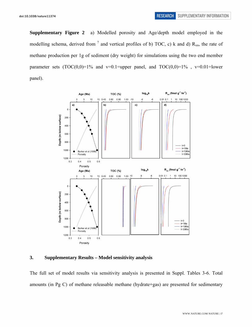
Supplementary Figure 2 a) Modelled porosity and Age/depth model employed in the

modelling schema, derived from 7 and vertical profiles of b) TOC, c) k and d) Rxn, the rate of

methane production per 1g of sediment (dry weight) for simulations using the two end member

parameter sets (TOC(0,0)=1% and v=0.1=upper panel, and TOC(0,0)=1% , v=0.01=lower

panel).

3. Supplementary Results – Model sensitivity analysis

The full set of model results via sensitivity analysis is presented in Suppl. Tables 3-6. Total

amounts (in Pg C) of methane releasable methane (hydrate+gas) are presented for sedimentary



basins beneath EAIS and WAIS under Zero Flux and Maximum Loss Scenarios, employing a

simulation time of 30 Ma for EAIS and 1 Ma for WAIS. The parameters v, OM and initial

methane saturation of sediment porewaters with respect to methane are varied in the sensitivity

analysis. As described in the main article, we assume areas of 1 x 106 and 2 x 106 km2 for WAIS

and EAIS respectively. These results will be referred to in the following sections.

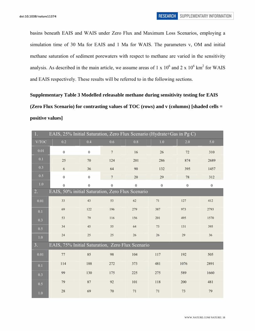
Supplementary Table 3 Modelled releasable methane during sensitivity testing for EAIS

(Zero Flux Scenario) for contrasting values of TOC (rows) and v (columns) [shaded cells =

positive values]

1. EAIS, 25% Initial Saturation, Zero Flux Scenario (Hydrate+Gas in Pg C) V/TOC 0.2 0.4 0.6 0.8 1.0 2.0 5.0

0.01 0 0 7 16 26 72 310

0.1 25 70 124 201 286 874 2689

0.3 6 36 64 90 132 395 1457

0.5 0 0 7 20 29 78 312

1.0 0 0 0 0 0 0 0

2. EAIS, 50% initial Saturation, Zero Flux Scenario

0.01 33 43 53 62 71 127 412

0.1 69 122 196 279 387 973 2793

0.3 53 79 116 156 201 495 1570

0.5 34 45 55 64 73 131 395

1.0 24 25 25 26 26 29 36

3. EAIS, 75% Initial Saturation, Zero Flux Scenario

0.01 77 85 98 104 117 192 505

0.1 114 188 272 373 481 1076 2891

0.3 99 130 175 225 275 589 1660

0.5 79 87 92 101 118 200 481

1.0 28 69 70 71 71 73 79



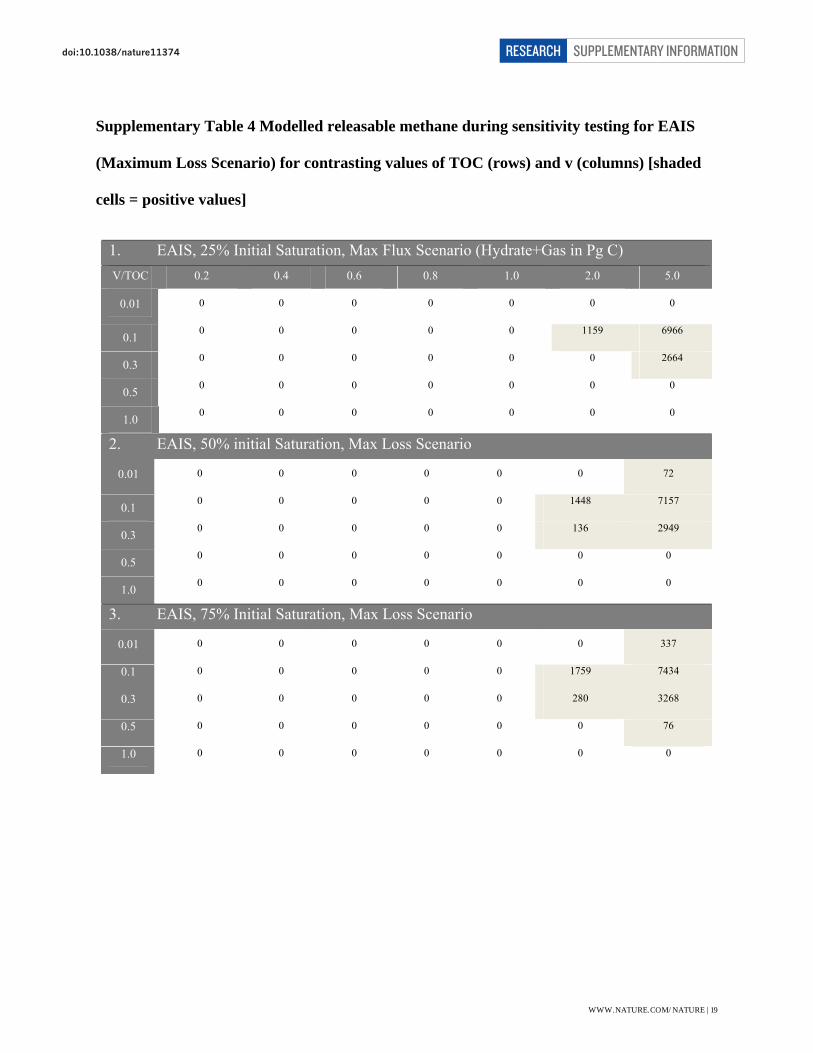
Supplementary Table 4 Modelled releasable methane during sensitivity testing for EAIS

(Maximum Loss Scenario) for contrasting values of TOC (rows) and v (columns) [shaded

cells = positive values]

1. EAIS, 25% Initial Saturation, Max Flux Scenario (Hydrate+Gas in Pg C) V/TOC 0.2 0.4 0.6 0.8 1.0 2.0 5.0

0.01 0 0 0 0 0 0 0

0.1 0 0 0 0 0 1159 6966

0.3 0 0 0 0 0 0 2664

0.5 0 0 0 0 0 0 0

1.0 0 0 0 0 0 0 0

2. EAIS, 50% initial Saturation, Max Loss Scenario

0.01 0 0 0 0 0 0 72

0.1 0 0 0 0 0 1448 7157

0.3 0 0 0 0 0 136 2949

0.5 0 0 0 0 0 0 0

1.0 0 0 0 0 0 0 0

3. EAIS, 75% Initial Saturation, Max Loss Scenario

0.01 0 0 0 0 0 0 337

0.1 0 0 0 0 0 1759 7434

0.3 0 0 0 0 0 280 3268

0.5 0 0 0 0 0 0 76

1.0 0 0 0 0 0 0 0



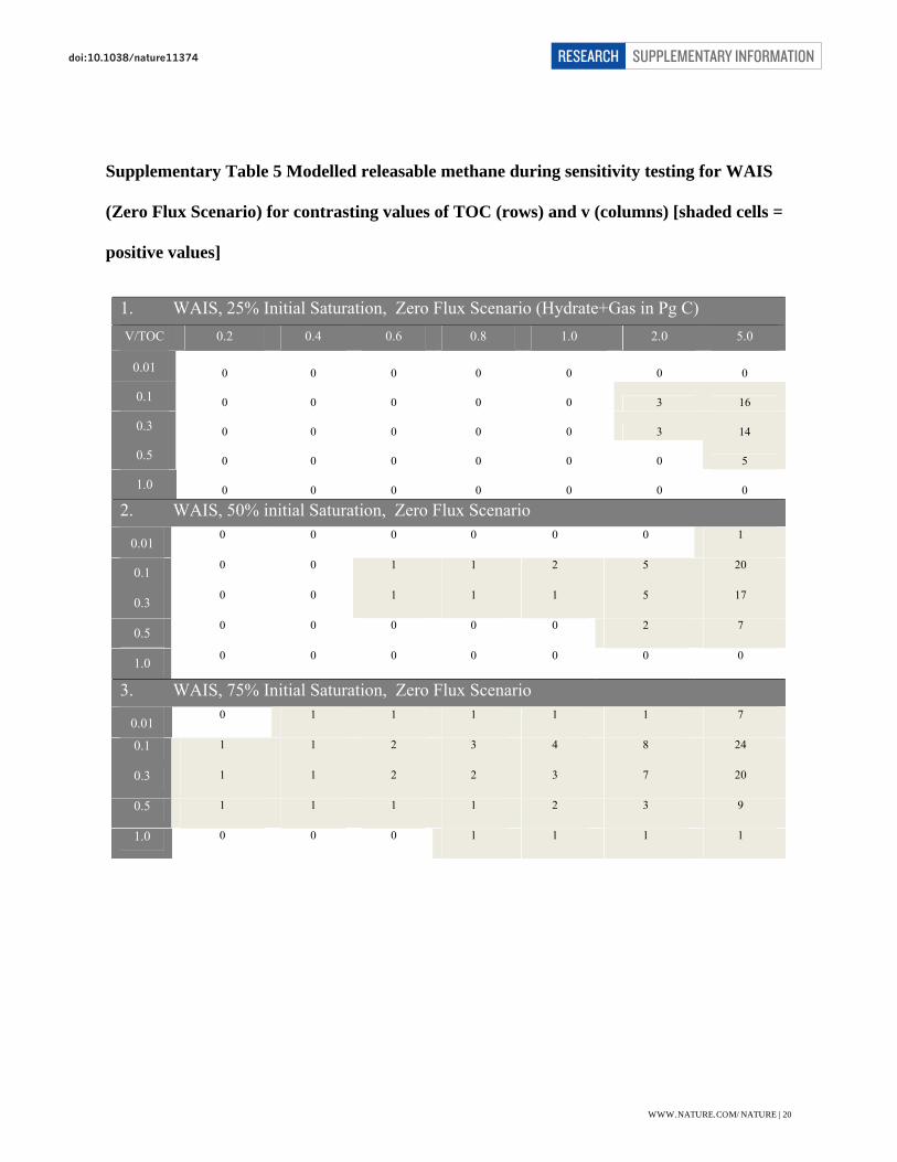
Supplementary Table 5 Modelled releasable methane during sensitivity testing for WAIS

(Zero Flux Scenario) for contrasting values of TOC (rows) and v (columns) [shaded cells =

positive values]

1. WAIS, 25% Initial Saturation, Zero Flux Scenario (Hydrate+Gas in Pg C) V/TOC 0.2 0.4 0.6 0.8 1.0 2.0 5.0

0.01 0 0 0 0 0 0 0

0.1 0 0 0 0 0 3 16

0.3 0 0 0 0 0 3 14

0.5 0 0 0 0 0 0 5

1.0 0 0 0 0 0 0 0

2. WAIS, 50% initial Saturation, Zero Flux Scenario

0.01 0 0 0 0 0 0 1

0.1 0 0 1 1 2 5 20

0.3 0 0 1 1 1 5 17

0.5 0 0 0 0 0 2 7

1.0 0 0 0 0 0 0 0

3. WAIS, 75% Initial Saturation, Zero Flux Scenario

0.01 0 1 1 1 1 1 7

0.1 1 1 2 3 4 8 24

0.3 1 1 2 2 3 7 20

0.5 1 1 1 1 2 3 9

1.0 0 0 0 1 1 1 1



Supplementary Table 6 Modelled releasable methane during sensitivity testing for WAIS

(Maximum Loss Scenario) for contrasting values of TOC (rows) and v (columns) [shaded

cells = positive values]

1. WAIS, 25% Initial Saturation, Maximum Flux Scenario (Hydrate+Gas in Pg C) V/TOC 0.2 0.4 0.6 0.8 1.0 2.0 5.0

0.01 0 0 0 0 0 0 0

0.1 0 0 0 0 0 0 17

0.3 0 0 0 0 0 0 0

0.5 0 0 0 0 0 0 0

1.0 0 0 0 0 0 0 0

2. WAIS, 50% initial Saturation, Maximum Flux Scenario

0.01 0 0 0 0 0 0 0

0.1 0 0 0 0 0 0 60

0.3 0 0 0 0 0 0 12

0.5 0 0 0 0 0 0 0

1.0 0 0 0 0 0 0 0

3. WAIS, 75% Initial Saturation, Maximum Flux Scenario 0.01 0 0 0 0 0 0 0

0.1 0 0 0 0 0 0 167

0.3 0 0 0 0 0 0 65

0.5 0 0 0 0 0 0 0

1.0 0 0 0 0 0 0 0

a. Sensitivity of methane production to organic carbon content and reactivity. As in

marine sediments and the deep biosphere, significant uncertainties in modelled methane

production in sediments relate to the “v” parameter (reactivity parameter) in the Reactive

Continuum Model (RCM: Suppl. Equation 6), and the initial organic carbon content of surface



sediments (TOC(0,0))61,63. The former, together with the “a “parameter, determine the

distribution of organic matter reactivities with depth in the sediment column. Previous work

indicates that the effect of varying the parameter “a” in the RCM is comparatively small where a

is orders of magnitude lower than the total simulation period63. We prescribe an a value of 5000

a, which is the typical value employed in more refractory sediments, including the deep

biosphere63, and might be expected to apply in subglacial sedimentary basins which do not

receive any renewed organic matter input via sedimentation during glaciation. Since a is,

therefore, orders of magnitude lower than the simulation time (1-30 Ma), we focus our sensitivity

analysis upon the v exponent and the TOC(0,0) in the RCM. Via this sensitivity analysis, we vary

v over a range of values observed in modern and ancient depositional environments (v=0.01-

1)61,63. The surface organic carbon content of material in sedimentary basins at the time of ice

sheet inception (TOC(0,0)) is unknown, but might be expected to be similar to that present in

offshore marine sediments around Antarctica which include material derived from marine and

terrestrial deposition dating back to the Createceous at some Antarctic sites (e.g. 64). TOC(0,0) is

varied over a realistic range (0.2-5%), reflecting the spectrum of values observed in Antarctic

marine sediments from the continental shelf (observed range = 0.1-9%, mean=1%: ODP legs 188

(Prydz Bay: cores 1165B, 1167A, 1165C, 1166A), 119 (Prydz Bay: core 739C, 742A), 113

(Weddell Sea:cores 693A, 696B) and 178 (Antarctic Peninsula: core 1096A). Contrary to what

might be expected, marine core records from the Antarctic continental shelf display relatively

high OC contents (SF2) including organic rich horizons from the late Cretaceous64. Lower

concentrations of organic carbon are found in rock material cored from the Antarctic margin

(mean in Cape Roberts Core CRP3=0.3%). For our end member parameterisations, we employ a

TOC (0,0) of 1% in line with the mean value found in marine Antarctic cores.



Sensitivity analysis (Suppl. Tables 3-6) of methane production beneath WAIS and EAIS

indicates high sensitivity to TOC(0,0) and v. In general, methane accumulation increases with

increased TOC(0,0) (Fig. 2 main paper). The tendency for intermediate v values (v=0.1) to

produce the greatest methane accumulation, as reported in the main article (Fig. 2) is a direct

result of methane production being highest at intermediate v values (Suppl. Tables 3-6; SF2 and

SF4). For high values of v (e.g. v=0.5-1), organic carbon is exhausted very rapidly in the upper

sediment layers (SF3), where AOM dominates for the initial 16 ka. At low values of v (e.g.

v=0.01), rates of methanogenesis are simply too low to enable large amounts of methane to be

produced (SFs 1&3). For intermediate v (0.1-0.3), higher TOC concentrations penetrate deeper

into the sediment column and rates of degradation are sufficient to generate substantial methane,

as has been observed elsewhere in Antarctic marine studies65. Following this sensitivity analysis,

we selected two “most realistic” parameter sets to constrain potential methane accumulation in

sub-Antarctic sediments. Both employ a value of 1% (dry weight) for the TOC(0,0) based on the

mean surface TOC contents of continental shelf ODP cores. Our low end member case employs

a v of 0.01, representative of more refractory organic matter, such as might be found in rocks and

the terrestrial deep biosphere63,66. In our high end member case v=0.1, which is the typical value

for marine sediments61.



Supplementary Figure 3 (SF3) Down core variations in Total Organic Carbon content (TOC)

of sediments for ODP cores recovered from around the Antarctic periphery, for a) continental

shelf sites, b) continental slope and deep ocean sites.



Supplementary Figure 4 a) Modelled down-profile variation in TOC during sensitivity runs for

variations in v and for time steps t=0, 1, 10 and 30 Ma, where TOC(0,0) is fixed at 1%. t0=16ka,

in accordance for the time taken to remove the sulphate pool by AOM in the upper (<150m)

sediment column.



b. Sensitivity of releasable methane accumulation to initial methane saturation in

sediment porewaters

We model three initial conditions for pre-existing methane saturation in the model domain, a)

75% saturation (S1), b) 50% saturation (S2) and c) 25% saturation (S3) with respect to methane.

ODP core records from Antarctica indicate that condition b) might be the most realistic case

(ODP Leg 188, core 1165; ODP Leg 178, core 1096). Hence, we report only data from the 50%

saturation initial condition model simulations reported in the main article.

c. Sensitivity of methane accumulation to ice thickness

To account for the effect of ice sheet weight on subglacial pressure, we run our model assuming

a range of ice thicknesses, starting from zero up to 4000m in 500m intervals for EAIS under the

Zero Flux Scenario (v=0.1, TOC(0,0)=1%). Ice thickness was converted to pressure assuming an

ice density of 910 kg/m3 and acceleration due to gravity of 9.8 m/s2. This pressure is applied to

the top of the simulated sedimentary columns, with pressure increasing down profile following a

hydrostatic relationship (e.g. 67, their equation 1) within the column itself. The releasable

methane inventory falls to zero at around a few 100m ice thickness (SF5).



Supplementary Figure 5 Sensitivity of releasable methane formation to ice thickness, which

affects the pressure distribution in sediments, for EAIS in the Zero Flux Scenario (v=0.1,

TOC(0,0)=1%).

d. Temporal control upon methane hydrate accumulation in Antarctic sedimentary

basins

In order to determine the sensitivity of methane hydrate accumulation beneath EAIS and WAIS

to the duration of glaciation in sedimentary basins, we conducted a sub-set of model simulations

(SF6). We employ Zero Flux and Maximum Flux Scenarios for EAIS and WAIS for different

initial concentrations of methane in porewaters (25-75 % saturation), a TOC of 1% and reactivity

parameter of 0.1. Results are shown in SF6. For Zero Flux scenarios, methane hydrate

accumulation increases with the duration of glaciation. For Maximum Flux scenarios, only

simulations for the 75% initial saturation state for EAIS produce methane hydrate, which reaches

a maximum accumulation after c. 10 Ma. This result is typical of our Maximum Flux results for

EAIS and reflects the tendency for methane loss by diffusion to dominate over methane



production over long simulations times, due to decreasing organic matter reactivity over time.

Supplementary Figure 6 Sensitivity of methane hydrate formation (in Pg C) to simulation time

for different initial methane concentrations in porewaters (0.25-0.75 Ceq, where Ceq is the

equilibrium concentration of methane) for a) EAIS and b) WAIS. Note – only C-CH4=0.75 Ceq

give methane hydrate accumulation for the EAIS Maximum Flux Scenarios. For WAIS, only

Zero Flux scenario results produce hydrate.



e. Calculation of total carbon present in Antarctic sedimentary basins

The total amount of organic carbon (TOC) present in marine sedimentary basins at the time of

ice sheet growth is calculated based on the following assumptions. First, we assume that

sedimentary basins are present beneath 50% of the WAIS (1 x 106 km2) and 25% of the EAIS

(2.5 x 106 km2) 68. Second, we take 1 km as an estimate of the mean sediment depth present in

these basins. This falls at the low end of values reported in the literature, which range from 0.2 to

14 km (Suppl. Table 1). We employ the parameter sets, v=0.1, TOC(0,0)=1% to provide initial

modelled profiles of TOC with depth using the Reactive Continuum Model schema (see

Supplementary Methods 2f; SF1). We subsequently calculate the mass of carbon within each cell

within the 1000 x 1m sediment column at t=0, assuming a rock density of 2650 kg m-3

employing the modelled porosity profile (SF1). The TOC content of the 1000 m x 1m sediment

column is multiplied by the area of the sedimentary basins (in m2) to give total organic carbon

present in sedimentary basins (in PgC). These calculations give values of ~ 21,000 Pg C (v=0.1,

TOC(0,0)=1%) for WAIS (6000 Pg C and EAIS (15,000 Pg C).



Supplementary References

1 Ferraccioli, F., Armadillo, E., Jordan, T., Bozzo, E. & Corr, H. Aeromagnetic exploration over

the East Antarctic Ice Sheet: A new view of the Wilkes Subglacial Basin. Tectonophysics 478,

62-77, doi:DOI 10.1016/j.tecto.2009.03.013 (2009).

2 Studinger, M. et al. Geophysical models for the tectonic framework of the Lake Vostok region,

East Antarctica. Earth Planet Sc Lett 216, 663-677, doi:Doi 10.1016/S0012-821x(03)00548-X

(2003).

3 Anandakrishnan, S. & Winberry, J. P. Antarctic subglacial sedimentary layer thickness from

receiver function analysis. Global Planet Change 42, 167-176, DOI

10.1016/j.gloplacha.2003.10.005 (2004).

4 Young, D. A. et al. A dynamic early East Antarctic Ice Sheet suggested by ice-covered fjord

landscapes. Nature 474, 72-75, doi:10.1038/nature10114 (2011).

5 Bell, R. E. et al. Influence of subglacial geology on the onset of a West Antarctic ice stream from

aerogeophysical observations. Nature 394, 58-62 (1998).

6 King, E. C., Woodward, J. & Smith, A. M. Seismic and radar observations of subglacial bed

forms beneath the onset zone of Rutford Ice Stream Antarctica. J Glaciol 53, 665-672 (2007).

7 Barker, P. F., A Camerlenghi, G. D. Acton. Leg 178 Summary. Proceedings of the Ocean Drilling

Programme – Initial Reports, 178, 60 (1999).

8 Kelly, S. R. A., Ditchfield, P. W., Doubleday, P. A. & Marshall, J. D. An Upper Jurassic

Methane-Seep Limestone from the Fossil Bluff Group Fore-Arc Basin of Alexander Island,

Antarctica. J Sediment Res A 65, 274-282 (1995).

9 Bohrmann, G. et al. Hydrothermal activity at Hook Ridge in the Central Bransfield Basin,

Antarctica. Geo-Mar Lett 18, 277-284 (1999).

10 Claypool, G., T. D. Lorensen, C.A. Johnson. Authigenic carbonates, methane generation, and

oxidation in continental rise and shelf sediments, ODP leg 188, Sites 1165 and 1166, Prydz Bay,



Offshore Antarctica (Prydz Bay), Proceedings of the Ocean Drilling Programme - Scientific

Results. 188, 15 (2003).

11 Lonsdale, M. J. The relationship between silica diagensis, methane and seismic reflections on the

South Orkney Microcontinent. Proceedings of the Ocean Drilling Programme, Scientific Results

113, 37 (1990).

12 Bellanca, A., Aghib, F., Neria, R. & Sabatino, N. Bulk carbonate isotope stratigraphy from CRP-

3 core (Victoria Land Basin, Antarctica): evidence for Eocene-Oligocene palaeoclimatic

evolution. Global Planet Change 45, 237-247, doi:DOI 10.1016/j.gloplacha.2004.06.014 (2005).

13 DeConto, R. M. & Pollard, D. A coupled climate-ice sheet modeling approach to the Early

Cenozoic history of the Antarctic ice sheet. Palaeogeogr Palaeocl 198, 39-52, doi:Doi

10.1016/S0031-0182(03)00393-6 (2003).

14 Pollard, D. & DeConto, R. M. Modelling West Antarctic ice sheet growth and collapse through

the past five million years. Nature 458, 329-U389, doi:Doi 10.1038/Nature07809 (2009).

15 Huybers, P. & Denton, G. Antarctic temperature at orbital timescales controlled by local summer

duration. Nat Geosci 1, 787-792, doi:Doi 10.1038/Ngeo311 (2008).

16 Pattyn, F. Antarctic subglacial conditions inferred from a hybrid ice sheet/ice stream model.

Earth Planet Sc Lett 295, 451-461 (2010).

17 Studinger, M., Bell, R. E., Buck, W. R., Karner, G. D. & Blankenship, D. D. Sub-ice geology

inland of the Transantarctic Mountains in light of new aerogeophysical data. Earth Planet Sc Lett

220, 391-408, doi:Doi 10.1016/S0012-821x(04)00066-4 (2004).

18 Ferraccioli, F. et al. Rifted(?) crust at the East Antarctic Craton margin: gravity and magnetic

interpretation along a traverse across the Wilkes Subglacial Basin region. Earth Planet Sc Lett

192, 407-421 (2001).

19 Bamber, J. L. et al. East Antarctic ice stream tributary underlain by major sedimentary basin.

Geology 34, 33-36, doi:Doi 10.1130/G22160.1 (2006).



20 Rippin, D. M., Bamber, J. L., Siegert, M. J., Vaughan, D. G. & Corr, H. F. J. The role of ice

thickness and bed properties on the dynamics of the enhanced-flow tributaries of Bailey Ice

Stream and Slessor Glacier, East Antarctica. Annals of Glaciology, Vol 39, 2005 39, 366-372

(2004).

21 Fedorov, L., Grikurov, G., Kurinen, R. & Masolov, V. in Antarctic Geoscience (ed Craddock C)

931-936 (University of Wisconsin Press 1982).

22 Morgan, V. I. & Budd, W. F. Radio-echosounding of the Lambert Glacier basin. J Glaciol 15,

103-111 (1975).

23 Drewry, D. J. Sedimentary Basins of East Antarctic Craton from Geophysical Evidence.

Tectonophysics 36, 301-314 (1976).

24 Behrendt, J. C. Crustal and lithospheric structure of the West Antarctic Rift System from

geophysical investigations - a review. Global Planet Change 23, 25-44 (1999).

25 Studinger, M., Bell, R., Finn, C. A. & Blankenship, D. Mesozoic and Cenozoic extensional

tectonics of the West Antarctic Rift System from high-resolution airborne gephysical mapping,

Vol. Royal Society of New Zealand Bulletin, 35 , 563-569 (Royal Society of New Zeland)

(2002).

26 Cooper, A. K., Davey, F. J. & Behrendt, J. C. Seismic stratigraphy and structure of the Victoria

Land basin , Western Ross Sea, Antarctica, in The Antarctic Continental Margin: Geology and

Geophysics of the Western Ross Sea (eds A.K. Cooper & F.J. Davey) 27-66 (Circum-Pacific

Council for Energy and Mineral Resources) (1987).

27 Karner, G. D., Studinger, M. & Bell, R. E. Gravity anomalies of sedimentary basins and their

mechanical implications: Application to the Ross Sea basins, West Antarctica. Earth Planet Sc

Lett 235, 577-596, doi:DOI 10.1016/j.epsl.2005.04.016 (2005).

28 Trehu, A., Behrendt, J. & Fritsch, J. C. Generalises crustal structure of the Central Basin, Ross

Sea, Antarctica. Geol Johrbuch 47, 291-312 (1993).



29 Cooper, A. K., Davey, F. J. & Hinz, K. Crustal extension and origin of sedimentary basins

beneath the Ross Sea and Ross Ice Shelf, in Geological Evolution of Antarctica eds M.R.A.

Thomson, J.A. Crame, & J.W. Thomson), 285-292 (Cambridge University Press) (1991).

30 Roony, S. T., Blankenship, D. & Bentley, C. R. Seismic refraction measurements of crustal

structure in West Antarctica, in Gondwana Six: Structure, Tectonics and Geophysics Vol. 40 (ed

G.D. McKenzie), 40, 1-7 (AGU) (1987).

31 Bougamont, M., Hunke, E. C. & Tulaczyk, S. Sensitivity of ocean circulation and sea-ice

conditions to loss of West Antarctic ice shelves and ice sheet. J Glaciol 53, 490-498 (2007).

32 Peters, L. E. et al. Subglacial sediments as a control on the onset and location of two Siple Coast

ice streams, West Antarctica. J Geophys Res-Sol Ea 111, -, doi:Artn B01302

Doi 10.1029/2005jb003766 (2006).

33 Munson, C. G., Bentley, C. R. & The crustal structure beneath ice stream C and Ridge BC, W.

A., from seismic refraction and gravity measurements. in Recent Progress in Antarctic Earth

Science (ed Y. Yoshida) 507-514 (Terra. Sci., 1992).

34 Bindschadler, R., Vornberger, P., Blankenship, D., Scambos, T. & Jacobel, R. Surface velocity

and mass balance of Ice Streams D and E, West Antarctica. J Glaciol 42, 461-475 (1996).

35 Winberry, J. P. & Anandakrishnan, S. Crustal structure of the West Antarctic rift system and

Marie Byrd Land hotspot. Geology 32, 977-980, doi:Doi 10.1130/G20768.1 (2004).

36 Willerslev, E. et al. Ancient biomolecules from deep ice cores reveal a forested Southern

Greenland. Science 317, 111-114, doi:DOI 10.1126/science.1141758 (2007).

37 Hall, B. L. & Denton, G. H. Holocene history of the Wilson Piedmont Glacier along the southern

Scott Coast, Antarctica. Holocene 12, 619-627, doi:Doi 10.1191/0959683602hl572rp (2002).

38 Henrikson, N., Higgens, A. K., Kalsbeek, F. & Pulvertaft, T. C. R. Greenland from Archaean to

Quaternary. Geology of Greenland Survey Bulletin, 93 (2000).

39 Tenbrink, N. W. & Weidick, A. Greenland Ice Sheet History since Last Glaciation. Quaternary

Res 4, 429-& (1974).



40 Skidmore, M. L., Foght, J. M. & Sharp, M. J. Microbial Life beneath a High Arctic Glacier. Appl.

Environ. Microbiol. 66, 3214-3220, doi:10.1128/aem.66.8.3214-3220.2000 (2000).

41 Yamamoto, S., Alcauskas, J. B. & Crozier, T. E. Solubility of methane in distilled water and

seawater. Journal of Chemical & Engineering Data 21, 78-80, doi:10.1021/je60068a029 (1976).

42 Bottrell, S. H. & Tranter, M. Sulphide oxidation under partially anoxic conditions at the bed of

the Haut Glacier d'Arolla, Switzerland. Hydrol Process 16, 2363-2368, doi:Doi

10.1002/Hyp.1012 (2002).

43 Wadham, J. L., Bottrell, S., Tranter, M. & Raiswell, R. Stable isotope evidence for microbial

sulphate reduction at the bed of a polythermal high Arctic glacier. Earth Planet Sc Lett 219, 341-

355, doi:Doi 10.1016/S0012-821x(03)00683-6 (2004).

44 Reeburgh, W. S., S.C. Whalen, M.J. Alperin. The role of methanotrophy in the global

methane budget, in Microbial growth on C1 compounds, Washington D.C ( Eds. J.C.

Murrell, D.P. Kelly), 1-14 (Intercept Ltd., Andover, Hants, UK).

45 Krauskopf, K. B. Introduction to Geochemistry. (McGraw-Hill Science/Engineering/Math,

1994).

46 Tulaczyk, S., Kamb, B., Scherer, R. P. & Engelhardt, H. F. Sedimentary processes at the base of a

West Antarctic ice stream: Constraints from textural and compositional properties of subglacial

debris. J Sediment Res 68, 487-496 (1998).

47 Wellsbury, P., Mather, I. & Parkes, R. J. Geomicrobiology of deep, low organic carbon sediments

in the Woodlark Basin, Pacific Ocean. Fems Microbiol Ecol 42, 59-70, doi:Pii S0168-

6496(02)00305-7 (2002).

48 Hinrichs, K. U., Boetius, A. The anaerobic oxidation of methane: new insights in microbial

ecology and biogeochemistry, in Ocean Margin Systems (eds G. Wefer et al.), 457-477

(Springer-Verlag, 2002).



49 Borowski, W. S., Paull, C. K. & Ussler, W. Marine pore-water sulfate profiles indicate in situ

methane flux from underlying gas hydrate. Geology 24, 655-658, doi:10.1130/0091-

7613(1996)024<0655:mpwspi>2.3.co;2 (1996).

50 Valentine, D. L. & Reeburgh, W. S. New perspectives on anaerobic methane oxidation. Environ

Microbiol 2, 477-484 (2000).

51 Davie, M. K. & Buffett, B. A. A numerical model for the formation of gas hydrate below the

seafloor. J Geophys Res-Sol Ea 106, 497-514 (2001).

52 Davie, M. K. & Buffett, B. A. A steady state model for marine hydrate formation: Constraints on

methane supply from pore water sulfate profiles. J Geophys Res-Sol Ea 108, -, Doi

10.1029/2002jb002300 (2003).

53 Buffett, B. & Archer, D. Global inventory of methane clathrate: sensitivity to changes in the deep

ocean. Earth Planet Sc Lett 227, 185-199 (2004).

54 Bougamont, M. & Tulaczyk, S. Glacial erosion beneath ice streams and ice-stream tributaries:

constraints on temporal and spatial distribution of erosion from numerical simulations of a West

Antarctic ice stream. Boreas 32, 178-190, doi:Doi 10.1080/03009480310001092 (2003).

55 Jamieson, S. S. R., Hulton, N. R. J., Sugden, D. E., Payne, A. J. & Taylor, J. Cenozoic landscape

evolution of the Lambert basin, East Antarctica: the relative role of rivers and ice sheets. Global

Planet Change 45, 35-49, doi:DOI 10.1016/j.gloplacha.2004.09.015 (2005).

56 Bahr, D. B., Hutton, E. W. H., Syvitski, J. P. M. & Pratson, L. F. Exponential approximations to

compacted sediment porosity profiles. Comput Geosci-Uk 27, 691-700 (2001).

57 Morin, R. H. et al. Heat Flow and Hydrologic Characteristics at the AND-1B borehole,

ANDRILL McMurdo Ice Shelf Project, Antarctica. Geosphere 6, 370-378, doi:Doi

10.1130/Ges00512.1 (2010).



58 Shapiro, N. M. & Ritzwoller, M. H. Inferring surface heat flux distributions guided by a global

seismic model: particular application to Antarctica. Earth Planet Sc Lett 223, 213-224, doi:DOI

10.1016/j.epsl.2004.04.011 (2004).

59 Maule, C. F., Purucker, M. E., Olsen, N. & Mosegaard, K. Heat flux anomalies in Antarctica

revealed by satellite magnetic data. Science 309, 464-467, doi:DOI 10.1126/science.1106888

(2005).

60 Arnosti, C., Jorgensen, B. B., Sagemann, J. & Thamdrup, B. Temperature dependence of

microbial degradation of organic matter in marine sediments: polysaccharide hydrolysis, oxygen

consumption, and sulfate reduction. Mar Ecol-Prog Ser 165, 59-70 (1998).

61 Boudreau, B. P. & Ruddick, B. R. On a Reactive Continuum Representation of Organic-Matter

Diagenesis. Am J Sci 291, 507-538 (1991).

62 Tarutis Jr, W. J. On the equivalence of the power and reactive continuum models of organic

matter diagenesis. Geochim Cosmochim Ac 57, 1349-1350 (1993).

63 Arndt, S., Hetzel, A. & Brumsack, H. J. Evolution of organic matter degradation in Cretaceous

black shales inferred from authigenic barite: A reaction-transport model. Geochim Cosmochim Ac

73, 2000-2022, doi:DOI 10.1016/j.gca.2009.01.018 (2009).

64 Florindo, F. et al. Magnetoblostratigraphic chronology and palaeoenvironmental history of

Cenozoic sequences from ODP sites 1165 and 1166, Prydz Bay, Antarctica. Palaeogeogr

Palaeocl 198, 69-+, doi:Doi 10.1016/S0031-0182(03)00395-X (2003).

65 Rabouille, C., Gaillard, J. F., Relexans, J. C., Treguer, P. & Vincendeau, M. A. Recycling of

organic matter in Antarctic sediments: A transect through the polar front in the Southern Ocean

(Indian Sector). Limnol Oceanogr 43, 420-432 (1998).

66 Kettler, R. M. Results of Whole-Rock Organic Geochemical Analyses of the CRP-3 Drillcore,

Victoria Land Basin, Antarctica. Terra Antarctica 8, 303-308 (2001).



67 Davie, M. K., Zatsepina, O. Y. & Buffett, B. A. Methane solubility in marine hydrate

environments. Mar Geol 203, 177-184, doi:Doi 10.1016/S0025-3227(03)00331-1 (2004).

68 Ivanov, V. L. Evolution of Antarctic Prospective Sedimentary Basins. Antarct Sci 1, 51-56

(1989).



Date post:	13-Sep-2018
Category:	Documents
Upload:	doanmien
View:	213 times
Download:	0 times

SUPPLEMENTARY INFORMATION - Nature · The glacier bedrock consists of Precambrian to Paleozoic...

Documents