Supplementary Data for cgj-2016-0406.R1 Load transfer platform behaviour in embankments supported on semi-rigid columns: implications of the ground reaction curve Authors: Daniel J. King, Abdelmalek Bouazza, Joel R. Gniel, R. Kerry Rowe & Ha H. Bui. Supplementary material 1. Geosynthetic reinforced column supported embankment (GRCSE) design An embankment cross section at the location of Area #1 is shown in Fig. S1.. Fig. S1. Area #1 - cross section 2. Load transfer platform (LTP) rockfill The LTP comprised a 650 mm thick layer of well graded, 75 minus granodiorite rockfill that was locally supplied, and is referred to as Oaklands Junction Granodiorite. The particle size distribution (PSD) curves showing lower/upper limits and a typical profile, along with values of coefficient of curvature, uniformity coefficient and equivalent particle diameters at 10%, 30 % and 60% passing are shown in Fig. S2. Additional rockfill material properties are presented in
Transcript
Supplementary Data for cgj-2016-0406.R1
Load transfer platform behaviour in embankments supported on semi-rigid columns: implications of the ground reaction curve Authors:Daniel J. King, Abdelmalek Bouazza, Joel R. Gniel, R. Kerry Rowe & Ha H. Bui.
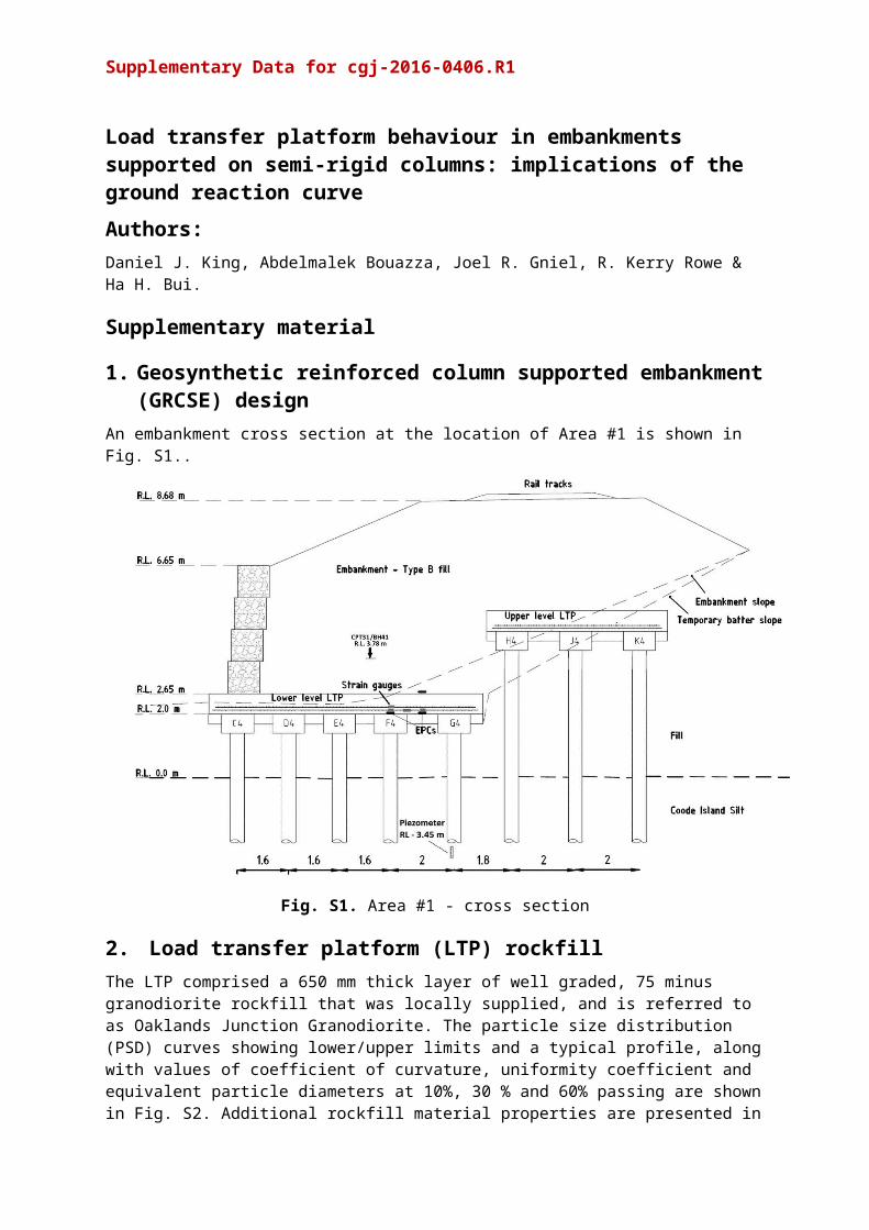
An embankment cross section at the location of Area #1 is shown in Fig. S1..
Fig. S1. Area #1 - cross section
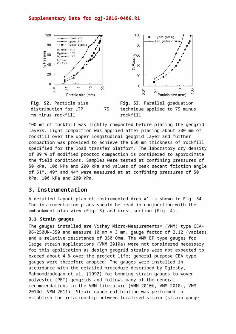
2. Load transfer platform (LTP) rockfillThe LTP comprised a 650 mm thick layer of well graded, 75 minus granodiorite rockfill that was locally supplied, and is referred to as Oaklands Junction Granodiorite. The particle size distribution (PSD) curves showing lower/upper limits and a typical profile, along with values of coefficient of curvature, uniformity coefficient and equivalent particle diameters at 10%, 30 % and 60% passing are shown in Fig. S2. Additional rockfill material properties are presented in Table S1. Due to difficulties finding a suitable sized direct shear box test apparatus owing to the large particle size of the rockfill, the parallel gradation technique originally developed by Lowe (1964) has been used to estimate the shear strength properties of the rockfill. The PSD for the 75 mm minus rockfill (typical curve) and for the scaled 26 mm minus rockfill tested is shown in Fig. S3.
The direct shear tests were performed on the scaled rockfill using the Monash University’s Constant Normal Stiffness direct shear apparatus (Haberfield and Szymakowski 2003). The shear box used has a plan area of 600 mm by 200 mm and height of 135 mm. The rockfill was compacted in the shear box in about 40 mm layers and the dry density was calculated to be 18.7 kN/m3. A target rockfill density was not specified in design in order to avoid damaging the geogrid layers. The bottom
Supplementary Data for cgj-2016-0406.R1
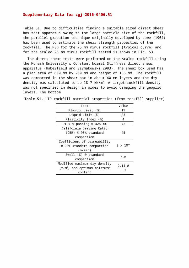
Table S1. LTP rockfill material properties (from rockfill supplier)
Test ValuePlastic Limit (%) 19Liquid Limit (%) 23
Plasticity Index (%) 4PI x % passing 0.425 mm 72
California Bearing Ratio (CBR) @ 98% standard compaction 45
Coefficient of permeability @ 98% standard compaction (m/sec)
2 x 10⁻⁸
Swell (%) @ standard compaction 0.0Modified maximum dry density (t/m3)
and optimum moisture content 2.14 @ 8.2
Fig. S2. Particle size distribution for LTP 75 mm minus rockfill
Fig. S3. Parallel graduation technique applied to 75 minus rockfill
100 mm of rockfill was lightly compacted before placing the geogrid layers. Light compaction was applied after placing about 300 mm of rockfill over the upper longitudinal geogrid layer and further compaction was provided to achieve the 650 mm thickness of rockfill specified for the load transfer platform. The laboratory dry density of 89 % of modified proctor compaction is considered to approximate the field conditions. Samples were tested at confining pressures of 50 kPa, 100 kPa and 200 kPa and values of peak secant friction angle of 51°, 49° and 44° were measured at at confining pressures of 50 kPa, 100 kPa and 200 kPa.
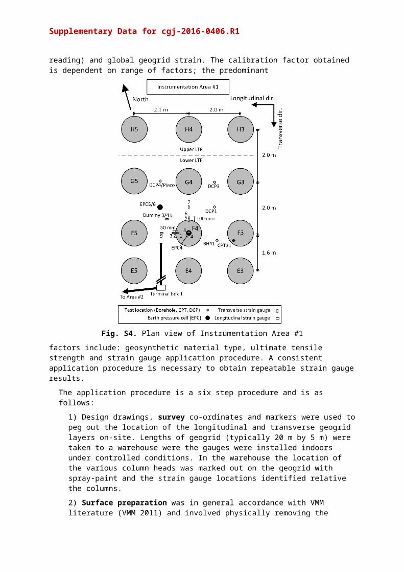
3. Instrumentation A detailed layout plan of instrumented Area #1 is shown in Fig. S4. The instrumentation plans should be read in conjunction with the embankment plan view (Fig. 3) and cross-section (Fig. 4).
3.1 Strain gaugesThe gauges installed are Vishay Micro-Measurements® (VMM) type CEA-06-250UN-350 and measure 10 mm × 3 mm, gauge factor of 2.12 (varies) and a relative resistance of 350 Ohm. The VMM EP type gauges for large strain applications (VMM 2010a) were not considered necessary for this application as design geogrid strains were not expected to exceed about 4 % over the project life; general purpose CEA type gauges were therefore adopted. The gauges were installed in accordance with the detailed procedure described by Oglesby, Mahmoodzadegan et al. (1992) for bonding strain gauges to woven polyester (PET) geogrids and follows many of the general recommendations in the VMM literature (VMM 2010b, VMM 2010c, VMM 2010d, VMM 2011). Strain gauge calibration was performed to establish the relationship between localised strain (strain gauge reading) and global geogrid strain. The calibration factor obtained is dependent on range of factors; the predominant
Supplementary Data for cgj-2016-0406.R1
Fig. S4. Plan view of Instrumentation Area #1
factors include: geosynthetic material type, ultimate tensile strength and strain gauge application procedure. A consistent application procedure is necessary to obtain repeatable strain gauge results.
The application procedure is a six step procedure and is as follows:
1) Design drawings, survey co-ordinates and markers were used to peg out the location of the longitudinal and transverse geogrid layers on-site. Lengths of geogrid (typically 20 m by 5 m) were taken to a warehouse were the gauges were installed indoors under controlled conditions. In the warehouse the location of the various column heads was marked out on the geogrid with spray-paint and the strain gauge locations identified relative the columns.
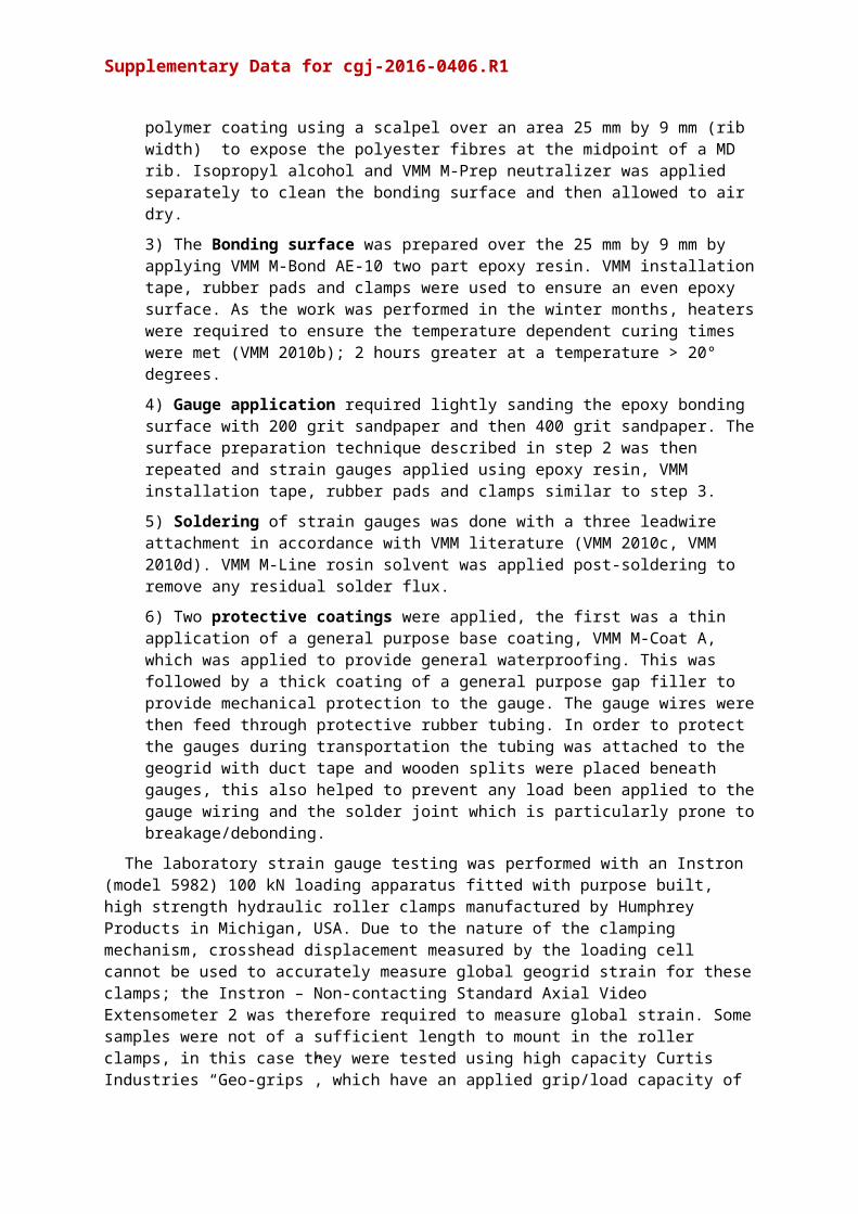
2) Surface preparation was in general accordance with VMM literature (VMM 2011) and involved physically removing the polymer coating using a scalpel over an area 25 mm by 9 mm (rib width) to expose the polyester fibres at the midpoint of a MD rib. Isopropyl alcohol and VMM M-Prep neutralizer was applied separately to clean the bonding surface and then allowed to air dry.
3) The Bonding surface was prepared over the 25 mm by 9 mm by applying VMM M-Bond AE-10 two part epoxy resin. VMM installation tape, rubber pads and clamps were used to ensure an even epoxy surface. As the work was performed in the winter months, heaters were required to ensure the temperature dependent curing times were met (VMM 2010b); 2 hours greater at a temperature > 20° degrees.
4) Gauge application required lightly sanding the epoxy bonding surface with 200 grit sandpaper and then 400 grit sandpaper. The surface preparation technique described in step 2 was then repeated and strain gauges applied using epoxy resin, VMM installation tape, rubber pads and clamps similar to step 3.
Supplementary Data for cgj-2016-0406.R1
5) Soldering of strain gauges was done with a three leadwire attachment in accordance with VMM literature (VMM 2010c, VMM 2010d). VMM M-Line rosin solvent was applied post-soldering to remove any residual solder flux.
6) Two protective coatings were applied, the first was a thin application of a general purpose base coating, VMM M-Coat A, which was applied to provide general waterproofing. This was followed by a thick coating of a general purpose gap filler to provide mechanical protection to the gauge. The gauge wires were then feed through protective rubber tubing. In order to protect the gauges during transportation the tubing was attached to the geogrid with duct tape and wooden splits were placed beneath gauges, this also helped to prevent any load been applied to the gauge wiring and the solder joint which is particularly prone to breakage/debonding.
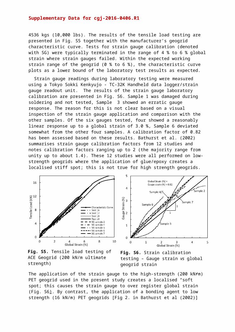
The laboratory strain gauge testing was performed with an Instron (model 5982) 100 kN loading apparatus fitted with purpose built, high strength hydraulic roller clamps manufactured by Humphrey Products in Michigan, USA. Due to the nature of the clamping mechanism, crosshead displacement measured by the loading cell cannot be used to accurately measure global geogrid strain for these clamps; the Instron – Non-contacting Standard Axial Video Extensometer 2 was therefore required to measure global strain. Some samples were not of a sufficient length to mount in the roller clamps, in this case they were tested using high capacity Curtis Industries “Geo-grips”, which have an applied grip/load capacity of 4536 kgs (10,000 lbs). The results of the tensile load testing are presented in Fig.S5 together with the manufacturer’s geogrid characteristic curve. Tests for strain gauge calibration (denoted with SG) were typically terminated in the range of 4 % to 6 % global strain where strain gauges failed. Within the expected working strain range of the geogrid (0 % to 6 %), the characteristic curve plots as a lower bound of the laboratory test results as expected.
Strain gauge readings during laboratory testing were measured using a Tokyo Sokki Kenkyujo - TC-32K Handheld data logger/strain gauge readout unit. The results of the strain gauge laboratory calibration are presented in Fig. S6. Sample 1 was damaged during soldering and not tested, Sample 3 showed an erratic gauge response. The reason for this is not clear based on a visual inspection of the strain gauge application and comparison with the other samples. Of the six gauges tested, four showed a reasonably linear response up to a global strain of 3.0 %, Sample 6 deviated somewhat from the other four samples. A calibration factor of 0.82 has been assessed based on these results. Bathurst et al. (2002) summarises strain gauge calibration factors from 12 studies and notes calibration factors ranging up to 2 (the majority range from unity up to about 1.4). These 12 studies were all performed on low-strength geogrids where the application of glue/epoxy creates a localised stiff spot; this is not true for high strength geogrids.
Fig. S6. Strain calibration testing – Gauge strain vs global geogrid strain
Supplementary Data for cgj-2016-0406.R1
The application of the strain gauge to the high-strength (200 kN/m) PET geogrid used in the present study creates a localised “soft” spot; this causes the strain gauge to over register global strain (Fig. S6). By contrast, the application of a bonding agent to low strength (16 kN/m) PET geogrids [Fig 2. in Bathurst et al (2002)] creates a “hard” spot and leads to strain gauge readings which under register global strain. The calibration factor obtained by the authors is consistent with Oglesby et al. (1992) who also applied strain gauges to a high-strength (133 kN/m) polyester (PET) geogrid.
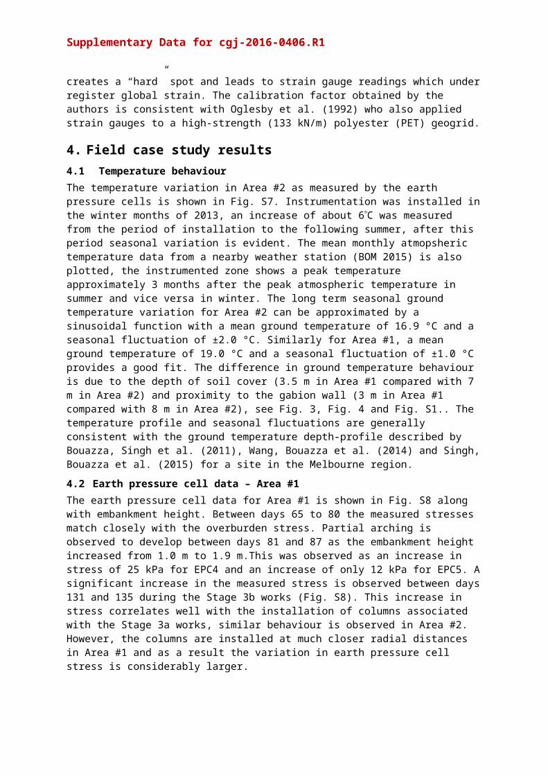
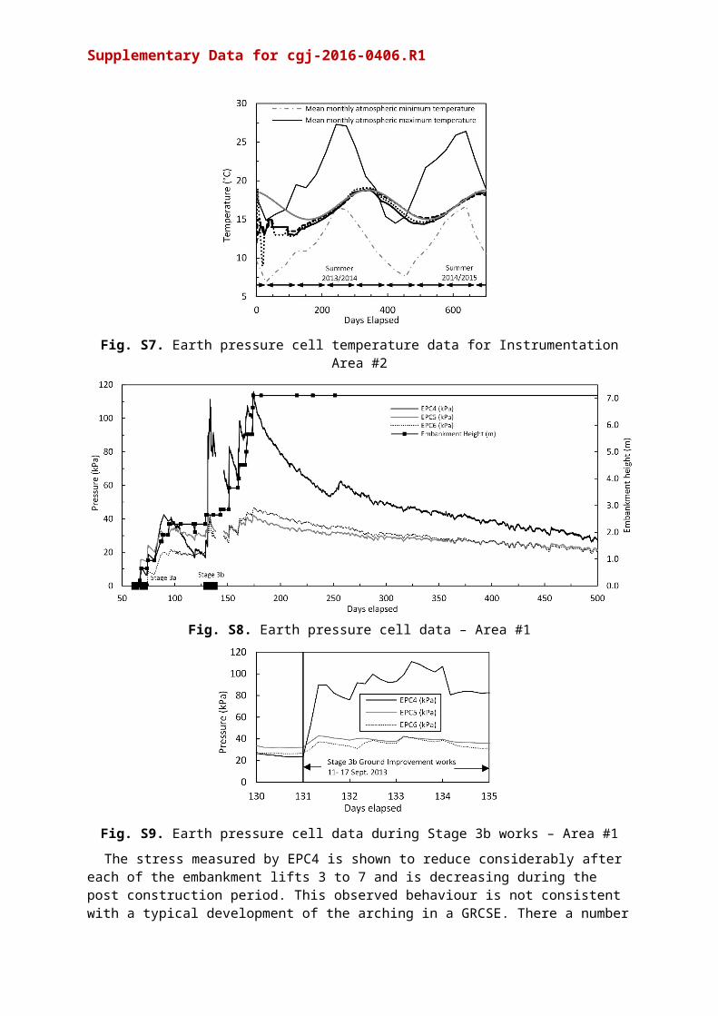
4. Field case study results4.1 Temperature behaviourThe temperature variation in Area #2 as measured by the earth pressure cells is shown in Fig. S7. Instrumentation was installed in the winter months of 2013, an increase of about 6C was measured from the period of installation to the following summer, after this period seasonal variation is evident. The mean monthly atmopsheric temperature data from a nearby weather station (BOM 2015) is also plotted, the instrumented zone shows a peak temperature approximately 3 months after the peak atmospheric temperature in summer and vice versa in winter. The long term seasonal ground temperature variation for Area #2 can be approximated by a sinusoidal function with a mean ground temperature of 16.9 °C and a seasonal fluctuation of ±2.0 °C. Similarly for Area #1, a mean ground temperature of 19.0 °C and a seasonal fluctuation of ±1.0 °C provides a good fit. The difference in ground temperature behaviour is due to the depth of soil cover (3.5 m in Area #1 compared with 7 m in Area #2) and proximity to the gabion wall (3 m in Area #1 compared with 8 m in Area #2), see Fig. 3, Fig. 4 and Fig. S1.. The temperature profile and seasonal fluctuations are generally consistent with the ground temperature depth-profile described by Bouazza, Singh et al. (2011), Wang, Bouazza et al. (2014) and Singh, Bouazza et al. (2015) for a site in the Melbourne region.
4.2 Earth pressure cell data – Area #1The earth pressure cell data for Area #1 is shown in Fig. S8 along with embankment height. Between days 65 to 80 the measured stresses match closely with the overburden stress. Partial arching is observed to develop between days 81 and 87 as the embankment height increased from 1.0 m to 1.9 m.This was observed as an increase in stress of 25 kPa for EPC4 and an increase of only 12 kPa for EPC5. A significant increase in the measured stress is observed between days 131 and 135 during the Stage 3b works (Fig. S8). This increase in stress correlates well with the installation of columns associated with the Stage 3a works, similar behaviour is observed in Area #2. However, the columns are installed at much closer radial distances in Area #1 and as a result the variation in earth pressure cell stress is considerably larger.
Fig. S7. Earth pressure cell temperature data for Instrumentation Area #2
Supplementary Data for cgj-2016-0406.R1
Fig. S8. Earth pressure cell data – Area #1
Fig. S9. Earth pressure cell data during Stage 3b works – Area #1
The stress measured by EPC4 is shown to reduce considerably after each of the embankment lifts 3 to 7 and is decreasing during the post construction period. This observed behaviour is not consistent with a typical development of the arching in a GRCSE. There a number of mechanisms that may cause this behaviour. Firstly, the possibility that EPC4 is not functioning correctly is considered. However, given the response of EPC4 during the embankment lifts and Stage 3a works it appears that the earth pressure cell is functioning correctly. It is thought that this behaviour is due to a “shadow” effect caused by the upper LTP, which is situated immediately adjacent to and above Area #1 (Fig. S1). As embankment lifts are constructed it is inferred that load within the embankment soil mass is distributed to the more rigid upper LTP. In effect, this causes a “virtual” reduction in the height of overburden material acting in Area #1. As partial arching is inferred to have developed above Area #1 prior to embankment lifts 3 to 7, this unloading of the overburden stress occurs primarily along the existing arching stress paths i.e. load component A (measured by EPC4 and to a lesser extent EPC6). The stress in the area between columns (measured by EPC5) shows only a minor reduction by comparison.
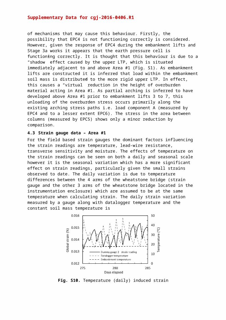
4.3 Strain gauge data – Area #1For the field based strain gauges the dominant factors influencing the strain readings are temperature, lead-wire resistance, transverse sensitivity and moisture. The effects of temperature on the strain readings can be seen on both a daily and seasonal scale however it is the seasonal variation which has a more significant effect on strain readings, particularly given the small strains observed to date. The daily variation is due to temperature differences between the 4 arms of the wheatstone bridge (strain gauge and the other 3 arms of the wheatstone bridge located in the instrumentation enclosure) which are assumed to be at the same temperature when calculating strain. The daily strain variation measured by a gauge along with datalogger temperature and the constant soil mass temperature is
Supplementary Data for cgj-2016-0406.R1
Fig. S10. Temperature (daily) induced strain
shown in Fig. S9. The variation in strain of about ±10 με (±0.001 % strain) averages out when viewed over a larger time-scale, and therefore has not been corrected for.
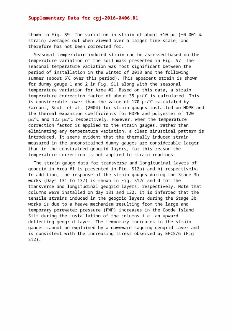
Seasonal temperature induced strain can be assessed based on the temperature variation of the soil mass presented in Fig. S7. The seasonal temperature variation was most significant between the period of installation in the winter of 2013 and the following summer (about 5C over this period). This apparent strain is shown for dummy gauge 1 and 2 in Fig. S11 along with the seasonal temperature variation for Area #2. Based on this data, a strain temperature correction factor of about 35 µ/C is calculated. This is considerable lower than the value of 170 µ/C calculated by Zarnani, Scott et al. (2004) for strain gauges installed on HDPE and the thermal expansion coefficients for HDPE and polyester of 120 µ/C and 123 µ/C respectively. However, when the temperature correction factor is applied to the strain gauges, rather than eliminating any temperature variation, a clear sinusoidal pattern is introduced. It seems evident that the thermally induced strain measured in the unconstrained dummy gauges are considerable larger than in the constrained geogrid layers, for this reason the temperature correction is not applied to strain readings.
The strain gauge data for transverse and longitudinal layers of geogrid in Area #1 is presented in Fig. S12a) and b) respectively. In addition, the response of the strain gauges during the Stage 3b works (Days 131 to 137) is shown in Fig. S12c and d for the transverse and longitudinal geogrid layers, respectively. Note that columns were installed on day 131 and 132. It is inferred that the tensile strains induced in the geogrid layers during the Stage 3b works is due to a heave mechanism resulting from the large and temporary porewater pressure (PWP) increases in the Coode Island Silt during the installation of the columns i.e. an upward deflecting geogrid layer. The temporary increases in the strain gauges cannot be explained by a downward sagging geogrid layer and is consistent with the increasing stress observed by EPC5/6 (Fig. S12).
Fig. S11. Temperature (seasonal) induced strain
Supplementary Data for cgj-2016-0406.R1
Due to the influence of the upper level ground improvement works and the upward deflection of the geogrid layer, it is somewhat more difficult to assess the long term behaviour of the geogrid. In addition, it is shown later in this paper that the subsoil settlement (to date) is quite small, resulting in only a small amount of geogrid strain. Of the transverse strain gauges, only gauges 5E and 5W develop realistic tensile strains, while gauges 6W and 7E measure either constant and/or compressive strains over the long term. Gauges 5E/5W indicate an average increase in tensile strain of about 0.04 % from day 150 through to day 300. Beyond this period the gauges are relatively stable. Of the longitudinal gauges, gauges 4S and 1N indicate increasing tensile strain of about 0.05 % between days 150 to 300. The remaining gauges are either constant and/or decreasing in strain over the long term, this may be due to the reduction in the tensile strains induced during the Stage 3b works.
On the basis of the results presented it is difficult to comment on the strain concentration described by Han and Gabr (2002), Jones, Plaut et al. (2010) and Zhuang and Wang (2015) other than to note that minimal strain was observed at the mid-span between columns (gauges 7E and 9S) and higher strain was observed to develop in the gauges located near the edge (gauges 1N, 5E and 5W) and centre of column heads (4S). Whilst these strain readings do not confirm the expected concentrated strains near the edge of the column head, the results do not contradict this behaviour either. Given the small amount of sub-soil settlement which is inferred to have occurred to date, more time is required for sub-soil settlement to occur and the GR behaviour (increased tensile load) to fully develop.
5. Overburden stressTo account for geometry of the embankment and the presence of the gabion wall, a 2D plain strain
finite element analysis was performed to more accurately assess the overburden stress (σv0) in Area #2. The embankment geometry is shown in Fig. S13 and material parameters adopted are outlined in
Fig. S12. Strain gauge data: (a) longitudinal geogrid, (b) transverse geogrid, (c) longitudinal Stage 3b works and (d) transverse Stage GI works.
Supplementary Data for cgj-2016-0406.R1
Table S2. The LTP zone is modelled as “rigid” with high stiffness and strength values in order to avoid the development of arching and allow the calculation of overburden stresses. Twelve embankment construction phases, each a function of embankment height, were modelled, allowing comparison of the earth pressure cell data at various stages of construction. This model was developed to assess stress distribution within the embankment soil mass and not intended for rigorous assessment of global and localised embankment behaviour which is covered in a separate paper.
6. Comparison with settlement analysisFor the settlement analysis of sub-soil in Area #2 the compressibility of the 2 m thick stiff to very-stiff fill layer, overlying the Coode Island Silt, is ignored under the low applied stresses acting in the area between columns; the settlement analysis is focused on assessing the time-dependent consolidation of the underlying Coode Island Silt. The applied stress acting on the upper surface of the Coode Island Silt is calculated from sub-soil stress (EPC2)(Fig. S14) and is approximated using a series of incremental loadings. The total applied stress acting on the Coode Island Silt has been calculated by assuming load spreading through the fill unit based on the ratio of the surface area between column heads, and the surface area at the upper surface of the Coode Island Silt (less the area of column shafts) a ratio of 4.0/4.9 is calculated from the Area #2 geometry (Fig. S15). The stress distribution with depth in the Coode Island Silt is calculated based on the embankment width (12 m) and a 2:1 method stress distribution. The Coode Island Silt is sub-divided into 3 sub-layers with the parameters adopted for the settlement analysis (Table 3) based on the laboratory testing described in King, Bouazza et al. (2016). The time-rate of settlement is assessed using the time-U(%) relationship described by Srithar (2010) which is back-calculated from field scale settlement data from Coode Island Silt sites.
Fig. S13. Embankment geometry for finite element analysis
Table S2. Material parameters for 2D plain strain finite element analysis
*M-C Mohr-Coulomb, †LE Linear elastic, ‡H-S Hardening soil
Supplementary Data for cgj-2016-0406.R1
Fig. S14. Applied loading acting on sub-soil for Area #2 settlement analysis
Fig. S15. Calculation of applied stress on upper surface of the Coode Island Silt
There are two factors which have a considerable effect on the calculated settlement presented in Fig. S16: 1) the time-rate of settlement parameters cv (coefficient of consolidation) and H (maximum drainage length) and 2) the long term creep consolidation. After about day 200 the applied stress reduces and consolidation occurs within the re-compression range; the rate of settlement reduces considerably. Longer term, under the small applied stresses of about 8 kPa, the sub-soil settlement is dominated by creep consolidation. The settlement analysis presented ignores the load transfer to the columns and the “ground improvement effect” in the Coode Island Silt due to the ground improvement works, as a result, the plotted settlement represents the upper bound of settlement with respect to time.
The variation in applied stress acting on the Coode Island Silt with depth in Fig. S17. The initial applied load at stress reduction ratio = 1.0 through to maximum arching (stress reduction ratio = 0.09) is shown along with the case of no ground improvement. Based on this assessment, only the upper few meters of Coode Island Silt is in the normally consolidated range, and this occurs only for a short period of time. The majority of the consolidation behaviour with depth occurs in the re-compression range. In the long term, however, creep compression dominates, particularly during the period of maximum arching where the applied stress acting on the sub-soil is measured to be just 8 kPa.
Fig. S16. Results of Area #2 settlement analysis Fig. S17. Applied stress acting on Coode Island Silt layer due to embankment construction
Supplementary Data for cgj-2016-0406.R1
7. ReferencesBOM (2015). Australian Government Bureau of Meteorology - Mean monthly maximum and
minimum temperature - Melbourne regional office weather station [Data set]. Retrieved from http://www.bom.gov.au/climate/data/stations/.
Bouazza, A., R. M. Singh, B. Wang, D. Barry-Macaulay, C. Haberfield, G. Chapman, S. Baycan and Y. Carden (2011). Harnessing on site renewable energy through pile foundations. Australian Geomechanics 46(4): pp. 79-90.
Haberfield, C. M. and J. Szymakowski (2003). Applications of large scale direct shear testing. Australian Geomechanics 38(1): pp. 29-39.
Han, J. and M. A. Gabr (2002). Numerical analysis of geosynthetic-reinforced and pile-supported earth platforms over soft soil. Journal of Geotechnical and Geoenvironmental Engineering 128(1): pp. 44-53.
Jones, B. M., R. H. Plaut and G. M. Filz (2010). Analysis of geosynthetic reinforcement in pile-supported embankments. Part I: 3D plate model. Geosynthetics International 17(2): pp. 59-67.
King, D. J., A. Bouazza, J. Gniel and H. H. Bui (2016). The compressibility, permeability and structured nature of the Coode Island Silt. Australian Geomechanics 50(2): pp. 45-62.
Lowe, J. (1964). Shear strength of coarse embankment dam materials. 8th International Congress on Large Dams, Edinburgh, Scotland, International Commission on Large Dams.
Oglesby, J. W., B. Mahmoodzadegan and P. M. Griffin (1992). Evaluation of methods and materials used to attach strain gages to polymer grids for high strain conditions. Louisiana Transportation Research Center. Baton Rouge, LA.
Singh, R. M., A. Bouazza and B. Wang (2015). Near-field ground thermal response to heating of a geothermal energy pile: Observations from a field test. Soils and Foundations("In press").
Srithar, S. T. (2010). Settlement characteristics of Coode Island Silt. Australian Geomechanics 45(1): pp. 55-64.
VMM (2010b). Vishay Micro Measurements. Instructional Bulletin B-137. Strain gage applications with M-Bond AE-10, AE-15 and GA-2 adhesive systems. Available from http://www.vishaypg.com/micro-measurements/stress-analysis-strain-gages/instruction-list/. [accessed 4 December 2015]
VMM (2010c). Vishay Micro Measurements. Application Note TN-609 Strain gage soldering techniques. Available from http://www.vishaypg.com/micro-measurements/stress-analysis-strain-gages/appnotes-list/. [accessed 4 December 2015].
VMM (2010d). Vishay Micro Measurements. Application Note VMM-21 Three leadwire attachment. Available from http://www.vishaypg.com/micro-measurements/stress-analysis-strain-gages/appnotes-list/. [Accessed 4 December 2015].
VMM (2011). Vishay Micro Measurements. Instruction Bulletin B-129-8. Surface Preparation for strain gage bonding. Available from http://www.vishaypg.com/micro-measurements/stress-analysis-strain-gages/instruction-list/. [accessed 4 December 2015].
Wang, B., A. Bouazza, R. M. Singh, C. Haberfield, D. Barry-Macaulay and S. Baycan (2014). Posttemperature Effects on Shaft Capacity of a Full-Scale Geothermal Energy Pile. Journal of Geotechnical and Geoenvironmental Engineering 141(4).
Zarnani, S., J. D. Scott and D. C. Sego (2004). Long term performance of geogrid strain gauges. 57th Canadian Geotechnical Conference, Québec City, Québec.
Zhuang, Y. and K. Y. Wang (2015). Three-dimensional behavior of biaxial geogrid in a piled embankment: numerical investigation. Canadian Geotechnical Journal 52: pp. 1629-1635.