For More Information Visit RAND at www.rand.org Explore the Pardee RAND Graduate School View document details Support RAND Browse Reports & Bookstore Make a charitable contribution Limited Electronic Distribution Rights is document and trademark(s) contained herein are protected by law as indicated in a notice appearing later in this work. is electronic representation of RAND intellectual property is provided for non- commercial use only. Unauthorized posting of RAND electronic documents to a non-RAND website is prohibited. RAND electronic documents are protected under copyright law. Permission is required from RAND to reproduce, or reuse in another form, any of our research documents for commercial use. For information on reprint and linking permissions, please see RAND Permissions. Skip all front matter: Jump to Page 16 e RAND Corporation is a nonprofit institution that helps improve policy and decisionmaking through research and analysis. is electronic document was made available from www.rand.org as a public service of the RAND Corporation. CHILDREN AND FAMILIES EDUCATION AND THE ARTS ENERGY AND ENVIRONMENT HEALTH AND HEALTH CARE INFRASTRUCTURE AND TRANSPORTATION INTERNATIONAL AFFAIRS LAW AND BUSINESS NATIONAL SECURITY POPULATION AND AGING PUBLIC SAFETY SCIENCE AND TECHNOLOGY TERRORISM AND HOMELAND SECURITY
Transcript
For More InformationVisit RAND at www.rand.org
Explore the Pardee RAND Graduate School
View document details
Support RANDBrowse Reports & Bookstore
Make a charitable contribution
Limited Electronic Distribution RightsThis document and trademark(s) contained herein are protected by law as indicated in a notice appearing later in this work. This electronic representation of RAND intellectual property is provided for non-commercial use only. Unauthorized posting of RAND electronic documents to a non-RAND website is prohibited. RAND electronic documents are protected under copyright law. Permission is required from RAND to reproduce, or reuse in another form, any of our research documents for commercial use. For information on reprint and linking permissions, please see RAND Permissions.
Skip all front matter: Jump to Page 16
The RAND Corporation is a nonprofit institution that helps improve policy and decisionmaking through research and analysis.
This electronic document was made available from www.rand.org as a public service of the RAND Corporation.
This product is part of the Pardee RAND Graduate School (PRGS) dissertation series.
PRGS dissertations are produced by graduate fellows of the Pardee RAND Graduate
School, the world’s leading producer of Ph.D.’s in policy analysis. The dissertation has
been supervised, reviewed, and approved by the graduate fellow’s faculty committee.
C O R P O R A T I O N
Dissertation
Three Essays on Subjective Well-Being
Caroline Tassot
Dissertation
Three Essays on Subjective Well-Being
Caroline Tassot
This document was submitted as a dissertation in May 2014 in partial fulfillment of the requirements of the doctoral degree in public policy analysis at the Pardee RAND Graduate School. The faculty committee that supervised and approved the dissertation consisted of Arie Kapteyn (Chair), Richard Easterlin, and Susann Rohwedder.
PARDEE RAND GRADUATE SCHOOL
The RAND Corporation is a nonprofit institution that helps improve policy and decisionmaking through research and analysis. RAND’s publications do not necessarily reflect the opinions of its research clients and sponsors.
R® is a registered trademark.
Permission is given to duplicate this document for personal use only, as long as it is unaltered and complete. Copies may not be duplicated for commercial purposes. Unauthorized posting of RAND documents to a non-RAND website is prohibited. RAND documents are protected under copyright law. For information on reprint and linking permissions, please visit the RAND permissions page (http://www.rand.org/publications/permissions.html).
Published 2014 by the RAND Corporation1776 Main Street, P.O. Box 2138, Santa Monica, CA 90407-2138
1200 South Hayes Street, Arlington, VA 22202-50504570 Fifth Avenue, Suite 600, Pittsburgh, PA 15213-2665
RAND URL: http://www.rand.org/To order RAND documents or to obtain additional information, contact
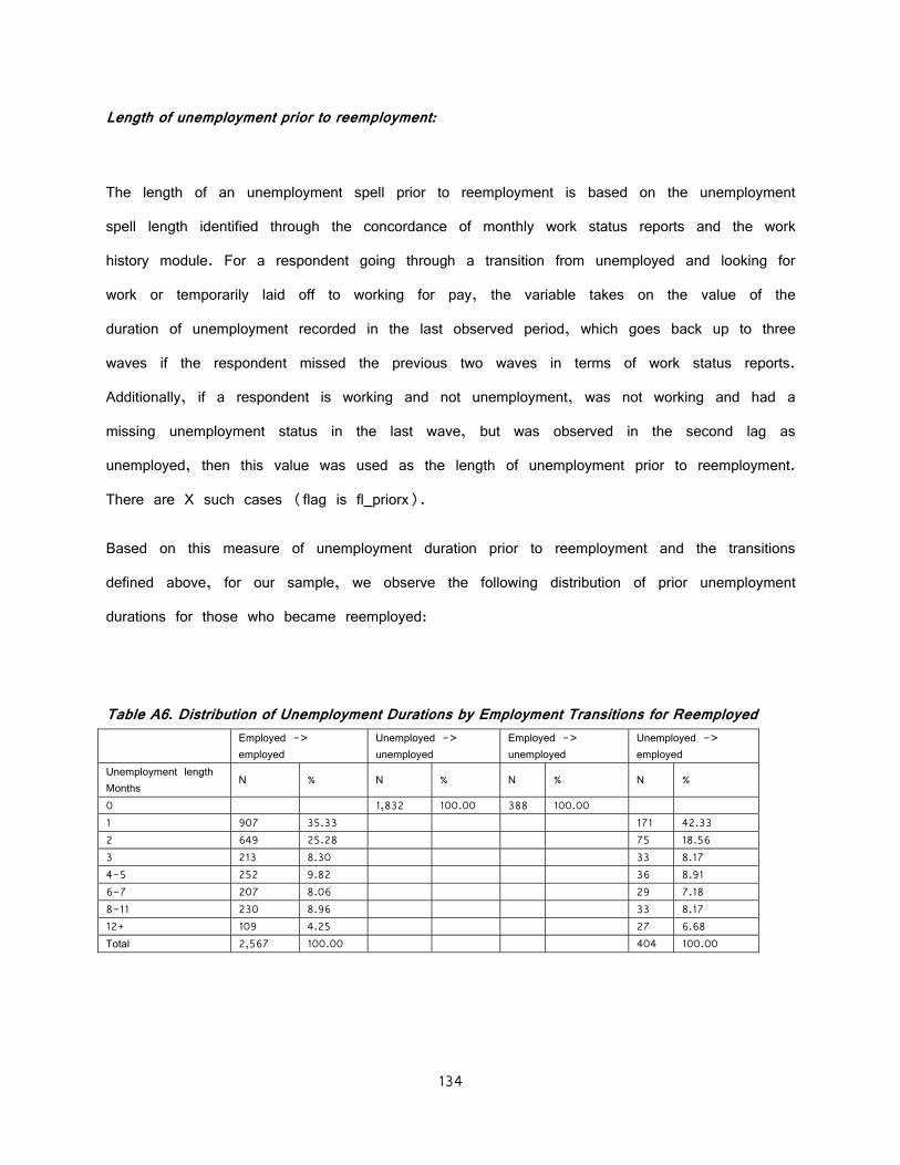
The Impact of Employment Transitions on Subjective Well-being: Evidence from the Great Recession and its Aftermath ..................................................................................... 52
Income Inequality and Subjective Well-Being: Evidence from the United States during the Great Recession ............................................................................................................ 145
1. Literature Review............................................................................................ 148
Income and Subjective Well-Being ...................................................................... 148
Income Inequality and Subjective Well-being ......................................................... 150
2. Methodology and Approach .............................................................................. 153
Data Sources ................................................................................................. 153
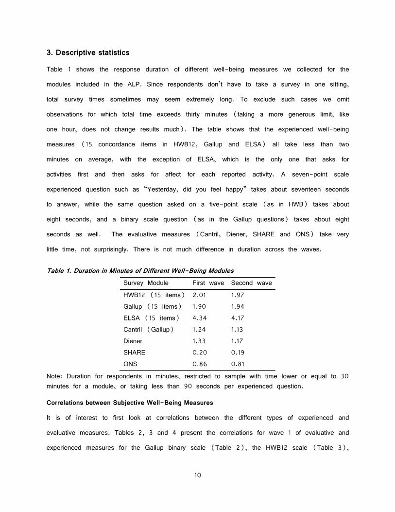
Note: Duration for respondents in minutes, restricted to sample with time lower or equal to 30 minutes for a module, or taking less than 90 seconds per experienced question.
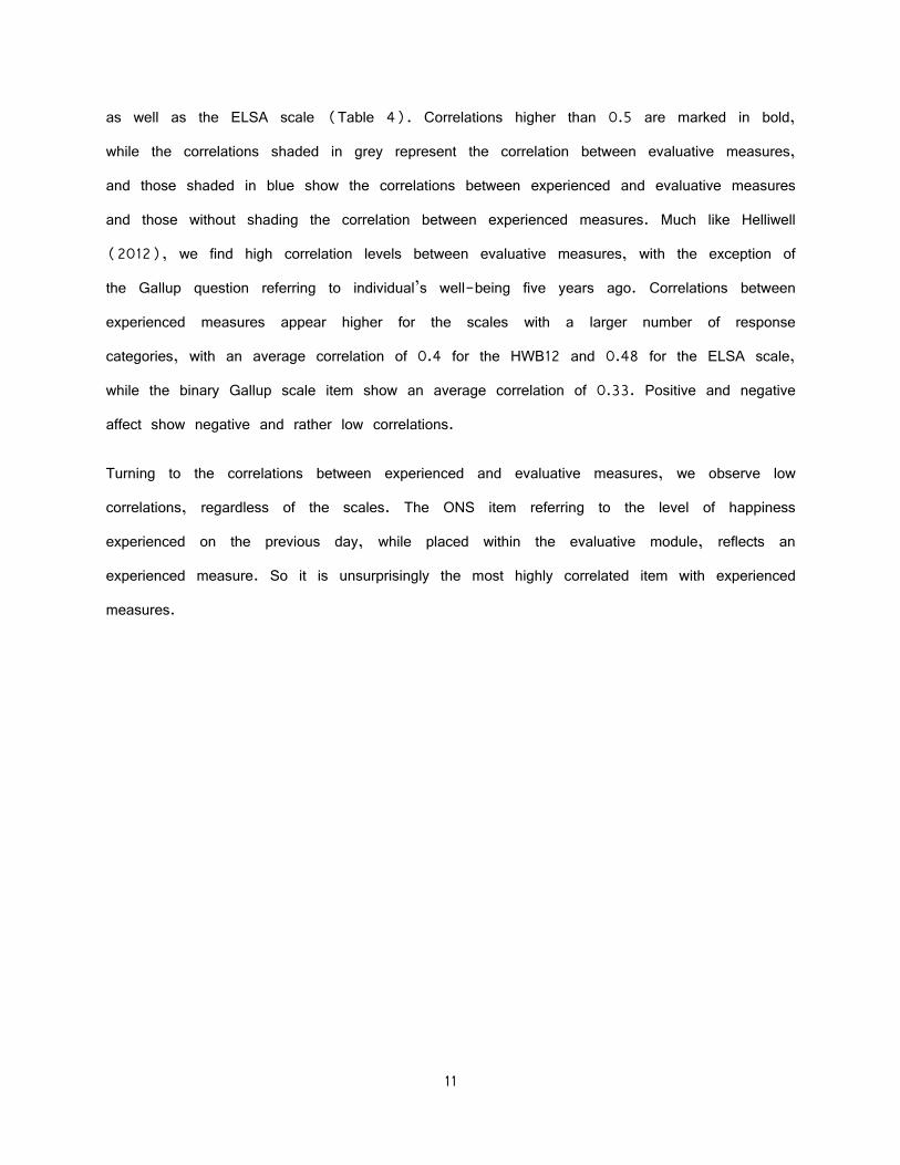
Correlations between Subjective Well-Being Measures
It is of interest to first look at correlations between the different types of experienced and
evaluative measures. Tables 2, 3 and 4 present the correlations for wave 1 of evaluative and
experienced measures for the Gallup binary scale (Table 2), the HWB12 scale (Table 3),
11
as well as the ELSA scale (Table 4). Correlations higher than 0.5 are marked in bold,
while the correlations shaded in grey represent the correlation between evaluative measures,
and those shaded in blue show the correlations between experienced and evaluative measures
and those without shading the correlation between experienced measures. Much like Helliwell
(2012), we find high correlation levels between evaluative measures, with the exception of
the Gallup question referring to individual’s well-being five years ago. Correlations between
experienced measures appear higher for the scales with a larger number of response
categories, with an average correlation of 0.4 for the HWB12 and 0.48 for the ELSA scale,
while the binary Gallup scale item show an average correlation of 0.33. Positive and negative
affect show negative and rather low correlations.
Turning to the correlations between experienced and evaluative measures, we observe low
correlations, regardless of the scales. The ONS item referring to the level of happiness
experienced on the previous day, while placed within the evaluative module, reflects an
experienced measure. So it is unsurprisingly the most highly correlated item with experienced
measures.
12
Table 2. Correlations between evaluative and Gallup experienced measures
G now
G 5 ago
G 5 Future
D ideal life
D Excellent conditions
D Satisfied
D im
portant things
D change life
SHARE Sat Life
ONS Sat now
ONS Happy
ONS Anxious
ONS worthwhile
Happy
Interested
Content
Joyful
Enthusiastic
Frustrated
Sad
Angry
Tired
Stressed
Lonely
Worried
Bored
Pain
Dep
ressed
G now 1.0
G 5 ago 0.4 1.0
G 5 Future 0.6 0.1 1.0
D ideal life 0.7 0.2 0.5 1.0
D Excellent Conditions 0.7 0.2 0.5 0.8 1.0
D Satisfied 0.7 0.2 0.5 0.8 0.8 1.0
D important things 0.6 0.3 0.4 0.7 0.6 0.7 1.0
D change life 0.5 0.2 0.4 0.6 0.6 0.6 0.6 1.0
SHARE Sat Life ‐0.7 ‐0.2 ‐0.5 ‐0.7 ‐0.7 ‐0.7 ‐0.6 ‐0.5 1.0
ONS Sat now 0.8 0.3 0.6 0.7 0.7 0.8 0.6 0.5 ‐0.8 1.0
An important question of interest when fielding a survey on subjective well-being questions is
the reliability of the resulting measures. We follow Krueger and Schkade (2008), and use a
classical measurement error model y_i=y_i^*+ ϵ_i, where y_i is the observed well-being item
measure, y_i^* is the true value of the well-being item measure and ϵ_i is an error term
assumed to have expectation zero. This set-up suggests a definition of the reliability ratio as
the correlation coefficient of measures across waves ( ), where the superscripts refer to the
waves in which the variables are measured. The reliability is thus measured here as a test-
retest correlation between two waves of data, where the interval in our sample is at least two
weeks.
Table 5 shows the reliability ratios for all the evaluative subjective well-being measures.
Overall, we observe that the Diener Satisfaction With Life Scale shows a reliability of about
0.80, which is very close to the estimate of 0.82 by Diener et al. (1985) who used an
interval of 2 months, and the estimate by Alfonso et al. (1996) of 0.83, where the interval
was two weeks between both measurements. As one would expect, the single item scales for
evaluative well-being yield somewhat lower correlations, on the order of 0.67. The two ONS
questions about yesterday are really experienced measures, as discussed earlier and we
observe lower correlations reflecting that the specific reference to “yesterday” should pick up
real changes in affect between different days. The Gallup measures referring to five years ago
or five years in the future show lower reliability ratios than the one referring to the present,
indicating possible error in recall of one’s situation five years ago and uncertainty about one’s
future.
16
Table 5. Reliability Ratio of the Evaluative Subjective Well-Being Measures. (n=3938) Satisfaction With Life Scale In most ways, my life is close to ideal. 0.68 The conditions of my life are excellent. 0.72 I am satisfied with my life. 0.73 So far I have gotten the important things I want in life. 0.67 If I could live my life over, I would change almost nothing. 0.65 Diener scale2 0.79 SHARE How satisfied are you with your life in general? 0.67 Gallup On which step of the ladder would you say you stood five years ago? 0.59 On which step of the ladder would you say you stand now? 0.71 On which step of the ladder would you say you will stand on in the future, say about five years from
now 0.66
ONS Overall, how satisfied are you with your life nowadays? 0.74 Overall, how happy did you feel yesterday? 0.57 Overall, how anxious did you feel yesterday? 0.45 Overall, to what extent do you feel that the things you do in your life are worthwhile? 0.65
We also looked at correlations between the measures for experienced affect on the previous
day presented in Table 6. As expected, we found lower correlations between waves, since
changes may reflect both random measurement errors and true changes between the two days
which the affect measures refer to. Notice that the table shows correlations for all items, i.e.
we include both the original items of each scale and the items added from the other scales.
Recall that we did this so that we are able to compare response scale effects across a
common set of items. (We have indicated the additional items by underlining the
correlations). Thus, a point of interest is to relate differences in correlations to differences in
response scales (both the wording and the number of points on the scale).
2 Computed as the average of the five Satisfaction With Life Items.
Note: Underlined correlations refer to items that have been added to the original scale;
correlations in bold indicate the highest and lowest values in each column.
The binary scale used in the Gallup survey shows somewhat lower correlations across waves
overall, with correlations between 0.28 and 0.49, in comparison with the five and six point
scales used in the HWB-12 and ELSA questionnaires respectively. The ELSA scale shows
correlations ranging from 0.33 to 0.55, while the HWB12 scale shows correlations between
.42 and .59.
4. The Relation between Evaluative and Experienced Well-Being Measures
There is a lively debate in the literature on the dimensions of well-being and what different
measures are capturing (for a review, see Diener, 2000). Uniquely, our data bring together
many of the currently used subjective well-being measures and thus allow us to investigate
how they are related. To determine the relation between the various measures we conducted
a number of different factor analyses.
18
As noted, we have all evaluative measures for all respondents, but each experienced measure
is only available for a randomly chosen five ninth of the sample. In their original form, the
Gallup and HWB12 measures are straightforward to use, since they produce ratings of a
number of affect items. The ELSA questionnaire is more complicated to analyze as it asks for
ratings for a number of activities during the previous day. We concentrate therefore initially on
analyses of the Gallup and HWB12 measures. The ELSA scale will be evaluated when
studying the concordance items, which can be found in all three experienced well-being
models. Both analyses cover all evaluative measures as well as their respective experienced
measures. We performed a factor analysis using principal components. In all cases factors are
rotated orthogonally using the varimax method while we retain factors with eigenvalues greater
than one3.
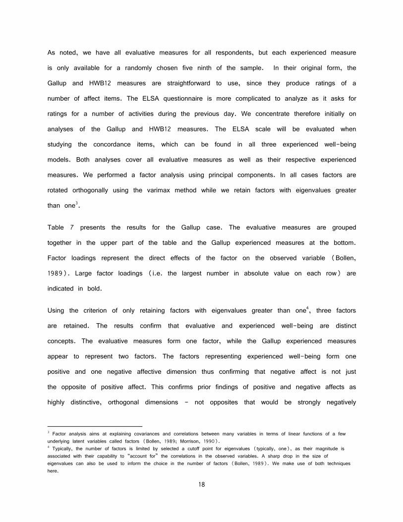
Table 7 presents the results for the Gallup case. The evaluative measures are grouped
together in the upper part of the table and the Gallup experienced measures at the bottom.
Factor loadings represent the direct effects of the factor on the observed variable (Bollen,
1989). Large factor loadings (i.e. the largest number in absolute value on each row) are
indicated in bold.
Using the criterion of only retaining factors with eigenvalues greater than one4, three factors
are retained. The results confirm that evaluative and experienced well-being are distinct
concepts. The evaluative measures form one factor, while the Gallup experienced measures
appear to represent two factors. The factors representing experienced well-being form one
positive and one negative affective dimension thus confirming that negative affect is not just
the opposite of positive affect. This confirms prior findings of positive and negative affects as
highly distinctive, orthogonal dimensions - not opposites that would be strongly negatively
3 Factor analysis aims at explaining covariances and correlations between many variables in terms of linear functions of a few underlying latent variables called factors (Bollen, 1989; Morrison, 1990). 4 Typically, the number of factors is limited by selected a cutoff point for eigenvalues (typically, one), as their magnitude is associated with their capability to “account for” the correlations in the observed variables. A sharp drop in the size of eigenvalues can also be used to inform the choice in the number of factors (Bollen, 1989). We make use of both techniques here.
19
correlated - so that individuals can be experiencing both positive and negative affect
simultaneously (Watson et al., 1988, Tuccitto et al., 2010). ONS-happy (Overall, how
happy did you feel yesterday?) loads mainly on the evaluative first factor. Although the
phrasing of the question would squarely put it in the experienced well-being domain, its
location in the survey (right after an evaluative question, see Appendix) may have induced
some respondents to use a global evaluation rather than focusing on yesterday’s affect.
Notably, ONS_worthwhile (“Overall, to what extent do you feel that the things you do in your
life are worthwhile?”) does not appear to represent a different factor from the evaluative
well-being factor. ONS-anxious loads on the negative affect factor, but with a surprising
Satisfied 0.8684 -0.2143 0.1467 Important things 0.7741 -0.0999 0.1444 Change life 0.7020 -0.0984 0.0280 SHARE Satisfaction w life 0.7953 -0.2094 0.1600 ONS Satisfied nowadays 0.8574 -0.2373 0.1868 Happy 0.6055 -0.4860 0.3437 Anxious -0.2000 0.0660 -0.6268 Worthwhile 0.6754 -0.3098 0.0896 Gallup Five years ago 0.3736 0.1720 0.2331 Now 0.8461 -0.2013 0.2029 Five years in future 0.6494 -0.2589 0.0018
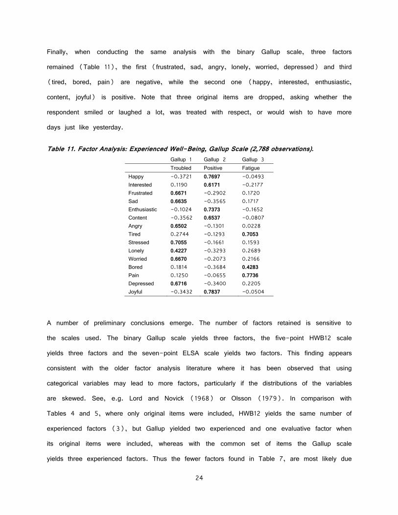
A number of preliminary conclusions emerge. The number of factors retained is sensitive to
the scales used. The binary Gallup scale yields three factors, the five-point HWB12 scale
yields three factors and the seven-point ELSA scale yields two factors. This finding appears
consistent with the older factor analysis literature where it has been observed that using
categorical variables may lead to more factors, particularly if the distributions of the variables
are skewed. See, e.g. Lord and Novick (1968) or Olsson (1979). In comparison with
Tables 4 and 5, where only original items were included, HWB12 yields the same number of
experienced factors (3), but Gallup yielded two experienced and one evaluative factor when
its original items were included, whereas with the common set of items the Gallup scale
yields three experienced factors. Thus the fewer factors found in Table 7, are most likely due
25
to the limited number of items included, as for instance boredom, fatigue, pain and loneliness
are missing from the original Gallup scale and indeed these contribute substantially to factor 3
in Table 11.
Factor analyses were also conducted on the common set of items, including evaluative
measures (not shown here). The results in terms of the number of factors emerging remain
quite similar, with one evaluative and two (three) experienced factor when using the ELSA
(HWB) scale, though it is worthwhile noticing that the ONS anxiety measure loads positively
on the negative experienced factors rather than on the evaluative factor. In the Gallup case a
fourth experienced factor (eigenvalue of 0.98) emerges representing mainly stress and pain.
Interpreting the larger number of factors as an artefact of the cruder scales suggests that first
of all it is advisable to use a scale with a fairly large number of response categories, e.g. 7
as in the ELSA scale. In that case, experienced well-being can be described by three
dimensions, one positive and two negative.
6. Relation with Individual Characteristics
While an extensive literature exists on the determinants of evaluative well-being (see for
example Dolan, Peasgood and White, 2008), much less is known of the determinants of
experienced well-being. We concentrate here on demographic and socio-economic
determinants. The motivation for this is that these appear most amenable to policy (e.g. with
respect to income, work, education, or childcare), while there is a general interest in
exploring how well-being varies with age, family composition (Deaton and Stone, 2013) and
gender. Furthermore it is of interest to explore to which extent determinants of evaluative
well-being are different from those of experienced well-being and whether the different
dimensions of experienced well-being have different determinants. We investigate how the
well-being measures are related to demographic variables, including race, gender, education
level, age bracket, having a partner, as well as socio-economic variables such as income
26
bracket and working status, while we also include self-reported health and number of children
in the household in our model. Formally, we specify the following model:
where is a vector of covariates, while ϵ_it represents random error uncorrelated with the
observable covariates. The subscript t indicates the wave (1 or 2) and i indexes the
respondent. The model is estimated by ordinary least squares, where we allow for correlation
of ϵ_it across the two waves (t=1 or t=2) by clustering standard errors on individuals5. The
simple equation specified here is not meant to provide a complete model of determinants of
well-being and indeed one can imagine that causality sometimes runs from well-being to
some of the right hand side variables. It is of interest nevertheless to investigate if the well-
being measures covary with other variables in a plausible manner and to see if the relation
between well-being and the right hand side variables is the same for each measure.
Table 12 shows the results for the evaluative measures. We have omitted the Gallup
measures for five years ago and five years in the future; similarly for ONS we have only
included the one true evaluative measure “Satisfied”. Given the different reference time frame
used by those Gallup items and the experienced and eudemonic measures of the ONS scale,
we chose to include only items referring to the present and involving evaluative measures.
Looking at the effects of gender, we observe that these vary by outcome measure and are
mostly insignificant. Men are less likely than women to agree with the statement “If I could
live my life again, I would change almost nothing”. There currently is no consensus in the
literature on the nature of differences in subjective well-being by sex, as some studies have
shown higher levels of happiness for men (Haring et al., 1984) which could be related to
higher prevalence of depression in women than men (Diener et. al., 1999), while others
have found that women report higher happiness (Alesina et al., 2004), and yet other
studies have found no evidence of gender effects on subjective well-being (Louis and Zhao,
5 Alternatively, we could have estimated a Random Effects model; the results of that specification are virtually indistinguishable from the results we obtain with the current specification.
27
2002; Dolan et al., 2008). Interactions between gender and education, income and having a
partner did not yield any statistically significant results. Having a partner increases life
satisfaction according to all measures. This result has also been found by others in the
literature (see e.g. Dolan et al., 2008; Blanchflower and Oswald, 2004). The presence of
children in the household does not seem to consistently affect the well-being of the
respondent, though as pointed out by Deaton and Stone (2013), this could be a function of
controlling for factors associated with having children, such as being married, richer, and
healthier. The results also show that by and large Blacks and Hispanics report higher
subjective well-being than non-Hispanic Whites. Concerning education, the reference category
for the education variables is “graduate education”. Although many coefficients are not
statistically significantly different from zero, all significant coefficients confirm Oswald and
Blanchflower’s finding of a positive relationship between education and well-being (2004).
Subjective well-being increases monotonically with income according to all evaluative measures.
In comparison to the reference category of respondents reporting an income above $100,000,
we observe large negative and statistically significant coefficients for most lower income groups.
The size of those coefficients suggests an almost linear relationship between income and
subjective well-being measures in this income range. A positive relation between income and
subjective well-being has been found many times in the literature, with existing research
suggesting positive but diminishing returns to income (Dolan et al., 2008).
The reference category for age consists of respondents over 65. Several studies have
suggested a “U-shape” in age with the lowest life satisfaction occurring in middle age
(Dolan et al., 2008; Blanchflower and Oswald, 2004). By and large that pattern is
confirmed for the various well-being measures in the table. We observe that self-reported
health – here coded as 1 being Excellent, and 5 Poor so that a negative sign represents a
higher level of health - is strongly correlated with well-being, which corresponds to general
findings in the literature (Diener et al., 1999; Helliwell, 2003).
28
With regards to working status, we used the category “working now” as a reference group,
so that the results for individuals who are retired, disabled, unemployed, or in a different
working situation (homemakers, or on sick leave, temporarily laid-off or other) represent
differences with “working now”. Consistent with the literature, we observe a strong negative
effect of being unemployed (see for instance Clark and Oswald (1994), Stutzer (2004) or
Di Tella et al (2001)). We also find a negative effect for being disabled, which appears in
line with studies challenging the theory of hedonic adaptation whereby individuals suffering
major changes in life circumstances, such as the onset of a disability, return to baseline
levels of happiness (Lucas, 2007). We also confirm prior findings (Kim and Moen, 2002)
of a strong positive relation between being retired and subjective well-being. Being in “Other
work” has a positive, though not always significant, effect on subjective well-being.
Finally, the last five rows show the p-values of joint significance tests for each category of
characteristics. We cannot reject the hypothesis of no difference between the education
categories except for the question “So far, I have gotten the important things I want in life”.
Virtually all other categories are jointly significant.
29
Table 12 . Regression of Evaluative Well-Being Measure on Demographic and SES Variables
Gallup Diener Diener scale ONS SHARE
Ideal life Excellent cond. Satisfied Important things Change life Factor Average Satisfied Satisfied
Notes: Observations are clustered at the individual level. The p-values mentioned in the last rows refer to a test of joint significance of the indicator variables for the categories race, education, income, age, and work status.
30
The coefficients in Table 13 are not directly comparable across columns as the dependent
variables are measured on different scales. However if the scales would be the only difference
between the dependent variables, then coefficients in different columns should be fixed
multiples of each other. Table 13 summarizes the results of tests of proportionality of
coefficients across the various models in Table 12 . The Null Hypothesis for all the tests is
formulated as follows: . The entries in the table are the p-values of
tests of the null hypothesis for each of the pairs of models that we are considering. We
observe that out of all ten possible combinations, the Null Hypothesis of proportionality of
coefficients gets rejected at the 5% level four times. All four rejections involve either the
Diener scale based on averaging the item scores or the Diener scale based on factor
analysis6. Inspecting the five items that constitute the Diener scale makes it clear that only
one item (“I am satisfied with my life”) corresponds with the simple one shot questions of
SHARE, ONS, and Gallup. This suggests that the Diener scale measures a somewhat broader
concept of evaluative well-being than the other three measures. Yet, remarkably in the factor
analyses presented earlier, it appeared that the items on the Diener scale all loaded on the
same overall satisfaction scale.
Table 13. Testing the Proportionality of Coefficients – Evaluative Measures (p-values) Gallup now Diener factor Diener average ONS Satisfaction
Diener factor 0.01 Diener average 0.01 0.09 ONS Satisfaction 0.89 0.02 0.02 SHARE Satisfaction 0.52 0.35 0.32 0.67
* The Null Hypothesis tested here is therefore testing the proportionality of coefficients across pairs of models. The table shows p-values of the test statistics corresponding to the null hypothesis for each pair of models.
6 Factor analysis of the Diener items yields one factor with eigenvalue greater than one (the eigenvalue equals 3.69)
H0
:
1,model1
1,model2
2,model1
2,model2
3,model1
3,model2
, etc.
H0
:
1,model1
1,model2
2,model1
2,model2
3,model1
3,model2
, etc.
31
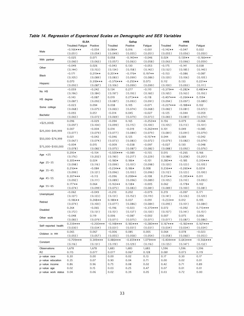
Table 14 shows the results of regressions where the dependent variables are scales based on
factor loadings from factor analyses presented in Tables 9-11. So in all cases the scales are
based on the common set of items. It is of interest to not only compare the scales (which
are only different because of differences in response scales), but also between the
experienced scales and the evaluative scales, for which regressions were presented in Table
12 . For both the ELSA and HWB12 scales males score lower on the negative affect
(“Troubled”) scale (but marginally significantly positive for the Gallup scale). Here again,
interactions between gender and education, income and having a partner did not yield any
statistically significant results. Having a partner has little effect on experienced well-being
(although the HWB12 scale suggests a somewhat lower score on the “Fatigue” scale), in
contrast to the findings for the evaluative well-being scales where the presence of a partner
has a strong positive effect.
The effect of ethnicity is hard to summarize. According to the ELSA scale Hispanics and
Blacks experience more positive affect compared to whites and non-Hispanic whites. According
to the Gallup scales Blacks and Hispanics experience less positive affect, while the HWB12
scale shows no significant effects of ethnicity on positive affect. For blacks we find more
negative affect for the Gallup scale. Hispanics are less troubled according to the Gallup scale
and more tired according to the HWB12 scale. Education also shows patterns that vary by
response scale. The ELSA and Gallup scales show few significant effects. The HWB12 scale
suggests that individuals with lower education experience less positive affect, while they are
also less troubled, but more tired, bored and suffering from pain.
The most striking contrast between evaluative and experienced well-being is the effect of
income. Whereas for evaluative well-being we observe a strong positive relation with income,
such a relation is hardly discernible for experienced well-being. This result is somewhat
stronger than earlier findings by Kahneman and Deaton (2010), who found that while life
evaluation items rise steadily with socio-economic status, experienced measures of well-being
do not improve beyond an annual income of approximately $75,000. Here we find very little
32
evidence of a relation with income, although interestingly the Gallup scale produces marginally
significant effects, which also is the scale used by Kahneman and Deaton (2010). Similarly,
we observe that the U-shaped relation with age that we observed for evaluative well-being
does not show up for experienced well-being. The results for labor market status show few
consistent patterns across scales. As with evaluative well-being, health is an important
determinant of experienced well-being. Both the ELSA and the HWB12 scale show that better
health is associated with more positive affect and less negative affect (remember that Health
is coded 1-5, so that a higher number means less good health). However for the Gallup
scale the effects are reversed.
Joint tests of significance for each category of respondent characteristics do not reject the null
of no effect for education (with the exception of the HWB12 factors), income, age (with the
exception ELSA “Troubled/Fatigue” scale and the HWB12 factors), and race (with the
exception of ELSA “Positive” and Gallup “Troubled” and “Positive”). Work status shows the
strongest effects. Only Gallup “Positive” and HWB “Positive” do not show a significant
relation.
33
Table 14. Regression of Experienced Scales on Demographic and SES Variables ELSA Gallup HWB Troubled/Fatigue Positive Troubled Positive Fatigue Troubled Positive Fatigue
Notes: Observations are clustered at the individual level. The p-values mentioned in the last rows refer to a test of joint significance of the indicator variables for the categories race, education, income, age, and work status.
35
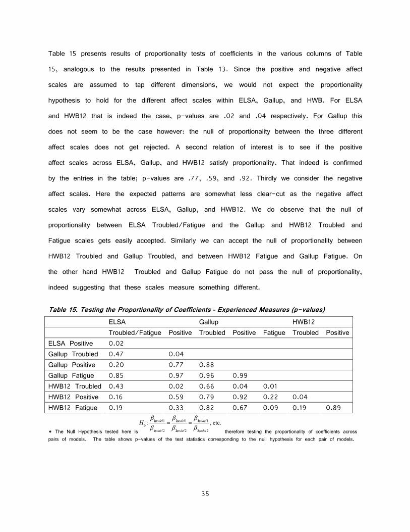
Table 15 presents results of proportionality tests of coefficients in the various columns of Table
15, analogous to the results presented in Table 13. Since the positive and negative affect
scales are assumed to tap different dimensions, we would not expect the proportionality
hypothesis to hold for the different affect scales within ELSA, Gallup, and HWB. For ELSA
and HWB12 that is indeed the case, p-values are .02 and .04 respectively. For Gallup this
does not seem to be the case however: the null of proportionality between the three different
affect scales does not get rejected. A second relation of interest is to see if the positive
affect scales across ELSA, Gallup, and HWB12 satisfy proportionality. That indeed is confirmed
by the entries in the table; p-values are .77, .59, and .92. Thirdly we consider the negative
affect scales. Here the expected patterns are somewhat less clear-cut as the negative affect
scales vary somewhat across ELSA, Gallup, and HWB12. We do observe that the null of
proportionality between ELSA Troubled/Fatigue and the Gallup and HWB12 Troubled and
Fatigue scales gets easily accepted. Similarly we can accept the null of proportionality between
HWB12 Troubled and Gallup Troubled, and between HWB12 Fatigue and Gallup Fatigue. On
the other hand HWB12 Troubled and Gallup Fatigue do not pass the null of proportionality,
indeed suggesting that these scales measure something different.
Table 15. Testing the Proportionality of Coefficients – Experienced Measures (p-values) ELSA Gallup HWB12
* The Null Hypothesis tested here is therefore testing the proportionality of coefficients across pairs of models. The table shows p-values of the test statistics corresponding to the null hypothesis for each pair of models.
H0
:
1,model1
1,model2
2,model1
2,model2
3,model1
3,model2
, etc.
36
7. Conclusions
It is increasingly understood that traditional economic measures are necessary, but not
sufficient, to measure societal progress (Stiglitz et. al, 2009). Accordingly, in recent
decades, research interest has been rising to find broader measures of well-being to be used
to monitor societal progress and evaluate policy. The literature thus far has conceptualized
subjective well-being either as the evaluation of life satisfaction/dissatisfaction (evaluative well-
being measures) or as the combination of experienced affect (range of emotions from joy to
misery).
In this paper, we conducted an experiment to investigate the relations between a number of
evaluative and experienced measures (and one eudemonic measure), using the American Life
Panel (ALP). This is the first time that all these different types of measures have been
collected jointly in a population survey. Although the concepts asked in the different
experienced measures included in our experiment are in some cases the same, measures
differ in the scales of their questions and so, we also studied the correspondence across
these different scales. The experiment confirms a number of findings in the literature and
yields some new results.
Several different evaluative well-being measures are being studied, with two implications in
terms of policy recommendations.
First, we can compare the scales for the single-item life satisfaction items. These were asked
through the SWLS ("I am satisfied with my life", scale 1 to 5, “Strongly disagree” to
“Strongly agree”), SHARE ("How satisfied are you with your life in general?", scale 1 to
4, from “Very satisfied” to “Very dissatisfied”), Gallup ("On which step of the ladder would
you say you stand now?", scale 1 through 10) and ONS ("Overall, how satisfied are you
with your life nowadays?", scale 0 to 10, from “Not at all” to “Completely”). The
correlations between each of those measures are quite high (see Tables 2, 3 and 4); while
the test-retest characteristics are also very comparable, ranging from 0.67 (SHARE) to 0.74
37
(ONS), see Table 5. All four measures also load on the same factor, and we cannot reject
the hypothesis of proportionally of the coefficients on demographic and socio-economic
characteristics (table 13). Thus, we conclude that despite the differences in scales used, the
results are consistent across the different life satisfaction measures.
Second, while we find that all evaluative measures load on the same factor, there are
differences between multi-item and single-item evaluative well-being measures. In particular,
the three single-item questions (SHARE, ONS and Gallup) perform differently than the Diener
scale, whether used as a factor or an average. Given the difference in wording and concepts
elicited by the 5 items, in particular those other than "I am satisfied with my life", this
finding is not surprising. Diener et al. (1985) proposed the use of their five-item scale to
elicitate individuals’ overall judgment of their life, while avoiding the issue of single-item scales
that may be more affected by the particular wording of the question, and that do not provide
an assessment of the separate components of evaluative well-being (Larson, Diener and
Emmons, 1985). While the latter argument is by construction true, our findings show that the
coefficients of demographic and socio-economic characteristics for the single-item scales are,
despite varying scales discussed above, proportional, and thus very comparable. Therefore, if
policy makers are interested in measuring evaluative well-being as a respondent's satisfaction
with his current life, then single-item scales should be used. As shown in table 1, the
response time for single item scales is lower than for multi-item scales, which is of
importance when including new measures in surveys. The use of a multi-item scale as an
aggregated measure of evaluative well-being, such as the Diener scale, is less advisable,
since its results are not aligned with those from single-item measures, and are less
transparent in the concept being measured. If however other dimensions of evaluative well-
being, in particular regarding different time frames, such as satisfaction with the past ("If I
could live my life over, I would change almost nothing"), or expectations about the future
(such as the Cantril Ladder in 5 years as asked by Gallup), are of interest, then the
inclusion of such items would be appropriate. Here again, their inclusion as separate items
38
rather than as an aggregate scale may be more helpful in identifying the concepts being
measured.
Turning to experienced measures of well-being, the positive and negative experienced affect
measures load on different factors, thus confirming that positive and negative affect are not
simply opposite poles on the same scale. Depending on the scale used, we find that negative
affect can be represented by one or two factors. The ONS-happy measure loads both on the
evaluative factor and on both the positive and negative affect factor. It is not entirely clear
why this happens, but one possibility is the design of the ONS questionnaire, which places
this experienced measure directly behind an evaluative question. Both previous points suggest
the need for more work on the structure of questionnaires (response scales, lay-out, question
order, etc.), and that subjective well-being is multidimensional.
The paper pays a fair bit of attention to the effect of scales used for the affect measures.
The different scales imply a different number of underlying factors and different relations with
demographics. This is clearly undesirable given that they all are based on the same items:
The relation between experienced well-being and personal circumstances and demographics
should not depend on whether we use a binary scale, a five-point scale, or a seven-point
scale. In a number of ways the ELSA seven-point scale appears to behave better than the
other coarser scales (especially the Gallup scales). This result confirms the theory of higher
data quality, through higher validity and lower residual error, when using a higher number of
answer categories (Andrews, 1984). Partly this can be ascribed to the fact that with finer
scales, respondents can express their feelings in a more nuanced way, while assumptions of
underlying normal distributions (which motivate many of the statistical procedures) will be
closer to being satisfied by the data.
The relation of evaluative and experienced measures with demographics is markedly different.
For instance, evaluative well-being increases monotonically and almost linearly with income; for
experienced well-being no such relation with income is found. Evaluative well-being shows a
39
U-shaped relation with age, while for experienced well-being no such relation is found. Also,
health and labor market status, which have clear and significant effects on evaluative well-
being, do not appear to have much of a consistent influence on experienced well-being.
Whether one finds a relation or not appears to depend on the kind of response scale used in
eliciting items. In general terms however, it appears that the relation between experienced
measures and demographics is much weaker than between evaluative measures and
demographics.
This finding suggests that evaluative well-being measures may be more relevant for policy
makers, as they allow for a general monitoring of a population. Both experienced and
evaluative measures can be of interest in terms of informing policies, so that ultimately the
choice of measure requires knowing what the measure will be used for as they provide
important information on different dimensions of subjective well-being. The relationship between
life circumstances and evaluative measures is however much stronger and reflects long lasting
factors that could be influenced by policies.
40
References
Alesina, A., Di Tella, R., & MacCulloch, R. (2004). Inequality and happiness: are Europeans and Americans different? Journal of Public Economics, 88(9), 2009-2042.
Alfonso, V. C., Allison, D. B., Rader, D. E., Gorman B. S. (1996). The Extended Satisfaction with Life Scale: Development and Psychometric Properties. Social Indicators Research, 38(3), 275-301.
Andrews, F. M. (1984). Construct validity and error components of survey measures: A structural modeling approach. Public opinion quarterly, 48(2), 409-442.
Blanchflower, D. G., & Oswald, A. J. (2004). Well-being over time in Britain and the USA. Journal of public economics, 88(7), 1359-1386.
Bollen, Kenneth A. (1989) Structural Equation Models with Latent Variables. John Wiley & Sons, Ltd.
Bruine de Bruin, W., VanderKlaauw, W., Downs, J. S., Fischhoff, B., Topa, G., & Armantier, O. (2010). Expectations of inflation: The role of demographic variables, expectation formation, and financial literacy. Journal of Consumer Affairs, 44(2), 381-402.
Campbell, A., Converse, P. E., & Rodgers, W. L. (1976). The quality of American life: Perceptions, evaluations, and satisfactions (Vol. 3508). Russell Sage Foundation.
Cantril, H. (1965). The Pattern of Human Concerns. New Brunswick, NJ, Rutgers U. P.
Clark, A., & Oswald, A. (1994). Unhappiness and Unemployment. The Economic Journal, 104(424), pp 648-659.
Csikszentmihalyi, M., & Hunter, J. (2003). Happiness in everyday life: The uses of experience sampling. Journal of Happiness Studies, 4(2), 185-199.
Deaton, A. (2008). Income, Health, and Well-Being Around the World: Evidence From the Gallup World Poll. Journal of Economic Perspectives, 22(2), 53-72.
Deaton, A. & Stone, A. (2013). Evaluative and hedonic well-being among those with and without children at home. Mimeo.
Delavande, A., & Rohwedder, S. (2008). Eliciting subjective probabilities in Internet surveys. Public Opinion Quarterly, 72(5), 866-891.
Diener, E., Oishi, S., & Lucas, R.E. (2011). The Science of Happiness and Life Satisfaction. In C. R. Snyder & S. J. Lopez (Eds.), The handbook of positive psychology (pp. 63–73). Oxford, England: Oxford University Press.
41
Diener, E. (2000). Subjective well-being: The science of happiness and a proposal for a national index. American psychologist, 55(1), 34.
Diener, E., Emmons, R. A., Larsen, R. J., & Griffin, S. (1985). The satisfaction with life scale. Journal of personality assessment, 49(1), 71-75.
Diener, E., Suh, E.M., Lucas, R.E., and Smith, H. L. (1999). Subjective Well-Being: Three Decades of Progress. Psychological Bulletin, 125(2), pp 276-302.
DiTella, R., MacCulloch, R., Oswald, A.J. (2001). Preferences over inflation and unemployement: evidence from surveys of happiness. American Economic Review, 91, pp 335-341.
Dolan, P., Layard, R., & Metcalfe, R. (2011). Measuring subjective well-being for public policy.
Dolan, P., Peasgood, T., & White, M. (2008). Do we really know what makes us happy? A review of the economic literature on the factors associated with subjective well-being. Journal of Economic Psychology, 29(1), 94-122.
Easterlin, R. (1974). Does Economic Growth Improve the Human Lot? Some Empirical Evidence. In P. A. David & M. W. Reder (Eds.), Nations and Households in Economic Growth: Academic Press.
Easterlin, R. A. (1995). Will raising the incomes of all increase the happiness of all? Journal of Economic Behavior & Organization, 27(1), 35-47.
Eid, M., & Diener, E. (2004). Global judgments of subjective well-being: Situational variability and long-term stability. Social indicators research, 65(3), 245-277.
Fonseca, R., Mullen, K. J., Zamarro, G., & Zissimopoulos, J. (2012). What explains the gender gap in financial literacy? The role of household decision making. Journal of Consumer Affairs, 46(1), 90-106.
Frey, B. S., & Stutzer, A. (2005). Happiness research: State and prospects. Review of social economy, 63(2), 207-228.
Haring, M.J., Okun, M.A., & Stock., W.A. (1984). A quantitative synthesis of literature on work status and subjective well-being. Human Relations, 37, 645-657.
Headey, B., Kelley, J., & Wearing, A. (1993). Dimensions of mental health: life satisfaction, positive affect, anxiety and depression. Social Indicators Research, 29(1), 63-82.
Helliwell, J. F. (2003). How's life? Combining individual and national variables to explain subjective well-being. Economic Modelling, 20(2), 331-360.
Kahneman, D., & Deaton, A. (2010). High income improves evaluation of life but not emotional well-being. Proceedings of the National Academy of Sciences, 107(38), 16489-16493.
42
Kahneman, D., & Krueger, A. B. (2006). Developments in the measurement of subjective well-being. The journal of economic perspectives, 20(1), 3-24.
Kahneman, D., Krueger, A. B., Schkade, D., Schwarz, N., & Stone, A. (2004). Toward national well-being accounts. The American Economic Review, 94(2), 429-434.
Kahneman, D., Krueger, A. B., Schkade, D., Schwarz, N., & Stone, A. A. (2006). Would you be happier if you were richer? A focusing illusion. Science, 312(5782), 1908-1910.
Kahneman, D., Krueger, A. B., Schkade, D. A., Schwarz, N., & Stone, A. A. (2004b). A survey method for characterizing daily life experience: The day reconstruction method. Science, 306(5702), 1776-1780.
Kahneman, D., & Riis, J. (2005). Living, and thinking about it: two perspectives on life. The Science of Well-Being, 285-304.
Kapteyn, A., Smith, J. P., & Van Soest, A. (2010). Life satisfaction. International differences in well-being, pp 70-104.
Kim, J. E., & Moen, P. (2002). Retirement Transitions, Gender, and Psychological Well-Being: A Life-Course, Ecological Model. Journal of Gerontology, 57(3), pp 212-222.
Krueger, A. B., & Schkade, D. A. (2008). The reliability of subjective well-being measures. Journal of Public Economics, 92(8), 1833-1845.
Larsen, R. J., Diener, E. D., & Emmons, R. A. (1985). An evaluation of subjective well-being measures. Social Indicators Research, 17(1), 1-17.
Louis, V. V. & Zhao, S. (2002). Effects of Family Structure, Family SES, and Adulthood Experiences on Life Satisfaction. Journal of Family Issues, 23, pp 986-1005.
Lord, F.M. & Novick, M.R. (1968), Statistical Theories of Mental Test Scores. Reading, Massachusetts: Addison-Wesley.
Lucas, R.E. (2007). Adaptation and the Set-Point Model of Subjective Well-Being: Does Happiness Change After Major Life Events? Current Directions in Psychological Science, 16(2), pp 75-79.
Lucas, R. E., & Lawless, N. M. (2013). Does life seem better on a sunny day? Examining the association between daily weather conditions and life satisfaction judgments. Journal of personality and social psychology, 104(5), 872.
Lusardi, A., & Mitchell, O. S. (2007). Financial literacy and retirement planning: New evidence from the Rand American Life Panel (No. 2007/33). CFS Working Paper.
43
Manski, C. F., & Molinari, F. (2010). Rounding probabilistic expectations in surveys. Journal of Business and Economic Statistics, 28(2), 219-231.
Morrison, D.F. (1990). Multivariate statistical methods. 3rd edition. McGraw-Hill series in probability and statistics.
Olsson, U. (1979). On the robustness of factor analysis against crude classification of the observations. Multivariate Behavioral Research, 14(4), 485-500.
Rugaber, C. S. (2012). Are you happy? Ben Bernanke wants to know.
Ryff, C. D. (1989). Happiness is everything, or is it? Explorations on the meaning of psychological well-being. Journal of personality and social psychology, 57(6), 1069.
Ryff, C. D., & Keyes, C. L. M. (1995). The structure of psychological well-being revisited. Journal of personality and social psychology, 69(4), 719.
Schimmack, U., & Oishi, S. (2005). The influence of chronically and temporarily accessible information on life satisfaction judgments. Journal of personality and social psychology, 89(3), 395.
Schwarz, N., & Strack, F. (1991). Evaluating one’s life: A judgment model of subjective well-being. Subjective well-being: An interdisciplinary perspective, 21, 27-47.
Smith, J. & Stone, A. (2011). Short survey measure of hedonic wellbeing.
Stevenson, B., & Wolfers, J. (2008). Economic growth and subjective well-being: Reassessing the Easterlin paradox (No. w14282). National Bureau of Economic Research.
Stiglitz, J. E., Sen, A., & Fitoussi, J. P. (2009). Report by the commission on the measurement of economic performance and social progress. Paris: Commission on the Measurement of Economic Performance and Social Progress.
Stutzer, A. (2004). The role of income aspirations in individual happiness. Journal of Economic Behavior & Organization, 54(1), pp 89-109.
Tuccitto, D. E., Giacobbi, P. R., & Leite, W. L. (2010). The internal structure of positive and negative affect: A confirmatory factor analysis of the PANAS. Educational and Psychological Measurement, 70(1), 125-141.
Watson, D., Clark, L. A., & Tellegen, A. (1988). Development and validation of brief measures of positive and negative affect: the PANAS scales. Journal of personality and social psychology, 54(6), 1063.
44
Appendix: Questionnaires
Evaluative questions
The Cantril Ladder - Gallup Well-Being Index Please imagine a ladder with steps numbered from 0 at the bottom to 10 at the top. Suppose we say that the top of the ladder represents the best possible life for you and the bottom of the ladder represents the worst possible life for you. On which step of the ladder would you say you personally feel you stand at this time, assuming that the higher the step the better you feel about your life, and the lower the step the worse you feel about it? Which step comes closest to the way you feel? 1/2/3/4/5/6/7/8/9/10
Please imagine a ladder with steps numbered from 0 at the bottom to 10 at the top. Suppose we say that the top of the ladder represents the best possible life for you and the bottom of the ladder represents the worst possible life for you. On which step of the ladder would you say you stood 5 years ago? 1/2/3/4/5/6/7/8/9/10
Please imagine a ladder with steps numbered from 0 at the bottom to 10 at the top. Suppose we say that the top of the ladder represents the best possible life for you and the bottom of the ladder represents the worst possible life for you. On which step of the ladder would you say you will stand on in the future, say about 5 years from now? 1/2/3/4/5/6/7/8/9/10
Diener’s Satisfaction With Life Scale– HRS/ELSA Please say how much you agree or disagree with the following statements:
In most ways my life is close to ideal. Strongly disagree/ Somewhat disagree/ Slightly disagree/ Neither agree or disagree/ Slightly agree/ Somewhat agree/ Strongly agree The conditions of my life are excellent. Strongly disagree/ Somewhat disagree/ Slightly disagree/ Neither agree or disagree/ Slightly agree/ Somewhat agree/ Strongly agree I am satisfied with my life. Strongly disagree/ Somewhat disagree/ Slightly disagree/ Neither agree or disagree/ Slightly agree/ Somewhat agree/ Strongly agree So far, I have gotten the important things I want in life.
45
Strongly disagree/ Somewhat disagree/ Slightly disagree/ Neither agree or disagree/ Slightly agree/ Somewhat agree/ Strongly agree If I could live my life again, I would change almost nothing. Strongly disagree/ Somewhat disagree/ Slightly disagree/ Neither agree or disagree/ Slightly agree/ Somewhat agree/ Strongly agree
Life satisfaction - SHARE How satisfied are you with your life in general? Very satisfied / Somewhat satisfied / Somewhat dissatisfied/ Very dissatisfied
ONS – ELSA Overall, how satisfied are you with your life nowadays? (Not at all) 0/1/2/3/4/5/6/7/8/9/10 (Completely) Overall, how happy did you feel yesterday? (Not at all) 0/1/2/3/4/5/6/7/8/9/10 (Completely) Overall, how anxious did you feel yesterday? (Not at all) 0/1/2/3/4/5/6/7/8/9/10 (Completely) Overall, to what extent do you feel that the things you do in your life are worthwhile? (Not at all) 0/1/2/3/4/5/6/7/8/9/10 (Completely)
46
Experienced Questions – ELSA
Now, please pause briefly to think about yesterday, from the morning until the end of the
day. Think about where you were, what you were doing, who you were with, and how you
felt.
- What day of the week was it yesterday? - What time did you wake up yesterday? - What time did you go to sleep at the end of the day yesterday? - Yesterday, did you feel any pain? None/ A little/ Some/ Quite a bit/ A lot - Did you feel well-rested yesterday morning (that is, you slept well the night before)?
Yes/ No - Was yesterday a normal day for you or did something unusual happen? Yes, just a
normal day / No, my day included unusual bad (stressful) things/ No, my day included unusual good things
Please think about the things you did yesterday. How did you spend your time and how did you feel?
- Yesterday, did you watch TV? Yes / No (skip next 2 question) o How much time did you spend watching TV yesterday? o How did you feel when you were watching TV yesterday?
Matrix showing: Happy/ Interested/ Frustrated/ Sad
- Yesterday, did you work or volunteer? Yes / No (skip next 2 question) o How much time did you spend working or volunteering yesterday? o How did you feel when you were working or volunteering yesterday?
Matrix showing: Happy/ Interested/ Frustrated/ Sad
- Yesterday, did you go for a walk or exercise? Yes / No (skip next 2 question) o How much time did you spend walking or exercising yesterday? o How did you feel when you were walking or exercising yesterday?
Matrix showing: Happy/ Interested/ Frustrated/ Sad
- Yesterday did you do any health-related activities other than walking or exercise? For example, visiting a doctor, taking medications or doing treatments. Yes / No (skip next 2 question)
o How much time did you spend doing health-related activities yesterday? o How did you feel when you were doing health-related activities yesterday?
Matrix showing: Happy/ Interested/ Frustrated/ Sad
47
- Yesterday did you travel or commute? E.g. by car, train, bus etc. Yes / No (skip next 2 question)
o How much time did spend travelling or commuting yesterday? o How did you feel when you were travelling or commuting yesterday?
Matrix showing: Happy/ Interested/ Frustrated/ Sad
- Yesterday did you spend time with friends or family? Yes / No (skip next 2 question)
o How much time did you spend with friends or family yesterday? o How did you feel when you were with friends or family yesterday?
Matrix showing: Happy/ Interested/ Frustrated/ Sad
- Yesterday did you spend time at home by yourself? Without a spouse, partner or anyone else present. Yes / No (skip next 2 question)
o How much time did you spend at home by yourself yesterday? o How did you feel when you were at home by yourself yesterday?
Matrix showing: Happy/ Interested/ Frustrated/ Sad Additional module:
- Overall, how did you feel yesterday? Rate each feeling on a scale from 0 – did not experience at all – to 6 – the feeling was extremely strong.
- Did you experience anger during a lot of the day yesterday? Yes/No - Did you experience depression during a lot of the day yesterday? Yes/No - Did you experience enjoyment during a lot of the day yesterday? Yes/No - Did you experience happiness during a lot of the day yesterday? Yes/No - Did you experience sadness during a lot of the day yesterday? Yes/No - Did you experience stress during a lot of the day yesterday? Yes/No - Did you experience worry during a lot of the day yesterday? Yes/No
- Now, please think about yesterday, from the morning until the end of the day. Think
about where you were, what you were doing, who you were with, and how you felt. Did you learn or do something interesting yesterday? Yes/No
- Now, please think about yesterday, from the morning until the end of the day. Think about where you were, what you were doing, who you were with, and how you felt. Did you smile or laugh a lot yesterday? Yes/No
- Now, please think about yesterday, from the morning until the end of the day. Think about where you were, what you were doing, who you were with, and how you felt. Were you treated with respect all day yesterday? Yes/No
- Now, please think about yesterday, from the morning until the end of the day. Think about where you were, what you were doing, who you were with, and how you felt. Would you like to have more days just like yesterday? Yes/No
Additional module
- Did you experience enthusiasm during a lot of the day yesterday? Yes/No - Did you experience contentment during a lot of the day yesterday? Yes/No - Did you experience frustration during a lot of the day yesterday? Yes/No - Did you experience fatigue during a lot of the day yesterday? Yes/No - Did you experience loneliness during a lot of the day yesterday? Yes/No - Did you experience boredom during a lot of the day yesterday? Yes/No - Did you experience pain during a lot of the day yesterday? Yes/No
- What time did you wake up yesterday? …..:…… - What time did you go to bed yesterday? …..:…… - Did you feel well-rested yesterday morning (that is, you slept well the night before)?
Yes/No - Was yesterday a normal day for you or did something unusual happen?
o Yes, just a normal day / No, my day included unusual bad (stressful) things/ No, my day included unusual good things
49
Please think about the things you did yesterday. How did you spend your time and how did you feel?
- Yesterday, did you watch TV? Yes / No (skip next question) o How much time did you spend watching TV yesterday?
- Yesterday, did you work or volunteer? Yes / No (skip next question) o How much time did you spend working or volunteering yesterday?
- Yesterday, did you go for a walk or exercise? Yes / No (skip next question) o How much time did you spend walking or exercising yesterday?
- Yesterday did you do any health-related activities other than walking or exercise? For example, visiting a doctor, taking medications or doing treatments. Yes / No (skip next question)
o How much time did you spend doing health-related activities yesterday? - Yesterday did you travel or commute? E.g. by car, train, bus etc. Yes / No (skip
next question) o How much time did spend travelling or commuting yesterday?
- Yesterday did you spend time with friends or family? Yes / No (skip next question) o How much time did you spend with friends or family yesterday?
- Yesterday did you spend time at home by yourself? Without a spouse, partner or anyone else present. Yes / No (skip next question)
o How much time did you spend at home by yourself yesterday? [2 activities reported by the respondent were randomly selected for the ELSA experienced affect module. For example, if activity “walking or exercising was chosen, the question was:]
- How did you feel when you were walking or exercising? Rate each feeling on a scale from 0 – did not experience at all – to 6 – the feeling was extremely strong.
o Matrix showing: Happy/ Interested/ Frustrated/ Sad
50
Experienced Questionnaire – HWB-12
Now we would like you to think about yesterday. What did you do yesterday and how did
you feel?
- To begin, please tell me what time you woke up yesterday: ………….. - And what time did you go to sleep yesterday?…………..
Now please take a few quiet seconds to recall your activities and experiences yesterday Good, now I have questions about your experiences yesterday. [Randomized order of emotions]
- Yesterday, did you feel happy?
o Would you say: Not at all/ A little/ Somewhat/ Quite a bit/ Very - Yesterday, did you feel enthusiastic?
o Would you say: Not at all/ A little/ Somewhat/ Quite a bit/ Very - Yesterday, did you feel content?
o Would you say: Not at all/ A little/ Somewhat/ Quite a bit/ Very - Yesterday, did you feel angry?
o Would you say: Not at all/ A little/ Somewhat/ Quite a bit/ Very - Yesterday, did you feel frustrated?
o Would you say: Not at all/ A little/ Somewhat/ Quite a bit/ Very - Yesterday, did you feel tired?
o Would you say: Not at all/ A little/ Somewhat/ Quite a bit/ Very - Yesterday, did you feel sad?
o Would you say: Not at all/ A little/ Somewhat/ Quite a bit/ Very - Yesterday, did you feel stressed?
o Would you say: Not at all/ A little/ Somewhat/ Quite a bit/ Very - Yesterday, did you feel lonely?
o Would you say: Not at all/ A little/ Somewhat/ Quite a bit/ Very - Yesterday, did you feel worried?
o Would you say: Not at all/ A little/ Somewhat/ Quite a bit/ Very - Yesterday, did you feel bored?
o Would you say: Not at all/ A little/ Somewhat/ Quite a bit/ Very - Yesterday, did you feel pain?
o Would you say: Not at all/ A little/ Somewhat/ Quite a bit/ Very Additional module [Randomized order of emotions]
- Yesterday, did you feel depressed?
51
o Would you say: Not at all/ A little/ Somewhat/ Quite a bit/ Very - Yesterday, did you feel joyful?
o Would you say: Not at all/ A little/ Somewhat/ Quite a bit/ Very - Yesterday, did you learn or do something interesting?
o Would you say: Not at all/ A little/ Somewhat/ Quite a bit/ Very - Did you feel well-rested yesterday morning (that is, you slept well the night before)?
Yes / No - Was yesterday a normal day for you or did something unusual happen?
o Yes, just a normal day / No, my day included unusual bad (stressful) things/ No, my day included unusual good things
Please think about the things you did yesterday. How did you spend your time and how did you feel?
- Yesterday, did you watch TV? Yes / No (skip next question) o How much time did you spend watching TV yesterday?
- Yesterday, did you work or volunteer? Yes / No (skip next question) o How much time did you spend working or volunteering yesterday?
- Yesterday, did you go for a walk or exercise? Yes / No (skip next question) o How much time did you spend walking or exercising yesterday?
- Yesterday did you do any health-related activities other than walking or exercise? For example, visiting a doctor, taking medications or doing treatments. Yes / No (skip next question)
o How much time did you spend doing health-related activities yesterday? - Yesterday did you travel or commute? E.g. by car, train, bus etc. Yes / No (skip
next question) o How much time did spend travelling or commuting yesterday?
- Yesterday did you spend time with friends or family? Yes / No (skip next question)
o How much time did you spend with friends or family yesterday? - Yesterday did you spend time at home by yourself? Without a spouse, partner or
anyone else present. Yes / No (skip next question) o How much time did you spend at home by yourself yesterday?
[2 activities reported by the respondent were randomly selected for the ELSA experienced affect module. For example, if activity “walking or exercising was chosen, the question was:]
- How did you feel when you were walking or exercising? Rate each feeling on a scale from 0 – did not experience at all – to 6 – the feeling was extremely strong.
o Matrix showing: Happy/ Interested/ Frustrated/ Sad
52
The Impact of Employment Transitions on Subjective Well-being: Evidence
from the Great Recession and its Aftermath
Michael Hurd
Susann Rohwedder
Caroline Tassot
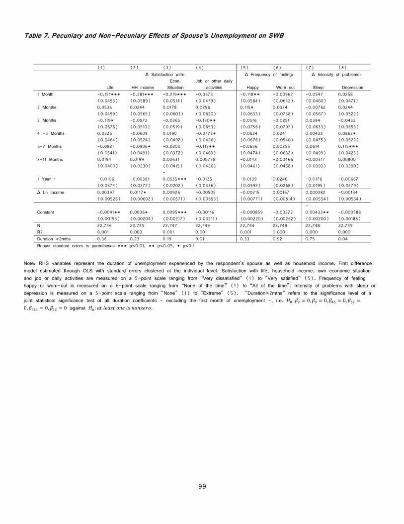
We use 42 waves of the Financial Crisis Surveys collected in the American Life Panel to
estimate the causal effect of work transitions, in particular unemployment and reemployment, on
subjective well-being (SWB) between November 2009 and April 2013 in the US. We find
unemployment to negatively affect evaluative and experienced SWB in the first month of
unemployment, with very little changes in subsequent months, thus indicating a lack of
adaptation. Reemployment leads to significant increases in SWB, with no evidence of
adaptation after the first month. The consequences of work transitions spillover at the
household level, with individuals being affected by their spouses’ work transitions. We find no
evidence of a “scarring” effect of unemployment. Given this lack of adaption to unemployment,
policies supporting the unemployed are necessary. Financial support is crucial, but should also
be complemented with measures targeting the non-pecuniary loss in SWB suffered due to
unemployment, for instance through the provision of a support network or job search
assistance.
53
1. Introduction
There is a large literature that studies the impact of labor force status on subjective well-
being with most contributions coming from the fields of psychology and economics. Labor force
status, and in particular unemployment, is a recurring source of concern for governments in
Western economies. The cost of high rates of unemployment for an economy are tremendous,
extending well beyond the pecuniary cost of economies operating below their potential, as
unemployment also affects people’s lives at the social level (Winkelmann and Winkelmann,
1998).
Empirical analyses have consistently found unemployment to be associated with lower individual
well-being (Clark and Oswald 1994; McKee-Ryan et al., 2005; Clark, Knabe and Rätzel,
2010). For instance, life satisfaction scores were found to be between 5 and 15% lower
among unemployed individuals compared to employed individuals (Dolan, Peasgood and White,
2008).
This effect can be broken down into two major components. First, pecuniary effects reflect the
changes in subjective well-being due to fluctuations in income. Second, non-pecuniary effects
are the result of the reversal of latent functions of employment, such as a sense of self-
esteem or access to a social network, independently of any changes in income.
The pecuniary effect has overwhelmingly been assessed by looking at how a decrease in
income as a result of unemployment impacts subjective well-being. While estimates of the
income loss following employment range from 40% to 50% of pre-unemployment income,
studies estimate this drop in income to represent only about 14% of the total well-being cost
in Germany, and at most 10% in the UK (Winkelmann and Winkelmann, 1998; Clark and
Oswald, 2002).
The non-pecuniary cost of unemployment has been evaluated in numerous studies, typically by
controlling for income when estimating models that have subjective well-being as the
54
dependent variable and unemployment as an independent variable (Dolan, Peasgood and
White, 2008). Using this methodology to study the German Socio-Economic Panel, Lucas et
al. (2004) find a half-point difference in satisfaction on a ten-point scale after individuals
became unemployed. Based on the British Household Panel Study, Clark and Oswald (2002)
and Wildman and Jones (2002) report an average loss in subjective well-being due to
unemployment of 1.3 and 1.65 points respectively on a 36 point-scale, while Winkelmann
(2006) finds a 0.85 point loss on a 0-10 scale in Germany.
The role played by the duration of unemployment spells on subjective well-being is particularly
interesting. From a theoretical point of view, the ‘hedonic treadmill’ model and set-point theory
in psychology predict that while individuals’ happiness might be temporarily affected by events,
they could actually adjust to their new circumstances and thereby adapt back to `hedonic
neutrality’ – that is, their pre-event initial levels of happiness (Diener, Lucas and Scollon,
2006). However, as pointed out by Lucas et al. (2004), testing the set-point theory
requires longitudinal data that would allow for the observation of subjective well-being levels
during the months or years leading up to an event. One such longitudinal study found
indications of adaptation, while tracking the subjective well-being levels of 115 recent college
graduates (Suh, Diener and Fujita, 1996). Subjective well-being was shown to fluctuate in
response to a range of life events the study subjects experienced, and then return to prior
levels with time. Whether there is empirical support for the set-point theory is unclear. There
is for instance a debate around the evidence of adaptation to marital transitions, with some
claiming evidence supporting a quick and complete return to pre-marriage levels (see for
example Lucas et al., 2003; Lucas and Clark, 2006) – thus supporting the set-point
theory-, and others finding a lasting effect of marriage (Easterlin, 2003; Zimmermann and
Easterlin, 2006). A similar debate revolves around the adaptation to health events (see
Easterlin, 2003).
In regards to the event of unemployment, the evidence of such adaptation is mixed. On the
one hand, for Clark and Oswald (1994) find evidence of adaptation when comparing
55
members of the British Household Panel Study who had been employed for less than six
months with other members who had been out of work for at least two years. Their finding
was that, as an unemployment spell lengthens, its adverse effect on subjective well-being
weakens. On the other hand, German data from the GSOEP does not support the adaptation
theory. Winkelmann and Winkelmann (1998) find an insignificant coefficient of unemployment
duration on life satisfaction in a model including individual fixed effects. Clark et al. (2008)
and Clark and Georgellis (2012) show a long lasting effect of lower life satisfaction several
years after the onset of unemployment, again using the GSOEP and BHPS. However, they
also observe a positive interaction between past and current unemployment, meaning that
someone newly unemployed who has experienced unemployment in the past will experience
less negative effects from the current event of unemployment. This process is identified as
“habituation.”
In another study, using weekly surveys of individuals receiving unemployment insurance in New
Jersey between 2009 and 2010, Krueger and Mueller (2011) find little change in life
satisfaction over the course of an unemployment spell, though they do find an increase in
self-reported bad mood and a decrease in self-reported good mood. While their weekly data
provides a unique high-frequency picture of possible adaptation, the restriction of the sample
to unemployed individuals receiving unemployment benefits is challenging. For instance, it does
not permit the study of the effect of transitions in work status, since throughout the survey
respondents are consistently unemployed. Instead, the responses of the unemployed in New
Jersey in 2009 are compared to nationwide data collected in 2006 from a sample of the
employed in the Princeton Affect and Time-Use Survey. Another limitation is the assumption
that adaptation is linear in the duration of unemployment. A further constraint of this study is
that only the receipt of unemployment benefits is taken into account, with no consideration for
any other sources of income. Thus the evidence in the US in terms of adaptation is limited,
since only the effect of experiencing unemployment for at least one month in the past 10
years (Louis and Zhao, 2002), and the time path of subjective well-being following
56
unemployment for up to 24 weeks in New Jersey (Krueger and Mueller, 2011) have been
examined.
While one would expect the pecuniary effects of unemployment to be shared in the household,
it is less obvious whether the same would apply to the non-pecuniary effects. The non-
pecuniary effects for other household members could arise in several ways. For example,
they could be due to altered behaviors of the unemployed person towards other household
members or due to other household members’ responses to observing the change in
satisfaction and happiness of the unemployed person. Such externalities can for example put
children of unemployed fathers at increased risk for deviant behavior and lower aspirations and
expectations (Clark, Knabe and Rätzel, 2010). Unemployment can also significantly affect
spouses, who are faced with their partner’s lower well-being and increased presence in the
household (Winkelmann and Winkelmann, 1995; Frey and Stutzer, 2002, Kim and Do,
2013); though this effect can interestingly be attenuated if the spouse becomes unemployed
as well (Clark, 2003).
The number of studies dedicated to studying the effects of unemployment on subjective well-
being stands in sharp contrast to the number of studies focusing on the effect of
reemployment. One of the few studies is that by Lucas and al. (2004) which uses data
from the German Socio-Economic Panel (GSOEP). The authors find an increase in life
satisfaction, but do not find evidence of a return to pre-unemployment levels of well-being
after unemployment spells end. Rather, they conclude that unemployment spells decrease the
set-point for life satisfaction. Others have also found past unemployment to be associated with
lower subjective well-being for those who are currently employed using the same panel (Clark
et al., 2008; Clark, Georgellis and Sanfey, 2001). Turning to the US, data from the
General Social Survey from 1989 to 1994 show that individuals who have been consistently
employed in the past 10 years have higher well-being scores than those who had been
through unemployment spells (Louis and Zhao, 2002). These findings point towards a
“scarring” of individuals who experience unemployment. The thesis behind that notion is that
57
an individual’s satisfaction level will be lower, even if reemployed, according to the number of
months or years spent out of work during their lifetime. This in turn could be due to the
characteristics of subsequent jobs, which could be of lower quality, or provide less job
security.
Overall, there is a broad range of empirical evidence that documents the importance of
individuals’ employment status for their own and others’ subjective well-being. Nonetheless, the
studies so far are subject to several limitations. One example are the constraints presented by
the data. For instance data may only be cross-sectional (Clark and Oswald, 1994), the
panels based on a low-frequency (yearly) (Winkelmann and Winkelmann, 1998; Clark,
2003; Kim and Do, 2013), and the sample restricted (Krueger and Mueller, 2011). Another
issue is that these studies may not take into account intra-household dynamics. What is
more, mostly they focus on a single subjective well-being outcome, such as satisfaction with
life in general. Finally, they are mainly based on European data.
Therefore the contribution of our paper is four-fold. First, the high-frequency data allow us to
observe on a monthly basis the employment status, subjective well-being, and income of
respondents. Thus we are able to closely track evolutions that otherwise might be lost in data
collected yearly. Second, the panel nature of the data allows us to draw causal inference on
the impact of unemployment spells as we can control for fixed effects by estimating a first-
difference model. Third, we investigate the effect of unemployment on multiple dimensions of
subjective well-being over and beyond those related to general life satisfaction, including
experienced subjective well-being measures such as issues with sleep or depression. Fourth,
we study spill-over effects of spousal unemployment on an individual’s subjective well-being.
We examine an individual’s change in subjective well-being in response to the spouse’s
unemployment and compare the response to that observed in response to an individual’s own
unemployment.
58
The policy implications of this work focus on identifying the consequences of unemployment,
both at the individual and the household level on subjective well-being. Understanding the
evolution of subjective well-being over the course of a transition into unemployment and during
an unemployment spell helps identify those who suffer the most. For instance, studying the
potentially different effects of unemployment between the short-term and the long-term
unemployed, and in particular understanding whether individuals adapt to their work situation
helps define intervention opportunities for policies. We thus provide evidence, for the United
States, on pecuniary and non-pecuniary effects of employment transitions on subjective well-
being, as well as on potential adaptation to a new work status.
In this study we use panel data from the RAND American Life Panel Financial Crisis Surveys,
a unique high-frequency longitudinal dataset to estimate the causal effects of income shocks
induced by employment transitions in the wake of the Financial Crisis on subjective well-being.
The remainder of the paper is structured as follows. The next section describes the data,
including the analytical sample and survey items that are central to our analysis. Section 3
provides descriptive statistics for labor market transitions observed in our sample and the
various measures of subjective well-being. Section 4 presents the empirical strategy
implemented to answer the above-mentioned research questions. Section 5 presents results,
first regarding the effects of unemployment on subjective well-being, then in the case of
reemployment and subjective well-being. Section 6 discusses those results, while Section 7
concludes.
2. Data
We use 42 waves of panel data from the American Life Panel Financial Crisis Surveys. The
latter were collected in the RAND American Life Panel to track the experience of American
households during the Great Recession and its aftermath. They were initiated, designed, and
fielded by Susann Rohwedder and Michael Hurd7. The first wave was collected in November
7 Rohwedder and Hurd obtained funding for the ALP Financial Crisis Surveys through various grants from the National Institute on Aging and from the Social Security Administration.
59
2008, and the second in February/March of 2009. Between May 2009 and April 2013 the
ALP Financial Crisis Surveys were conducted every month. Every third interview was longer
than the intervening other monthly interviews to accommodate the collection of additional
information every quarter. Since April 2013 the ALP Financial Crisis Surveys have been
fielded every quarter. Our sample covers the period from November 2009 to April 2013. This
period covers the rise of the unemployment rate associated with the Great Recession and the
years with the highest unemployment rates observed since the early 1980s. At the beginning
of the observation period, the sample had about 2,500 respondents, with response rates
averaging close to 80% (Hurd and Rohwedder, 2010). Refresher samples were added in
November 2011 and in October and November of 2012. The current sample has about
4,000 respondents, with response rates averaging 78% (see Table A1 in the Appendix).
The data are collected over the Internet; respondents who do not have access to the Internet
are provided a Web TV or a laptop, including an Internet access subscription and an e-mail
account. Accordingly the sample does not suffer from selection due to a lack of Internet
access. The surveys cover a broad range of topics, including various dimensions of life
satisfaction, self-reported health measures and indicators of affect, labor force status, recent
job loss and chances of future job loss, as well as various measures of wealth and income.
The subjective well-being measures of interest in this study cover various dimensions of
subjective well-being, and include both evaluative and experienced measures.
In particular, we use the following measures, which have been collected on a monthly basis:
Question Answer options Taking all things together, how satisfied are you with your life as a whole these days? Very satisfied, Satisfied, Neither
satisfied nor dissatisfied, Dissatisfied, Very dissatisfied
How satisfied are you with the total income of your household? How satisfied are you with your overall economic situation? How satisfied are you with your job or other daily activities? During the past 30 days, how much of the time have you felt worn out? All of the time, Most of the
time, A good bit of the time, Some of the time, A little of the time, None of the time
During the past 30 days, how much of the time have you been a happy person?
Overall in the last 30 days, how much difficulty did you have sleeping, such as falling asleep, waking up frequently during the night or waking up too early in the
None, Some, Moderate, Severe, Extreme
60
morning? Overall in the last 30 days, how much of a problem did you have with feeling sad, low, or depressed? Note: emphasis in bold as shown in the surveys.
Overall life satisfaction, as well as satisfaction with particular domains such as total household
income, the overall economic situation or one’s job or daily activities are categorized as
evaluative well-being measures. The latter involve the elicitation of the respondent’s
assessment of his or her situation through a retrospective judgment. In contrast, items referring
to the frequency of feeling happy or worn out, as well as the intensity of sleep or depression
problems represent experienced well-being measures. Those measures focus on the
respondent’s emotional state for a defined reference period (see Kapteyn et al, 2013 for a
review of categories of subjective well-being).
Information about respondents’ household income received “last calendar month” is also
queried every month. For our analysis we construct total household income as the sum of the
respondent’s earnings, his/her spouse’s earnings – if any -, plus “any other income” such
as “income from investments such as dividends, interest or rental income”; “retirement income
such as Social Security, pensions or other annuities”; and “government benefits such as
unemployment, disability, Social Security benefits, or other welfare benefits”.
We restrict the analytical sample to individuals younger than 70 years old, living in stable
households, that is, without any changes in the number of household members and with a
constant marital status between any two consecutive months. These sample restrictions aim at
eliminating potentially confounding factors associated with changes in the household structure
that could affect the estimated parameters of interest. The analysis focuses on respondents in
their working years, for whom unemployment is a meaningful concept. The effect of
unemployment on subjective well-being may be confounded by the effect of a spouse being
unemployed simultaneously. We thus exclude person-waves in which both the respondent and
his/her spouse experienced unemployment spells at the same time. This eliminates 259
person-waves pertaining to 95 respondents. The analytical sample is further limited to
61
individuals for whom the employment status is observed and accounted for in the count of
durations, whether during employment or unemployment. Our analytical sample for this study
has a total of 37,081 person-wave observations, pertaining to 2,456 individuals. The details
of the sample selection are presented in the Table A2 in the Appendix.
3. Descriptive statistics
Table 1 displays the distribution of observed employment transitions for respondents and their
spouses from one month to the next, pooling all 42 waves. Respondents were allowed to
indicate multiple options for their work status in the survey. We excluded person-wave
observations where the respondent indicated self-employment in addition to working for pay or
being unemployed, because income and unemployment among self-employed is difficult to
interpret. We applied the same restrictions for the spouse’s employment transitions. The
majority of person-wave transitions do not involve a change, whether occurring from
employment to employment (92% of respondents, 94% of spouses), or from unemployment to
unemployment (5.5% of respondents, 3.5% of spouses). About 1.3% of person-wave
transitions for the respondent and 1% for the spouses however represent changes from
unemployment to employment and vice-versa.
Figure 1 shows the distribution of evaluative measures, such as satisfaction with “life as a
whole” and other domains of satisfaction, measured on a 5-point Likert scale ranging from
“Very satisfied” to “Very dissatisfied.” The distribution in our sample resembles that of a very
similar item in the Panel Study of Income Dynamics for the period 2007-2009 (see for
example Huang, 2012). On average, our sample shows the lowest satisfaction with regards
to the respondents’ economic situation (3.0), and the highest when they are rating their life
in general (3.7).
Figure 2 shows the distribution of evaluative measures for the frequency respondents reported
having “felt worn out” and having “been happy” in the last 30 days, on a 6-point scale
(from “All of the time” to “None of the time”). More than half of the sample reported
62
being happy “most of the time” while around 41% reported feeling worn-out “a little of the
time”. Finally, figure 3 shows the distribution of depression problems and difficulties sleeping
on a 5-point scale (from “None” to “Extreme”). About half the respondents report having
some problems with sleep or depression.
Figure 4 displays the average of the changes in respondents’ subjective well-being between
month t-1 and t by employment transition. Respondents whose employment status does not
change from one month to the next do not experience any changes in subjective well-being
on average, irrespective of the measure of subjective well-being and irrespective of whether
they are employed or unemployed. Respondents transitioning from employment to
unemployment experience losses in satisfaction with life, household income, their economic
situation, as well as with their job or daily activities. They also feel less happy, experience
more difficulties sleeping and report more severe depression problems. The opposite transition,
from unemployed to employed, appears to trigger the opposite effect, with higher evaluative
well-being, increased happiness, fewer difficulties sleeping, and fewer depression symptoms on
average. The differences in the reported frequency of feeling worn-out seem to reflect a
reduction of fatigue when becoming unemployed, and an increase when finding employment
again.
Figure 5 displays the average of the changes in respondents’ subjective well-being between
month t-1 and t by the employment transition of his or her spouse. About two-thirds of the
person-wave observations (65.1%, N=24,126) in the sample pertain to married persons or
those in a marriage-like relationship (planning their financial future together). The changes in
respondents’ subjective well-being in response to the spouse becoming unemployed are
qualitatively similar to those displayed in figure 4, with respondents whose spouses transitioned
from employment to unemployment experiencing losses in satisfaction with life, household
income, with their economic situation, as well as with their job or daily activities. They also
feel less happy, experience more difficulties sleeping and report more severe depression. The
re-employment of a spouse following his or her unemployment leads to higher evaluative well-
63
being, and less depression. In contrast with figure 4, the differences in feeling worn-out seem
to reflect a slight increase in fatigue when a spouse becomes unemployed, and a reduction in
fatigue when one’s spouse finds a job.
The panel nature of our data allows us to control for individual fixed effects, so that the
effect of an onset of unemployment and reemployment on subjective well-being displayed in
Figures 4 and 5 can be interpreted as causal without any further assumptions. The
subsequent analysis confirms those findings, and further allows us to study the time path of
subjective well-being by distinguishing varying durations of unemployment and re-employment.
The regression framework also permits the inclusion of changes in income as an explanatory
variable, and therefore to draw causal conclusions as to the pecuniary and non-pecuniary
effects.
4. Empirical strategy
To estimate the causal effect of unemployment on SWB and its time trajectory as
unemployment persists we use a first-difference model.
To identify the total effect of unemployment on subjective well-being as a function of
unemployment duration, consider the following model:
∆ 1 2 ⋯ ∆ (1)
Where the Month1 through variables represent indicators of whether the individual i
reached a certain unemployment spell length (measured in months) at the time � is
measured. By construction, individuals who remained employed throughout the past and current
month and thus have a zero length of unemployment will serve as the control group. The
left-hand side variables, represented by , are the subjective well-being items described
above, i.e. life satisfaction, satisfaction with total household income, the economic situation and
one’s job or daily activities, as well as the frequency of feeling worn-out or happy, and the
intensity of problems with sleep and depression. We regressed the change in those subjective
well-being items between month t and month t-1 on indicators for the duration of the
64
unemployment spell, using ordinary least squares (OLS), adjusting the standard errors for the
fact that each respondent contributes multiple observations.
This model specification allows for non-linear effects of unemployment duration on individual
subjective well-being through the inclusion of duration indicators rather than a continuous
duration variable. In order to assess the differences in the total effects of unemployment for
individuals who are married (or in marriage-like relationships and planning their financial future
together) and those who are single, we estimated this model separately for the married and
singles samples.
In order to distinguish between the pecuniary and non-pecuniary effects of unemployment, we
extended the model above to include changes in household income as an explanatory variable:
∆ 1 2 ⋯ ∆ ∆ (2)
The variable Income represents the log value of total monthly household income. The
coefficient identifies the pecuniary impact of unemployment on subjective well-being. The
non-pecuniary costs of own unemployment are identified by the indicators of unemployment
spell length, the β coefficients, which also show the estimated time trajectory of subjective
well-being. For instance, the coefficient indicates the effect of a respondent starting an
unemployment spell and thus being in his or her first month of unemployment rather than
staying employed. The coefficient then shows the effect of transitioning from his first month
of unemployment into his second month of unemployment. not being not statistically
significant would then suggest a lack of change when entering the second month of
unemployment, whereas if is negative (positive) it would indicate a decrease (increase)
in subjective well-being between the first and second month of unemployment. Like the
previous model, we also estimated this model separately for single and married persons.
To investigate how an individual’s own subjective well-being is affected when the
unemployment is experienced by the spouse rather than the individual him or herself, the logic
65
will be similar, now including unemployment variables related to the spouse’s unemployment
duration:
∆ 1 2 ⋯ ∆ (3)
Where the 1 through variables represent indicators of whether individual i’s
spouse s has reached a certain length of unemployment spell measured in months. Finally, in
order to disentangle the pecuniary and non-pecuniary effects of unemployment in this
framework, we added the difference in log household income:
∆ 1 2 ⋯ ∆ ∆ (4)
Comparing estimates from models (1) and (3), and in particular the difference between the
coefficients on spouse ( ) and respondent ( ) unemployment spell duration
indicators allows us to measure the differences in the impact of unemployment depending on
who experiences it in the household. Similarly, comparing the estimates from models (2) and
(4) provides information on the differences in non-pecuniary effects resulting from
unemployment, since household income will be kept constant.
Finally, we study the effect of re-employment on subjective well-being by replicating models
(1) through (4), using indicators for the number of months that have elapsed since a
respondent or his/her spouse got reemployed. Because the effect of re-employment could
plausibly vary depending on how long someone had been unemployed prior to re-employment
we added to the model an interaction between the length of unemployment experienced prior
to the reemployment spell and the onset of reemployment. Individuals or spouses with
continuous unemployment throughout the past and current month serve as the control group in
this estimation.
66
5. Results
The Effect of Unemployment
This section presents the results of models (1) through (4), using as explanatory variables
the duration of unemployment following a transition from employment to unemployment as well
as the log of total household income. The unemployment duration is included through a set of
indicator variables reflecting a period of one month, two months, three months, four to five
months, six to seven months, eight to eleven months, one year or more.
Own Unemployment and Subjective Well-Being: Overall Effects
The coefficient estimates for model (1) for single individuals are displayed in Table 2. The
various subjective well-being indicators are specified in the top row of the table. Each column
represents the estimates of the effects of the explanatory variables on the subjective well-
being measure listed in the top-row. Columns 1 through 4 report the results of the model,
when specified with evaluative subjective well-being measures. Columns 5 and 6 display the
results when explaining the frequency of feeling happy or worn out in the past 30 days.
Finally, columns 7 and 8 display the results with the intensity of sleep and depression
problems as left-hand side variables. Figure 6 provides a visual display of the coefficients for
the evaluative well-being measures, as well as of their 95% confidence intervals, while Figure
7 displays those estimates for experienced well-being items. Thus, estimates with confidence
intervals crossing the 0-line are not statistically significant at the 5% significance level.
According to our estimates single individuals experience a statistically significant deterioration in
all subjective well-being measures at the time when they become unemployed (duration of
unemployment of one month), with just one exception. The coefficient for the first month of
unemployment in column (6) suggests that there is a reduction in “feeling worn out” –
which would seem to be an improvement at least in this dimension – but this effect is not
statistically significant. In terms of magnitudes, the evaluative satisfaction measures are all
elicited using a 5-point scale and the point estimates of the reductions in subjective well-
67
being at the onset of unemployment are -0.21 for satisfaction with life, -.29 for satisfaction
with household income, -0.32 for satisfaction with one’s own economic situation and -0.47
for satisfaction with job or daily activities (-0.47). The frequency of reporting to be happy
in the last 30 days (Table 2, column 5) is also reduced (-0.12 on a 6-point scale) at
the onset of unemployment for single individuals in comparison to those who remained
employed, but barely statistically significant. Finally, recently unemployed single individuals
experience an increase in the intensity of problems with sleep (column 7) and depression
(column 8).
Turning to the time path of subjective well-being following the onset of unemployment, we find
very few further changes. Most importantly, there appear to be no signs of improvements in
subjective well-being, suggesting that there is no adaptation as individuals remain unemployed.
Rather, individuals who have been unemployed for 2 months experience a further decrease in
their satisfaction with their economic situation (-0.13, statistically significant 5 percent). Our
estimates show evidence of additional deterioration at about 6 to 7 months of unemployment
in three of the subjective well-being measures. These are statistically significant (at 5% or
10%) for satisfaction with one’s economic situation, frequency of feeling happy and intensity of
sleep problems. Joint significance tests of the coefficients of unemployment duration excluding
the first month of unemployment confirm the overwhelming lack of adaptation. The time path
of subjective well-being starting in the second month of unemployment is insignificant for all
subjective well-being measures, with the exception of satisfaction with the own economic
situation (p-value=0.03) and problems with sleep (p-value=0.01).
We estimated the same model for married persons and those in marriage-like relationships
(Table 3).
Here again, those who just became unemployed report reductions in the scores for all life and
domain satisfaction items, a reduced frequency of feeling happy (-0.1), as well as an
increase in problems with sleep (0.13) and depression (0.15). The time path of subjective
68
well-being beyond the onset of unemployment shows little change implying that there is no
adaptation among married persons either, with the one exception of an increase in satisfaction
with household income when reaching about 8-11 months of unemployment. However,
satisfaction with one’s job or other daily activities deteriorates further after 3 months of
unemployment and again after about one year (statistically significant at the 5% level). The
significant estimates in column (3) for the effect of longer durations of unemployment on
satisfaction with one’s economic situation are difficult to interpret, because of their alternating
signs, hence not showing a clear pattern. Joint tests of significance of the coefficients in
each of the eight models confirm that the time path of unemployment beyond the first month
is only relevant when explaining satisfaction with household income (p-value=0.04), and with
the individual’s own economic situation (p-value=0.01).
Own Unemployment and Subjective Well-Being: Pecuniary and Non-Pecuniary Effects
To disentangle the pecuniary and non-pecuniary effect of unemployment we added the change
in log household income to the model as a right-hand variable, as specified in model (2).
We first note (Table 4, displayed as graphs in Figures 10 and 11) that the estimates of the
impact of unemployment on single individuals, whether at onset or in later transitions through
unemployment durations, remain virtually identical to those previously obtained when not
controlling for changes in income. Changes in log household income are statistically significantly
related to increases in satisfaction with life, the economic situation and job or other daily
activities. The proportion of explained variance in subjective well-being is slightly higher when
including income, though quite low. Here again, we cannot reject the null hypothesis of all
duration coefficients beyond the first month of unemployment being equal to zero, with the
exception of the models explaining satisfaction with the economic situation, and when
explaining problems with sleep.
The findings are similar for the married sample (Table 5, Figures 12 and 13), for whom the
inclusion of changes in log household income does not change the previous findings. One
69
exception however is the previously observed decrease in respondents’ satisfaction with their
job or daily activities when reaching one year of unemployment (Table 3, Column 4) that is
now statistically insignificant. Joint significance tests again indicate that the duration of
unemployment beyond the first month of unemployment is insignificant except when explaining
satisfaction with household income or the economic situation. In contrast with single individuals,
log household income is statistically insignificant throughout all specifications for the married
sample, possibly due to the fact that in a couple the person losing a job is not always the
sole earner in the household. The proportion of explained variance in subjective well-being
does not increase when adding income to the set of unemployment duration indicators.
Spouse’s Unemployment and Subjective Well-Being: Overall Effects
We now turn to the effect of spousal unemployment on a person’s own subjective well-being.
Table 6 displays the estimates from model (3), and Figures 14 and 15 display those results
in a graph. By definition, the sample is limited to married individuals, so that Table 6 can be
compared to Table 3, and Figures 14 and 15 can be compared to Figures 8 and 9.
Qualitatively the changes in the respondents’ subjective well-being in response to the spouse
becoming unemployed are similar to those in response to the respondent’s own unemployment.
In particular, the onset of a spouse’s unemployment spell leads to a decrease in the
respondent’s satisfaction with life, household income, or own economic situation; as well as a
decrease in the frequency of feeling happy. The magnitude of the effects of spousal
unemployment is mostly smaller compared to the response to a person’s own unemployment.
There is however no increase in problems with sleep or depression at the onset.
Interestingly, the dissatisfaction with one’s job or daily activities does not emerge at the onset
of unemployment, but appears when the spouse is transitioning from two months to three
months of unemployment duration. Satisfaction with one’s job or daily activities further
deteriorates until it reaches the eighth month of unemployment. The satisfaction about the
economic situation decreases for individuals whose spouse remains unemployed in the long-
70
term (more than one year). Finally, respondents experience an increase in depression when
their spouses are entering their sixth month of unemployment. The tests of joint significance
confirms that unemployment duration is only significant following the immediate transition when
explaining satisfaction with one’s job or daily activities (p-value=0.01) and problems with
depression (p-value=0.04).
Spouse’s Unemployment and Subjective Well-Being: Pecuniary and Non-Pecuniary Effects
Table 7 shows estimates (also displayed in Figures 16 and 17) when including changes in
log income as an explanatory variable. Comparison to Table 6 (Figures 14 and 15) shows
there is virtually no change in the estimated impact of unemployment durations on subjective
well-being, and changes in income do not lead to statistically significant (at the 5 or 1%
level) changes in subjective well-being. Only for satisfaction with total household income do
we find the expected positive relationship, but the estimated effect is extremely small and only
statistically significant at the 10% level.
The Effect of Reemployment following Unemployment
This section presents the results of models (1) through (4), now using the duration of
employment following a transition from unemployment to reemployment as explanatory variables.
The impact of a transition from unemployment to reemployment may differ depending on how
long an individual had been unemployed. To account for this possibility we included the
interaction terms between the variable indicating the onset of reemployment (i.e. 1 month
duration) and an indicator variable of the length of the immediately preceding unemployment
spell (1 month, between 2 and 6 months, 6 months or more). We also examined the
interaction with the length of the preceding unemployment spell for the subsequent time path
of re-employment beyond the immediate onset, but the coefficients on these were not
significant. We therefore focus our discussion of the results on the estimations that only
71
include the interaction of unemployment duration with the first month of reemployment (i.e. 1
month)8.
Own Reemployment and Subjective Well-Being: Overall Effects
Table 8 (Figures 18 and 19) displays the results. Single respondents who had been
unemployed for one month and just found a job reported statistically significant increases in
the various dimensions of evaluative well-being – that is, life satisfaction, satisfaction with
household income, their economic situation or their job or daily activities – compared to those
who remained unemployed. Respondents who had previously been unemployed for longer
(between two and six months and also those with 6 months or more of unemployment)
experienced larger increases in evaluative well-being when finding a job. Furthermore, they
experienced a decrease in depression problems upon reemployment. With respect to changes
in feeling happy, the point estimates are suggestive of increases in the frequency of feeling
happy which are appear to be larger the longer the individual was previously unemployed.
However, the estimate is only statistically significant (at the 1% level) for those who had
been unemployed for 6 month or more.
Tests of equality of those coefficients for each group are shown at the bottom of Table 8.
We observe statistically significant differences between the previously short term (one month)
unemployed and those who were unemployed for more than six months when explaining
satisfaction with household income (p-value=0.01), the economic situation (p-value=0.05)
and their job or daily activities (p-value=0.01).
Figure 18 shows graphically that the coefficients of the difference in evaluative well-being
following a transition into reemployment are larger in magnitude for respondents who were
previously unemployed for longer periods of time.
Turning to the subsequent time path of subjective well-being following the first month of
reemployment, we found that single individuals in their fourth or fifth month of reemployment
8 Results are for those models are shown in Tables A7 through A12 in the Appendix.
72
report a further increase in their satisfaction with household income, while those reemployed
for more than one year experience a decrease with difficulties sleeping. Overall, the
improvement of single individuals’ subjective well-being, while not further increasing – with the
exception of the two previously mentioned findings - in subsequent months of reemployment,
does not decrease either. We cannot reject the hypothesis that the coefficients of
reemployment duration beyond the first month of reemployment are jointly equal to zero for all
subjective well-being measures. This suggests that here again there is no adaptation following
reemployment, implying that individuals’ subjective well-being remains higher than those who
remained unemployed even after several months of reemployment.
Table 9 and Figures 20 and 21 show the results for the married sample. Here too, the
significant effects are largely concentrated in the first month of reemployment and there are
very few – if any – significant effects in subsequent months of reemployment.
More specifically, evaluative subjective well-being improves significantly following the onset of
reemployment. Life satisfaction however only improves for those who had previously been
unemployed between two and six months. This is confirmed by a test of equality of the
coefficients for the interaction terms. Furthermore, these tests show a significant difference in
the effect of reemployment on their satisfaction with their job or daily activities for those
previously unemployed for two to six months in comparison to those only unemployed for one
month. Married respondents who had been unemployed for more than two months – similar to
single individuals – also experience a decrease in the intensity of their problems with
depression.
As to the time path beyond the first month of reemployment married individuals going into
their second month, and those going into their twelfth month of reemployment experienced
increases in how frequently they felt worn-out. Life satisfaction increased further when
individuals reached their fourth or fifth month of reemployment. Overall however, we can only
73
reject the Null Hypothesis of all duration past the first month of reemployment being jointly
insignificant for the model explaining the frequency of feeling worn out.
Own Reemployment and Subjective Well-Being: Pecuniary and Non-Pecuniary Effects
The inclusion of changes in log income as an explanatory variable for changes in subjective
well-being for single individuals shown in Table 10 does not change the previous findings
from Table 8. Single individuals experience a significant improvement in their subjective well-
being immediately following their reemployment. Here again, we observe a statistically
significant difference in the effect of reemployment for those previously unemployed for only
one month and those unemployed for longer periods of time, with larger increases in
subjective well-being for the long-term unemployed when explaining their satisfaction with
household income, economic situation, and their job or daily activities. The positive effect of
reemployment is however once again only significant in the first month of reemployment, as
we cannot reject the Null Hypothesis that all other indicators or reemployment duration are
jointly statistically insignificant.
There is however a positive and significant relationship between changes in log household
income and changes in all evaluative well-being measures. The estimates are all statistically
significant at the 5 or 1% level with the exception of the coefficient in the model for life
satisfaction (significant at the 10% level). The magnitudes of the coefficients are still very
small, though, suggesting that the non-pecuniary effects dominate the pecuniary effects by far.
The same observations apply to the decomposition of pecuniary and non-pecuniary effects of
reemployment for the married sample (Table 11, Figures 24 and 25). Similar to the previous
observations in Table 9, evaluative well-being only improves in the first month of
reemployment, and only for those who had been unemployed between two and six months
prior to their reemployment for life satisfaction. This difference is statistically significant when
comparing to the coefficients of reemployment for those who had been unemployed for only
one month. Depression symptoms decrease for all married respondents who just became
74
reemployed but those who had been previously unemployed only for one month. Once again,
there is no evidence of adaptation. While the frequency of feeling worn out and life
satisfaction increased following reemployment, the indicators of duration starting in the 2nd
month are jointly insignificant with the exception of feeling worn out.
Spouse’s Reemployment and Subjective Well-Being: Overall Effects
Estimations of the effect on subjective well-being of one’s spouse becoming reemployed are
shown in Table 12. The results differ noticeably from those in Table 9 where the impact of
reemployment of the respondent was estimated. In particular, reemployment of one’s spouse is
not associated with any decreases in own problems with depression (Table 12, Column 8),
or any increase in life satisfaction (column 1). Satisfaction with household income increases
when spouses who had been unemployed for more than one month become reemployed.
Respondents also feel significantly happier when their spouse had been unemployed between
two and six month and is now reemployed in comparison to those whose spouse was
unemployed for one month (p-value=0.03) and those whose spouse was unemployed for
longer than six months (p-value=0.00).
Beyond the first month of reemployment, respondents become more satisfied with their job or
daily activities as their spouses have been reemployed for at least 6 months (column 4),
and also experience an increase in life satisfaction when entering the 4th month of their
spouse’s reemployment. Overall, the coefficients on the duration of a spouse’s reemployment
after the first month are jointly statistically significant when explaining the respondent’s life
satisfaction, satisfaction with household income (though only at the 10% level), and with their
job or daily activities.
Spouse’s Reemployment and Subjective Well-Being: Pecuniary and Non-Pecuniary Effects
Finally, when including the changes in income to the previously estimated model (Table 13,
Figures 28 and 29), we observe that the effects of a spouse finding employment following
75
an unemployment spell described above persist. Changes in income themselves are however
not statistically significantly related to any subjective well-being measure.
6. Discussion
With respect to unemployment, we find that whether experienced directly or through a spouse,
unemployment is associated with a statistically significant decrease in evaluative subjective well-
being, albeit smaller in magnitude when experienced through a spouse. This negative effect is
experienced at the onset of an unemployment spell, in particular with regards to satisfaction
with life, household income, and own economic situation; as well as through a decrease in
happiness.
Respondents however only suffer an increase in sleep and depression problems when going
themselves through a transition into unemployment. Additionally, they also experience a
decrease in their satisfaction with their job or daily activities when becoming unemployed
themselves. Married individuals appear to be able to buffer the shock of unemployment better
than single individuals, as the magnitudes of the effect of unemployment on subjective well-
being are overall smaller for those who are married.
Subsequent months of unemployment do not show consistent changes in subjective well-being,
suggesting a lack of adaptation. In the great majority of models the coefficients explaining
changes in subjective well-being beyond the first month of unemployment are not jointly
statistically significant.
Accounting for the pecuniary changes by including changes in household income in addition to
the set of unemployment duration variables does not change the previously observed impact of
unemployment on subjective well-being.
Changes in income itself account for little variance in subjective well-being measures, with a
positive and statistically significant relationship being limited to evaluative measures in the
sample of single individuals. While this confirms previous findings whereby the non-pecuniary
76
effects of unemployment on subjective well-being are much larger than its pecuniary effects,
caution must apply when interpreting those results. In particular, while we find that pecuniary
costs of unemployment are quite low in comparison to non-pecuniary costs, we cannot
conclude that income does not matter in explaining the loss of subjective well-being
experienced following unemployment. There are two main reasons for this. The first reflects
possibly some limitations in our data, while the second one reflects a broader issue with
pecuniary effects being measured solely based on income.
First, the effect of changes in income on subjective well-being may occur as soon as the
individual finds out about the impending job loss, which may happen before the change in
income actually materializes. This would for example be the case if the individual receives
one month’s notice before losing the job or if the individual still receives one or two months’
pay after being terminated. In some cases individuals may also anticipate the job loss and
the associated income loss well before being notified. In our model, we only account for the
month-to-month realized change in income, and do not find evidence of systematic lags in
income that significantly influence subjective well-being. However, the pecuniary effects may
occur in response to changes in expected income. The effect of anticipating a decrease in
income as a result of unemployment may result in a decrease in subjective well-being prior
to the onset of unemployment or prior to the time the income change materializes. This would
not be captured in our estimated models. Thus, if there is a delay between individuals’
knowledge of changes in income and those changes occurring, then our analytical design will
underestimate the pecuniary effects. We do not have information on individuals’ income
expectations in our data to address this issue.
Second, taking only income into account may ignore other dimensions of the financial
hardship, and thus of the pecuniary dimension experienced due to unemployment. For
instance, we do not take into account the possibility that individuals may have anticipated their
unemployment, or have other means of dealing with the loss in income. In terms of
anticipation, Hurd and Rohwedder (2013) find a decrease in a large subset of spending
77
categories of 19 percent for a change in subjective probability of unemployment from zero to 1
for employed individuals. In theory, these savings could be used to smooth consumption, at
least partially, should the unemployment become a reality. Individuals could also sell assets to
buffer the shock, whether in anticipation or when unemployment actually occurs.
We therefore study the potential moderating effect of wealth9. We compute wealth terciles
separately for single and married individuals in each year. The respondent’s wealth position
immediately prior to entering unemployment determines whether the household can smooth
consumption when experiencing an income shock due to unemployment. Respondents in low
wealth households would be least likely to be able to smooth the income shock and therefore
may exhibit stronger changes in subjective well-being in response to income changes. To
investigate this in the data we expanded model (2) and included interaction terms between
the wealth terciles prior to the onset of unemployment and the subsequent changes in income.
We find however no statistically significant difference between the three wealth terciles, and
therefore no empirical evidence in our data of wealth being a moderating factor in the
pecuniary effects of unemployment. It is possible that classification error resulting from
measurement in wealth makes it difficult to detect this effect.
Turning to reemployment and its effect on subjective well-being, we again find a strong, now
positive, effect on subjective well-being in the first month following a transition from
unemployment to reemployment. Thus, rather than experiencing a continuous evolution of
increasing subjective well-being, the effect of a transition into employment is immediate.
Individuals experience higher subjective well-being across all (or almost all for the married
sample) evaluative measures and regardless of their prior length of unemployment. If
individuals were scarred by the duration of unemployment they experienced prior to becoming
reemployed, we would expect those who had been unemployed for longer periods to not
9 In particular, we have yearly data on respondents’ wealth given by the net value of real estate (including primary and secondary housing, farm or business as well as any other real estate) and transportation assets. We also account for financial assets in the form of retirement accounts, stocks outside of retirement accounts, bonds, CDs, checking and savings accounts, other savings, and trusts. Finally, we deduct any debt, through credit card or other to compute the respondent’s net wealth.
78
benefit as much from reemployment than those who were unemployed for a shorter period.
This does not seem to be the case. We rather find evidence of an opposite effect, with
significantly larger improvements with reemployment for those previously unemployed for longer
periods of time in comparison with short prior unemployment spells. A positive effect is also
observed following a spouse’s reemployment, but is smaller in magnitude, and unlike own
reemployment does not lead to significant increases in life satisfaction or decreases with
depression problems.
Once again, we find no evidence of an adaptation process that would lead the reemployed to
eventually experience a decrease in subjective well-being following the initial increase during
their transition. The positive pecuniary effect of reemployment on evaluative well-being is again
limited to the sample of single individuals. Estimates of the time path after the first month of
reemployment are in their majority jointly insignificant in the case of own reemployment. The
reemployment of a spouse is experienced as positive for an individual’s subjective well-being.
Once again, we observe no decrease in respondents’ subjective well-being over time following
their spouse’s reemployment. Rather, the respondents are more satisfied with their lives and
with their job or daily activities.
Turning to the set-point theory, we ask whether individuals who experience unemployment
spells return to their levels of subjective well-being prior to their unemployment when
becoming reemployed. In order to establish whether individuals experience long-term differences
in subjective well-being, we first look at the raw data. We observe 192 cases in our
analytical sample in which individuals experienced employment followed by unemployment, and
thereafter became reemployed. Testing the means of subjective well-being before and after the
unemployment spell shows no statistically significant differences in those levels, and rather
show an improvement in respondents’ satisfaction with their job or daily activities post-
unemployment. Estimating the models of unemployment and reemployment for the subsample of
respondents who experience the three states in the period of observation is not feasible in our
data due to sample size issues. We can however trace out the subjective well-being path
79
implied by our model estimates. In particular, we anchor the various subjective well-being
measures to the average observed level preceding the onset of unemployment in the
subsample. To reduce the potential effect of measurement error and to account for possible
anticipation effects we compute this average over the two months preceding the onset of
unemployment. We then apply the time trajectories given by the models of unemployment
and reemployment on subjective well-being, distinguishing between the length of experienced
unemployment, and accounting for pecuniary effects as estimated in the sample of single
respondents (shown in Table 4 and Table A9). Figures 30 through 37 display those paths
for each subjective well-being measure.
Evaluative subjective well-being (Figures 30 through 33) improves to a level at least
equivalent to the pre-unemployment baseline level following reemployment, in particular for
individuals who had been unemployed for more than one month. The reemployed who had
been previously unemployed for one month experience a return to baseline levels following
reemployment. The frequency of feeling happy or worn out also indicate a return to baseline
levels following reemployment at a minimum, though as previously discussed the frequency of
feeling worn out actually decreased with unemployment and increases with reemployment
(Figures 34 and 35). Finally, the intensity of problems with sleep returns to pre-
unemployment levels following reemployment (Figure 36). The trend is similar when looking
at the intensity of problems with depression, although individuals who had been unemployed
for one month remain at higher levels in comparison with the baseline (Figure 37). Overall,
these findings seem to indicate that individuals do return to pre-unemployment levels in their
subjective well-being following reemployment, thus contradicting the scarring theory. Comparing
those findings with those by Lucas et al. (2004) who found unemployment to permanently
alter the subjective well-being set-point is somewhat difficult, since their estimates are based
on yearly data, focused solely on life satisfaction, and are based on a German panel.
80
7. Conclusion
In this paper, we investigate the effect of labor market transitions experienced by individuals and their
spouses on various subjective well-being measures based on monthly reports of subjective well-being
collected in the Financial Crisis Surveys of the American Life Panel, a nationally representative survey in the
US.
We found that unemployment negatively affects subjective well-being beyond changes in income, and
regardless of who experiences it in a married household – respondent or the respondent’s spouse. The
decrease in subjective well-being is however larger when unemployment is experienced directly by individuals.
The negative effects immediately following transitions into unemployment are found throughout both evaluative
and experienced subjective well-being. Beyond the changes in the first month of unemployment however, we
find very little changes in subsequent months, and conclude that individuals do not adapt to their new work
status. Moreover, this finding holds when taking changes in income into account. While non-pecuniary effects
of unemployment on subjective well-being may be much larger than those due to the loss in income, the
latter represent a conservative estimate of the pecuniary cost of unemployment.
Reemployment, whether experienced directly or through a spouse, leads to improvements in subjective well-
being, with statistically significant and positive effects for all evaluative well-being measures as well as
decreased depression in the first month following the transition, though smaller in magnitude when
experienced through a spouse. Here again, these findings suggest no adaptation to reemployment. We find
no evidence of individuals being scarred by longer previous unemployment spells, and more so find larger
magnitudes of improvements for those who experienced unemployment for longer periods of time prior to
becoming reemployed.
Thus, given the lack of adaption, there is a substantial role to be played by policies supporting the
unemployed throughout their unemployment spells. Financial support is without a doubt crucial in supporting
the unemployed, but may not help individuals recover from the loss of sense of identity or stability offered
by employment. Policies focusing on job search assistance, providing a network of support and social
contacts may however help alleviate some of this distress.
81
Figure 1. Distribution of Evaluative Well-Being Measures
Note: Distribution based on analytical sample.
Figure 2. Distribution of Experienced Well-being Measures: Feeling Worn out and Feeling Happy
Note: Distribution based on analytical sample.
1.6
8.0 8.9
3.5
9.2
23.0 24.2
12.5
18.2
23.4 25.2
19.5
57.7
40.236.9
53.2
13.3
5.4 4.8
11.2
0.0
10.0
20.0
30.0
40.0
50.0
60.0
70.0
Life satisfaction HH income satisfaction Satisfaction w economicsituation
Satisfaction with job ordaily activities
Distribution of domain satisfaction
Very dissatisfied Dissatisfied Neither satisfied nor dissatisfied Satisfied Very satisfied
10.9
0.7
41.0
6.9
24.0
15.814.2
18.9
8.3
52.9
1.74.9
0.0
10.0
20.0
30.0
40.0
50.0
60.0
Feeling worn‐out Feeling happy
Distribution of sample (%)
None of the time
A little of the time
Some of the time
A good bit of the time
Most of the time
All of the time
82
Figure 3. Distribution of Experienced Well-being Measures: Problems with Sleep and Depression
Note: Distribution based on analytical sample.
Figure 4. Change in Subjective Well-being Measures Upon Transitions in Own Employment Status
Note: Average change in subjective well-being between two consecutive months, holding constant the spouse’s work status (no transition from employment to unemployment and vice versa), marital status and the number of household members.
26.5
37.6
49.945.8
17.8
12.9
4.93.0
1.0 0.70
10
20
30
40
50
60
Difficulties sleeping Depression problems
Distribution of sample (%)
None
Some
Moderate
Severe
Extreme
‐0.2
‐0.3‐0.3
‐0.4
‐0.1‐0.1
0.10.1
0.3
0.5
0.3
0.7
0.2
0.0
0.0
‐0.1
‐0.6
‐0.4
‐0.2
0.0
0.2
0.4
0.6
0.8
Lifesatisfaction
HH incomesatisfaction
Economicsatisfaction
Job/dailyactivities
satisfaction
Felt wornout Been happy Difficultysleeping
Depressed
Chan
ge in
SWB betw
een t‐1 and t
Employed in t‐1, employed in t (N=32,660) Unemployed in t‐1, unemployed in t (N=1,974)Employed in t‐1, unemployed in t (N=447) Unemployed in t‐1, employed in t (N=460)
83
Figure 5. Change in subjective well-being measures upon transitions in spouse’s employment status keeping respondent’s employment status constant
Note: Average change in subjective well-being between two consecutive months, holding constant the spouse’s work status (no transition from employment to unemployment and vice versa), marital status and the number of household members.
Table 1. Distribution and Frequencies of Employment Transitions Experienced by Respondents and their Spouses Labor force status Respondent Spouse t-1 t % # of waves % # of waves Employed Employed 91.86 34,062 94.41 22,476 Unemployed Unemployed 5.55 2,057 3.47 827 Employed Unemployed 1.29 477 1.04 248 Unemployed Employed 1.31 485 1.08 257
All 100.00 37,081 100.00 23,808
Note: Distribution and frequencies as observed in the analytical sample.
‐0.2
‐0.3‐0.2
‐0.1‐0.1
0.0
0.0
0.00.0
0.20.2 0.1
0.0 0.0
0.0
0.0
‐0.6
‐0.4
‐0.2
0.0
0.2
0.4
0.6
0.8
Lifesatisfaction
HH incomesatisfaction
Economicsatisfaction
Job/dailyactivities
satisfaction
Felt wornout Been happy Difficultysleeping
Depressed
Chan
ge betw
een t‐1 and t
Spouse employed in t‐1, employed in t (N=21,426) Spouse unemployed in t‐1, unemployed in t (N=785)
Spouse employed in t‐1, unemployed in t (N=231) Spouse unemployed in t‐1, employed in t (N=237)
84
Table 2. Overall Effects of Own Unemployment on SWB for Single Individuals
(1) (2) (3) (4) (5) (6) (7) (8) ∆ Satisfaction with: ∆ Frequency of feeling: ∆ Intensity of problems:
Life HH income Econ. Situation Job or other daily activities Happy Worn out Sleep Depression 1 Month -0.206*** -0.289*** -0.325*** -0.473*** -0.120* -0.044 0.129*** 0.167***
Note: RHS variables represent the duration of unemployment experienced by the respondent. First difference model estimated through OLS with standard errors clustered at the individual level. Satisfaction with life, household income, own economic situation and job or daily activities are measured on a 5-point scale ranging from “Very dissatisfied” (1) to “Very satisfied” (5). Frequency of feeling happy or worn-out is measured on a 6-point scale ranging from “None of the time” (1) to “All of the time”. Intensity of problems with sleep or depression is measured on a 5-point scale ranging from “None” (1) to “Extreme” (5). ). “Duration>2mths” refers to the significance level of a joint statistical significance test of all duration coefficients - excluding the first month of unemployment -, i.e. . : 0, 0, 0, 0, 0, 0 against : .
85
Figure 6. Overall Effects of Own Unemployment on Evaluative Well-Being for Single Individuals
86
Figure 7. Overall Effects of Own Unemployment on Experienced Well-Being for Single Individuals
Note: Line segments represent 95% confidence intervals. Graph based on estimates from Table 2. X-axis refers to the coefficients of unemployment durations.
87
Table 3. Overall Effects of Own Unemployment on SWB for Married Individuals
(1) (2) (3) (4) (5) (6) (7) (8) ∆ Satisfaction with: ∆ Frequency of feeling: ∆ Intensity of problems:
Life HH income Econ. Situation
Job or other daily activities Happy Worn out Sleep Depression
Note: RHS variables represent the duration of unemployment experienced by the respondent. First difference model estimated through OLS with standard errors clustered at the individual level. Satisfaction with life, household income, own economic situation and job or daily activities are measured on a 5-point scale ranging from “Very dissatisfied” (1) to “Very satisfied” (5). Frequency of feeling happy or worn-out is measured on a 6-point scale ranging from “None of the time” (1) to “All of the time”. Intensity of problems with sleep or depression is measured on a 5-point scale ranging from “None” (1) to “Extreme” (5). “Duration>2mths” refers to the significance level of a joint statistical significance test of all duration coefficients - excluding the first month of unemployment -, i.e. : 0, 0, 0, 0, 0, 0 against : .
88
Figure 8. Overall Effects of Own Unemployment on Evaluative Well-Being for Married Individuals
Note: Line segments represent 95% confidence intervals. Graphs based on estimates from Table 3. X-axis refers to the coefficients of unemployment durations.
89
Figure 9. Overall Effects of Own Unemployment on Experienced Well-Being for Married Individuals
Note: Line segments represent 95% confidence intervals. Graphs based on estimates from Table 3. X-axis refers to the coefficients of unemployment durations.
90
Table 4. Pecuniary and Non-Pecuniary Effects of Own Unemployment on SWB for Single Individuals
(1) (2) (3) (4) (5) (6) (7) (8) ∆ Satisfaction with: ∆ Frequency of feeling: ∆ Intensity of problems:
Life HH income Econ. Situation
Job or other daily activities Happy Worn out Sleep Depression
Note: RHS variables represent the duration of unemployment experienced by the respondent as well as the difference in household income. First difference model estimated through OLS with standard errors clustered at the individual level. Satisfaction with life, household income, own economic situation and job or daily activities are measured on a 5-point scale ranging from “Very dissatisfied” (1) to “Very satisfied” (5). Frequency of feeling happy or worn-out is measured on a 6-point scale ranging from “None of the time” (1) to “All of the time”. Intensity of problems with sleep or depression is measured on a 5-point scale ranging from “None” (1) to “Extreme” (5). “Duration>2mths” refers to the significance level of a joint statistical significance test of all duration coefficients - excluding the first month of unemployment -, i.e. : 0, 0, 0,0, 0, 0 against : .
91
Figure 10. Pecuniary and Non-Pecuniary Effects of Own Unemployment on Evaluative Well-Being for Single Individuals
Note: Line segments represent 95% confidence intervals. Graphs based on estimates from Table 4. “Log Inc” represents the first difference in log household income, while the rest of the x-axis refers to the coefficients of unemployment durations.
92
Figure 11. Pecuniary and Non-Pecuniary Effects of Own Unemployment on Experienced Well-Being for Single Individuals
Note: Line segments represent 95% confidence intervals. Graphs based on estimates from Table 4. “Log Inc” represents the first difference in log
household income, while the rest of the x-axis refers to the coefficients of unemployment durations.
93
Table 5. Pecuniary and Non-Pecuniary Effects of Own Unemployment on SWB for Married Individuals
(1) (2) (3) (4) (5) (6) (7) (8) ∆ Satisfaction with: ∆ Frequency of feeling: ∆ Intensity of problems:
Life HH income Econ. Situation
Job or other daily activities Happy Worn out Sleep Depression
Note: RHS variables represent the duration of unemployment experienced by the respondent as well as the difference in household income. First difference model estimated through OLS with standard errors clustered at the individual level. Satisfaction with life, household income, own economic situation and job or daily activities are measured on a 5-point scale ranging from “Very dissatisfied” (1) to “Very satisfied” (5). Frequency of feeling happy or worn-out is measured on a 6-point scale ranging from “None of the time” (1) to “All of the time”. Intensity of problems with sleep or depression is measured on a 5-point scale ranging from “None” (1) to “Extreme” (5). “Duration>2mths” refers to the significance level of a joint statistical significance test of all duration coefficients - excluding the first month of unemployment -, i.e. : 0, 0, 0,0, 0, 0 against : .
94
Figure 12. Pecuniary and Non-Pecuniary Effects of Own Unemployment on Evaluative Well-Being for Married Individuals
95
Figure 13. Pecuniary and Non-Pecuniary Effects of Own Unemployment on Experienced Well-Being for Married Individuals
Note: Line segments represent 95% confidence intervals. Graphs based on estimates from Table 5. “Log Inc” represents the log household income, while the rest of the x-axis refers to the coefficients of unemployment durations.
96
Table 6. Overall Effects of Spouse’s Unemployment on SWB
(1) (2) (3) (4) (5) (6) (7) (8) ∆ Satisfaction with: ∆ Frequency of feeling: ∆ Intensity of problems:
Life HH income Econ. Situation
Job or other daily activities Happy Worn out Sleep Depression
Note: RHS variables represent the duration of unemployment experienced by the respondent’s spouse. First difference model estimated through OLS with standard errors clustered at the individual level. Satisfaction with life, household income, own economic situation and job or daily activities are measured on a 5-point scale ranging from “Very dissatisfied” (1) to “Very satisfied” (5). Frequency of feeling happy or worn-out is measured on a 6-point scale ranging from “None of the time” (1) to “All of the time”. Intensity of problems with sleep or depression is measured on a 5-point scale ranging from “None” (1) to “Extreme” (5). “Duration>2mths” refers to the significance level of a joint statistical significance test of all duration coefficients - excluding the first month of unemployment -, i.e. : 0, 0, 0, 0, 0, 0 against : .
97
Figure 14. Overall Effects of Spouse’s Unemployment on Evaluative Well-Being
98
Figure 15. Overall Effects of Spouse’s Unemployment on Experienced Well-Being
Note: Line segments represent 95% confidence intervals. Graphs based on estimates from Table 6. X-axis refers to the coefficients of unemployment durations.
99
Table 7. Pecuniary and Non-Pecuniary Effects of Spouse’s Unemployment on SWB
(1) (2) (3) (4) (5) (6) (7) (8) ∆ Satisfaction with: ∆ Frequency of feeling: ∆ Intensity of problems:
Life HH income Econ. Situation
Job or other daily activities Happy Worn out Sleep Depression
Note: RHS variables represent the duration of unemployment experienced by the respondent’s spouse as well as household income. First difference model estimated through OLS with standard errors clustered at the individual level. Satisfaction with life, household income, own economic situation and job or daily activities are measured on a 5-point scale ranging from “Very dissatisfied” (1) to “Very satisfied” (5). Frequency of feeling happy or worn-out is measured on a 6-point scale ranging from “None of the time” (1) to “All of the time”. Intensity of problems with sleep or depression is measured on a 5-point scale ranging from “None” (1) to “Extreme” (5). “Duration>2mths” refers to the significance level of a joint statistical significance test of all duration coefficients - excluding the first month of unemployment -, i.e. : 0, 0, 0,0, 0, 0 against : .
100
Figure 16. Pecuniary and Non-Pecuniary Effects of Spouse’s Unemployment on Evaluative Well-Being
101
Figure 17. Pecuniary and Non-Pecuniary Effects of Spouse’s Unemployment on Experienced Well-Being
Note: Line segments represent 95% confidence intervals. Graphs based on estimates from Table 7. Note: “Log Inc” represents the log household income, while the rest of the x-axis refers to the coefficients of unemployment durations.
102
Table 8. Overall Effects of Own Reemployment on SWB for Single Individuals
(1) (2) (3) (4) (5) (6) (7) (8) ∆ Satisfaction with: ∆ Frequency of feeling: ∆ Intensity of problems:
Life HH income Econ. Situation
Job or other daily activities Happy Worn out Sleep Depression
Note: RHS variables represent the duration of reemployment experienced by the respondent, with the onset of reemployment interacted with prior unemployment lengths (1 month, 2 to 6 months, and 6 months or more). ). For instance, “1 Month * 1 U” refers to 1 month of reemployment interacted with 1 month of prior unemployment length for the respondent. First difference model estimated through OLS with standard errors clustered at the individual level. Satisfaction with life, household income, own economic situation and job or daily activities are measured on a 5-point scale ranging from “Very dissatisfied” (1) to “Very satisfied” (5). Frequency of feeling happy or worn-out is measured on a 6-point scale ranging from “None of the time” (1) to “All of the time”. Intensity of problems with sleep or depression is measured on a 5-point scale ranging from “None” (1) to “Extreme” (5). “Duration>2mths” refers to the significance level of a joint statistical significance test of all duration coefficients - excluding the first month of reemployment -, i.e. : 0, 0, 0, 0, 0, 0 against : . “1 Mth*1 U=1 Mth*2-6 U” refers to the significance level of a test of equality of coefficients between the coefficients for the interaction of 1 month of prior unemployment with 1 month of reemployment and the interaction of 2-6 months of prior unemployment with 1 month of reemployment. “1 Mth*1 U=1 Mth*6+ U” refers to the significance level of a test of equality of coefficients between the coefficients for the interaction of 1 month of prior unemployment with 1 month of reemployment and the interaction of 6+ months of prior unemployment with 1 month of reemployment. “1 Mth*6+ U=1 Mth*2-6 U” refers to the significance level of a test of equality of coefficients between the coefficients for the interaction of 6+ months of prior unemployment with 1 month of reemployment and the interaction of 2-6 months of prior unemployment with 1 month of reemployment.
103
Figure 18. Overall Effects of Own Reemployment on Evaluative Well-Being for Single Individuals
104
Figure 19. Overall Effects of Own Reemployment on Experienced Well-Being for Single Individuals
Note: Line segments represent 95% confidence intervals. Graph based on estimates from Table 8. X-axis displays the duration of reemployment, as well as the interactions between onset of reemployment and prior unemployment length.
105
Table 9. Overall Effects of Own Reemployment on SWB for Married Individuals
(1) (2) (3) (4) (5) (6) (7) (8) ∆ Satisfaction with: ∆ Frequency of feeling: ∆ Intensity of problems:
Note: RHS variables represent the duration of reemployment experienced by the respondent, with the onset of reemployment interacted with prior unemployment lengths (1 month, 2 to 6 months, and 6 months or more). ). For instance, “1 Month * 1 U” refers to 1 month of reemployment interacted with 1 month of prior unemployment length for the respondent. First difference model estimated through OLS with standard errors clustered at the individual level. Satisfaction with life, household income, own economic situation and job or daily activities are measured on a 5-point scale ranging from “Very dissatisfied” (1) to “Very satisfied” (5). Frequency of feeling happy or worn-out is measured on a 6-point scale ranging from “None of the time” (1) to “All of the time”. Intensity of problems with sleep or depression is measured on a 5-point scale ranging from “None” (1) to “Extreme” (5). “Duration>2mths” refers to the significance level of a joint statistical significance test of all duration coefficients - excluding the first month of reemployment -, i.e. : 0, 0, 0, 0, 0, 0 against : . “1 Mth*1 U=1 Mth*2-6 U” refers to the significance level of a test of equality of coefficients between the coefficients for the interaction of 1 month of prior unemployment with 1 month of reemployment and the interaction of 2-6 months of prior unemployment with 1 month of reemployment. “1 Mth*1 U=1 Mth*6+ U” refers to the significance level of a test of equality of coefficients between the coefficients for the interaction of 1 month of prior unemployment with 1 month of reemployment and the interaction of 6+ months of prior unemployment with 1 month of reemployment. “1 Mth*6+ U=1 Mth*2-6 U” refers to the significance level of a test of equality of coefficients between the coefficients for the interaction of 6+ months of prior unemployment with 1 month of reemployment and the interaction of 2-6 months of prior unemployment with 1 month of reemployment.
106
Figure 20. Overall Effects of Own Reemployment on Evaluative Well-Being for Married Individuals
107
Figure 21. Overall Effects of Own Reemployment on Experienced Well-Being for Married Individuals
Note: Line segments represent 95% confidence intervals. Graph based on estimates from Table 9. X-axis displays the duration of reemployment, as well as the interactions between onset of reemployment and prior unemployment length.
108
Table 10. Pecuniary and Non-Pecuniary Effects of Own Reemployment on SWB for Single Individuals
(1) (2) (3) (4) (5) (6) (7) (8) ∆ Satisfaction with: ∆ Frequency of feeling: ∆ Intensity of problems:
Note: RHS variables represent the duration of reemployment experienced by the respondent as well as household income, with the onset of reemployment interacted with prior unemployment lengths (1 month, 2 to 6 months, and 6 months or more). For instance, “1 Month * 1 U” refers to 1 month of reemployment interacted with 1 month of prior unemployment length for the respondent. First difference model estimated through OLS with standard errors clustered at the individual level. Satisfaction with life, household income, own economic situation and job or daily activities are measured on a 5-point scale ranging from “Very dissatisfied” (1) to “Very satisfied” (5). Frequency of feeling happy or worn-out is measured on a 6-point scale ranging from “None of the time” (1) to “All of the time”. Intensity of problems with sleep or depression is measured on a 5-point scale ranging from “None” (1) to “Extreme” (5). “Duration>2mths” refers to the significance level of a joint statistical significance test of all duration coefficients - excluding the first month of reemployment -, i.e. : 0, 0, 0, 0, 0, 0 against : . “1 Mth*1 U=1 Mth*2-6 U” refers to the significance level of a test of equality of coefficients between the coefficients
for the interaction of 1 month of prior unemployment with 1 month of reemployment and the interaction of 2-6 months of prior unemployment with 1 month of reemployment. “1 Mth*1 U=1 Mth*6+ U” refers to the significance level of a test of equality of coefficients between the coefficients for the interaction of 1 month of prior unemployment with 1 month of reemployment and the interaction of 6+ months of prior unemployment with 1 month of reemployment. “1 Mth*6+ U=1 Mth*2-6 U” refers to the significance level of a test of equality of coefficients between the coefficients for the interaction of 6+ months of prior unemployment with 1 month of reemployment and the interaction of 2-6 months of prior unemployment with 1 month of reemployment.
109
Figure 22. Pecuniary and Non-Pecuniary Effects of Own Reemployment on Evaluative Well-Being for Single Individuals
110
Figure 23. Pecuniary and Non-Pecuniary Effects of Own Reemployment on Experienced Well-Being for Single Individuals
Note: Line segments represent 95% confidence intervals. Graph based on estimates from Table 10. “Log Inc” represents the log household income, while the rest of the x-axis displays the duration of reemployment, as well as the interactions between onset of reemployment and prior unemployment length.
111
Table 11. Pecuniary and Non-Pecuniary Effects of Own Reemployment on SWB for Married Individuals
(1) (2) (3) (4) (5) (6) (7) (8) ∆ Satisfaction with: ∆ Frequency of feeling: ∆ Intensity of problems:
Note: RHS variables represent the duration of reemployment experienced by the respondent as well as household income, with the onset of reemployment interacted with prior unemployment lengths (1 month, 2 to 6 months, and 6 months or more). For instance, “1 Month * 1 U” refers to 1 month of reemployment interacted with 1 month of prior unemployment length for the respondent. First difference model estimated through OLS with standard errors clustered at the individual level. Satisfaction with life, household income, own economic situation and job or daily activities are measured on a 5-point scale ranging from “Very dissatisfied” (1) to “Very satisfied” (5). Frequency of feeling happy or worn-out is measured on a 6-point scale ranging from “None of the time” (1) to “All of the time”. Intensity of problems with sleep or depression is measured on a 5-point scale ranging from “None” (1) to “Extreme” (5). “Duration>2mths” refers to the significance level of a joint statistical significance test of all duration coefficients - excluding the first month of reemployment -, i.e. : 0, 0, 0, 0, 0, 0 against : . “1 Mth*1 U=1 Mth*2-6 U” refers to the significance level of a test of equality of coefficients between the coefficients
for the interaction of 1 month of prior unemployment with 1 month of reemployment and the interaction of 2-6 months of prior unemployment with 1 month of reemployment. “1 Mth*1 U=1 Mth*6+ U” refers to the significance level of a test of equality of coefficients between the coefficients for the interaction of 1 month of prior unemployment with 1 month of reemployment and the interaction of 6+ months of prior unemployment with 1 month of reemployment. “1 Mth*6+ U=1 Mth*2-6 U” refers to the significance level of a test of equality of coefficients between the coefficients for the interaction of 6+ months of prior unemployment with 1 month of reemployment and the interaction of 2-6 months of prior unemployment with 1 month of reemployment.
112
Figure 24. Pecuniary and Non-Pecuniary Effects of Own Reemployment on Evaluative Well-Being for Married Individuals
113
Figure 25. Pecuniary and Non-Pecuniary Effects of Own Reemployment on Experienced Well-Being for Married Individuals
Note: Line segments represent 95% confidence intervals. Graph based on estimates from Table 11. “Log Inc” represents the log household income, while the rest of the x-axis displays the duration of reemployment, as well as the interactions between onset of reemployment and prior unemployment length.
114
Table 12. Overall Effects of Spouse’s Reemployment on SWB
(1) (2) (3) (4) (5) (6) (7) (8) ∆ Satisfaction with: ∆ Frequency of feeling: ∆ Intensity of problems:
Note: RHS variables represent the duration of reemployment experienced by the respondent’s spouse, with the onset of reemployment interacted with prior unemployment lengths (1 month, 2 to 6 months, and 6 months or more). For instance, “1 Month * 1 U” refers to 1 month of reemployment interacted with 1 month of prior unemployment length for the spouse. First difference model estimated through OLS with standard errors clustered at the individual level. Satisfaction with life, household income, own economic situation and job or daily activities are measured on a 5-point scale ranging from “Very dissatisfied” (1) to “Very satisfied” (5). Frequency of feeling happy or worn-out is measured on a 6-point scale ranging from “None of the time” (1) to “All of the time”. Intensity of problems with sleep or depression is measured on a 5-point scale ranging from “None” (1) to “Extreme” (5). “Duration>2mths” refers to the significance level of a joint statistical significance test of all duration coefficients - excluding the first month of reemployment -, i.e. : 0, 0, 0, 0, 0, 0 against : . “1 Mth*1 U=1 Mth*2-6 U” refers to the significance level of a test of equality of coefficients between the coefficients for the interaction of 1 month of prior unemployment with 1 month of reemployment and the interaction of 2-6 months of prior unemployment with 1 month of reemployment. “1 Mth*1 U=1 Mth*6+ U” refers to the significance level of a test of equality of coefficients between the coefficients for the interaction of 1 month of prior unemployment with 1 month of reemployment and the interaction of 6+ months of prior unemployment with 1 month of reemployment. “1 Mth*6+ U=1 Mth*2-6 U” refers to the significance level of a test of equality of coefficients between the coefficients for the interaction of 6+ months of prior unemployment with 1 month of reemployment and the interaction of 2-6 months of prior unemployment with 1 month of reemployment.
115
Figure 26. Overall Effects of Spouse’s Reemployment on Evaluative Well-Being
116
Figure 27. Overall Effects of Spouse’s Reemployment on Experienced Well-Being
Note: Line segments represent 95% confidence intervals. Graph based on estimates from Table 12. X-axis displays the duration of reemployment, as well as the interactions between onset of reemployment and prior unemployment length.
117
Table 13. Pecuniary and Non-Pecuniary Effects of Spouse’s Reemployment on SWB
(1) (2) (3) (4) (5) (6) (7) (8) ∆ Satisfaction with: ∆ Frequency of feeling: ∆ Intensity of problems:
Note: RHS variables represent the duration of reemployment experienced by the respondent’s spouse as well as household income, with the onset of reemployment interacted with prior unemployment lengths (1 month, 2 to 6 months, and 6 months or more). For instance, “1 Month * 1 U” refers to 1 month of reemployment interacted with 1 month of prior unemployment length for the spouse. First difference model estimated through OLS with standard errors clustered at the individual level. Satisfaction with life, household income, own economic situation and job or daily activities are measured on a 5-point scale ranging from “Very dissatisfied” (1) to “Very satisfied” (5). Frequency of feeling happy or worn-out is measured on a 6-point scale ranging from “None of the time” (1) to “All of the time”. Intensity of problems with sleep or depression is measured on a 5-point scale ranging from “None” (1) to “Extreme” (5). “Duration>2mths” refers to the significance level of a joint statistical significance test of all duration coefficients - excluding the first month of reemployment -, i.e. : 0, 0, 0, 0, 0, 0 against : . “1 Mth*1 U=1 Mth*2-6 U” refers to the significance level of a test of equality of coefficients between the coefficients
for the interaction of 1 month of prior unemployment with 1 month of reemployment and the interaction of 2-6 months of prior unemployment with 1 month of reemployment. “1 Mth*1 U=1 Mth*6+ U” refers to the significance level of a test of equality of coefficients between the coefficients for the interaction of 1 month of prior unemployment with 1 month of reemployment and the interaction of 6+ months of prior unemployment with 1 month of reemployment. “1 Mth*6+ U=1 Mth*2-6 U” refers to the significance level of a test of equality of coefficients between the coefficients for the interaction of 6+ months of prior unemployment with 1 month of reemployment and the interaction of 2-6 months of prior unemployment with 1 month of reemployment.
118
Figure 28. Pecuniary and Non-Pecuniary Effects of Spouse’s Reemployment on Evaluative Well-Being
119
Figure 29. Pecuniary and Non-Pecuniary Effects of Spouse’s Reemployment on Experienced Well-Being
Note: Line segments represent 95% confidence intervals. Graph based on estimates from Table 13. “Log Inc” represents the first difference in log household income, while the rest of the x-axis displays the duration of reemployment, as well as the interactions between onset of reemployment and prior unemployment length.
120
Figure 30. Life Satisfaction: Path from Employment to Unemployment and Reemployment by Duration of Unemployment
Path anchored at average level of life satisfaction in two periods preceding onset of unemployment for single respondents (baseline), thereafter applying estimates from Tables 4 and A9. Solid lines show the path estimated through coefficient statistically significant at the 5% level.
Figure 31. Satisfaction with Household Income: Path from Employment to Unemployment and Reemployment by Duration of Unemployment
Path anchored at average level of satisfaction with household income in two periods preceding onset of unemployment for single respondents (baseline), thereafter applying estimates from Tables 4 and A9. Solid lines show the path estimated through coefficient statistically significant at the 5% level.
2.8
2.9
3
3.1
3.2
3.3
3.4
3.5
3.6
3.7
3.8
3.9
1 2 3 4 5 6 7 8 9 10 11 12 13 14 15
Baseline Reemployment after 1 monthReemployment after 1 month** Reemployment after 2‐6 monthsReemployment after 2‐6 months** Reemployment after 6+ monthsReemployment after 6+ months** UnemploymentUnemployment**
1.5
1.7
1.9
2.1
2.3
2.5
2.7
2.9
3.1
3.3
1 2 3 4 5 6 7 8 9 10 11 12 13 14 15
Baseline Reemployment after 1 monthReemployment after 1 month** Reemployment after 2‐6 monthsReemployment after 2‐6 months** Reemployment after 6+ monthsReemployment after 6+ months** UnemploymentUnemployment**
121
Figure 32. Satisfaction with Economic Situation: Path from Employment to Unemployment and Reemployment by Duration of Unemployment
Path anchored at average level of satisfaction with the economic situation in two periods preceding onset of unemployment for single respondents (baseline), thereafter applying estimates from Tables 4 and A9. Solid lines show the path estimated through coefficient statistically significant at the 5% level.
Figure 33. Satisfaction with Job or Daily Activities: Path from Employment to Unemployment and Reemployment by Duration of Unemployment
1.5
1.7
1.9
2.1
2.3
2.5
2.7
2.9
1 2 3 4 5 6 7 8 9 10 11 12 13 14 15
Baseline Reemployment after 1 month
Reemployment after 1 month** Reemployment after 2‐6 months
Reemployment after 2‐6 months** Reemployment after 6+ months
Reemployment after 6+ months** Unemployment
Unemployment**
1.5
2
2.5
3
3.5
4
1 2 3 4 5 6 7 8 9 10 11 12 13 14 15
Baseline Reemployment after 1 monthReemployment after 1 month** Reemployment after 2‐6 monthsReemployment after 2‐6 months** Reemployment after 6+ monthsReemployment after 6+ months** UnemploymentUnemployment**
122
Path anchored at average level of satisfaction with job or daily activities in two periods preceding onset of unemployment for single respondents (baseline), thereafter applying estimates from Tables 4 and A9. Solid lines show the path estimated through coefficient statistically significant at the 5% level.
Figure 34. Frequency of Feeling Happy: Path from Employment to Unemployment and Reemployment by Duration of Unemployment
Path anchored at average level of frequency of feeling happy in two periods preceding onset of unemployment for single respondents (baseline), thereafter applying estimates from Tables 4 and A9. Solid lines show the path estimated through coefficient statistically significant at the 5% level.
Figure 35. Frequency of Feeling Worn Out: Path from Employment to Unemployment and Reemployment by Duration of Unemployment
3.6
3.7
3.8
3.9
4
4.1
4.2
4.3
4.4
4.5
1 2 3 4 5 6 7 8 9 10 11 12 13 14 15
Baseline Reemployment after 1 month
Reemployment after 1 month** Reemployment after 2‐6 months
Reemployment after 2‐6 months** Reemployment after 6+ months
Reemployment after 6+ months** Unemployment
Unemployment**
2
2.2
2.4
2.6
2.8
3
3.2
1 2 3 4 5 6 7 8 9 10 11 12 13 14 15Baseline Reemployment after 1 monthReemployment after 1 month** Reemployment after 2‐6 monthsReemployment after 2‐6 months** Reemployment after 6+ monthsReemployment after 6+ months** UnemploymentUnemployment**
123
Path anchored at average level of frequency of feeling worn out level in two periods preceding onset of unemployment for single respondents (baseline), thereafter applying estimates from Tables 4 and A9. Solid lines show the path estimated through coefficient statistically significant at the 5% level.
Figure 36. Problems with Sleep: Path from Employment to Unemployment and Reemployment by Duration of Unemployment
Path anchored at average level of problems with sleep in two periods preceding onset of unemployment for single respondents (baseline), thereafter applying estimates from Tables 4 and A9. Solid lines show the path estimated through coefficient statistically significant at the 5% level.
Figure 37. Problems with Depression: Path from Employment to Unemployment and Reemployment by Duration of Unemployment
1.5
1.6
1.7
1.8
1.9
2
2.1
2.2
2.3
2.4
2.5
1 2 3 4 5 6 7 8 9 10 11 12 13 14 15
Baseline Reemployment after 1 month
Reemployment after 1 month** Reemployment after 2‐6 months
Reemployment after 2‐6 months** Reemployment after 6+ months
Reemployment after 6+ months** Unemployment
Unemployment**
1.5
1.6
1.7
1.8
1.9
2
2.1
2.2
2.3
1 2 3 4 5 6 7 8 9 10 11 12 13 14 15
Baseline Reemployment after 1 month
Reemployment after 1 month** Reemployment after 2‐6 months
Reemployment after 2‐6 months** Reemployment after 6+ months
Reemployment after 6+ months** Unemployment
Unemployment**
124
Path anchored at average level of problems with depression in two periods preceding onset of unemployment for single respondents (baseline), thereafter applying estimates from Tables 4 and A9. Solid lines show the path estimated through coefficient statistically significant at the 5% level.
125
References
Clark, A. E. (2003). “Unemployment as a social norm: Psychological evidence from panel data”. Journal of Labor Economics, 21(2), 323-351.
Clark, A. E., & Oswald, A. J. (1994). “Unhappiness and unemployment”. Economic journal, 104(424), 648-59.
Clark, A., Georgellis, Y., & Sanfey, P. (2001). “Scarring: The psychological impact of past unemployment”. Economica, 68(270), 221-241.
Clark, A., Knabe, A., & Rätzel, S. (2010). “Boon or bane? Others' unemployment, well-being and job insecurity”. Labour Economics, 17(1), 52-61.
Clark, A. E., & Oswald, A. J. (2002). “A simple statistical method for measuring how life events affect happiness”. International Journal of Epidemiology, 31(6), 1139-1144.
Clark, Andrew, Yannis Georgellis, and Peter Sanfey. (2001) "Scarring: The psychological impact of past unemployment." Economica: 68, no. 270 221-241.
Clark, A. E., Diener, E., Georgellis, Y., & Lucas, R. E. (2008). Lags And Leads in Life Satisfaction: a Test of the Baseline Hypothesis. The Economic Journal, 118(529), F222-F243.
Di Tella, R., MacCulloch, R. J., & Oswald, A. J. (2001). “Preferences over inflation and unemployment: Evidence from surveys of happiness”. American Economic Review, 91(1), 335-341.
Diener, E., Lucas, R. E., & Scollon, C. N. (2006). “Beyond the hedonic treadmill: revising the adaptation theory of well-being”. American Psychologist, 61(4), 305.
Dolan, P., Peasgood, T., & White, M. (2008). “Do we really know what makes us happy? A review of the economic literature on the factors associated with subjective well-being”. Journal of Economic Psychology, 29(1), 94-122.
Easterlin, R. A. (1974). “Does economic growth improve the human lot? Some empirical evidence”. Nations and Households in Economic Growth, 89.
Easterlin, R. A. (2003). “Explaining happiness”. Proceedings of the National Academy of Sciences, 100(19), 11176-11183.
Frey, B. S., & Stutzer, A. (2002). “What can economists learn from happiness research?”. Journal of Economic literature, 40(2), 402-435.
Hurd, M. D., & Rohwedder, S. (2010). “Effects of the financial crisis and great recession on American households”. National Bureau of Economic Research. (No. w16407).
126
Hurd, M.D., & Rohwedder, S. (2013). “Expectations and Household Spending”. Ann Arbor MI: University of Michigan Retirement Research Center (MRRC) Working Paper, WP 2013-300. http://www.mrrc.isr.umich.edu/publications/papers/pdf/wp300.pdf
Kapteyn, A., Lee, J., Tassot, C., Vonkova, H., & Zamarro, G. (2013). “Dimensions of Subjective Well-being”. CESR Working paper series, 2013(005).
Kim, M-H., & Do, Y.K. (2013). “Effect of Husband’s Employment Status on Their Wives’ Subjective Well-Being in Korea”. Journal of Marriage and Family, 75, 288-299.
Krueger, Alan B., & Andreas Mueller. (2011) "Job Search, Emotional Well-Being, and Job Finding in a Period of Mass Unemployment: Evidence from High Frequency Longitudinal Data." Brookings Papers on Economic Activity, 1-81.
Louis, V. V., & Zhao, S. (2002). “Effects of family structure, family SES, and adulthood experiences on life satisfaction”. Journal of Family Issues, 23(8), 986-1005.
Lucas, R. E., Clark, A. E., Georgellis, Y., & Diener, E. (2004). “Unemployment alters the set point for life satisfaction”. Psychological Science, 15(1), 8-13. McKee-Ryan, F., Song, Z., Wanberg, C. R., & Kinicki, A. J. (2005). Psychological and physical well-being during unemployment: a meta-analytic study. Journal of applied psychology, 90(1), 53.
Lucas, R. E., Clark, A. E., Georgellis, Y., & Diener, E. (2003). Reexamining adaptation and the set point model of happiness: reactions to changes in marital status. Journal of personality and social psychology, 84(3), 527.
Lucas, R. E., & Clark, A. E. (2006). Do people really adapt to marriage?. Journal of Happiness Studies, 7(4), 405-426.
Suh, E., Diener, E., & Fujita, F. (1996). “Events and subjective well-being: only recent events matter”. Journal of personality and social psychology, 70(5), 1091.
Wildman, J., & Jones, A. (2002). “Is it absolute income or relative deprivation that leads to poor psychological well being? A test based on individual level longitudinal data”. YSHE, University of York. mimeo.
Winkelmann, Liliana, and Rainer Winkelmann. (1995)."Happiness and unemployment: a panel data analysis for Germany." Konjunkturpolitik Berlin- 41: 293-307.
Winkelmann, L., & Winkelmann, R. (1998). “Why are the unemployed so unhappy? Evidence from panel data”. Economica, 65(257), 1-15.
Winkelmann, R. (2009). “Unemployment, social capital, and subjective well-being”. Journal of happiness studies, 10(4), 421-430.
von Scheve, C., Esche F., & Schupp, J. “The Emotional Timeline of Unemployment: Anticipation, Reaction, and Adaptation”. No. 7654. IZA Discussion Paper, 2013.
Zimmermann, A. C., & Easterlin, R. A. (2006). Happily ever after? Cohabitation, marriage, divorce, and happiness in Germany. Population and Development Review, 32(3), 511-528.
128
Appendix
Table A1: Item response rate, field period and sample distribution by wave:
Analytical sample: The analytical sample is restricted to individuals younger than 70 years old, who live in
households with a stable number of household members between any two waves of data. We
further exclude married individuals who have experienced unemployment at the same time as
their spouse. In terms of work status, the sample is focusing on individuals experiencing
transitions between employment and unemployment. Those out of the labor force, on sick or
other leave, the self-employed, and the self-employed are kept in the sample if
simultaneously also representing a duration of unemployment or reemployment. The details of
the coding for the latter are presented below.
Table A2. Breakdown of Analytical Sample
Cases deleted Sample remaining Respondents Person/waves Respondents Person/waves Initial sample 4,561 90,339 4,561 90,339 Age 70 + 437 9,848 4,221 80,491 Changing marital status 3,585 9,688 3,854 70,803 Changing HH composition 2,636 9,132 3,672 61,671 Simultaneous unemployed 95 259 3,662 61,412 Out of labor force* 546 1,741 3,615 59,671 On sick or other leave* 137 344 3,607 59,327 Self-employed* 346 2,100 3,582 57,227 Working and unemployed* 50 137 3,577 57,090 With recorded work transitions 2,456 37,081
* Excluded cases refer to waves in which respondent was in particular work status category but otherwise not accounted for by any spells of unemployment or reemployment.
Transitions in employment status: The work status question allows the respondents to indicate whether they are working for pay,
unemployed and looking for work, temporarily laid off, on sick or other leave, disabled,
retired, homemaker, self-employed, student or other; and allows for multiple responses. Based
on those reports as well as spells identified through the unemployment history module, the
work transitions observed are as follows:
130
Table A3. Definition of Transitions between Employment and Unemployment Status at t-1 Status at t N
Employed to employed Working for pay, not unemployment and looking for work nor temporarily laid off or self-employed
Working for pay, not self-employed or unemployed and looking for pay or temporarily laid off
34,062
Unemployed to unemployed Not currently working for pay or self-employed, is unemployed and looking for work or temporarily laid off
Not currently working for pay or self-employed, is unemployed and looking for work or temporarily laid off
2,057
Unemployed to employed Not currently working for pay or self-employed, is unemployed and looking for work or temporarily laid off
Working for pay, not unemployment and looking for work nor temporarily laid off or self-employed
477
Employed to unemployed Working for pay, not unemployment and looking for work nor temporarily laid off or self-employed
Not currently working for pay or self-employed, is unemployed and looking for work or temporarily laid off
485
Total 37,081
Unemployment spells: The duration of unemployment spells is based on two sources: the monthly reports on current
work status, and a retrospective work history module. This work history module in particular
asked respondents to indicate periods of unemployment, by starting with the most recent
unemployment spell (or current one for those who were unemployed), thereafter asking for
another, most recent spell. Questions about such spells were asked until the respondent
indicated a maximum of five unemployment spells, or until the reference start point of “2007
or earlier” was reached.
An unemployment spell was coded as starting based on the monthly reports if:
1. The respondent is either unemployed and looking for work or temporarily laid off, and
not self-employed.
2. The respondent is not working for pay, but unemployed and looking for work or
temporarily laid off, missed the previous wave, was working for pay, and not
unemployed and looking for work or temporarily laid off two waves prior.
Based on those monthly reports, an unemployment spell was coded as continued if:
131
1. The respondent is not working for pay, was previously unemployed and looking for
work or temporarily laid off, and is unemployed and looking for work or temporarily laid
off in the subsequent wave.
2. The respondent missed one or two waves, but was unemployed and looking for work
or temporarily laid off in the last observed wave and in the current wave.
The unemployment module was coded as a separate indicator of unemployment months based
on the start and end dates indicated by the respondents.
A concordance between the two sources of information about unemployment was then
established to identify spells according to these rules:
1. If a spell was recorded based on the monthly work status reports.
a. Number of coded durations: 2011 (345 ID)
b. Number coded as missing onset spells (.n): 494 (126 ID)
2. If the onset of a spell was not observed in the monthly reports, but the respondent
was looking for work or temporarily laid off (but not working or in any other work
status) according to the monthly reports and this corresponded to an unemployment
spell based on the work history, and the spell ended with a transition to working for
pay, the duration was based on the work history.
a. Lallunempx is continued to be coded as .n if
i. the spell was recorded in the work history module and the respondent
was unemployed and looking for work and or temporarily laid off, but
not working.
ii. The respondent missed waves in terms of employment status, but the
work history confirms a continued unemployment spell.
iii. Number of new waves coded as .n: 657 (142 ID)
132
b. Fl_onsetwemp: flags those missing onset spells for which the subsequent status
was working for pay. Respondent has to be unemployed and looking for work
or temporarily laid off
i. Number of flagged waves: 207 (35 respondents).
c. Filled durations: replaced lallunempx with the length of unemployment for waves
flagged with flag_onsetwemp, stating in wave 3.
i. Number of coded durations: 2179 (358 ID)
3. If a respondent transitioned from unemployment to employment, or employment to
unemployment based on the monthly reports.
a. Fl_misunemp: flags unemployment spells preceded or followed by working for
pay, confirmed either through the employment history or the monthly working
status.
i. Number of flagged waves: 1061 (129 ID)
ii. Number of coded durations: 2753 (409 ID)
Based on this measure of unemployment duration and the transitions defined above, for our
sample, we observe the following distribution of unemployment durations for those who were
previously employed:
Table A4. Distribution of Unemployment Durations by Employment Transitions Employed ->
Table A7. Overall Effects of Own Reemployment with Prior Unemployment Interactions on SWB for Single Individuals (1) (2) (3) (4) (5) (6) (7) (8) ∆ Satisfaction with: ∆ Frequency of feeling: ∆ Intensity of problems:
Table A8. Overall Effects of Own Reemployment with Prior Unemployment Interactions. on SWB for Married Individuals (1) (2) (3) (4) (5) (6) (7) (8) ∆ Satisfaction with: ∆ Frequency of feeling: ∆ Intensity of problems:
Life HH income Econ. Situation
Job or other daily activities
Happy Worn out Sleep Depression
1 Month R 1 U -0.00108 0.309*** 0.186** 0.384*** 0.217* -0.0250 0.0214 -0.00944
N 2,528 2,526 2,528 2,528 2,528 2,528 2,528 2,526 R-squared 0.014 0.040 0.020 0.048 0.009 0.008 0.004 0.009 Robust standard errors in parentheses *** p<0.01, ** p<0.05, * p<0.1
138
Table A9. Pecuniary and Non-Pecuniary Effects of Own Reemployment with Prior Unemployment Interactions on SWB for Single Individuals (1) (2) (3) (4) (5) (6) (7) (8) ∆ Satisfaction with: ∆ Frequency of feeling: ∆ Intensity of problems:
N 2,398 2,397 2,396 2,395 2,396 2,397 2,396 2,397 R-squared 0.006 0.014 0.007 0.013 0.009 0.007 0.008 0.009 Robust standard errors in parentheses *** p<0.01, ** p<0.05, * p<0.1
143
Table A12. Pecuniary and Non-Pecuniary of Spouse Reemployment with Prior Unemployment Interactions on SWB for Single Individuals (1) (2) (3) (4) (5) (6) (7) (8) ∆ Satisfaction with: ∆ Frequency of feeling: ∆ Intensity of problems:
Life HH income Econ. Situation
Job or other daily activities
Happy Worn out Sleep Depression
1 Month R 1 U 0.0827 0.110 0.148* 0.241*** -0.0327 0.0323 0.195** 0.0246
(0.0805) (0.0905) (0.0875)
(0.0795) (0.0928) (0.0960) (0.0849)
(0.0817)
1 Month R 2-6 U 0.120 0.318*** 0.108 0.227*** 0.224** -0.0607 -0.113 -0.154*
(0.0804) (0.0977)
(0.0835)
(0.0735) (0.0986) (0.109) (0.0775)
(0.0894)
1 Month R 6+ U -0.0511 0.307*** 0.163** 0.0131 -0.187* -0.0969 -0.110 -0.0189
N 2,398 2,397 2,396 2,395 2,396 2,397 2,396 2,397 R-squared 0.006 0.014 0.007 0.013 0.010 0.008 0.009 0.010 Robust standard errors in parentheses *** p<0.01, ** p<0.05, * p<0.1
145
Income Inequality and Subjective Well-Being: Evidence from the United
States during the Great Recession
Caroline Tassot
I use data from the American Life Panel and the American Community Survey to study the
relationship between income inequality at the state and county level and individual subjective
well-being (SWB). I find a statistically significant negative relationship between income
inequality at the state level and individuals’ life satisfaction. Individuals’ rank in their local
income distribution and their perceptions of social mobility do not moderate this effect, thus
supporting the hypothesis of a general taste for income equality. This finding is however
challenged by the weak relationship at the county level when looking at life satisfaction,
inconclusive results when using other SWB measures, as well as insignificant effect for the
rich when controlling for the percentage of the population receiving food stamps. These results
indicate that income inequality may be proxying for other economic indicators. Further research
is needed to assess the importance of macroeconomic indicators on individual’s SWB, as well
as the accuracy of individuals’ perceptions of the income distribution in the state and county.
146
The increase in income by 275 percent for the top 1 percent of households, and by just 18
percent for the bottom 20 percent between 1979 and 2007 (CBO, 2011), and a further
increase by 11 percent in the 90/10 ratio10 between 2007 and 2011 (Meyer and Sullivan,
2013) appear to increasingly raise concern among the general population. One of the most
prominent social outlets for this phenomenon was expressed through the Occupy Movement
with the political slogan “We Are The 99%”. This concern was addressed by President
Obama in his inaugural speech in January 2013, with the statement “For we, the people,
understand that our country cannot succeed when a shrinking few do very well and a growing
many barely make it. We believe that America’s prosperity must rest upon the broad
shoulders of a rising middle class. […]We do not believe that in this country freedom is
reserved for the lucky, or happiness for the few”11 .
This study focuses on the impact of income inequality on the well-being of the American
population during the recent Great Recession. Income inequality is known to create political
and economic challenges, lowering social mobility, fueling political instability and ultimately
harming economic performance (OECD, 2011, Ostry et al., 2014).
The Great Recession has been marked by large fluctuations both at the macro- and
microeconomic level over a relatively short duration, which has greatly affected the economic
and emotional lives of individuals. In addition to the purely economic consequences – which
are beyond the scope of this paper -, studying the impact of income inequality on subjective
well-being throughout the crisis has also been deemed of interest, for instance by former
Federal Reserve Chairman Ben Bernanke expressing both his interest in finding better
measurements of American’s well-being (Rugaber, 2012), as well as his concern towards
rising inequality “creating two societies” (Chen, 2010).
This paper focuses on (1) identifying the impact of changes in income inequality on life
satisfaction, (2) studying the role of own income, perceived social mobility and other
10 90/10 is the ratio of income at the 90th percentile to that at the 10th percentile. 11 http://www.whitehouse.gov/the-press-office/2013/01/21/inaugural-address-president-barack-obama
economic indicators in this relationship, and (3) looking at potential effects of income
inequality on other subjective well-being indicators.
This paper contributes to the literature in the following ways. First, using panel data from the
American Life Panel allows for an analysis over time of the same individuals, which avoids
shortcomings of some of the previous studies due to their cross sectional nature. In particular,
I use individual fixed effects to control for any time-invariant characteristics, such as
pessimism, which is important when explaining subjective well-being (Ferrer-i-Carbonell and
Frijters, 2004). Second, the data permits the inclusion of individual and institutional
characteristics in the model. This will allow for an analysis of the channels by which income
inequality may affect subjective well-being, including employment, health, or perceptions of
social mobility. Third, using data collected from 2009 to 2012 will allow me to study a
unique period, covering the Great Recession. Fourth, I am studying different measures of
subjective well-being, beyond life satisfaction, including satisfaction with own economic situation
and with household income, as well as the frequency of feeling happy and the intensity of
depression problems. Finally, the impact of changes in income inequality on subjective well-
being will be estimated both at the county and state level. The remainder of this paper is
structured as follows. Section 1 provides an overview of the literature on income and
subjective well-being as well as income inequality and subjective well-being. Section 2
presents the methodology, with the data, sample and empirical strategy. Section 3 displays
descriptive statistics. Section 4 presents the results, while section 5 provides a discussion of
those results. Finally, section 6 concludes.
148
1. Literature Review
Income and Subjective Well-Being
For many decades, assessing the well-being of a nation was invariably done using national
economic accounts and the headline measure of gross domestic product (GDP) per capita,
corresponding to the market value of all goods and services produced within a country in a
given period, in particular. Using GDP as a sole measure of well-being appears however
controversial, as it ignores for instance negative externalities, such as pollution (Dolan et al.,
2011). While many indicators have pointed towards increasing economic challenges in the US
in terms of unemployment and spending, the consequences of such macro indicators on the
broad population are difficult to grasp.
Beyond the immediate policy context, the question of how growth in income has impacted the
well-being of the American population in the last decades has been famously described as
the “Easterlin paradox”. Easterlin (1974) posited that the lack of increase in subjective well-
being despite income growth could be due to relative status considerations. First, social
comparisons, and the evolution of the norm of individuals’ reference standards across time
within a country would lead those below the norm to continue to experience lower subjective
well-being despite an increase in the norm. Thus, individuals benefit from their own but not
from others’ increase in income. Second, individuals may raise their aspirations further as their
income increases through the process of hedonic adaptation, thereby adjusting to new
circumstances. A number of studies have focused on the relationship between growth and
subjective well-being since this seminal study, using cross-sectional (Deaton, 2008; Diener,
Harter and Arora, 2010) and time series data (Stevenson and Wolfers, 2008; Sacks,
Stevenson and Wolfers, 2012). The lack of consensus in those studies has been found to
be rooted in the nature of the data and analysis used to study the “Easterlin Paradox”. For
instance, the time spans need to be long enough to capture trends rather than fluctuations in
happiness and income, which is particularly relevant for transition countries. In an extensive
149
review of the evidence on the relationship between the annual growth rate of real GDP per
capita and subjective well-being for various sets of countries in periods spanning at least 12
years, Easterlin (2013) concludes that the relationship is nil.
The unequal distribution of growth in income throughout the population (Clark et al., 2008),
leads to the hypothesis that increases in income inequality may have counteracted the positive
impact of increases in income in the overall American population by provoking unhappiness
among those who have benefitted less than others.
Economic theory posits that an increase in individual income should lead to an increase of
that individual’s well-being through higher utility. This theory can be referred to as an
absolute-income theory (Boyce et al, 2010). On a microeconomic level, panel data analyses
including controls for individuals’ unobserved characteristics, marital status, age, income and
health have provided evidence of a causal relationship between income shocks and changes in
subjective well-being (Winkelmann and Winkelmann, 1998).
Van Praag (2011) however argues that models ignoring the importance of reference groups
to which individuals may compare themselves are incomplete when estimating the impact of
income on individuals’ utility. In particular, the Leyden school (Kapteyn, Van Praag and Van
Herwaarden, 1978; Van de Stadt, Kapteyn and Van de Geer, 1985) presented evidence of
the importance of incomes in reference groups for individual welfare functions. Similarly, Clark
(2011) stresses the importance of the relative level of income with regards to both social
comparisons and possible individual adaptation. The latter refers to a so-called `hedonic
treadmill’, whereby individuals can emotionally adjust to new circumstances within a short
period of time (Diener, 2009; Senik, 2009), which in the case of income can be explained
through changing aspirations (Kahneman and Krueger, 2006), or “preference drift” (Van
Praag and Kapteyn, 1973). Overall, the idea of relative deprivation, and of including data
beyond the individual’s own income when explaining his or her satisfaction has become
150
common in the fields of psychology, sociology and economics (Clark and Oswald, 1996;
Senik, 2009).
Income Inequality and Subjective Well-being
In their seminal study, Alesina et al. (2004) use data collected through the General Social
Survey between 1972 and 1997 and from the Euro-barometer between 1975 and 1992 to
estimate the effect of inequality and happiness in the US and in Europe. They find a
negative effect of income inequality on happiness for individuals positioning themselves as
leftists in political matters, as well as for those in the two bottom income quartiles of their
country’s distribution in Europe. In the US however, individuals in the upper half of their
state’s distribution were the only ones negatively affected by income inequality. Based on the
GSS in the years 1972 to 2008, Oishi et al. (2011) show that Americans were on average
less happy in periods of higher income inequality in the country.
Readily available means of mass communication impact individuals’ perception, across all
income groups, of their own economic situation. Nonetheless, with most interactions and
reference groups occurring at a local level, it is expected that local circumstances will primarily
impact our perceptions incomes (McLaughlin et al., 2001). In the US, using the General
Social Survey, Hagerty (2000) finds more dispersed income distributions in metropolitan
statistical areas to decrease individual happiness levels.
At the international level, the evidence on the impact of income inequality on subjective well-
being is mixed (Dolan et al., 2008). Focusing on Germany (in particular, using the German
Socio-Economic Panel between 1985 and 1998), Schwarze and Härpfer (2002) find a
negative effect of income inequality on life satisfaction. Oshio and Kobayashi (2010) show
similar findings using Japanese data. In contrast, evidence from the World Values Survey and
European Value Surveys indicates higher levels of life satisfaction and happiness in countries
with less equal distributions of income, though this finding could be biased due to the
inclusion of Latin American countries having on average higher satisfaction despite high
151
inequality levels (Haller and Hadler, 2006; Rözer and Kraaykamp, 2013; Dolan et al.,
2008).
There are two main channels through which income inequality may impact individuals’
subjective well-being.
The first explanation is that individuals may have a general pure preference for equality. This
could constitute a form of altruism, as an aversion to income inequality that would enter
directly into the utility function of individuals (Senik, 2005; Alesina et al, 2004). Inequality
could also negatively influence subjective well-being when perceived as a “social harm”,
impacting the sense of fairness or welfare, or threatening property rights for example
(Schwarze and Härpfer, 2007; Alesina et al., 2004). Oishi et al. (2011) for instance
identify lower perceived fairness and trust levels in the US to explain some of the relationship
between subjective well-being and income inequality.
The second explanation for the relationship between subjective well-being and income inequality
is based on individuals’ self-interests. First, individuals, in particular those ranking in the
bottom of the income distribution, may favor equality as a result of their feeling of relative
deprivation resulting from comparison with others with higher incomes (Yitzhaki, 1979).
Alternatively, individuals could associate income inequality with their own future prospects,
interpreting it as a measure of mobility in the society. This concept was first proposed by
Hirschman and Rothshild (1973) in terms of a “tunnel effect”, with individuals experiencing
an initial gratification from the advances of others as they expect to advance themselves in
the future. In this context, Benabou and Tirole (2006) stress the importance of beliefs in
the causes of wealth and poverty, and in particular the difference between Americans and
Europeans in their belief in the existence of a poverty trap (29 vs 60%, respectively, see
Alesina, Glaeser and Sacerdote, 2001). Benabou and Ok (2001) formalized the idea of
individuals with low-incomes preferring less redistributive policies based on their belief in
income mobility within the “prospect of upward mobility” (POUM) hypothesis. This hypothesis
152
has for instance been supported by Graham and Felton (2006), or Alesina et al. (2004)
to explain differences in the impact of income inequality on subjective well-being between
European and Latin American societies on the one hand and the American society on the
other hand, which has traditionally been perceived as meritocratic. As pointed out by
Hirschman and Rothshild (1973), the “tunnel effect” can only exist if there are no
insurmountable barriers – and thus, social mobility - between those who expect to advance in
the future and those already advanced.
Whereas the effect of income inequality on subjective well-being would be expected to be
negative if individuals had a general taste for equality, the effect of income inequality would
be heterogeneous if inequality is perceived as an indicator of mobility. Given that today’s
poor may be the rich of tomorrow, the impact of income inequality would depend on
individuals’ expected future positions on the income ladder. In particular, the poor, interpreting
inequality as a sign of their own situation being temporary, and having the opportunity to
move up in the income distribution in the future, would not necessarily experience income
inequality negatively, and may even perceive it as positive. For individuals at the top of the
income distribution, the fear of downward mobility could lead them to experience income
inequality negatively.
The policy implications associated with a negative effect of income inequality on subjective
well-being depend on the nature of this relationship. If individuals experience a general
disutility from income inequality regardless of their own income or perspectives on mobility or
other economic indicators, then policies aiming at reducing income inequalities policies should
be encouraged. If, however, the relationship between subjective well-being and income
inequality is defined by individuals’ own characteristics and prospects of mobility, then policies
should be targeted at these aspects rather than income inequality itself. For instance, if
individuals are affected by prospects of upward mobility, feel that there is no opportunity to
climb the social ladder in their society, then education and labor market policies would have
to be focused on.
153
2. Methodology and Approach
Using longitudinal data, I will investigate the effects of changes in both the income inequality
levels at the county or state level, and individual characteristics on subjective well-being over
a period of four years.
Data Sources
I use income data from the Census’ American Community Survey, available at the county
level for the years 2009, 2010, 2011 and 2012 and merge it with the American Life Panel
data. 866 counties out of the 3,143 US counties are represented in the American Life
Panel’s Financial Crisis Surveys.
The Financial Crisis Surveys include variables such as life satisfaction, level of income, self-
reported health and employment status, and have been fielded on a monthly basis. I
aggregate the individual variables to their yearly average to match the ACS frequency.
Though the American Community Survey does not provide income inequality measures at the
yearly level. I use a simulation of a lognormal income distribution to estimate income inequality
levels for all geographies and years. The lognormal distribution has been shown to fit income
distributions particularly well (for a review, see Pinkovskiy and Sala-i-Martin, 2009; Kleiber
and Kotz, 2003; Bénabou, 2000). I then derive estimates for the Gini coefficient at the
county and state level.
The data on income in the ACS refer to the sum of the amounts reported for wage or salary
income; net self-employment income; interest, dividends, or net rental or royalty income or
income from estates and trusts; Social Security or Railroad Retirement income; Supplemental
Security Income (SSI); public assistance or welfare payments; retirement, survivor, or
disability pensions; and all other income12. The Census Bureau only releases mean, median,
as well as the distribution of inhabitants in each zip code in 10 different income categories.
12 See Census Bureau: ACS Data Definitions – Income (available at http://webapp1.dlib.indiana.edu/cgi-bin/virtcdlib/index.cgi/4291881/FID2/acs_html/html/meth_doc/datadef/income2.htm)
In order to estimate a lognormal income distribution for a county, I use the following
methodology:
Let the upper bound of the family income bin in each county be denoted , where 1,… ,9 (the 10-th bin has no upper bound). Denote the cumulative proportion of
households with incomes less or equal to in zip-code by . Let Y be an income drawn from county .Then Pr . Assuming that the distribution of incomes in a county is approximately log-normal with log-mean and log-standard deviation , we have
ln; 0; 1
or
ln
Thus:
ln
Hence
ln
We can then estimate the parameters and for each county by running a
regression with nine observations of the form:
ln
Where is an error term, , , so that we can retrieve
and from and .
After estimating the parameters (with a mean of 10.77) and (with a mean of
0.93), we can infer a respondent’s ranking in the zip code distribution. For instance, if a
respondent’s income in zip code k is equal to Y, his ranking will be equal to
155
; 0,1 . This procedure allows me to estimate the lognormal distribution of income as
well as the rank of the respondents in that distribution, and the Gini coefficient for each year
and county or state between 2009 and 2013. The latter is the most commonly used
inequality measure (see for example Deininger and Squire, 1996; or Kennedy et al., 1996),
and quantifies the extent to which an income distribution deviates from a perfectly equal
distribution13. In the case of a lognormal distribution, Kleiber and Kotz (2003) derive the Gini
coefficient as:
2Φ√2
1
The Gini coefficient takes on values between 0 and 1 with zero interpreted as no inequality,
where every individual receives the same income, and one corresponding to a situation in
which one individual receives all the income. It is worthwhile noticing that the Gini coefficient
is determined only by the parameter σ, and thus it is a monotonically increasing function of
the log-standard deviation (Nishino and Kakamu, 2011). According to the OECD, the Gini
coefficient was 0.38 in the United States in 2008, thus placing the US 31st in rank among
OECD countries, with income inequality only lower than Turkey, Mexico, and Chile. The
average level among OECD countries was 0.31, and the most equal countries were Slovenia,
Denmark and Norway at about 0.24 (OECD, 2011). The estimate for the US was based on
the Annual Social and Economic Supplement to the Current Population Survey. The Gini
coefficients we obtain based on the ACS and the counties represented in the American Life
Panel, are higher, with a mean of 0.48, matching the overall county-level Gini coefficient for
the 5-year average of 0.47 reported by the Census Bureau14.
Analytic sample
The sample is restricted to individuals who did not move between 2009 and 2012, and for
whom information regarding their income and political affiliation is available. Information on
mean household income, percentage of cash assistance and food stamps recipients, the
unemployment rate as well as the income distribution also have to be available at the state
level. The sample thus includes 2,063 respondents, for a total of 4,811 person-waves, in a
total of 519 counties in 47 states.
Empirical strategy
The basic model to be estimated is as follows:
where i=1,…,N; t=2009,2010,2011,2012 and s=1,…,S, with s representing the state (or
county), i representing the individual, and t the year. is an individual fixed effect; the
vector X contains individual level characteristics that may vary across time, such as the level
of self-reported health or having experienced unemployment during the year, and ϵ_it is a
random error term. Income inequality is included through the Gini coefficient at the county
level for each of the 4 time periods. The role of individual income will be estimated in two
different ways. First, the log total income at the individual level is included as an explanatory
variable. Second, following the strategy used by Alesina et al. (2004), I split the sample
between those ranking below the median in their state distribution (1,019 respondents), and
those ranking above the median (1,044 respondents) to study any potential differences in the
estimates between rich and poor. Finally, since work status has been shown to consistently
affect individual’s subjective well-being and may vary over time, I include own unemployment
as an explanatory variable.
3. Descriptive Statistics
Table 1 displays the wording, scale, and descriptive statistics on subjective well-being items,
as well as the percentage of respondents having experienced unemployment, self-reported
health levels, the respondents’ rank in their state’s income distribution and perception on
social mobility. The subjective well-being items were all fielded at the beginning of the
Financial Crisis Surveys in order to avoid any issue related to question order.
157
Table 1. Respondent Characteristics Variable Mean SD Min Max N Life satisfaction 3.79 0.71 1 5 4811
Taking all things together, how satisfied are you with your life as a whole these days? Very satisfied (5), Satisfied, Neither satisfied nor dissatisfied, Dissatisfied, Very dissatisfied (1).
Happy in last 30 days 4.33 0.91 1 6 4811
During the last 30 days, how much of the time have you been a happy person? All of the time (6), Most of the time, A good bit of the time, Some of the time, A little of the time, None of the time (1).
Depressed in last 30 days 1.81 0.69 1 5 4811
Overall in the last 30 days, how much of a problem did you have with feeling sad, low, or depressed? None (1), Some, Moderate, Severe, Extreme (5)
Satisfaction with economic situation 3.07 0.96 1 5 4811
How satisfied are you with your overall economic situation? Very satisfied (5), Satisfied, Neither satisfied nor dissatisfied, Dissatisfied, Very dissatisfied (1)
Satisfaction w HH income 3.16 0.97 1 5 4811
How satisfied are you with the total income of your household? Very satisfied (5), Satisfied, Neither satisfied nor dissatisfied, Dissatisfied, Very dissatisfied (1)
Unemployed during year (%) 0.12 0.33 0 1 4811 Self-reported health 3.79 0.71 1 5 4811
Would you say your health is? Excellent (5), Very good, Good, Fair, or Poor (1)?
Rank in state income distribution 0.52 0.29 0 1 4811 Perceptions of social mobility. Most rich people are wealthy because: They know the right people or were born into wealthy families 0.13 0.34 0 1 4811 They worked hard, showed ambition and got a good education 0.25 0.43 0 1 4811 Both equally 0.52 0.50 0 1 4811 Neither 0.02 0.15 0 1 4811 Other 0.07 0.26 0 1 4811
In terms of domain satisfaction, the satisfaction with the economic situation is on average
lowest (3.1), while life satisfaction is highest (3.8). About 12 percent were unemployed at
some point during the year in the period 2009 to 2012, and in terms of income the average
rank in the state’s income distribution is close to the median (0.53). Figure 1 displays the
distribution of answers in about upward mobility for those ranking below the median in their
state’s income distribution, and those ranking above the median.
158
Figure 1. Opinions on Social Mobility for Individuals Ranking in Lower and Upper Half of their State’s Income Distribution
Note: sample is split into “Poor” and “Rich” according to the rank of the respondent in his/her state’s income distribution. “Poor” refers to those ranking below or exactly at the median of their state’s income distribution, while “Rich” refers to those ranking above the median.
The majority of respondents perceive wealth as being the result of both “hard work, ambition
and education”, as well as being “born into a wealthy family”. About 28.5 percent of rich
individuals find wealth to be the result of hard work only, while only 21% of the poor share
that opinion. Note that this question refers to people’s wealth rather than income in the
wording. While it is important to distinguish between inequality in wealth and income, I here
assume that the respondent’s perception of social mobility and thus of the mechanisms behind
rich people being wealthy also apply to their perception of why individuals have high incomes.
Table 2 shows the average Gini coefficient by state, as well as the number of respondents in
each state.
16.211.3
20.9
28.5
53.3 51.0
3.2 1.76.4 7.5
0.0
10.0
20.0
30.0
40.0
50.0
60.0
Poor Rich
% of an
alytical sam
ple
Most rich people are wealthy because...
They know the right people or were borninto wealthy familiesThey worked hard, showed ambition, andgot a good educationBoth equally
Neither
Other
159
Table 2. Average Gini Coefficient by State in Ascending Order of Gini Coefficient State Gini N State Gini N State Gini N Wyoming 0.44 8 Oregon 0.47 60 New Mexico 0.49 29 Iowa 0.45 56 West Virginia 0.47 55 Washington 0.49 135
Idaho 0.45 46 Alaska 0.48 8 Georgia 0.5 121
Montana 0.45 23 Arizona 0.48 131 Illinois 0.5 209 South Dakota 0.45 1 Florida 0.48 294 Louisiana 0.5 46 Utah 0.45 124 Kentucky 0.48 32 Pennsylvania 0.5 260 Indiana 0.46 221 Michigan 0.48 284 Texas 0.5 358 Maine 0.46 22 Minnesota 0.48 72 California 0.51 463 Nebraska 0.46 20 Mississippi 0.48 18 Rhode Island 0.51 33 Wisconsin 0.46 129 North Carolina 0.48 163 Maryland 0.52 20 Kansas 0.47 26 Ohio 0.48 294 Virginia 0.52 30 Missouri 0.47 127 South Carolina 0.48 44 Connecticut 0.53 52 North Dakota 0.47 4 Tennessee 0.48 73 D.C. 0.53 83 New Hampshire 0.47 27 Alabama 0.49 67 New Jersey 0.53 90 Nevada 0.47 18 Colorado 0.49 56 New York 0.53 253 Oklahoma 0.47 17 Delaware 0.49 31 Massachusetts 0.54 71
Vermont, Hawaii and Puerto Rico are not represented in the sample. The lowest Gini
coefficients (less or equal to 0.45) are found in Wyoming, Iowa, Idaho, South Dakota,
Montana, and Utah; the highest (above 0.50) are found in Massachusetts, New York, New
Jersey, Connecticut, the District of Columbia, Maryland, Rhode Island, Virginia and California.
This matches reports from the American Community Survey, as shown in Figure 2. This map
displays the Gini index of income inequality in the US in 2011, displaying the states with a
high Gini index (0.471 or more) in purple, the states with a Gini between 0.455 and 0.47
in dark blue, those with a Gini index between 0.44 and 0.454 in blue, and those with a
low Gini index (lower than 0.44) in light blue. California, as well as a majority of states in
the South, and states in the North East, display high income inequality. Montana, Idaho,
Wyoming, Iowa, Wisconsin, Utah, Vermont, Hawaii, Alaska and New Hampshire have the
lowest Gini Index. The overall magnitude of differences between states with a range of 0.44
to 0.54 is thus rather low, in particular in international comparisons including developing
countries with highly unequal income distributions. It does however compare to the range
displayed 15 OECD countries with Denmark as the lowest Gini (0.405) and the UK as the
largest (0.504) in 2007 (OECD, 2014).
160
Figure 2. Income inequality by States
Available at: http://www.census.gov/prod/2012pubs/acsbr11-02.pdf
4. Results
4.1 The effect of Income Inequality on Life Satisfaction
It is of interest to look at different geographic scales when investigating the relationship
between income inequality and subjective well-being. While one might argue that individuals
could have a more direct experience of the economic situation in their county, one could also
assume that the situation at a more aggregate geographic level, such as the state level, may
be more publicly discussed. Given the geographic structure of fiscal policy in the US, policy
implications may also be adjusted accordingly.
The results of the individual fixed effects model specified above are displayed in Table 3 for
state-level variables (columns 1 through 3) and county-level variables (column 4 through
6). The dependent variable is life satisfaction, with higher score representing higher life
satisfaction.
Table 3. Life Satisfaction and Income Inequality at the State and County Levels (1) (2) (3) (4) (5) (6) Life Satisfaction State County Gini -0.157*** -0.0953*** -0.0799*** -0.00956 -0.0128** -0.0107*
(0.0148) (0.0159) (0.0152) (0.00614) (0.00609) (0.00578) Log mean HH income 3.268*** 2.765*** 1.400*** 1.150***
(0.334) (0.320) (0.187) (0.178) Log own income 0.0296*** 0.0111
Note: The dependent variable is average life satisfaction (measured on a five point scale) during the year. Model estimated using ordinary least squares with individual fixed effects. Gini is the Gini index simulated through the lognormal distribution of income at the state level, multiplied by 100. Log mean HH income refers to the log of the average household income in the state as provided by the ACS. Log own income is the log of average monthly household income during the year. Unemployed is an indicator variable coded as 1 if the respondent experienced unemployment during the year. Health is the respondent’s average self-reported health during the year.
Columns 1 and 4 shows the results when including only the Gini coefficient (multiplied by
one hundred for ease of interpretation) as an explanatory variable for life satisfaction at the
US, state, and county level respectively.
We observe a strongly statistically significant negative effect of income inequality on subjective
well-being at the state level, so that an increase of one decimal point in income inequality in
the state leads to a decrease of 0.16 at the state level. The effect of income inequality at
the county level is negative, but statistically insignificant.
Next, I include log average household income in the state or county as a control variable
(columns 2, and 5). The negative effect of an increase in income inequality persists, though
162
decreasing in magnitude at the state level. The negative effect of income inequality is now
statistically significant at the county level. An increase in average household income in the
state and county is associated with an increase in life satisfaction.
Columns 3 and 6 display estimates when estimating the model specified above, now including
respondent characteristics such as whether the respondent experienced unemployment during
that year, and his or her self-reported health. The positive effect of average household
income in the state and county levels remains. At the individual level, the effect of having
experienced unemployment is negative, while an increase in self-reported health and income
are positive for life satisfaction. Income inequality remains statistically significant at the state
level (at the 5% level) and at the county level (though only at the 10% level). Note that
the proportion of variance explained by the model increases significantly (R-squared is
between 0.06 and 0.16 for the state and between 0.02 and 0.12 for the county level)
when adding personal characteristics.
4.2 How income inequality may affect individuals
Increases in income inequality thus have a consistently statistically significant and negative
impact on individuals’ life satisfaction. This effect is robust to the inclusion of average income
at the state level, as well as to the inclusion of individual income, work, and health status.
The following section focuses on identifying potential channels to explain this relationship. In
particular I will be looking at the differences in the effect of income inequality for individuals
ranking in the lower and upper half of their state’s income distribution, and the role played by
perceptions of social mobility. I will also consider the possibility that income inequality is a
potential proxy for other economic indicators. All models include the controls previously
discussed, i.e. mean household income in the state, log own income, having experienced
unemployment during the year, and the level of self-reported health, as well as individual
fixed effects.
163
Being Relatively Poor or Relatively Rich
As previously discussed, income inequality may have a different effect on life satisfaction
depending on an individual’s position in the income distribution. I split the sample by
classifying the respondents as “rich” if they are ranking above the median in their state
income distribution and “poor” if they are ranking below the median in that distribution. Table
4, columns 1 and 2 show the estimates of the previously estimated model in Table 3,
column 3 for those two groups. The effect of an increase in income inequality does not
appear to be different for the relatively poor (column 1) and the relatively rich (column 2).
Perceptions of Social Mobility
Alesina et al. (2004) interpret the weak, if any, effect of income inequality on happiness in
the US – in particular, in comparison with Europe – as a difference in perceived social
mobility rather than a taste for equality. I thus estimate whether the impact of an increase in
income inequality is experienced differently by individuals who believe social mobility is present
in the US, so that individuals can work hard, show ambition and study to become rich; and
individuals who believe people are rich at least partially, if not entirely, due to being born in
a wealthy family and having the right connections.
I include interaction terms between those two categories (the first being referred to as “No
social mobility” and the second as “Social mobility”) and the Gini coefficient at the state
level, while keeping the sample split between the relatively rich (column 4) and poor
(column 3). An increase in income inequality appears to be consistently associated with a
decrease in life satisfaction for both rich and poor, and for those believing in social mobility
in the US and those who do not.
164
Income Inequality as a Proxy for Other Economic Indicators
An alternative explanation for the observed negative relationship between income inequality and
subjective well-being is that this relationship may capture the deterioration of the economic
environment (beyond the average income) that occurred throughout the Great Recession
rather than income inequality per se. I thus include other variables characterizing the state’s
economic situation. In particular, I include the percentage of the population in the state
receiving cash public assistance, the percentage receiving food stamps or SNAPS, as well as
the unemployment rate (Table 4, columns 5 and 6).
On the one hand, the overall effect of an increase in the Gini coefficient remains statistically
significant and negative, but only for those ranking in the lower half of their state income
distribution. On the other hand, an increase in the proportion of the population receiving foods
stamps or SNAPS is associated with a decrease in life satisfaction, while income inequality
becomes insignificant for those ranking above the median in their state. Income inequality thus
appears to be, at least partially, a proxy for other economic indicators affecting the subjective
well-being of the upper half of the income distribution.
165
Table 4. Explanations for Relationship between Subjective Well-Being Measures and State Income Inequality: Life Satisfaction
(1) (2) (3) (4) (5) (6) Life Satisfaction Poor Rich Poor Rich Poor Rich Log mean HH income 3.067*** 2.718*** 3.069*** 2.860*** 0.730 0.806 (0.585) (0.402) (0.583) (0.403) (1.092) (0.720) Log own income -0.000250 0.0705*** -0.000514 0.0684*** -0.00103 0.0765*** (0.0150) (0.0236) (0.0150) (0.0234) (0.0150) (0.0236) unemployed -0.134*** -0.197*** -0.132*** -0.183*** -0.133*** -0.191*** (0.0361) (0.0334) (0.0365) (0.0335) (0.0361) (0.0333) Self-reported health 0.395*** 0.325*** 0.395*** 0.327*** 0.388*** 0.311*** (0.0372) (0.0294) (0.0372) (0.0296) (0.0372) (0.0296) No social mobility -0.0907*** -0.0709*** (0.0318) (0.0235) Social mobility -0.175*** -0.0730** (0.0622) (0.0320) Gini State -0.0960*** -0.0764*** -0.0857** -0.0305 (0.0281) (0.0186) (0.0355) (0.0238) % Receiving Cash Public Assistance -0.0817 0.0254 (0.0634) (0.0435) Unemployment Rate in State -0.0247 -0.000807 (0.0253) (0.0171) % Receiving Food Stamps in State -0.0261* -0.0346*** (0.0144) (0.00976) Constant -27.19*** -24.45*** -27.02*** -26.58*** -0.845 -4.989 (7.181) (4.898) (7.103) (4.872) (12.58) (8.244) Observations 2,095 2,711 2,092 2,721 2,095 2,711 R-squared 0.168 0.153 0.173 0.148 0.174 0.161 Number of ID 1,019 1,044 1,018 1,047 1,019 1,044
Notes: Poor refers to individuals ranking below or at their state’s median income distribution, while Rich refers to those ranking above the state’s median income distribution. The dependent variable is average life satisfaction (measured on a five point scale) during the year. Model estimated using ordinary least squares with individual fixed effects. Log mean HH income refers to the log of the average household income in the state as provided by the ACS. Log own income is the log of average monthly household income during the year. Unemployed is an indicator variable coded as 1 if the respondent experienced unemployment during the year. Health is the respondent’s average self-reported health during the year. No Social Mobility is an indicator coded 1 if the respondent thinks that rich people are wealthy only because of their background only or in combination with hard work. Social Mobility is an indicator variable coded 1 if the respondent thinks that rich people are wealthy as a result of their hard work. Gini is the Gini index simulated through the lognormal distribution of income at the state level, multiplied by 100. Percentage of population receiving cash public assistance or food stamps, as well as unemployment rate are provided at the state level by the ACS.
Other Subjective Well-Being Indicators
Given the multifaceted aspects of subjective well-being (Kapteyn et al., 2013), it is of
interest to evaluate whether the findings above hold when explaining other subjective well-
being indicators. I thus estimate the same models as above, now using the frequency of
feeling happy in the last month, the intensity of depression problems, satisfaction with the own
166
economic situation, and satisfaction with household income as independent variables (Table
5).
The first row (indicated as model 1) displays the impact of income inequality when controlling
for log mean household income at the state level, log own income, own employment status,
and self-reported health, and can thus be compared with estimates from Table 4, columns 1
and 2. Whereas income inequality was previously associated with a negative impact on life
satisfaction for both the rich and poor, this negative effect is now only significant for the
upper half of the distribution when explaining happiness (column 2) and depression (column
4). No effect is found in terms of satisfaction with one’s own economic situation or
household income.
Next, model 2 shows the results when including interactions between political affiliation and the
Gini coefficient. These estimates can thus be compared to the model explaining life satisfaction
in Table 4, columns 3 and 4. Richer individuals who do not perceive social mobility to exist
in the US are statistically significantly less happy and more depressed following an increase in
income inequality. Poorer individuals experience more severe depression problems when they
do believe that hard work can lead to financial success in the US. Here again, no effect is
found in terms of satisfaction with one’s own economic situation or household income.
Finally, Model 3 displays coefficients when including other economic indicators at the state
level. The effect of an increase in the Gini coefficient is insignificant throughout, while only
the relatively poor experience more severe depression problem with an increase in the
proportion of the state population receiving food stamps.
Note that for all three models shown in Table 5, the proportion of explained variation for
other subjective well-being items is much lower (0.4 to 0.08) than the proportion of
changes in life satisfaction explained in those models as shown in Table 4.
167
Table 5. Explanations for Relationship between Subjective Well-Being Measures and State Income Inequality: Other Subjective Well-Being Measures (1) (2) (3) (4) (5) (6) (7) (8)
Note: All models include the log mean household income in the state, log own income, own unemployment status, as well as self-reported health,, using individual fixed effects. Poor refers to individuals ranking below or at their state’s median income distribution, while Rich refers to those ranking above.
168
5. Discussion
In a revealing experiment, Norton and Ariely (2011) asked Americans about their preferred
wealth distributions (between a perfectly equal, the more equal Swedish and the American
distribution), their estimation of the American wealth distribution, and their ideal wealth
distribution. They found 92% of Americans to prefer the Swedish to the American wealth
distribution, found Americans to vastly underestimate the level of wealth inequality in the US;
showing strong preferences for more equal wealth distributions. They found these results to
hold across all levels of wealth and political affiliation. Now, it is important to distinguish
between wealth and income distributions, but assuming that the same type of dynamics exist
in the case of income distribution, this paper addresses the potential implications of such
preferences in terms of subjective well-being.
If Americans were to have a taste for income equality in their country, we would expect a
negative relationship between subjective well-being and income inequality. This paper confirms
this finding. In particular, state-level income inequality negatively impacts life satisfaction for
both individuals ranking in the lower half of their state income distribution, and those ranking
in the upper half. This effect is robust to the inclusion of changes in the average household
income the state, as well as individual characteristics.
Next, I evaluate the importance of individuals’ perceptions of social mobility, and in particular
whether they believe rich people benefited is at least partially the result of being born into a
wealthy family, or whether their success was a matter of hard work and education. If the
prospect of upward mobility described by Benabou and Ok (2001) is important, then all else
equal, individuals might not be negatively impacted by income inequality because they interpret
it as a sign of opportunities, in particular for low-income individuals, who hope to rise to the
top of the income distribution. I find no evidence of perceptions of social mobility making a
significant difference in the effect of income inequality on life satisfaction.
169
The frequency of feeling happy however is lower for individuals ranking in top half of their
state income distribution who do not believe in social mobility; they are also more likely to be
depressed with increasing income inequality. This would indicate that individuals who are
successful and who feel that opportunities are not the same for everyone experience lower
experienced well-being. One possible explanation for this phenomenon is partly based on
Alesina and La Ferrara’s (2005) finding of those who believe in hard work as the source of
economic success are less in favor of economic redistribution (and thus are likely to mind
income inequality less), while those who believe that effort is not enough would be more in
favor of redistributive policies (and thus more likely to mind income inequality). The fact that
income inequality is only negative for the rich may then be the results of a combination of
not believing in social mobility and guilt over being oneself in the upper half of the
distribution.
There are two limitations to this finding on the relationship between income inequality and
subjective well-being.
First, we do not have information regarding the extent to which individuals care and are
aware of income inequality. For instance, answers to an open-ended question on the sources
of concerns for respondent’s well-being in twelve countries between 1957 and 1963 showed
that characteristics of personal life, such as family life or work situation – mattered much
more than social equity or political issues (Cantril, 1965). Given the similarity in the
concerns mentioned and their ranking across countries at different development levels, it would
be reasonable to assume that answers would be comparable nowadays (Easterlin, 2000).
However, the extent to which the economic downturn during the Great Recession and the
increased presence of social issues such as income inequality as a topic in the media may
have influenced those ranking of concerns is not clear. A recent survey by the Pew Research
170
Center15 indicates that about half of Americans believe that income inequality is a very big
problem - in contrast with about 84% in Greece and 65% in France.
Second, the effect of income inequality on subjective well-being could be biased due to the
omission of other indicators of economic hardship, for instance by poverty. If increases in
income inequality occur concurrently with an increase in poverty for instance, the coefficient of
income inequality could be compensating for the missing factor of poverty, and thus potentially
overestimate the actual impact of income inequality. In order to disentangle those effects,
possible confounding variables must be included in the model. When including such indictors,
differences between the lower and upper half of the income distribution emerge. The proportion
of the state population receiving food stamps or SNAPS is strongly negatively impacting life
satisfaction for the rich, while the unemployment rate and proportion of cash public assistance
recipients do not appear relevant for their life satisfaction. The negative effect of income
inequality remains significant and similar in magnitude however, while other economic variables
do not appear significant for the poor. This suggests that the effect of economic variables is
different for the rich and the poor. Overall, these limitations, in combination with a weak
effect at the county level, suggest that caution should apply when interpreting the relationship
between income inequality and subjective well-being.
This study uses data from the American Community Survey and the American Life Panel to
evaluate the impact of changes in income inequality across states and counties on subjective
well-being during the Great Recession.
The findings are as follows. Overall, I find evidence of a general taste for equality; with
income inequality affecting life satisfaction adversely whether one ranks in the lower or the
upper half of the income distribution at the state level. Relative deprivation does thus not
explain the relationship between income inequality and life satisfaction, at least when controlling
for individual characteristics and average income in the state. The patterns appear a bit
different however in terms of experienced well-being, with the rich experiencing lower
frequency of being happy and more severe problems with depression with increasing income
inequality. I find no effects of income inequality on satisfaction with income or with one’s own
economic situation. I also find no effect of perception of social mobility, indicating that there is
not much of a “tunnel effect” at play in the US, at least in recent years.
This general lower tolerance for inequality implies that growth and equity in the income
distribution are concerns that must be addressed simultaneously (Hirshman and Rothshild,
1973). The implementation of policies that could reduce income inequality, for instance
through redistributive fiscal policies, labor market reforms (for instance strengthening unions or
a higher minimum wage) or education policy (for example by promoting equal access to
education) would then have to be focused on (OECD, 2012).
These findings are challenged by the fact that the effect of income inequality on life
satisfaction may be proxying other economic variables. Including those other indicator makes
the effect of income inequality insignificant for rich individuals, while the proportion of food
stamp recipients in the state is significant and negative for the rich (at the 1% level) and
the poor (at the 10% level). Individuals are thus adversely affected by poverty in their state
rather than by income inequality.
172
Finally, geographical scale matters when estimating the relationship between subjective well-
being and income inequality, as evidence at the county level is not consistently statistically
significant. This lack of a relationship could be the result of individuals having a perception of
income inequality that diverges from actual income inequality at the county level. This bias
could for example depend on the size of the county and its population density.
Further research will be needed to assess whether this taste for equality may be the result of
studying a period defined by large economic fluctuations, economic uncertainty and rising public
attention to the increase in income inequality. Furthermore, while we here assume that
individuals have an accurate perception of income inequality, Norton and Ariely’s findings
(2011) suggest that it would be of great interest to estimate whether individuals’ perceptions
are actually accurate or not. Finally, assessing the overall concern for social issues beyond
one’s own situation would be of great interest.
173
References
Alesina, Alberto, Edward Glaeser, and Bruce Sacerdote. Why Doesn't the US Have a European-Style Welfare System?. No. w8524. National bureau of economic research, 2001.
Alesina, Alberto, Rafael Di Tella, and Robert MacCulloch. "Inequality and happiness: are Europeans and Americans different?" Journal of Public Economics 88, no. 9 (2004): 2009-2042.
Benabou, Roland, and Efe A. Ok. "Social mobility and the demand for redistribution: the POUM hypothesis." The Quarterly Journal of Economics 116, no. 2 (2001): 447-487.
Benabou, Roland, and Jean Tirole. "Belief in a just world and redistributive politics." The Quarterly Journal of Economics 121, no. 2 (2006): 699-746.
Blanchflower, David G., and Andrew J. Oswald. "Is well-being U-shaped over the life cycle?." Social Science & Medicine 66, no. 8 (2008): 1733-1749.
Boyce, Christopher J., Gordon DA Brown, and Simon C. Moore. "Money and Happiness Rank of Income, Not Income, Affects Life Satisfaction." Psychological Science 21, no. 4 (2010): 471-475.
Chan, S. (2010). In Interview, Bernanke Backs Tax Code Shift. The New York Times.
Clark, Andrew E., and Andrew J. Oswald. "Satisfaction and comparison income." Journal of Public Economics 61, no. 3 (1996): 359-381.
Clark, Andrew E., Paul Frijters, and Michael A. Shields. "Relative income, happiness, and utility: An explanation for the Easterlin paradox and other puzzles." Journal of Economic Literature (2008): 95-144.
Clark, Andrew. "Happiness, habits and high rank: Comparisons in economic and social life." (2011).
Cohen, Sheldon, William J. Doyle, Ronald Turner, Cuneyt M. Alper, and David P. Skoner. "Sociability and susceptibility to the common cold." Psychological Science 14, no. 5 (2003): 389-395.
Congressional Budget Office. “Trends in the Distribution of Household Income Between 1979 and 2007”. Congress of the United States. October 2011. Available at: http://www.cbo.gov/sites/default/files/cbofiles/attachments/10-25-HouseholdIncome.pdf
Deininger, Klaus, and Lyn Squire. "A new data set measuring income inequality." The World Bank Economic Review 10, no. 3 (1996): 565-591.
Diener, Ed, and Eunkook Suh. "Measuring quality of life: Economic, social, and subjective indicators." Social Indicators Research 40, no. 1-2 (1997): 189-216.
Diener, Ed. The science of well-being. Vol. 1. Springer, 2009.
Dolan, Paul, Tessa Peasgood, and Mathew White. "Do we really know what makes us happy? A review of the economic literature on the factors associated with subjective well-being." Journal of Economic Psychology 29, no. 1 (2008): 94-122.
Dolan, Paul, Richard Layard, and Robert Metcalfe. "Measuring subjective well-being for public policy." (2011).
Easterlin, Richard A. "Does economic growth improve the human lot? Some empirical evidence." Nations and Households in Economic Growth 89 (1974).
Easterlin, Richard A. "The worldwide standard of living since 1800." The Journal of Economic Perspectives (2000): 7-26.
Ferrer-i-Carbonell, Ada, and Paul Frijters. "How Important is Methodology for the estimates of the determinants of Happiness?*." The Economic Journal 114, no. 497 (2004): 641-659.
Fiscella, Kevin, and Peter Franks. "Individual income, income inequality, health, and mortality: what are the relationships?" Health Services Research 35, no. 1 Pt 2 (2000): 307.
Frijters, Paul, John P. Haisken-DeNew, and Michael A. Shields. "Money does matter! Evidence from increasing real income and life satisfaction in East Germany following reunification." The American Economic Review 94, no. 3 (2004): 730-740.
Graham, Carol, and Andrew Felton. "Inequality and happiness: insights from Latin America." The Journal of Economic Inequality 4, no. 1 (2006): 107-122.
Hagerty, Michael R. "Social comparisons of income in one's community: evidence from national surveys of income and happiness." Journal of Personality and Social Psychology 78, no. 4 (2000): 764.
Haller, Max, and Markus Hadler. "How social relations and structures can produce happiness and unhappiness: An international comparative analysis." Social Indicators Research 75, no. 2 (2006): 169-216.
Hirschman, Albert O., and Michael Rothschild. "The Changing Tolerance for Income Inequality in the Course of Economic Development With A Mathematical Appendix." The Quarterly Journal of Economics 87, no. 4 (1973): 544-566.
Kahneman, Daniel, and Alan B. Krueger. "Developments in the measurement of subjective well-being." The Journal of Economic Perspectives 20, no. 1 (2006): 3-24.
Kapteyn, Arie, Bernard Van Praag, and Floor G. Van Herwaarden. "Individual welfare functions and social reference spaces." Economics Letters 1, no. 2 (1978): 173-177.
175
Kapteyn, Arie, Jinkook Lee, Caroline Tassot, Hanka Vonkova, and Gema Zamarro. "Dimensions of Subjective Wellbeing." CESR Working paper series 2013, no. 005 (2013).
Kennedy, Bruce P., Ichiro Kawachi, Deborah Prothrow-Stith, Kimberly Lochner, and Vanita Gupta. "Social capital, income inequality, and firearm violent crime." Social Science & Medicine 47, no. 1 (1998): 7-17.
Kleiber, Christian, and Samuel Kotz. Statistical size distributions in economics and actuarial sciences. Vol. 470. John Wiley & Sons, (2003).
McLaughlin, Diane K., C. Shannon Stokes, and Atsuko Nonoyama. "Residence and income inequality: Effects on mortality among US counties." Rural Sociology 66, no. 4 (2001): 579-598.
Meyer, Bruce D., and James X. Sullivan. "Consumption and Income Inequality and the Great Recession." American Economic Review 103, no. 3 (2013): 178-83.
Nishino, Haruhisa, and Kazuhiko Kakamu. "Grouped data estimation and testing of Gini coefficients using lognormal distributions." Sankhya B 73, no. 2 (2011): 193-210.
Norton, Michael I., and Dan Ariely. "Building a better America—One wealth quintile at a time." Perspectives on Psychological Science 6, no. 1 (2011): 9-12.
Oishi, Shigehiro, Selin Kesebir, and Ed Diener. "Income inequality and happiness." Psychological science 22, no. 9 (2011): 1095-1100.
Organization for Economic Cooperation and Development. “An Overview of Growing Income Inequalities in OECD Countries: Main Findings”. 2011.
Organization for Economic Cooperation and Development. “Economic Policy Reforms 2012: Going for Growth”. OECD Publishing.
Organization for Economic Cooperation and Development. “Focus on Top Incomes and Taxation in OECD Countries: Was the crisis a game changer?”. OECD Directorate for Employment, Labour and Social Affairs (2014).
Oshio, Takashi, and Miki Kobayashi. "Income inequality, perceived happiness, and self-rated health: Evidence from nationwide surveys in Japan." Social Science & Medicine 70, no. 9 (2010): 1358-1366.
Ostry, Jonathan D., Andrew Berg and Charalambos G. Tsangarides. “Redistribution, Inequality, and Growth”. International Monetary Fund Staff Disscussion Note. February 2014. Available at: http://www.imf.org/external/pubs/ft/sdn/2014/sdn1402.pdf
Rözer, Jesper and Gerbert Kraaykamp. “Income Inequality and Subjective Well-being: A Cross-National Study on the Conditional Effects of Individual and National Characteristics.” Social Indicators Research 113 (2013):1009-1023.
Rugaber, C. S. (2012). Are you happy? Ben Bernanke wants to know.
Schwarze, Johannes, and Marco Härpfer. "Are people inequality averse, and do they prefer redistribution by the state? Evidence from german longitudinal data on life satisfaction." The Journal of Socio-Economics 36, no. 2 (2007): 233-249.
Senik, Claudia. "Direct evidence on income comparisons and their welfare effects." Journal of Economic Behavior & Organization 72, no. 1 (2009): 408-424.
Senik, Claudia. "Income distribution and well‐being: what can we learn from subjective data?." Journal of Economic Surveys 19, no. 1 (2005): 43-63.
Stevenson, Betsey, and Justin Wolfers. Economic growth and subjective well-being: Reassessing the Easterlin paradox. No. w14282. National Bureau of Economic Research, 2008.
Van de Stadt, Huib, Arie Kapteyn, and Sara Van de Geer. "The relativity of utility: Evidence from panel data." The Review of Economics and Statistics (1985): 179-187.
Van Praag, Bernard, and Arie Kapteyn. "Further evidence on the individual welfare function of income: An empirical investigation in The Netherlands." European Economic Review 4, no. 1 (1973): 33-62.
Van Praag, Bernard. "Well-being inequality and reference groups: an agenda for new research." The Journal of Economic Inequality 9, no. 1 (2011): 111-127.
Winkelmann, Liliana, and Rainer Winkelmann. "Why are the unemployed so unhappy? Evidence from panel data." Economica 65, no. 257 (1998): 1-15.
Yitzhaki, Shlomo. "Relative deprivation and economic welfare." European Economic Review 17, no. 1 (1982): 99-113.
www.rand.org
RGSD-332
PARDEE RAND GRADUATE SCHOOL
This product is part of the Pardee RAND Graduate School (PRGS) dissertation series. PRGS dissertations are produced by graduate fellows of the Pardee RAND Graduate School, the world’s leading producer of Ph.D.’s in policy analysis. The dissertation has been supervised; reviewed; and approved by the faculty committee composed of Arie Kapteyn (Chair), Richard Easterlin, and Susann Rohwedder.