Support Vector Machine Classification Applied

to the Parametric Design of Centrifugal

Pumps†∗

E. Riccietti†and J.Bellucci, M.Checcucci, M.Marconcini, A.Arnone‡

Abstract

In this article the parametric design of centrifugal pumps is addressed.To deal with this problem, an approach based on coupling expensive Com-putational Fluid Dynamics (CFD) computations with Artificial NeuralNetworks (ANN) as a regression meta-model had been proposed in Chec-cucci et al. (2015), ’A Novel Approach to Parametric Design of CentrifugalPumps for a Wide Range of Specific Speeds’, ISAIF 12, paper n.121. Here,the previously proposed approach is improved by including also the use ofSupport Vector Machines (SVM) as a classification tool. The classificationprocess is aimed at identifying parameters combinations corresponding tomanufacturable machines among the much larger number of unfeasibleones. A binary classification problem on an unbalanced dataset has to befaced. Numerical tests show that the addition of this classification toolhelps to considerably reduce the number of CFD computations requiredfor the design, providing large savings in computational time.

keywords Support vector machines; parametric design; binary classi-fication; centrifugal pumps; unbalanced dataset.

1 Introduction

In the last years the approach of the designer to the aerodynamic and me-chanical redesign of a turbomachinery component is changed with respect tosome decades ago, [12]. Often the requirements of the customer lead to analysethe performance of a component with complex three-dimensional geometry andto extend these investigations to different operating conditions simultaneously,with the aim of optimizing the performance under tight constraints. To meetall the customer requirements, it is necessary to accept a compromise betweenreliability, low-cost manufacturing and high aerodynamic efficiency, [12].

∗†Work partially supported by INdAM-GNCS†Dipartimento di Matematica e Informatica ’Ulisse Dini’, Universita di Firenze, viale G.B.

Morgagni 67a, 50134 Firenze, Italia‡Dipartimento di Ingegneria Industriale, Universita di Firenze, via S. Marta 3, 50139

Firenze, Italia

1

Nowadays, the exponential increase of computational power allows to facesuch problems evaluating the performance objective functions through CFD(Computational Fluid Dynamics) analysis, [20]. Anyway these calculations arecomputationally expensive, and even if reliability is still the most importantaspect that guides the choice of the final geometry, the competitiveness of thebusiness requires the design process to be as short as possible.

The research in this field is currently active, providing a wide range of dif-ferent strategies for the end user to handle the optimization procedure of amachine component. Gradient methods, methods based on the response surfaceapproximation (e.g. Artificial Neural Network (ANN), Support Vector Machine(SVM), Design of Experiment (D.O.E.)), exploratory techniques (e.g. GeneticAlgorithm, Simulated Annealing, Particle Swarm Optimization Algorithm), ad-joint methods or a combination of these ones, are the most used techniques,see among the others [22], [4], [13], [29], [20], [10], [6]. Among the differentstrategies, the methods based on the response surface have reached a good levelof maturity and represent a good compromise in terms of time-consumptionand prediction accuracy. Regression meta-models are employed to predict val-ues of the functions describing the components performance and to build theresponse surface, to reduce the amount of required CFD computations, [22, 21].These indeed can be restricted just to the amount necessary to build a perfor-mance database to train the meta-model. Thus, the challenge is to perform thelowest number of computations and to obtain the highest accuracy in the ap-proximation of the response surface of the problem, on which a multi-objectiveoptimization algorithm is run to find the best compromise among the consideredperformance functions.

Usually, a redesign or an optimization procedure starts from a baseline con-figuration that is geometrically close to the final one. All the tools (e.g. forgeometry parameterization, mesh generation, CFD solver etc.) involved in theprocess are automated and fine tuned for the specific application, in order towork very well within the whole design space of interest, [12]. Thus, many ofthe issues concerning manufacturing and geometrical constraints, and the onesdue to the computational setup (in particular the mesh generation) are a prioritaken into account during the tuning of the tools. As a result, all (or almost all)the computations performed can be used to form the performance database.

The case in which a parametric design has to be faced is different, [15]. Gen-erally, a new design starts from scratch and relies on a quick and flexible designtool, capable of describing in a continuous manner the whole range of geomet-rical variability of a family of components. The design space investigated tomeet the customer requirements becomes really vast, so that a high number ofpoints is required to adequately cover it and consequently a very large amountof computations is needed to accurately train the meta-model. Moreover it isdifficult to estimate the required number of computations, as it will be higherthan the one the designer could expect. In fact, no matter how robust the toolis, it is impossible to take a priori into account all the manufacturing or geomet-rical constraints. Then a designer could experience that many of the analysedgeometries will result non feasible from a manufacturing point of view, or will

2

reach a poor computational convergence. In the following these geometries willbe addressed as unfeasible, while all the others will be addressed as feasible. Asan outcome, the obtained database will result strongly unbalanced, as generallythe unfeasible geometries will be many more than the others. The use of such adatabase to train the meta-model would lead to a very poor accuracy, or evento the failure, of meta-model training. As an outcome, the number of com-putations necessary to generate a suitable performance database, with enoughfeasible features, will increase exponentially, and consequently the time neededto perform computations.

To the authors’ knowledge, a strategy to efficiently handle a parametricdesign in which the issue of the database’s lack of balancedness occurs has notbeen addressed yet.

Then, in this article a strategy to overcome the aforementioned problem isdescribed and validated. A hybrid approach is proposed which is a modificationof the procedure described in [9] which couples high-fidelity three-dimensionalReynolds Averaged Navier-Stokes (RANS) equations computations and ANN(regression mode). That procedure is improved, including also the use of aclassifier with the aim of discarding the unfeasible parameters combinations.

Support Vector Machines (SVM) are employed as a classifier, as their ca-pability has been proven in many different scientific fields, see for example[27, 19, 26], and also approaches based on Support Vector Machine has beensuccessfully applied within a hybrid structure together with Artificial NeuralNetworks or Genetic Algorithms, [24, 14, 17]. SVM indeed, are characterizedby high flexibility thanks to the possibility of choosing among various kernels,also different from the linear one. This allows to classify a wide range of datasetswith high precision, improving on non linearly separable data with respect tolinear classifiers. This adaptability is also improved by the possibility of tuningthe free parameters for the specific application, [23]. Moreover, by a simplemodification of the standard approach, SVM can be used as a powerful tool tohandle unbalanced datasets, [7], as it is needed in the application considered inthis article.

The remainder of this article is organized as follows. First, in Section 2 a briefintroduction to the machine learning tools employed in the proposed procedureis provided. Then, in Section 3 the industrial problem under consideration ispresented, pointing out the drawbacks related to the approach presented in[9]. In Section 4 the proposed hybrid approach is described. In Section 5 theissues related to the need of handling an unbalanced dataset in the classificationprocess are discussed. Finally in Section 6 the benefits of the use of the hybridapproach on different datasets arising from the considered industrial applicationare shown.

3

2 Machine learning tools involved in the para-metric design

In this section a brief description of the machine learning tools that will beemployed in the procedure proposed in this article, which are Artificial NeuralNetwork and Support Vector Machines, is provided.

Machine learning meta-models are able to learn a task, for example to ap-proximate a function or classify data, from given examples. The examples aren-dimensional vectors called features or samples and in the following a samplewill be denoted by x = [x1, . . . , xn] ∈ Rn. The main feature of machine learningmeta-models is that their employment is based on two different steps:

• a training phase, in which the model learns the task it has to performfrom some given examples that form a set called training set.

• an execution phase, in which the trained model is used to perform thelearned task on new samples.

2.1 ANN: Artificial Neural Networks

In the approach presented in this article Artificial Neural Networks (ANN) willbe used to approximate values of pumps performance functions.

An Artificial Neural Network is a mathematical model whose structure isthought to try to replicate the functioning of a human brain, [11]. It is composedof artificial nodes uj known as neurons, which are connected together to forma network which mimics a biological neural network. Each neuron uj can bethought of as a unit to which a transfer function tj is associated and thatreceives some inputs x1j , . . . , xmj and produces a single output yj = tj(Ij) =tj(∑mi=1 xij).

Usually the same transfer function is used for all neurons, i.e. tj = t for allj and the most common is the sigmoidal function:

t(Ij) =1

1 + e−Ij, (1)

that is employed also in this article. Two neurons ui, uj are connected to eachother if there exists a weight wij such that the i-th input of uj is obtained fromthe output of uj weighted by wij : xij = wijyi. In this way uj receives an inputwhich can be inhibited, enhanced or damped, with respect to the output of ui,according to the sign and value of wij . Assuming that neuron uj receives inputsfrom other neurons u1, . . . , um, its own output will be computed as

yj = t(Ij) = t

(m∑i=1

xij

)= t

(m∑i=1

wijyi

), (2)

as it is shown in the left part of Figure 1. Then, the output of each neurondepends on the weights, which can be adjusted to allow the network to predict

4

Figure 1: Graphical representation of a neuron (left) and of the network (right).

different functions. Neurons are usually stored in layers and can be connected tothe others in many ways, so that different kinds of ANN can be obtained. Theconnections between neurons are called synapses and they store the weights.When the ANN is used for regression purposes to approximate a function f , itis assumed to have a training set at disposal given by

T = {(x1, y1), . . . , (xmtrain, ymtrain

)| yi = f(xi) i = 1, . . . ,mtrain}. (3)

During the training phase the samples in the training set are given as an inputto the ANN, the weights of the connections are adjusted by an iterative processto fit the data in the training set, and the network builds its own model functionf approximating the desired function f : f(x) ' f(x) for all inputs x, whichwill be used in the execution phase to predict the outputs of new samples.

When the aim is to predict values of a scalar function usually a feed-forwardANN (i.e. without loops in the connections) trained with a back propagationalgorithm is used.

In this article a network structured on four levels is employed, see right partof Figure 1: an input layer which is composed of as many neurons as the numberof degrees of freedom n, two hidden layers and an output layer composed of asingle neuron. The neurons in each level are connected to all the neurons in theupper level.

The back propagation algorithm is a supervised learning algorithm, whichmeans that it is necessary to provide to the ANN examples of both inputs andoutputs the network has to compute.

During the training the samples in the training set (3) are provided as aninput to the network one by one. Each neuron in the input layer receives ininput a component of the considered training sample x. All the componentsare then transmitted through the network and transformed by the activation

5

functions of the neurons they come across, until they reach the neuron in theoutput layer, whose output y′ is the network output and that represents thecurrent approximation to the desired y = f(x). Notice that the prediction,and so also the prediction error, depends on the weights (see equation (2)), soit is possible to adjust them to minimize it. Then, the weights are initializedrandomly and updated if y′ is different from the expected result y, to minimizethe error E = ‖y − y′‖2. Specifically, the current weights of all the connectionsare stacked together forming a vector w which is updated as

w = w − α∇E, (4)

where α ∈ (0, 1] is a fixed value called learning rate. All the samples in thetraining set are given in input to the network, this is equivalent to performing asingle step of gradient method for each training couple (xi, yi), i = 1, . . . ,mtrain.To obtain values of the weight to get a good approximation to function f , thewhole process is repeated for a high number of times (called epochs, ' 105/106).The final values of the weights, those obtained at the end of the last epoch, arethen used in the execution phase to compute the output of new samples. Topredict the function value of a new sample x, it is provided as an input to thenetwork, whose output is the desired approximation of f(x).

2.2 SVM: Support Vector Machines

In the approach presented in this article Support Vector Machines will be usedto solve a binary classification problem, namely the classification of geometriesas feasible or unfeasible. Then, here a brief introduction on SVM for binaryclassification problems is given, for a more detailed description see [23].

Assume to have samples belonging to two different classes F and U , the goalis to predict which class a new data point will be in. The training set in thiscase is given by

T = {(x1, y1), . . . , (xmtrain , ymtrain), yi = +1 if xi ∈ F , yi = −1 if xi ∈ U , i = 1, . . . ,mtrain},

i.e. yi will be the label of the class the feature is in.Starting from the samples in the training set, the meta-model builds a de-

cision function that is used to assign a label to new samples. Particularly, ahyperplane is sought that separates the features belonging to different classes.If the samples are not linearly separable, they are projected in a higher dimen-sional space by a kernel function φ(·) and the separating hyperplane is searchedin the projected space. The hyperplane H is the set of points such that:

H = {x ∈ Rn | h(x) = wTΦ(x) + b = 0},

its equation depends on two parameters, w ∈ Rn and b ∈ R. Features x laying onthe hyperplane are such that h(x) = 0, the others are such that either h(x) ≥ 1or h(x) ≤ −1, choosing a suitable scaling for the free coefficients. If the features

6

are linearly separable in the projected space

h(xi) = wTΦ(xi) + b ≥ 1 for all xi ∈ F ,h(xi) = wTΦ(xi) + b ≤ −1 for all xi ∈ U ,

so that features can be assigned to one of the two classes according to the signof function h. If it exists, the separating hyperplane is not unique. For each Hthe margin ρ is defined as the minimum distance among the features and thehyperplane itself:

ρ(w, b) = minx

|wTx + b|‖w‖

.

The optimal hyperplane is defined as the one that maximizes the margin and itis found solving the following optimization problem:

maxw∈Rn,b∈R

ρ(w, b). (5)

It is possible to prove [23] that the optimal hyperplane exists and is unique, andthat (5) is equivalent to

minw∈Rn,b∈R

1

2‖w‖2 (6a)

s.t. wTΦ(xi) + b ≥ 1, for all xi ∈ F , (6b)

wTΦ(xi) + b ≤ −1, for all xi ∈ U . (6c)

If the features are not linearly separable (6) has no solution. In the applicationsfeatures are rarely linearly separable, even in the higher dimensional space, so itis necessary to allow the presence of some outliers inserting some slack variablesζi i = 1, . . . ,mtrain in the model, such that

wTΦ(xi) + b ≥ 1− ζi for all xi ∈ F ,wTΦ(xi) + b ≤ −1 + ζi for all xi ∈ U ,

ζi ≥ 0, i = 1, . . . ,mtrain.

Notice that if xi is incorrectly classified ζi > 1, somtrain∑i=1

ζi is an upper bound of

the number of training features misinterpreted. The term Cmtrain∑i=1

ζi is inserted

in the objective function (6), where C > 0 weights the contribution of the newterm. To obtain the optimal parameters w, b, given C > 0, this minimizationproblem has to be solved:

minω,b,ζ

1

2‖w‖2 + C

mtrain∑i=1

ζi (7a)

s.t. yi(wTΦ(xi) + b) ≤ 1− ζi, (7b)

ζi ≥ 0, i = 1, . . . ,mtrain. (7c)

7

Problem (7), is not actually solved, but rather the dual problem is consid-ered:

maxw,b,ζ,λ,µ

1

2‖w‖2 + C

mtrain∑i=1

ζi −mtrain∑i=1

λi(yi(wTΦ(xi) + b)− 1 + ζi)−

mtrain∑i=1

µiζi,

(8a)

s.t. w =

mtrain∑i=1

λiyiΦ(xi), (8b)

mtrain∑i=1

λiyi = 0, (8c)

C − λi − µi = 0, i = 1, . . . ,mtrain, (8d)

λ, µ ≥ 0, (8e)

where λ = [λ1, . . . , λmtrain], µ = [µ1, . . . , µmtrain

] and (8e) holds component-wise.(8) can be rewritten as

minλ

1

2λTQλ− eTλ (9a)

s.t. yTλ = 0, (9b)

0 ≤ λi ≤ C, i = 1, . . . ,mtrain, (9c)

where e = [1, . . . , 1]T , y = [y1, . . . , ymtrain],

Qi,j = yiyjK(xi,xj) ≡ yiyjΦ(xi)TΦ(xj). (10)

After solving (9), w can be obtained by (8b) and b by the complementarityconditions

λi(yi(wTΦ(xi) + b)− 1 + ζi) = 0, i = 1, . . . ,mtrain.

The decision function is then defined as:

f(x) = sgn(wTΦ(x) + b).

3 Industrial application: parametric design ofcentrifugal pumps

In this section the industrial application considered in this article is presented,i.e. the parametric design of a whole family of turbomachinery components.The steps of the design process proposed in [9] are described and the arisingdrawbacks are pointed out, showing the results of the application of the con-sidered procedure to a test case. Finally the use of a classification process isproposed to solve the presented issues.

The procedure proposed in [9] is outlined in Framework 1. It is based on cou-pling a geometry parameterization tool, CFD computations for solving Reynolds

8

Averaged Navier-Stokes (RANS) equations and feed-forward Artificial NeuralNetworks as a regression meta-model. It is assumed that the machine per-formance is evaluated through h scalar performance functions: f1, . . . , fh andf = [f1, . . . , fh]. The procedure is composed of two parts: Phase 1 of ANNtraining and Phase 2 of research of an optimal solutions set. In Phase 1, h ANNmodels, one for each performance function, are trained that will be used in Phase2 to build the response surface. In Phase 2 indeed, the meta-models are used topredict performance functions of new geometries, to reduce the amount of CFDcomputations required for the design. On the response surface a multi-objectivealgorithm is then run to find the set of optimal geometries.

Framework 1 Parametric design of a family of turbomachinerycomponents, coupling CFD and ANN.

Phase 1: ANN training

1. Geometry parameterization. Choose n parameters (degrees offreedom) to describe the machine geometry, so that each machine willbe identified by a vector x = [x1, . . . , xn] ∈ Rn, which in the followingwe will address as feature or sample.

2. Sampling of the design space. Taking into account the range ofvariation of each parameter, the design space is built. Assuming thatxmini ≤ xi ≤ xmax

i for i = 1, . . . , n, the resulting design space is definedas:

S = [xmin1 , xmax

1 ]× · · · × [xminn , xmax

n ] ⊆ Rn.

A quasi-random sequence (Sobols or latin hypercube) is used to gen-erate a dataset D0 = {x1, . . . ,xm} that samples the design space.

3. CFD simulations. CFD computations are performed on D0 to di-vide the features in the sets F ′ of feasible samples and U ′ of unfeasiblesamples, where usually |F ′| � |U ′|. The machine performance func-tions of feasible samples are evaluated: fj = [f1(xj), . . . , fh(xj)]

T forxj ∈ F ′ and a performance database DF ′ is built, which can be thoughtof as a set of pairs: DF ′ = {(xj , fj), xj ∈ F ′}.

4. ANN training. The performance database is used to train the ANNmodels, that learning from the examples in DF ′ , build their own func-tions fi, that are approximations to the true performance functions:fi ' fi, i = 1, . . . , h.

Phase 2: Research of an optimal solutions set

9

Figure 2: Flowchart of the approach outlined in Framework 1.

1. Sampling of the design space. The design space is sampled againproducing a new dataset D1.

2. ANN execution. ANN models are used to predict function f =[f1, . . . , fh] on all the new samples in D1 through function f =[f1, . . . , fh] built at step 4 of Phase 1, thus producing the responsesurface.

3. Multi-objective algorithm. A multi-objective algorithm is run tofind the set of optimal solutions Dott.

4. CFD validation of the optimal solutions set. The found solu-tions set Dott is validated by CFD computations to discard the unfea-sible samples, arising from the sampling at step 1.

The procedure is sketched in the flowchart in Figure 2. In this and in allthe other flowcharts a rectangle represents a process, a parallelogram an in-

10

Figure 3: Left: Single-shaft centrifugal impeller. Right: 3D view of impeller Htype grid.

put/output, a diamond indicate a decision, and specifically the result of a clas-sification.

Specifically, in this article the parametric design of the components of awhole family of pumps with horizontal suction duct, single-shaft centrifugalimpeller, as the one depicted in the left part of Figure 3, vertical dischargediffuser and volute, in a wide range of specific speed, is considered. Then, somechoices made to customize the general approach outlined in Framework 1 tothe specific application are pointed out here. The geometry parameterizationis made trough an in-house tool specifically developed for the type of machinesintroduced above. It relies on a reduced set of parameters (integral B-splinescontrol points) which have a strong correlation with the pump performance,rather than with the geometrical shape only, and allows to handle the three-dimensional pump geometry, that is the impeller, the diffuser and the volute, ina parametric way. It is essential to parameterize all the components using as fewgeometrical parameters as possible, in order to reduce the number of degrees offreedom involved and the dimensionality of the resulting design space. Anyway,tens of parameters are usually necessary. More details about the geometryparameterization can be found in [9]. The CFD analysis of impeller performancerelies on a fully viscous three-dimensional numerical solver (TRAF [1], [2], [3]),while the overall performance prediction of the pump (efficiency, mass flow rate,hydraulic head etc.) was obtained coupling the results of the impeller analysis(or the equivalent meta-model prediction) with a 1D correlation tool, whichaccounts for the losses due to the other components, in order to reduce CFDcosts, [8]. The CPU time for one serial CFD computation on a Intel Xeon E5-2680V2 @ 2.8 GHz CPU is about 2 hours. The impeller computational domainwas discretized with a structured elliptic single-block H type grid, 225×65×65points in the streamwise, pitchwise, spanwise direction respectively, for a totalnumber of about a million of points, that is reported in the right part of Figure3.

There are mainly two drawbacks arising in the outlined procedure, that wepresent in the following Framework.

11

Framework 2 Drawbacks of the procedure outlined inFramework 1

1. The first drawback arises at step 2-3 of Phase 1. Even if particularattention is dedicated to the implementation of the parameterizationtool and to correlate the tens of degrees of freedom, when sampling thedesign space generally more than 70% of the samples turn out to beunfeasible. This is an intrinsic aspect in the nature of a parametricdesign, in which the same geometrical parameters and range of varia-tion are applied to pump geometries with very different characteristics(wide range of specific speed) and manufacturing constraints.

To obtain an accurate prediction of the desired functions, the meta-model has to be trained on a set F ′ of just feasible samples, which canbe found at the cost of a really large number of CFD computations, asthe most part of them will yield unfeasible geometries.

2. Another analogous problem arises in Phase 2, when the so trainedmeta-model is used to find an optimal solutions set. The objectivefunctions of new geometries randomly selected are predicted by meansof the meta-model. The sampling is performed within the whole de-sign space, and again the most part of the geometries provided asmeta-model input will result unfeasible. The predicted performancefunctions values will then be meaningless and it is possible that step3 of Phase 2 yields a set of optimal solutions consisting of just un-feasible samples, leading to the need of repeating the procedure again.This outcome is independent from the meta-model chosen, and leadsto conclude that the considered approach may not be effective for aparametric design.

3.1 Example

In this section a test case arising from the industrial application introducedabove is considered to highlight the issues just described. The pump compo-nents were parameterized using n = 40 degrees of freedom and it was foundexperimentally that the ratio between feasible and unfeasible feature is 1:3.

The procedure sketched in Framework 1 was performed on this database.At step 3 of Phase 1 about 50000 CFD computations were necessary to forma training set of just 12500 feasible samples, which proved to be large enoughto obtain good regression results. This means that about 75% of performedexpensive CFD computations were useless, as the considered features resultsunfeasible and therefore cannot be used in the following steps.

Two different meta-models were trained on this training set and then used

12

Geometries

0 5 10 15 20 25

Ob

jective

fu

nctio

n

220

240

260

280

300

320

340

360

380

400

Meta-model 1

Meta-model 2

CFD

Figure 4: Meta-model 1 (straight line, SVM in regression mode) and meta-model2 (dashed line, ANN) predictions of an objective function, CFD computationsfor feasible geometries (full triangle).

to predict one of the pump objective functions of new samples. The resultsobtained on 25 of these features are reported in Figure 4. Here, the emptysquares mark the output predicted by the first meta-model (straight line) andby the second one (dashed line), while the objective function values for feasiblefeatures, obtained by CFD calculations, are marked by a full triangle. Noticethat only few samples are feasible (6/25), and so marked by triangles. Notice-ably, the regression function values computed by the two models for many ofthe unfeasible geometries are completely different from each other, as they aremeaningless. From this, it is possible to conclude that the drawbacks in Frame-work 2 are intrinsic in the problem and cannot be solved choosing a differentmeta-model.

3.2 Need for a classification tool

From all the considerations made above, it is possible to conclude that to makethis approach practical, it is necessary to have a tool to distinguish the feasiblegeometries from the others without running CFD. This would help both to avoida useless large amount of expensive CFD calculations to form ANN trainingset and to restrict the regression process to a set mainly composed of feasiblegeometries, to reduce the presence of unfeasible ones in the optimal solution set,making also step 4 of Phase 2 less expensive.

What has to be considered is then a binary classification problem: samplesare assumed to belong to two different classes and the goal is to predict whichclass a new data point will be in. In our case a sample is a geometry and

13

the classes are that of feasible geometries (the ones corresponding to manufac-turable machines and to convergent CFD calculations) and that of the unfeasiblegeometries (all the others).

For this reason a hybrid approach has been conceived, that includes a classifi-cation tool in the previously proposed procedure. It is described in the followingsection.

4 Hybrid approach: SVM as a classification meta-model

The main idea of the approach devised to overcome the drawbacks in Framework2, is to use a classifier to distinguish the feasible from the unfeasible features.As pointed out in Section 3.2 indeed, each one of the drawbacks outlined inFramework 2 could be lightened having at disposal a cheap tool to separate thefeatures into these two classes. Then, two classification procedures, one for eachdrawback, were inserted in the approach outlined in Framework 1. The toolchosen as a classifier is Support Vector Machine. The resulting hybrid approachis outlined in Framework 3.

The basic scheme is the same as the one of the procedure sketched in Frame-work 1, except for the added classifications which are highlighted by italic font.The approach is still divided in Phase 1 of ANN training and Phase 2 of re-search of an optimal solutions set. Some steps are the same as in Framework1, but their description is repeated for sake of clarity. It is assumed to have atdisposal a trained SVM model which, given a sample x as an input, classifiesit as feasible or unfeasible, i.e. it divides the features in the two classes F offeasible samples and U of unfeasible samples. As in Section 3, it is assumed thatthe machine performance is evaluated through h scalar performance functions:f1, . . . , fh and f = [f1, . . . , fh].

Framework 3 Hybrid approach: Parametric design of a family ofturbomachinery components coupling CFD, ANN, SVM.

Phase 1: ANN training

1. Geometry parameterization. Choose n parameters (degrees offreedom) to describe the machine geometry, so that each machine willbe identified by a vector x = [x1, . . . , xn] ∈ Rn, which in the followingwe will address as feature or sample.

2. Sampling of the design space. Taking into account the range ofvariation of each parameter, the design space is built. Assuming that

14

xmini ≤ xi ≤ xmax

i for i = 1, . . . , n, the resulting design space is definedas:

S = [xmin1 , xmax

1 ]× · · · × [xminn , xmax

n ] ⊆ Rn.A quasi-random sequence (Sobols or latin hypercube) is used to gen-erate a dataset D0 = {x1, . . . ,xm} that samples the design space.

3. Classification by SVM . The samples in D0 are given in inputto SVM which divides them into the two classes F (feasible), U(unfeasible). Features in U are not taken in further account and justthose in F are considered in the next steps.

4. CFD simulations. CFD computations are performed on the samplesin F . The outliers are eliminated obtaining a subset F ′ of just feasiblefeatures for which the machine performance functions are evaluated:f(xj) = [f1(xj), . . . , fh(xj)] and xj ∈ F ′. The performance databaseDF ′ is built, which is a set of pairs: DF ′ = {(xj , fj),xj ∈ F ′}, wherefj = [f1(xj), . . . , fh(xj)].

5. ANN training. The performance database is used to train theANN models, that learning from the examples in DF ′ , build theirown functions fi that approximate the true performance functions:fi ' fi, i = 1, . . . , h.

Phase 2: Research of an optimal solutions set

1. Sampling of the design space. The design space is sampled againproducing a new dataset D1.

2. Classification by SVM . Samples in D1 are given in input to SVMwhich divides them into the two classes F ′′,U ′′. Features in U ′′ arenot taken in further account and just those in F ′′ are considered inthe next step.

3. ANN execution. The ANN model is used to predict function f ofthe samples in F ′′, thus producing the response surface.

4. Multi-objective algorithm. A multi-objective algorithm is run tofind the set of optimal solutions Dott.

5. CFD validation. The optimal solutions set Dott found is validatedtrough CFD computations to eliminate possible outliers, as the classi-fication by SVM will not be 100% correct.

15

The classification procedures inserted at step 3 of Phase 1 and step 2 of Phase2 are intended to mitigate drawbacks 1. and 2. in Framework 2 respectively.

Indeed, the first classification allows to restrict the CFD computations per-formed at step 4 of Phase 1 just to the set F of features classified as feasibleby SVM, with the aim of eliminating outliers. This produces a great saving inCFD computations, as |F| � |D0| and CFD performed on samples in U wouldbe of no use.

The second process allows to predict function values just of samples in F ′′that is mainly composed of feasible features. Some outliers will anyway be stillpresent in the set, then step 5 of Phase 2 is still necessary, but it will be muchless expensive than the corresponding step 4 of Phase 2 in Framework 1.

The approach effectiveness and the benefits of the two classification proce-dures will be discussed in more details in Section 6. The procedure in Framework3 is sketched in the flowchart reported in Figure 5, where the two inserted clas-sification procedures are highlighted by black boxes. It can be compared tothe previous procedure, whose flowchart is reported in Figure 2. For seek ofsimplicity in the flowchart it is assumed to have at disposal a trained SVM.

Dataset

D1

Feasible

F"

Unfeasible

U"

SVM

model

Responce

surface

CFD

validation

Multi-objective

algorithm

Optimal

solutions

Geometry

parameterizationSampling

ANN

execution

Part 2

Figure 5: Flowchart of the proposed hybrid approach, outlined in Framework 3.

It is worth reminding that the proposed approach, compared to the previousone, requires the additional SVM training, which however has to be done just

16

once and is not really time consuming (in the tests performed in Section 6the training time is about 5 minutes). The main cost related to this arisesfrom the CFD computations necessary to form a training set of both feasibleand unfeasible features of known classification. However, this is not a uselessexpense. On one hand, the feasible features found could be used to enlargethe ANN training set obtained at step 4 of Phase 1, to gain a more accurateregression meta-model. On the other hand the gains provided by the addedclassification procedures largely cover the costs of SVM training.

In Section 6 the proposed hybrid procedure will be applied to practical testcases arising from the described industrial application, highlighting the savingsprovided.

5 Consequences of dataset unbalancedness

It is important to underline that the savings in CFD computations that canbe achieved by the proposed approach compared to the previously used one,depend entirely on SVM classification ability. Then it is crucial to properlytrain the meta-model to gain the best results. The main difficulty, intrinsic inthe classification process, is that the sets of data the SVM has to be trained onand that have to be classified, are unbalanced, due to the predominant presenceof unfeasible geometries over the feasible ones. In this section it is shown howthis feature affects the choice of the training strategy and the criteria chosen toevaluate the procedure performance.

With unbalanced data sets, the classifier has few information about theminority class to make an accurate prediction, so it is easy to have many feasiblefeatures misclassified.

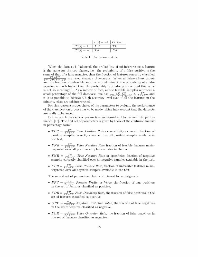
Assume to classify m unknown features in the two classes F , labelled with+1, and U , labelled with −1. Let C ∈ Rm be the vector with the correct featuresclassification, i.e. C(i) = 1 if the i-th feature xi ∈ F and C(i) = −1 if xi ∈ U ,i = 1, . . . ,m, and PC ∈ Rm the result of the classification process, i.e. PC(i) isthe predicted value of C(i), i = 1, . . . ,m.

For each feature four different situations can occur, that are illustrated inthe confusion matrix in Table 1:

• TP=true positive: C(i) = 1, PC(i) = 1 the feature is feasible and is cor-rectly classified,

• FP=false positive: C(i) = −1, PC(i) = 1 the feature is unfeasible but ismisinterpreted and classified as feasible,

• TN=true negative: C(i) = −1, PC(i) = −1 the feature is unfeasible andis correctly classified,

• FN= false negative: C(i) = 1, PC(i) = −1 the feature is feasible but ismisinterpreted and classified as unfeasible.

17

C(i) = −1 C(i) = 1PC(i) = 1 FP TPPC(i) = −1 TN FN

Table 1: Confusion matrix.

When the dataset is balanced, the probability of misinterpreting a featureis the same for the two classes, i.e. the probability of a false positive is thesame of that of a false negative, then the fraction of features correctly classified

TP+TNTN+TP+FN+FP is a good measure of accuracy. When unbalancedness occursand the fraction of unfeasible features is predominant, the probability of a falsenegative is much higher than the probability of a false positive, and this valueis not so meaningful. As a matter of fact, as the feasible samples represent asmall percentage of the full database, one has TP+TN

TN+TP+FN+FP 'TN

TN+FN andit is so possible to achieve a high accuracy level even if all the features in theminority class are misinterpreted.

For this reason a proper choice of the parameters to evaluate the performanceof the classification process has to be made taking into account that the datasetsare really unbalanced.

In this article two sets of parameters are considered to evaluate the perfor-mance, [18]. The first set of parameters is given by those of the confusion matrixin percentage form:

• TPR = TPTP+FN True Positive Rate or sensitivity or recall, fraction of

positive samples correctly classified over all positive samples available inthe test,

• FNR = FNTP+FN False Negative Rate fraction of feasible features misin-

terpreted over all positive samples available in the test,

• TNR = TNTN+FP True Negative Rate or specificity, fraction of negative

samples correctly classified over all negative samples available in the test,

• FPR = FPTN+FP False Positive Rate, fraction of unfeasible features misin-

terpreted over all negative samples available in the test.

The second set of parameters that is of interest for a designer is:

• PPV = TPTP+FP Positive Predictive Value, the fraction of true positives

in the set of features classified as positive,

• FDR = FPTP+FP False Discovery Rate, the fraction of false positives in the

set of features classified as positive,

• NPV = TNTN+FN Negative Predictive Value, the fraction of true negatives

in the set of features classified as negative,

• FOR = FNTN+FN False Omission Rate, the fraction of false negatives in

the set of features classified as negative.

18

Figure 6: Meaning of parameters PPV , FDR, NPV , FOR.

The meaning of these parameters is shown in Figure 6. When features areclassified by SVM they are divided into two subsets F , features classified aspositive, and U , features classified as negative. Parameter PPV interests thedesigner as gives a measure of the quality of set F , telling how many featuresare actually feasible, meaning that FDR = 1− PPV indicates how many use-less CFD computations will be performed at step 4 of Phase 1 and how manyoutliers could be part of the optimal solutions set at steps (4)-5 of Phase 2of Framework 3. On the other hand, another parameter to take into accountis FOR, which gives the percentage of feasible features in the set of featuresclassified as unfeasible, which are then wrongly discarded after the classificationprocess.

Notice that the couples (TPR,FNR), (TNR,FPR), (PPV, FDR), (NPV, FOR)sum up to one, so in the tables in Section 6 just a parameter for each couplewill be shown.

The dataset unbalancedness has to be taken into account also in meta-modeltraining. The designer is mainly interested in detecting feasible samples, so itis necessary to force the classifier to take features belonging to the differentclasses into different consideration. Generally the lack of balancedness of thedataset is handled using two different weights for the positive and the negativefeatures, to penalize with more severity the misinterpretation of feasible features,[25]. Coefficient C in the objective function (7) of the problem to be solvedduring SVM training is then split in C+ (coefficient for feasible features) andC− (coefficient for unfeasible features), so that the objective function becomes:

minω,b,ζ

1

2‖w‖2 + C+

∑xi∈F

ζi + C−∑xi∈U

ζi. (11)

To gain good results it is necessary to properly tune these coefficients, withthe aim of finding the better compromise between the need of detecting as manyfeasible features as possible and that of avoiding too many unfeasible featuresbeing classified as feasible ones, that would lead to useless CFD computationsin the regression process. In the literature, [25], it is suggested that the ratioof the coefficients corresponding to feasible and unfeasible features should be

19

inversely proportional to the ratio of the corresponding features set sizes:

C+

C−∼ |U||F|

, (12)

where |·| represents the cardinality of the set.In the next section it will be shown how all these considerations are taken

into account in practical parametric design tests.

6 Numerical results

In this section the results of the tests performed on three different databases,with different number of degrees of freedom and constraints, arising from thedescribed industrial application are reported. It is worth remembering that thebenefit granted by the proposed procedure compared to the one sketched inFramework 1 lays in the savings arising from the use of a classification meta-model, which makes the procedure practical. Moreover, the savings dependentirely on the classification process quality. Then in this section the focus ison the tuning of SVM free parameters to gain the best performance and on theresults obtained by the related classification process. The other steps of theprocedure are not shown, as this is out of the scope of the paper.

The SVM used to perform the tests is the one implemented by Chih-ChungChang and Chih-Jen Lin in LIBSVM - A Library for Support Vector Machines,[7]. The tests were performed calling the LIBSVM package through its MEXinterface, on a Intel Core(TM) i7-4510U 2.6 GHz, 8 GB RAM.

6.1 Experimental setting

In this section some details on the experimental setting and the data preparationare given.

For the tests the features are divided into two classes: class F of feasiblefeatures, corresponding to constructable machines and convergent CFD calcu-lations, and class U of unfeasible ones.

CFD calculations were carried out using the TRAF code [1], a steady/unsteady,multigrid/multiblock flow solver for the three-dimensional Reynolds-averagedNavier-Stokes equations. A detailed description of the numerical scheme canbe found in [1, 2]. The domain is divided in N cells. Denoted with R(n) theresiduals vector of the discretized equations on the n-th cell, for n = 1, . . . , N ,and with

R =1

N

N∑n=1

‖Ri(n)‖, (13)

the 2-norm of the residuals averaged on the total number of cells, the compu-tations are considered convergent if

log10R ≤ rescut (14)

20

where rescut is a suitable threshold fixed by the user. In the tests presentedbelow, it was set equal to one decade under the single precision machine zero,i.e. rescut = −8. If res(i) is the residual of the i-th feature,

• F = {xi|res(i) ≤ rescut},

• U = {xi|res(i) > rescut},

assuming res(i) = 0 for non-convergent computations or non-manufacturablemachines.

The data were prepared for the classification process, scaling the geometriesdegrees of freedom to have mean 0 and variance 1. In the literature indeed, itis known that a good scaling of both the training and the testing features isnecessary to have good results, otherwise the contribution of the features thathave a bigger values of some degree of freedom would be predominant over thecontributions of the other features.

A choice that deeply influence the performance of SVM learning algorithm, isthat of the kernel function (10). In LIBSVM many different choices are possible:linear, polynomial, radial basis function, sigmoid. For this specific applicationthe best performance was obtained with the radial basis function kernel:

K(x, y) = e−γ‖x−y‖2

,

where x, y are features and γ is a parameter to be set. A good choice of freeparameter γ is crucial. LIBSVM provides a tool to select it by a cross validationon a set of values. However when the dataset is large, cross validation can be areally time consuming process, so γ was determined using the default methodemployed in [28], [16], that is, it was set to the average squared distance amongtraining patterns.

For the tests the available data were divided into two subsets, a trainingset of mtrain = 30000 geometries and a validation set of mval = 50000 geome-tries, both composed of features of known classification. Notice that, even ifthe number of degrees of freedom is really high and a large number of pointsshould be necessary to accurately sample the design space, the chosen value oftraining features turned out to be sufficient to obtain good classification results.Increasing it, leads to higher training times without significant improvement inperformance.

6.2 Tests

For the numerical experimentation three different databases arising from theindustrial application introduced before are considered, which have respectivelyn=40, 44, 42 degrees of freedom, and for which the ratio between unfeasible and

feasible features |U||F| is 3:1, 7:1, 6:1.

The results of the tests are shown in Tables 2, 3 and 4, in which the pa-rameters described in Section 5 are reported, for many classification proceduresperformed with different choices of coefficient C+. Indeed, test were conducted

21

to investigate on the choice of the best combination of parameters. Then, pa-rameter C− = 1 was fixed, and different values of C+ were tested.

Looking at the tables it is possible to see that as C+ grows SVM is morereliable in detecting the feasible features, less and less feasible features are lost,as it is shown by the increasing value of TPR. On the other hand the model isless accurate in detecting the unfeasible features, and the number of false pos-itives increases: when C+ is large the machine identifies more feasible featuresbut among them there are more false positives than for smaller values of C+,as can be easily deduced by the decreasing value of PPV . So C+ should bebig enough to detect as many feasible solutions as possible and minimizing thenumber of feasible features lost due to the classification process (large TPR andsmall FOR), to form a reasonably large set of solutions to train the ANN, butnot too much, to keep the number of unfeasible features incorrectly classified asfeasible low (small FPR and high PPV ), to avoid useless CFD computationsand the performance evaluation of unfeasible geometries.

To investigate the choice of the best parameter combination a ROC curvecould be employed, [5]. In statistics, a Receiver Operating Characteristic, orROC curve, is a graphical plot that illustrates the performance of a binaryclassifier as a parameter is varied. The curve is created by plotting the truepositive rate (TPR) against the false positive rate (FPR) for different choicesof the free parameter. The best possible prediction would yield no false negativesand no false positives and would correspond to a point in the upper left cornerof coordinates (0,1) in the ROC space, while a random guess would give a pointalong the diagonal line from the left bottom corner to the top right one. Sopoints above the diagonal represent classification results better than randomones, while points below the line correspond to bad results, worse than random.The best results from a confusion matrix are then the closest to the upper leftcorner, and the distance from the random guess line can be used as an indicatorof how much predictive power a method has. In Figure 7 the ROC curvescorresponding to Table 2 (top left), Table 3 (top right) and to Table 4 (bottom)are reported. For each test it is possible to deduce the best values for the freeparameter, choosing the point closer to the upper left corner, which is markedby a black circle. Notice that these results are in good accordance with (12). Inthe tables then, the column corresponding to the best parameters combinationsis highlighted by bold font.

Table 2: Results of the classification tests performed on Dataset 1. Labelsmeaning is introduced in Section 5.

3 : 1 C+ = 1 C+ = 2 C+ = 3 C+ = 5 C+ = 10TPR 31.5% 66.1% 78.3% 88.5% 94.5%FPR 4.1% 15.4% 23.0% 33.1% 44.7%PPV 70.1 % 56.6% 50.8% 44.9 % 39.2 %FOR 17.9 % 10.9% 7.9% 5.0 % 2.9%

Then, independently of the choice of the parameter, even if SVM classifier

22

FPR

0 0.1 0.2 0.3 0.4 0.5 0.6 0.7 0.8 0.9 1

TP

R

0

0.1

0.2

0.3

0.4

0.5

0.6

0.7

0.8

0.9

1ROC Curve Dataset 1

C+

=1

C+

=2

C+

=3

C+

=5

C+

=10

FPR

0 0.1 0.2 0.3 0.4 0.5 0.6 0.7 0.8 0.9 1

TP

R

0

0.1

0.2

0.3

0.4

0.5

0.6

0.7

0.8

0.9

1ROC Curve Dataset 2

C+

=1

C+

=2

C+

=3

C+

=5

C+

=7

C+

=10

C+

=20

FPR

0 0.1 0.2 0.3 0.4 0.5 0.6 0.7 0.8 0.9 1

TP

R

0

0.1

0.2

0.3

0.4

0.5

0.6

0.7

0.8

0.9

1ROC Curve Dataset 3

C+

=1

C+

=2

C+

=3

C+

=5

C+

=7

C+

=10

C+

=20

Figure 7: ROC curve, Dataset 1 top left, Dataset 2 top right, Dataset 3 bottom.C+ weighting factor for feasible features, best value is highlighted by a blackcircle.

23

Table 3: Results of the classification tests performed on Dataset 2. Labelsmeaning is introduced in Section 5.

7 : 1 C+ = 1 C+ = 2 C+ = 3 C+ = 5 C+ = 7 C+ = 10 C+ = 20TPR 14.7% 53.5% 66.0% 77.5% 83.0% 86.5% 88.4%FPR 0.7% 5.9% 9.9% 16.1% 19.8% 23.1% 25.7%PPV 76.9% 58.5% 50.8% 42.7 % 39.4% 36.7 % 34.8 %FOR 11.7% 7.1% 5.5% 3.9 % 3.1% 2.6% 2.3 %

Table 4: Results of the classification tests performed on Dataset 3. Labelsmeaning is introduced in Section 5.

6 : 1 C+ = 1 C+ = 2 C+ = 3 C+ = 5 C+ = 7 C+ = 10 C+ = 20TPR 20.5% 55.5% 67.9% 78.7% 84.2% 87.2% 89.7%FPR 1.1% 6.1% 10.0% 15.0% 18.2% 20.7% 23.4%PPV 74.6 % 58.9% 51.8% 45.2% 42.1% 39.8% 37.6 %FOR 11.2 % 6.9 % 5.3% 3.8 % 2.9% 2.5% 2.1 %

allows in the feasible set a percentage of false positives, the general advantagegained by the use of the classification procedure is that it lowers the ratio be-tween unfeasible and feasible features in the set F that has to be tested by CFDcomputations. This new ratio is given by FDR

PPV . In all the tests it is much lowerthen the one in the original dataset. In the datasets considered the ratio turnsfrom 3:1 to about 1:1, from 7:1 to about 1.5:1 and from 6:1 to about 1.4:1. Thepractical outcome of this, is that when at step 2 of Phase 1 the design space issampled, the most part of the unfeasible geometries is discarded by SVM. Thenthe CFD are performed on dataset F which is an almost balanced dataset. Thesame benefits apply to Phase 2, when the regression meta-model is applied atstep (3) to F ′′ that, like F , is mainly composed of feasible features. Thus, thepresence of unfeasible geometries in the optimal solutions set is reduced and thecost of step (5) is lowered.

Let us show these benefits with a practical example. The same test as inSection 3.1 is used, which is the one considered in Table 3. Let us assume tohave tested with SVM enough features to have |F| ' 24600, which it is worthremembering is not an expensive procedure. Then, considering that for this testcase PPV = 50.8%, performing about 24600 CFD computations it is possibleto obtain a training set F ′ of about 12500 samples, the same size as the oneyielded by the procedure sketched in Framework 1, that was obtained with50000 computations (cfr. Section 3.1). The proposed approach allows then tosave more than 50% CFD computations to form the ANN training set. Moreoverthe result of step 2 of Phase 2 is a dataset F ′′ in which just half of the featureswill result to be unfeasible, so it is less likely to obtain optimal solutions setscomposed just of unfeasible features.

Similar remarks can be made for the others datasets. In that cases, due to

24

Table 5: Results of the classification tests performed on Dataset 1 with optimalvalue of γ.

3:1 C+ = 1 C+ = 2 C+ = 3 C+ = 5 C+ = 10TPR 32.7% 66.2% 78.2% 88.0% 93.8%FPR 4.3% 15.4% 22.8% 32.5% 43.1%PPV 70.0 % 56.6% 51.1% 45.2 % 39.8 %FOR 17.6 % 10.8 % 7.9% 5.1 % 3.2 %

the stronger unbalancedness, the savings in CFD computations are even higher,around 67%.

Notice also that the percentage of feasible features in the set of features clas-sified as unfeasible (and then wrongly discarded after the classification process)is low, about 8% for Dataset 1 and 3% or the other two.

All of this, leads to conclude that the proposed procedure is actually effectivein reducing the computational costs and improves the previously consideredapproach.

The strategy chosen to handle the dataset unbalancedness shows to be ef-fective, SVM classification meta-model performs well and allows to successfullyhandle problems with different unbalancedness levels. In fact, even if the lasttwo classification problems are more difficult than the first, with a suitablechoice of parameter C+ good results are obtained.

Finally, it is worth noticing that in all the tests presented above, indepen-dently of the dataset considered, the same value γ = 0.0114 is used. Findingthe right value for the free parameter, using either a cross-validation or theaverage squared distance among training patterns is rather a time consumingcomputation, that should be performed each time the dataset is varied. It isconvenient to use the same parameter to build models also for different kind ofmachines, to save computational time and to have a tool that does not need tobe tuned on each test case. The γ value that was used in the tests is optimizedfor the dataset with n = 44 degrees of freedom. While the optimal parameterfor the dataset with n = 42 degrees of freedom is quite the same, the optimalone for the other dataset is γ = 0.0135. In Table 5 the results obtained withthe optimal parameter γ = 0.0135 for the dataset with 40 degrees of freedomare reported. Comparing them with those in Table 3, it is possible to see thatthey do not change significantly, so the same parameter γ can be used for allthis dataset without loss of accuracy.

7 Conclusions and remarks

In this article a hybrid approach to face the parametric design of a centrifugalpump is presented, which is based on coupling CFD computations, SVM classi-fication and ANN regression. An intrinsic property of a parametric design is thepresence of many unfeasible geometries in the design space, so that the databasesformed according to the parameterization chosen are really unbalanced. This

25

has two main drawbacks. On one hand, a huge number of CFD computationsis necessary to form a suitable training set for the regression meta-model. Onthe other hand, the optimal solutions set found evaluating the performancefunctions of new samples by means of the trained meta-model, could be madejust of unfeasible geometries. A strategy to solve these two problems, basedon coupling the regression process with a classification by SVM, is presented.The strategy was tested on various datasets with a large number of degrees offreedom, different constraints and different ratio between feasible and unfeasi-ble features. It is shown that with a fine tuning of the free parameters differentunbalancedness levels can be handled. Moreover, the use of the classificationprocedure allows to discard the most part of the unfeasible samples, making thedesign procedure doable and cutting the number of required CFD computationsby about 50%− 70%.

References

[1] A. Arnone. Viscous analysis of three-dimensional rotor flow us-ing a multigrid method. Journal of Turbomachinery, 116(3):435–445,doi:10.1115/1.2929430, 1994.

[2] A. Arnone. Multigrid methods for turbomachinery navier-stokes calcula-tions. In Solution Techniques for Large-Scale CFD Problems, pages 293–332. John Wiley and Sons, New York, 1995.

[3] A. Arnone and R. Pacciani. Three-dimensional viscous analysis of centrifu-gal impellers using the incompressible navier-stokes equations. In Proceed-ings of 1st European Conference on Turbomachinery, Erlangen, Germany,pages 181–195, 1995.

[4] D. Bonaiuti, A. Arnone, M. Ermini, and L. Baldassarre. Analysis andoptimization of transonic centrifugal compressor impellers using the de-sign of experiments technique. Journal of Turbomachinery, 128(4):786–797,doi:10.1115/1.1579507, 2006.

[5] A.P. Bradley. The use of the area under the roc curve in the evaluationof machine learning algorithms. Pattern Recognition, 30(7):1145–1159, doi:10.1016/S0031–3203(96)00142–2, 1997.

[6] C. Chahine, J. R. Seume, and T. Verstraete. The influence of metamod-eling techniques on the multidisciplinary design optimization of a radialcompressor impeller. In Proceedings of ASME Turbo Expo 2012, 11-15June 2012, Copenhagen, Denmark, pages 1951–1964. doi:10.1115/GT2012-68358, 2012.

[7] C.C. Chang and C.J. Lin. Libsvm: a library for support vector machines.ACM Transactions on Intelligent Systems and Technology, 2(3):Article No.27, 2011.

26

[8] M. Checcucci, F. Sazzini, M. Marconcini, A. Arnone, M. Coneri,L. De Franco, and M. Toselli. Assessment of a neural-network-based op-timization tool: a low specific-speed impeller application. InternationalJournal of Rotating Machinery, 2011, doi:10.1155/2011/817547, 2011.

[9] M. Checcucci, A. Schneider, M. Marconcini, F. Rubechini, A. Arnone,L. De Franco, and M. Coneri. A novel approach to parametric design ofcentrifugal pumps for a wide range of specific speeds. In Conference: 12thInternational Symposium on Experimental and Computational Aerother-modynamics of Internal Flows, 13-16 July 2015, Lerici (SP), Italy, pageISAIF 12 paper nr.121, 2015.

[10] L. Ellbrant, L.E. Eriksson, and H. Martensson. Design of compressor bladesconsidering efficiency and stability using cfd based optimization. In Proceed-ings of ASME Turbo Expo 2012, 11-15 June 2012, Copenhagen, Denmark,pages 371–382. doi:10.1115/GT2012-69272, 2012.

[11] S. Haykin. Neural Networks: A Comprehensive Foundation. 2nd edition.Macmillan, New York, ISBN: 978-0780334946, 1998.

[12] P.H. Hergt. Pump research and development: Past, present, and future.Journal of Fluids Engineering, 121(2):248–253, doi: 10.1115/1.2822198,1999.

[13] H. Liu, K. Wang, S. Yuan, M. Tan, Y. Wang, and L. Dong. Multiconditionoptimization and experimental measurements of a double-blade centrifugalpump impeller. Journal of Fluids Engineering, 135(1):0111031–01110313,doi: 10.1115/1.4023077, 2013.

[14] Dingguo Lu and Wei Qiao. A ga-svm hybrid classifier for multiclass faultidentification of drivetrain gearboxes. In Energy Conversion Congress andExposition (ECCE), 2014, pages 3894–3900. IEEE, 2014.

[15] J. Monedero. Parametric design: a review and some experiences. Automa-tion in Construction, 9(4):369–377, 2000.

[16] R. Nanculef, E. Frandi, C. Sartori, and H. Allende. A novel frank–wolfe al-gorithm. analysis and applications to large-scale svm training. InformationSciences, 285:66–99, doi:10.1016/j.ins.2014.03.059, 2014.

[17] S. Nandi, Y. Badhe, J. Lonari, U. Sridevi, B.S. Rao, S.S. Tambe, and B.D.Kulkarni. Hybrid process modeling and optimization strategies integratingneural networks/support vector regression and genetic algorithms: Study ofbenzene isopropylation on hbeta catalyst. Chemical Engineering Journal,97(2):115–129, doi:10.1016/S1385–8947(03)00150–5, 2004.

[18] D. L. Olson and D. Delen. Advanced Data Mining Techniques. SpringerScience & Business Media, ISBN 978-3-540-76917-0, 2008.

27

[19] E. Osuna, R. Freund, and F. Girosit. Training support vector machines: anapplication to face detection. In Proceedings of Computer Society Confer-ence on Computer Vision and Pattern Recognition 1997, 17-19 June 1997,Puerto Rico, pages 130–136. IEEE, 1997.

[20] S. Pierret. Turbomachinery blade design using a navier-stokes solver andartificial neural network. ASME Journal of Turbomachinery, 121(3):326–332, doi:10.1115/1.2841318, 1999.

[21] F. Rubechini, A. Schneider, A. Arnone, S. Cecchi, and F. A. Malavasi. Aredesign strategy to improve the efficiency of a 17-stage steam turbine. InProceedings of ASME Turbo Expo 2009, 812 June 2009, Orlando, Florida.,pages 1463–1470. doi:10.1115/GT2009-60083, 2009.

[22] F. Rubechini, A. Schneider, A. Arnone, F. Dacca C. Canelli, andP. Garibaldi. Aerodynamic redesigning of an industrial gas turbine. InProceedings of ASME Turbo Expo 2011, 6-10 June 2011, Vancouver, BC,pages 1387–1394. doi:10.1115/GT2011-46258, 2011.

[23] B. Scholkopf and A. J. Smola. Learning with Kernels: Support VectorMachines, Regularization, Optimization, and Beyond. MIT Press, ISBN:9780262194754, 2001.

[24] D.H. Seo, T.S. Roh, and D.W. Choi. Defect diagnostics of gas tur-bine engine using hybrid svm-ann with module system in off-design con-dition. Journal of Mechanical Science and Technology, 23(3):677–685,doi:10.1007/s12206–008–1120–3, 2009.

[25] H. Shin and S. Cho. How to deal with large dataset, class imbalance andbinary output in svm based response model. In Proceedings of the KoreanData Mining Conference, pages 93–107, 2003.

[26] F. EH. Tay and L. Cao. Application of support vector machines in fi-nancial time series forecasting. Omega, 29(4):309–317, doi:10.1016/S0305–0483(01)00026–3, 2001.

[27] S. Tong and D. Koller. Support vector machine active learning with ap-plications to text classification. Journal of Machine Learning Research,2(11):45–66, doi:10.1162/153244302760185243, 2001.

[28] I. W. Tsang, J. T. Kwok, and P.M. Cheung. Core vector machines: Fastsvm training on very large data sets. Journal of Machine Learning Research,6:363–392, 2005.

[29] A. Veress and R. Van den Braembussche. Inverse design and optimizationof a return channel for a multistage centrifugal compressor. Journal ofFluids Engineering, 126(5):799–806, doi:10.1115/1.1792258, 2004.

28