Support Vector Machines for Direction

of Arrival Estimation

Judd A. Rohwer∗ and Chaouki T. Abdallah†

1 Abstract

Machine learning research has largely been devoted to binary and multiclassproblems relating to data mining, text categorization, and pattern/facial recog-nition. Recently, popular machine learning algorithms have successfully beenapplied to wireless communication problems, notably spread spectrum receiverdesign, channel equalization, and adaptive beamforming with direction of arrivalestimation (DOA). Various neural network algorithms have been widely appliedto these three communication topics. New advanced learning techniques, such assupport vector machine (SVM) have been applied, in the binary case, to receiverdesign and channel equalization. This paper presents a multiclass implemen-tation of SVMs for DOA estimation and adaptive beamforming, an importantcomponent of code division multiple access (CDMA) communication systems.

2 Introduction

Machine learning techniques have been applied to various problems relating tocellular communications. In our research we present a machine learning basedapproach for DOA estimation in a CDMA communication system [1]. TheDOA estimates are used in adaptive beamforming for interference suppression,a critical component in cellular systems. Interference suppression reduces themultiple access interference (MAI) which lowers the required transmit power.The interference suppression capability directly influences the cellular systemcapacity, i.e., the number of active mobile subscribers per cell.

Beamforming, tracking, and DOA estimation are current research topics withvarious technical approaches. Least mean square estimation, Kalman filtering,and neural networks [2],[3],[4], have been successfully applied to these problems.

∗Sandia National Laboratories P.O. Box 5800, MS-0986 Albuquerque, NM 87185-0986:jarohwe@sandia.gov

†C.T. Abdallah is with the Department of Electrical and Computer Engineering, Universityof New Mexico, Albuquerque, NM 87131, USA; chaouki@eece.unm.edu

0Sandia is a multiprogram laboratory operated by Sandia Corporation, a Lockheed MartinCompany, for the United States Department of Energy under Contract DE-AC04-94AL85000.

1

Many approaches have been developed for calculating the DOA; three techniquesbased on signal subspace decomposition are ESPRIT, MUSIC, and Root-MUSIC[1].

Adaptive antenna arrays are critical components of a wireless communicationsystem. System designers utilize state of the art signal processing techniques foradaptive beamforming and interference suppression. Research in this area showsthat it is possible to direct the maximum antenna gain towards the desired signaland to effectively place nulls in the direction of interfering users. By adaptivelyupdating the antenna array weights the desired signal can be tracked, keepingcontinuous coverage and maintaining the largest possible signal-to-interference(SIR) ratio. The adaptive antenna arrays must be able to process multipleDOAs of the desired signal.

Neural networks have been successfully applied to the problem of DOAestimation and adaptive beamforming in [4], [5], [6]. New machine learningtechniques, such as support vector machines (SVM) and boosting, perform ex-ceptionally well in multiclass problems and new optimization techniques arepublished regularly. These new machine learning techniques have the potentialto exceed the performance of the neural network algorithms relating to com-munication applications. Specifically the techniques applied DOA estimationand adaptive beamforming will increase the speed of convergence to the desiredantenna array weights and decrease the time necessary for system training.

In our research machine learning is applied to two areas of adaptive antennaarrays; the estimation of the array weight vectors, Wi.r , and the DOA esti-mates, θr . The goal is to minimize the interference which in turn will improvethe quality of service (QoS) and increase cellular system capacity. To reducethe interference power the adaptive array system focuses the beam towards thedesired user and effectively places nulls in the direction of the interferers. In aCDMA system the beamwidth, maximum directivity, and nulls do not requireextreme accuracy, as would be required for frequency division multiple access(FDMA) systems. The machine learning methods presented in this paper in-clude subspace based estimation applied to the sample covariance matrix of thereceived signal. The optimization techniques use both training data and re-ceived data to generate the DOA estimates and antenna weight vectors. Theend result is an efficient machine learning approach to finding the DOA esti-mates which are applied to a Rake receiver based CDMA cellular architecture[1]. This cellular base station design with Rake receivers maximizes the receivedSIR, reduces multiple access interference (MIA), and thus reduces the requiredtransmit power from the mobile subscriber. If a system includes R Rake fingersthen the machine learning algorithms must estimate the L dominated signalpaths for each Rake finger.

Many computational techniques exist for working through limitations ofDOA estimation techniques, but currently no techniques exist for a system levelapproach to accurately estimating the DOAs at the base station. A number oflimitations relating to popular DOA estimation techniques are: 1) the signalsubspace dimension is not known, many papers assume that it is. The differ-

2

ences in eigenvalues between the covariance matrix and the sample covariancematrix add to the uncertainty, 2) searching all possible angles to determine themaximum response of the MUSIC algorithm, 3) evaluating the Root-MUSICpolynomial on the unit circle, 4) multiple eigen decompositions for ESPRIT, 5)computational complexity for maximum likelihood method.

This paper is organized as follows. Section 3 presents the system modelsfor an adaptive antenna array CDMA systems. A review of machine learningis presented in Section 4. In Section 5 we present background information onbinary and multiclass SVMs. Finally, Section 6 presents a multiclass SVMalgorithm for DOA estimation and simulation results.

3 System Models

This section includes an overview of system models for the received signal andadaptive antenna arrays designs. All notation is described below and is consis-tently used throughout the paper.

3.0.1 Received Signal at Antenna Array output

The signal from antenna array A, detected at the adaptive array processor is

xA (t) =J∑

j=1

L∑

l=1

√ptj (t) gji (t)a (θl) ql

jsj (t− τ j) cos (wc (t− τ j)) + nj (t) . (1)

xA (t) is the signal vector from antenna array Aptj (t) is the transmit signal power from mobile j.gji (t) is the link gain from base j to mobile i.qlj is the attenuation due to shadowing from path l.

a (θl) =[

1 e−jkl . . . e−j(D−1)kl]T

is the D × 1 steering vector.kl = νwo

c sin θl

θlis the direction of arrival of the l signal.D is the number of elements in the array.sj (t− τ j) is the CDMA spreading code.τ j is the propagation delay from mobile j to the base station.nj (t) is the additive white Gaussian noise for mobile j′s received signal.J is the number of received signals; One desired and J−1 interfering signals.L is the number of transmission paths.The spreading code is generated by

sj (t− τ j) =Sc∑

n=1

bj (n) cj (t− nT ) . (2)

bj (t) is the baseband signal of mobile j.cj (t) is the CDMA spreading code of mobile j.Sc is the number of chips in the spreading code.

3

T is the time period of one chip.To ease the complexity of the notation the terms relative to the multiple

paths are combined as

zj =L∑

l=1

a (θl) qlj . (3)

In [7] zj is defined as the spatial signature of the antenna array to the jth source.The signal vector from the antenna array is rewritten as

xA (t) =J∑

j=1

√ptj (t) gji (t)zjsj (t− τ j) cos (wc (t− τ j)) + nj (t) . (4)

3.0.2 Received Signal at Rake Receivers

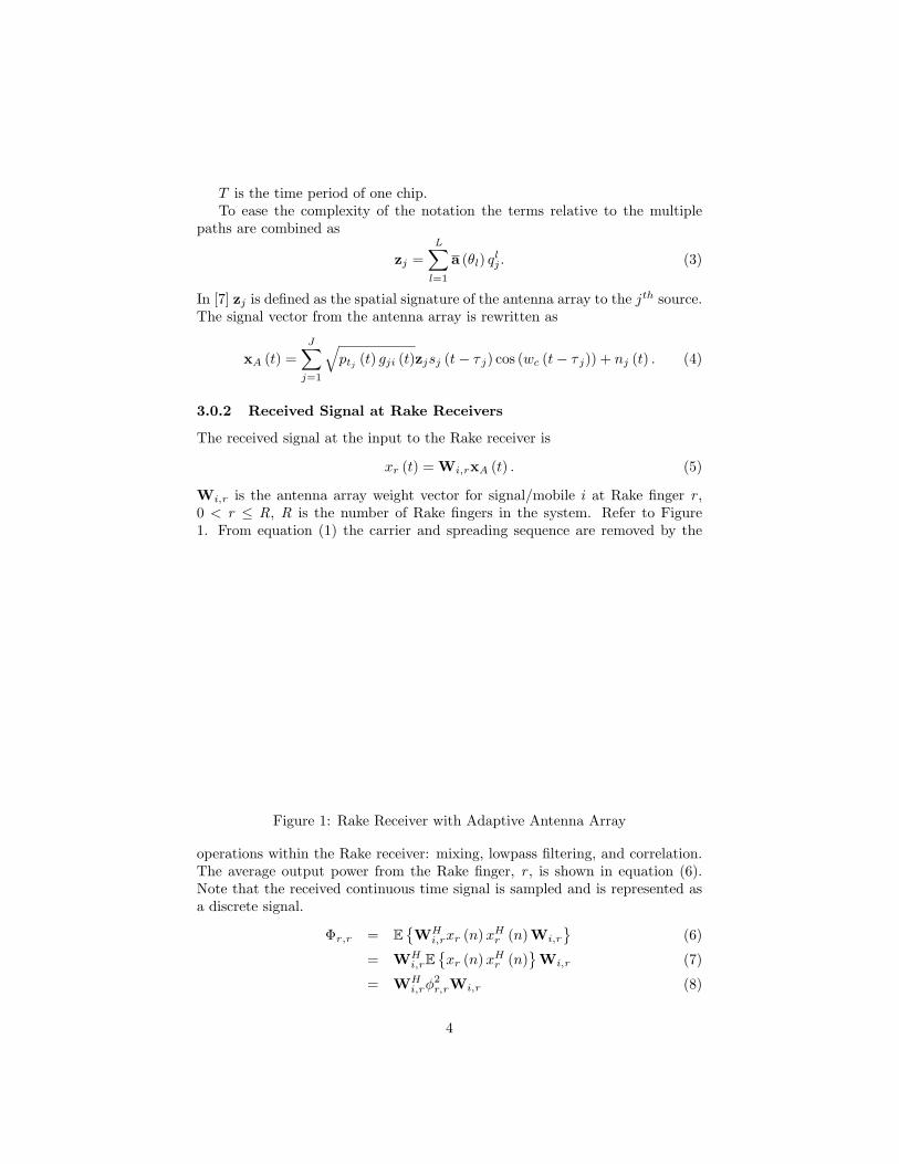
The received signal at the input to the Rake receiver is

xr (t) = Wi,rxA (t) . (5)

Wi,r is the antenna array weight vector for signal/mobile i at Rake finger r ,0 < r ≤ R, R is the number of Rake fingers in the system. Refer to Figure1. From equation (1) the carrier and spreading sequence are removed by the

Figure 1: Rake Receiver with Adaptive Antenna Array

operations within the Rake receiver: mixing, lowpass filtering, and correlation.The average output power from the Rake finger, r , is shown in equation (6).Note that the received continuous time signal is sampled and is represented asa discrete signal.

Φr ,r = EWH

i,rxr (n) xHr (n)Wi,r

(6)

= WHi,rE

xr (n) xH

r (n)Wi,r (7)

= WHi,rφ

2r,rWi,r (8)

4

WHi,r is the Hermitian transpose of Wi,r , xH

r (n) is the Hermitian transposeof xr (n) .In equation (8) φ2

r ,r is the autocorrelation of the received signal andis defined below.

φ2r ,r = φ2

s,r + φ2I+N,r (9)

φ2s,r = pti

giizizHi (10)

φ2I+N,r =

J∑

j 6=i

ptj gjizjzHj + niI (11)

The received power is rewritten in equations (12) - (15).

Φr,r = WHi,r

(φ2

s,r + φ2I+N,r

)Wi,r (12)

= WHi,rφ

2s,rWi,r + WH

i,rφ2I+N,rWi,r (13)

= ptigHii W

Hi,rzizH

i Wi,r

+J∑

j 6=i

ptj gHjiW

Hi,rzjzH

j Wi,r + niWHi,rWi,r (14)

Φr,r = Φs,r + ΦI+N,r (15)

From the above equations the SIR at the output of each Rake receiver is

SIRi,r = γi,r =Φs,r

ΦI+N,r=

ptigiiWHi,rzizH

i Wi,r∑Jj 6=i ptj gjiWH

i,rzjzHj WH

i,r + niWHi,rWi,r

. (16)

The composite SIRi is taken at the output of the diversity combiner, in generalfor an equal gain combiner SIRi =

∑Rr=1 SIRi,r . Refer to [1] for information on

various diversity combining techniques. The goal of adaptive beamforming is tomaximize the power of the received signal, Φs,r , and minimize the interferenceand noise power, ΦI+N,r , by finding the optimum antenna array weights Wi,r

for each rake receiver.

3.0.3 Machine Learning for DOA Estimation

From the system model in Section 3.0.2 the solution for the optimal weightvector [7], [8], is

Wi,r =Φ−1

I+N,rzi

zHi Φ−1

I+N,rzi

(17)

With principal component analysis and machine learning we can estimate theinterference, ΦI+N,r , and the array response, zj =

∑Ll=1 a (θl) ql

j .To estimate the array response, zi, we must know a (θl) and ql

i. The continu-ous pilot signal, included in cdma2000, can be used in estimating ql

i. This mustbe done for each resolvable path, i.e., qi =

[q1i , q2

i , . . . , qLi

]. Estimating

A (θ) =[

a (θ1) , a (θ2) , . . . ,a (θL)]

requires information on the DOA.

5

The process of DOA estimation is to monitor the outputs of D antennaelements and predict the angle of arrival of L signals, L < D . The outputmatrix from the antenna elements is

A =[

a (θ1) a (θ2) . . . a (θL)]

(18)

a (θl) =[

1 e−jkl e−j2kl . . . e−j(D−1)kl]T

, (19)

and the vector of incident signals is θr =[

θ1, θ2, . . . , θL

]. With a train-

ing process the learning algorithms generate DOA estimates, θr =[

θ1, θ2, . . . , θL

],

based on the responses from the antenna elements, a (θl).

4 Machine Learning Background

Machine learning has already made an impact in the analysis and design ofcommunication systems. Neural Networks are applied to numerous problems,ranging from adaptive antenna arrays [4], multiuser receiver design [9],[10], in-terference suppression [11], and power prediction [12]. Designs with SVMs arestarting to appear in the journals [13],[14]. Boosting algorithms have been ap-plied to standard classification problems, such as text and image classification,but have yet to be applied to specific communication problems.

Machine learning is the process of observing input data and applying classifi-cation rules to generate a binary or multiclass label to the output. In the binarycase a classification function is estimated using input/output training pairs withunknown probability distribution, P (x, y), x is sample vector of observations,and

(x1,y1), . . . , (xn,yn) ∈ RN × Y, (20)yi = −1, +1 . (21)

The estimated classification function maps the input to a binary output, f :RN → −1,+1 . The system is first trained with the input/output data pairsthen the test data, from the same probability distribution P (x, y), is appliedto the classification function. The binary output label, +1, is generated iff(x) ≥ 0, likewise −1 is the output label if f(x) < 0. For the multiclass caseY ∈ RG where Y is a finite set of real numbers and G is the size of the multiclasslabel set. The objective is to estimate the function which maps the input datato a finite set of output labels f : RN → G

(RN

) ∈ RG

Estimating the classification function is approached by minimizing the ex-pected risk [15]. The risk is defined as

R [f ] =∫

L (f (x) , y) dP (x, y). (22)

The loss function, L, is explained in [15]. Since the probability distribution ofthe input data is unknown the classification function must be estimated. The

6

estimation process is based on empirical risk minimization.

Remp [f ] =1n

l∑

i=1

(f (xi) , yi) (23)

By setting conditions of the minimization routine the empirical risk convergestowards the expected risk. Minimization routines must be carefully selectedso the generalization (test) error closely tracks the training error. Overfittingoccurs when small sample (test) sizes generate large deviations in the empiricalrisk; the problem of overfitting can be minimized by restricting the complexityof the function class from which the classification function is chosen. For adetailed synopsis of this area of research review the Vapnik-Chervonenkis (VC)theory and structural risk minimization (SRM) [16].

The general process of SVM algorithms is to project the input space to ahigher feature space via a nonlinear mapping,

Γ : RN → z (24)x 7→ Γ (x) . (25)

The input data x1, . . . ,xn ∈ RN is mapped into a new feature space z whichcould have a much higher dimensionality. The data in the new feature space isthen applied to the desired machine learning algorithm. For the binary case theinput/output pairs in new feature space are described as

(Γ (x1) ,y1), . . . , (Γ (xn) ,yn) ∈ z× Y. (26)

The background of machine learning shows that the dimension of the featurespace is not as important as the complexity of the classification functions. Forexample in the input space the input/output pairs may be represented with anonlinear function, but in a higher dimension feature space the input/outputpairs may be separated with a linear hyperplane.

4.1 Kernel Functions

Kernel functions are used to compute the scalar dot products of the input/outputpairs in the feature space z. Without kernel functions it might be impossible toperform scalar operations in the higher dimensional feature space. Essentially,an algorithm in the input space can be applied to the data in the feature space.

Γ (x) ·Γ (y) = k (x,y) (27)

Therefore a linear algorithm in the feature space corresponds to a nonlinearalgorithm, such as the classification functions, in the input space. This allowsa decision rule to be applied to the inner product of training points and testpoints in the feature space.

7

Three popular kernel functions are the linear kernel, polynomial kernel, ra-dial basis function (RBF), and multilayer perceptrons (MLP).

linear → k (x,y) = x · y (28)

polynomial of degree d → k (x,y) = ((x · y)+θ)d (29)

RBF → k (x,y) = exp

(−‖x− y‖2

σ2

)(30)

MLP → k (x,y) = tanh (κ (x · y)+θ) (31)

The performance of each kernel function varies with the characteristics of theinput data. Refer to [17] for more information on feature spaces and kernelmethods.

5 Support Vector Machines - Background

SVMs were originally designed for the binary classification problem. A varietyof approaches are currently being developed to tackle the problem of applyingSVMs to multiclass problems. Much like all machine learning algorithms SVMsfind a classification function that separates the hyperplane with the largest mar-gin. This is the difference between all machine learning algorithms, the math-ematical operations involved in calculating the optimal separating hyperplane.The SVM maps an inner product of the input space into a higher dimensionalfeature space via a kernel operation. The projected data does not have thefull dimensionality of the feature space since the mapping process is to a non-unique generalized surface [14]. The data points near the optimal hyperplaneare the “support vectors” and serve as the basis of the feature space. ThereforeSVMs are a nonparametric machine learning algorithm with the capability ofcontrolling the capacity through the support vectors.

5.1 Binary Classification

In binary classification system the machine learning algorithm produces esti-mates with a hyperplane separation, i.e.,yi ε [−1, 1] represents the classification“label” of the input vector x . The input sequence and a set of training labelsare represented as xk,ykK

k=1 , yk = −1, +1 . If the two classes are linearlyseparable in the input space then the the hyperplane is defined as wx+b = 0,w is a vector of weights and b is a bias term, if the input space is projected to ahigher dimensional feature space then the hyperplane becomes wΓ (x)+b = 0.

The nonlinear function Γ (·) : RN → RN′

maps the input space to the featurespace.

8

5.1.1 Support Vector Machines

The SVM algorithm is based on the assumption [18] that

wT Γ (xk)+b ≥ 1, if yk = +1, (32)wT Γ (xk)+b ≤ −1, if yk = −1. (33)

This formulation is restated as yk

[wT Γ (xk)+b

] ≥ 1, k = 1, . . . ,K.The SVM optimization is defined as

minw,b,φ

L (w,φ) =12‖w‖2 + c

K∑

k=1

φk, with constraints (34)

yk

[wT Γ (xk)+b

] ≥ 1− φk, k = 1, . . . , K (35)φk ≥ 0, k = 1, . . . ,K. (36)

Misclassifications, due to overlapping distributions, are accounted for with theslack variables φk, c is a tuning parameter. The margin between the hyperplaneand the data points in the feature space is maximize when w is minimized. Thesolution to the optimization problem in (34) is given by the saddle point of theLagrangian function,

Z (w,b,φ, α, ε) = L (w,φ)−K∑

k=1

αk

yk

[wT Γ (xk)+b

]− 1 + φk

−K∑

k=1

εkφk

(37)where αk ≥ 0 and εk ≥ 0 are Lagrangian multipliers. By computing

maxα,ε

minw,b,φ

Z (w,b,φ, α, ε) , (38)

the dual Lagrangian problem is developed; differentiating with respect to w,b,φ,[17], [18] leads to

dZdw

= 0, w =K∑

k=1

αkykΓ (xk) (39)

dZdb

= 0,

K∑

k=1

αkyk = 0 (40)

dZdφ

= 0, 0 ≤ αk ≤ c, k = 1, . . . , K. (41)

The classic quadratic programming problem is developed by replacing w in theLagrangian:

maxα

Ω(α) = −12

K∑

k,j=1

αkαjykyjk(xk,xj

)+

K∑

k=1

αk, such that (42)

K∑

k=1

αkyk = 0, 0 ≤ αk ≤ c, k = 1, . . . , K. (43)

9

The kernel function, described in Section 4.1, is k(xk,xj

)= Γ (xk) ·Γ (xj) . The

kernel should be chosen in order to eliminate the need to calculate w and Γ (x).From the developments above the nonlinear SVM is defined as

y (x) = sign

[K∑

k=1

αkykk (x,xk) + b

]. (44)

The non-zero α′ks are “support values” and the corresponding data points arethe “support vectors”. The support vectors are located close to the hyperplaneboundary. The test data x is projected onto the training vectors xk The sum-mation of the multivariable product of the support values, binary labels andthe feature space projection products the corresponding test label. This SVMbinary classification algorithm is used to produce larger multiclass classificationalgorithms.

5.1.2 Sequential Minimal Optimization (SMO)

Numerous algorithms have been developed for training SVMs. The SMO algo-rithm is an optimization routine for the quadratic programming (QP) problem,equation (42) , where the large scale QP problem is decomposed into smaller,manageable QP problems. The small QP problems are solved analytically versuslarge scale QP optimization routines. This approach promotes the sparseness ofthe data sets, created by the zero-valued support vectors. SMOs have minimumtraining time which is linear with respect to the training set size, the maxi-mum training time is quadratic with the training set size. This can be ordersof magnitude less than other training algorithms presented in current research,such as the projected conjugate gradient (PCG) chunking method and SVMlight

[19],[20]. The SMO algorithm reduces the complexity and improves the trainingtime of SVMs, all of which makes SVMs more user friendly and attractive tomany applications. Refer to [19] for pseudo code of SMO algorithm.

5.1.3 Least Squares SVM

Suykens, et.al., [21] introduced a least squares SVM (LS-SVM) which is basedon the Vapnik SVM classifier discussed in Section 5.1.1 and repeated below inequation (45) .

y (x) = sign

[K∑

k=1

αkykk (x,xk) + b

](45)

The LS-SVM classifier is generated from the optimization problem:

minw,b,φ

LLS (w,b,φ) =12‖w‖2 +

12ψ

K∑

k=1

φ2k, with constraints (46)

yk

[wT Γ (xk)+b

] ≥ 1− φk, k = 1, . . . , K (47)

10

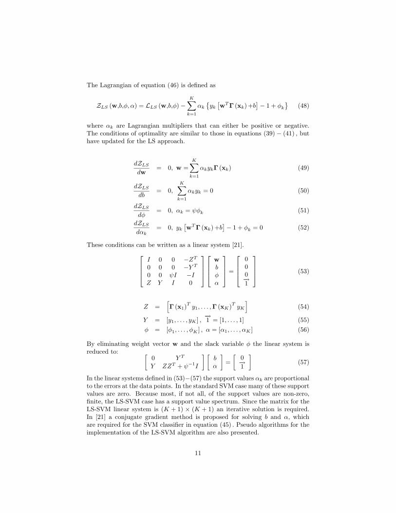
The Lagrangian of equation (46) is defined as

ZLS (w,b,φ, α) = LLS (w,b,φ)−K∑

k=1

αk

yk

[wT Γ (xk)+b

]− 1 + φk

(48)

where αk are Lagrangian multipliers that can either be positive or negative.The conditions of optimality are similar to those in equations (39)− (41) , buthave updated for the LS approach.

dZLS

dw= 0, w =

K∑

k=1

αkykΓ (xk) (49)

dZLS

db= 0,

K∑

k=1

αkyk = 0 (50)

dZLS

dφ= 0, αk = ψφk (51)

dZLS

dαk= 0, yk

[wT Γ (xk)+b

]− 1 + φk = 0 (52)

These conditions can be written as a linear system [21].

I 0 0 −ZT

0 0 0 −Y T

0 0 ψI −IZ Y I 0

wbφα

=

000−→1

(53)

Z =[Γ (x1)

Ty1, . . . ,Γ (xK)T

yK

](54)

Y = [y1, . . . , yK ] ,−→1 = [1, . . . , 1] (55)

φ = [φ1, . . . , φK ] , α = [α1, . . . , αK ] (56)

By eliminating weight vector w and the slack variable φ the linear system isreduced to: [

0 Y T

Y ZZT + ψ−1I

] [bα

]=

[0−→1

](57)

In the linear systems defined in (53)−(57) the support values αk are proportionalto the errors at the data points. In the standard SVM case many of these supportvalues are zero. Because most, if not all, of the support values are non-zero,finite, the LS-SVM case has a support value spectrum. Since the matrix for theLS-SVM linear system is (K + 1) × (K + 1) an iterative solution is required.In [21] a conjugate gradient method is proposed for solving b and α, whichare required for the SVM classifier in equation (45) . Pseudo algorithms for theimplementation of the LS-SVM algorithm are also presented.

11

5.2 Multiclass Classification

There exist many SVM approaches to multiclass classification problem. Twoprimary techniques are one-vs-one and one-vs-rest. One-vs-one applies SVMs toselected pairs of classes. For P distinct classes there are P(P−1)

2 hyperplanes thatseparate the classes with maximum margin. The one-vs-rest SVM techniquegenerates P hyperplanes that separate each distinct class from the ensemble ofthe rest. In this paper we only consider the one-vs-one multiclass SVM.

For the multiclass problem the machine learning algorithm produces esti-mates with multiple hyperplane separations,. The set of input vectors andtraining labels is defined as xn,yg

nn=N,g=Gn=1,g=1 , xn ∈ RN, n = 1, . . . , N, yi ∈

1, . . . , G , n is the index of the training pattern and G is the number of classes.One-vs-one multiclass classification is based on the binary SVMs discussed in

Sections 5.1 and 5.1.3. In the training phase the margins for P(P−1)2 hyperplanes

are constructed. The basic approach uses a tree structure to compare the testdata to each of the P(P−1)

2 hyperplanes. Through a series of elimination stepsthe best label is assigned to the input data. The Decision Directed AcyclicGraph (DDAG) and DAGSVM are specific techniques for one-vs-one multiclassclassification; a review of each is included below.

5.2.1 DDAG and DAGSVM

Platt, et.al., [22] introduced the DDAG, a VC analysis of the margins, andthe development of the DAGSVM algorithm. The two techniques are based onP(P−1)

2 classifiers for a P class problem, one classifier for each pair of classes.The DAGSVM includes an efficient one-vs-one SVM implementation that allowsfor faster training than the standard one-vs-one algorithm and the one-vs-restapproach.

The DDAG algorithm includes P(P−1)2 nodes, each associated with a one-

vs-one classifier and it’s respective hyperplane. The test error of the DDAGdepends on the number of classes, P , and the margins at each node. In [22] it isproved that maximizing the margins at each node of the DDAG will minimizedthe generalization error, independently of the dimension of the input space.Likewise, the input data is projected to a higher dimension feature space usingappropriate kernel functions.

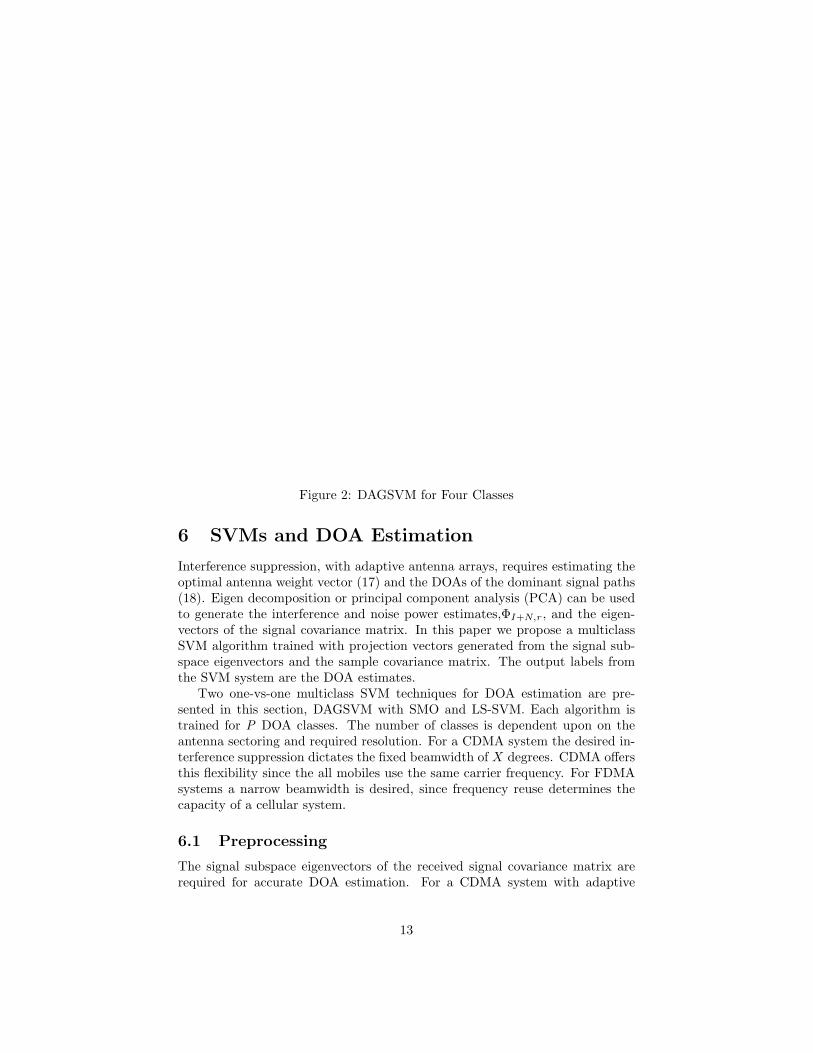
The DAGSVM algorithm is based on the DDAG architecture with each nodecontaining a binary SVM classifier of the ith and jth classes. The training timeof the DAGSVM classifier is equivalent to the standard one-vs-one SVMs. Theperformance benefit of the DAGSVM is realized when the ith classifier is selectedat the ith/jth node and the jth class is eliminated. Thus any other class pairscontaining the jth class are removed from the remaining SVM operations andthe jth class is not a candidate for the output label. Refer to Figure 2 fora diagram of the DAGSVM approach. An analysis of the training times forone-vs-rest, one-vs-one, and the DAGSVM with SMO are presented in [22].

12

Figure 2: DAGSVM for Four Classes

6 SVMs and DOA Estimation

Interference suppression, with adaptive antenna arrays, requires estimating theoptimal antenna weight vector (17) and the DOAs of the dominant signal paths(18). Eigen decomposition or principal component analysis (PCA) can be usedto generate the interference and noise power estimates,ΦI+N,r , and the eigen-vectors of the signal covariance matrix. In this paper we propose a multiclassSVM algorithm trained with projection vectors generated from the signal sub-space eigenvectors and the sample covariance matrix. The output labels fromthe SVM system are the DOA estimates.

Two one-vs-one multiclass SVM techniques for DOA estimation are pre-sented in this section, DAGSVM with SMO and LS-SVM. Each algorithm istrained for P DOA classes. The number of classes is dependent upon on theantenna sectoring and required resolution. For a CDMA system the desired in-terference suppression dictates the fixed beamwidth of X degrees. CDMA offersthis flexibility since the all mobiles use the same carrier frequency. For FDMAsystems a narrow beamwidth is desired, since frequency reuse determines thecapacity of a cellular system.

6.1 Preprocessing

The signal subspace eigenvectors of the received signal covariance matrix arerequired for accurate DOA estimation. For a CDMA system with adaptive

13

antenna arrays, refer to Section 3.0.2, the covariance matrix of the receivedsignal is

Rrr = E[xrxH

r

], (58)

where xr ε Cn is a complex random vector process.In our machine learning based DOA estimation algorithm the principal eigen-

vectors must be calculated. Eigen decomposition (ED) is the standard compu-tational approach for calculating the eigenvalues and eigenvectors of a the co-variance matrix. ED is a computationally intense technique, faster algorithms,such as PASTd [23] with 4NL+O(L) computations, have been developed for realtime processing applications; L is the dimension of the desired signal subspaceand N is the dimension of the input vector.

For a machine learning based approach to DOA estimation the output of theRake receiver is used to calculate the sample covariance matrix Rrr,

Rrr =1M

K∑

k=K−M+1

xr (k)xHr (k) (59)

The dimension of the observation matrix is D × M and the dimension of thesample covariance matrix is D×D . D is the number of antenna elements and Mis ideal sample size (window length) which must be determined through testing.

6.1.1 Algorithms for DOA Estimation

Two primary, classic methods for subspace based DOA estimation exist in lit-erature, Multiple Signal Classification (MUSIC) [24] and Estimation of SignalParameters Via Rotational Invariance Techniques (ESPRIT) [25]. The MUSICalgorithm is based on the noise subspace and ESPRIT is based on the signal sub-space. There are implementation issues involved with each approach; accuratearray characterization is required for MUSIC and multiple eigen decompositionsare required for ESPRIT.

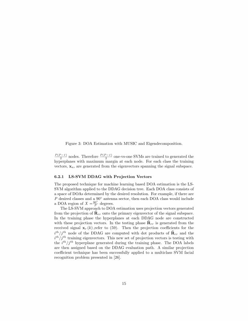
Figure 3 includes a plot showing DOA estimation results with the MUSICalgorithm. DOA estimates for ten subspace updates are plotted. The antennaarray consists of eight elements and the input signal contains one distinct sig-nals with a DOA at 25. These results serve as a benchmark for the machinelearning based DOA estimation. For the proposed machine learning techniquethere is a trade-off between the accuracy of the DOA estimation and antennaarray beamwidth. An increase in DOA estimation accuracy translates into asmaller beamwidth and a reduction in MAI. Therefore the accuracy in DOAestimation directly influences the minimum required power transmitted by themobile. There should be a balance between computing effort and reduction inMAI.

6.2 Support Vectors for Multiclassification of DOAs

The multiclass SVM implemented with a DDAG is the primary technique pre-sented for DOA estimation. The DDAG tree is initialized for P classes with

14

Figure 3: DOA Estimation with MUSIC and Eigendecomposition.

P(P−1)2 nodes. Therefore P(P−1)

2 one-vs-one SVMs are trained to generated thehyperplanes with maximum margin at each node. For each class the trainingvectors, xn, are generated from the eigenvectors spanning the signal subspace.

6.2.1 LS-SVM DDAG with Projection Vectors

The proposed technique for machine learning based DOA estimation is the LS-SVM algorithm applied to the DDAG decision tree. Each DOA class consists ofa space of DOAs determined by the desired resolution. For example, if there areP desired classes and a 90 antenna sector, then each DOA class would includea DOA region of X = 90

P degrees.The LS-SVM approach to DOA estimation uses projection vectors generated

from the projection of Rrr onto the primary eigenvector of the signal subspace.In the training phase the hyperplanes at each DDAG node are constructedwith these projection vectors. In the testing phase Rrr is generated from thereceived signal xr (k) ,refer to (59). Then the projection coefficients for theith/jth node of the DDAG are computed with dot products of Rrr and theith/jth training eigenvectors. This new set of projection vectors is testing withthe ith/jth hyperplane generated during the training phase. The DOA labelsare then assigned based on the DDAG evaluation path. A similar projectioncoefficient technique has been successfully applied to a multiclass SVM facialrecognition problem presented in [26].

15

6.2.2 LS-SVM DDAG based DOA Estimation Algorithm

The following routine is applied to each Rake finger, if there are R fingers inthe Rake receiver, then there will be R parallel implementations.

• Preprocessing

1. Generate the D × N training signal vectors for the P SVM classes,D is the number of antenna elements, N is the number of samples.

2. Generate the P sample covariance matrices, M,with M samples fromthe D ×N data vector

3. Calculate the signal eigenvector, S, from each of the P sample co-variance matrices.

4. Calculate the D × 1 projection vectors, M× S, for each of the Pclasses. The ensemble of projection vectors consists of N

M samples

5. Store the projection vectors for the training phase and the eigenvec-tors for the testing phase.

• LS-SVM training

1. With the P projection vectors train the P(P−1)2 nodes with the one-

vs-one LS-SVM algorithm. .

2. Store the LS-SVM variables, αk and b from equation (45) , whichdefine the hyperplane separation for each DDAG node.

• LS-SVM testing for the ith/jth node DDAG node

1. Acquire D × N input signal from antenna array, this signal has anunknown DOA.

2. Generate the P sample covariance matrices with M samples from theD ×N data vector.

3. Calculate two D × 1 projection vectors with the ith and jth eigen-vectors from the preprocessing steps.

4. Test both projection vectors against the LS-SVM hyperplane for theith/jth node. This requires two separate LS-SVM testing cycles, onewith the projection vector from the ith eigenvector and one with theprojection vector from the jth eigenvector.

5. Calculate the average value of the two LS-SVM output vectors (la-bels). Select the value which is closest to the correct label, 0/1.

6. Repeat process for the next DDAG node in the evaluation path ordeclare the final DOA label.

16

6.3 Simulation Results

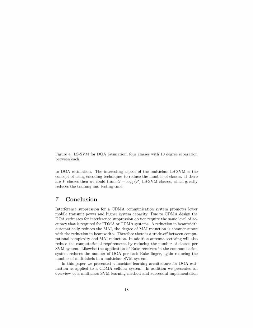
Two simulation plots are included below. Each simulation consists of a fourclass LS-SVM DDAG system. Figure 4 shows results for a ten degree range perclass. Figure 5 shows results for a one degree range per class. Testing showsthat the LS-SVM DDAG system accurately classifies the DOAs for any desirednumber of classes and DOA separations from one degree to fifteen degrees.

The antenna array includes eight elements, therefore the training and testsignals were 8×1 vectors. The training and test signals are the complex outputsfrom the antenna array. The received complex signal is modeled with a zeromean normal distribution with unit variance; the additive noise includes a zeromean distribution with a 0.2 variance. The DOAs for the set of test signals areunknown to the system. Both the training and test signals consisted of 1500samples and the window length of the sample covariance matrix was set to five.Therefore the training and test sets were composed of 300 samples of each 8× 1projection vector.

The system training consists of six DDAG nodes for the four DOA classes.To completely test the LS-SVM DDAG system’s capabilities the simulation wereautomated to test a wide range of DOAs. The DOA test set consisting of signalsranging from three degrees before the first DOA class to three degrees after thelast DOA class. Thus there were forty-six test signals for Figure 4 and fourteentest signals for Figure 5.

As can been seen from the two plots the LS-SVM DDAG DOA estimationalgorithm is extremely accurate. No misclassifications were logged. By testingtwo projection vectors at each node there is a possibility of classifying the DOAbetween two DOA labels, effectively increasing the resolution of the system.This condition exists if the average value of the two LS-SVM output vectors areequal, or within a set range. This occurs at the 10 degree point in Figure 4.

6.4 Multilabel Capability for Multiple DOAs

The machine learning algorithm must generate multiclass labels, yi ε χ, whereχ ε [−90, 90] is a set of real numbers that represent an appropriate range ofexpected DOA values, and multiple labels yi, i = 1 . . .L for L dominant signalpaths. If antenna sectoring is used in the cellular system the multiclass labelsare from the set χ ε [Si], where Si is field of view for the ith sectors.

In DOA estimation for CDMA cellular systems there can be multiple DOAsfor a given signal. This results from multipath effects induced by the envi-ronment. The Rake receiver design includes independent receivers that tracksignals within a specific time delay. This design reduces the number of DOAstracked for a given Rake receiver finger. The machine learning system must beable to discriminate between a small number of independent DOAs that includesignal components with similar time delays. With this constraint the machinelearning algorithm must be a multiclass system and able to process multiplelabels.

The multiclass LS-SVM with output encoding is another possible approach

17

Figure 4: LS-SVM for DOA estimation, four classes with 10 degree separationbetween each.

to DOA estimation. The interesting aspect of the multiclass LS-SVM is theconcept of using encoding techniques to reduce the number of classes. If thereare P classes then we could train G = log2 (P) LS-SVM classes, which greatlyreduces the training and testing time.

7 Conclusion

Interference suppression for a CDMA communication system promotes lowermobile transmit power and higher system capacity. Due to CDMA design theDOA estimates for interference suppression do not require the same level of ac-curacy that is required for FDMA or TDMA systems. A reduction in beamwidthautomatically reduces the MAI, the degree of MAI reduction is commensuratewith the reduction in beamwidth. Therefore there is a trade-off between compu-tational complexity and MAI reduction. In addition antenna sectoring will alsoreduce the computational requirements by reducing the number of classes perSVM system. Likewise the application of Rake receivers in the communicationsystem reduces the number of DOA per each Rake finger, again reducing thenumber of multilabels in a multiclass SVM system.

In this paper we presented a machine learning architecture for DOA esti-mation as applied to a CDMA cellular system. In addition we presented anoverview of a multiclass SVM learning method and successful implementation

18

Figure 5: LS-SVM for DOA estimation, four classes with 1 degree separationbetween each.

of a multiclass LS-SVM DDAG system for DOA estimation. Initial simulationresults show a high degree of accuracy, as related to the DOA classes and provethat the LS-SVM DDAG system has a wide range of performance capabilities.Future work will investigate the performance of the LS-SVM DDAG system fora multiclass, multilabel DOA estimation problem and more complex communi-cation channels will be included in the simulations.

References

[1] Joseph C. Liberti, Jr. and Theodore S. Rappaport, Smart Antennas forWireless Communications: IS-95 and Third Generation CDMA Applica-tions, Prentice Hall, Upper Saddle River, NJ, 1999.

[2] J.H. Winters, “Signal Acquisition and Tracking with Adaptive Arrays in theDigital Mobile Radio System IS-54 with Flat Fading,” IEEE Transactionson Vehicular Technology, Vol. 42, No. 4, 377-384, November 1993.

[3] Z. Raida, “Steering an Adaptive Antenna Array by the Simplified KalmanFilter,” IEEE Transactions on Antennas and Propagation, Vol. 43, No. 6,627-629, June 1995.

[4] Ahmed H. El Zooghby, Christos G. Christodoulou, and Michael Geor-giopoulos, “A Neural Network-Based Smart Antenna For Multiple Source

19

Tracking”, IEEE Transactions On Antennas and Propagation, vol. 48, no.5, pp. 768-776, May 2000

[5] Ahmed H. El Zooghby, Christos G. Christodoulou, and Michael Geor-giopoulos, “Performance of Radial-Basis Function Networks for Directionof Arrival Estimation with Antenna Arrays”, IEEE Transactions On An-tennas and Propagation, vol. 45, no. 11, pp. 1611-1617, November 1997

[6] Ahmed H. El Zooghby, Christos G. Christodoulou, and Michael Geor-giopoulos, “Neural Network-Based Adaptive Beamforming for One- andTwo- Dimensional Antenna Arrays”, IEEE Transactions On Antennas andPropagation, vol. 46, no. 12, pp. 1891-1893, December 1998

[7] Farrokh Rashid-Farrokhi, Leandros Tassiulas, K.J. Ray Liu, “Joint Opti-mum Power Control and Beamforming in Wireless Networks Using AntennaArrays”, IEEE Transactions On Communications, vol. 46, no. 10, pp. 1313-1324, October 1998.

[8] Rober A. Monzingo and Thomas W. Miller, Introduction to Adaptive An-tenna Arrays, Wiley, New York, 1980.

[9] Teong Chee Chuah, Bayan S. Sharif, and Oliver R. Hinton, “Robust Adap-tive Spread-Spectrum Receiver with Neural-Net Preprocessing in Non-Gaussian Noise”, IEEE Transactions On Neural Networks, vol. 12, no. 3,pp. 546-558, May 2001.

[10] David C. Chen and Bing J. Sheu, “A Compact Neural-Network-BasedCDMA Receiver”, IEEE Transactions On Circuits and Systems II: Ana-log and Digital Signal Processing, vol. 45, no. 3, pp. 384-387, March 1998.

[11] Kaushik Das and Salvatore D. Morgera, “Adaptive Interference Cancel-lation for DS-CDMA Systems Using Neural Network Techniques”, IEEEJournal On Selected Areas In Communications, vol. 16, no. 9, pp.1774-1784,December 1998.

[12] Xiao Ming Gao, Xiao Zhi Gao, Jarno M. A. Tanskanen, and Seppo J.Ovaska, “Power Prediction in Mobile Communication Systems Using anOptimal Neural-Network Structure”, IEEE Transactions On Neural Net-works, vol. 8, no. 6, pp. 1446-1455, November 1997.

[13] S. Chen, A.K. Samingan, and L. Hanzo, “Support Vector Machine Mul-tiuser Receiver for DS-CDMA Signals in Multipath Channels”, IEEETransactions On Neural Networks, vol. 12, no. 3, pp. 604-611, May 2001.

[14] Daniel J. Sebald and James A. Bucklew, “Support Vector Machine Tech-niques for Nonlinear Equalization”, IEEE Transactions On Signal Process-ing, vol. 48, no. 11, pp. 3217-3226, November 2000.

20

[15] Klaus-Robert Muller, Sebastion Mika, Gunnar Ratsch, Koji Tsuda, andBernard Scholkopf, “An Introduction to Kernel-Based Learning Algo-rithms”, IEEE Transactions on Neural Networks, vol. 12, no. 2, pp. 181-201,March 2001.

[16] Vladimir N. Vapnik, The Nature of Statistical Learning Theory, Springer-Verlag, New York, 1995.

[17] Nello Christianini and John Shawe-Taylor, An Introduction to Support Vec-tor Machines , Cambridge University Press, New York, 2000.

[18] Johan A.K. Suykens, “Support Vector Machines: A Nonlinear Modellingand Control Perspective”, European Journal of Control, vol 7, pp. 311-327,2001

[19] John C. Platt, “Fast Training of Support Vector Machines using SequentialMinimal Optimization”, in Advances in Kernel Methods-Support VectorLearning, B. Scholk

..opf, C.J.C. Burges, and A.J. Smola, Eds, pp 185-208,

Cambridge, MA, MIT Press, 1999.

[20] John C. Platt, “Using Analytic QP and Sparseness to Speed Training ofSupport Vector Machines”, in Advances in Neural Information ProcessingSystems, vol. 11, Cambridge, MA, MIT Press, 1999.

[21] J.A.K. Suykens, L. Lukas, P. Van Dooren, B. DeMoor, and J. Vandewalle,“Least Squares Support Vector Machine Classifiers: a Large Scale Algo-rithm”, ECCTD’99 European Conf. on Circuit Theory and Design, pp.839-842, August 1999.

[22] John C. Platt, Nello Christianini, and John Shawe-Taylor, “Large MarginDAGs for Multiclass Classification”, in Advances in Neural InformationProcessing Systems, vol. 12, pp. 547-553, Cambridge, MA, MIT Press, 2000.

[23] Bin Yang, “Projection Approximation Subspace Tracking”, IEEE Transac-tions on Signal Processing, vol. 43, no. 1, pp. 95-107, January 1995.

[24] R.O. Schmidt, “Multiple Emitter Location and Signal Parameter Estima-tion”, IEEE Transactions on Antennas and Propagation, AP-34, pp. 276-280, March 1986.

[25] Richard H. Roy, and Thomas Kailath, “ESPRIT-Estimation of Signal Pa-rameters Via Rotational Invariance Techniques”, IEEE Transactions OnAcoustics, Speech, and Signal Processing, vol. 37, no. 7, pp. 984-995, July1989.

[26] Guodong Guo, Stan Z. Li, and Kap Luk Chan, “Support Vector Machinesfor Face Recognition”, Image and Vision Computing, vol 19, pp. 631-638,2001.

21