Supporting Analysis of Dimensionality Reduction Results withContrastive Learning
Takanori Fujiwara, Oh-Hyun Kwon, and Kwan-Liu Ma
Abstract— Dimensionality reduction (DR) is frequently used for analyzing and visualizing high-dimensional data as it provides agood first glance of the data. However, to interpret the DR result for gaining useful insights from the data, it would take additionalanalysis effort such as identifying clusters and understanding their characteristics. While there are many automatic methods (e.g.,density-based clustering methods) to identify clusters, effective methods for understanding a cluster’s characteristics are still lacking. Acluster can be mostly characterized by its distribution of feature values. Reviewing the original feature values is not a straightforwardtask when the number of features is large. To address this challenge, we present a visual analytics method that effectively highlightsthe essential features of a cluster in a DR result. To extract the essential features, we introduce an enhanced usage of contrastiveprincipal component analysis (cPCA). Our method, called ccPCA (contrasting clusters in PCA), can calculate each feature’s relativecontribution to the contrast between one cluster and other clusters. With ccPCA, we have created an interactive system including ascalable visualization of clusters’ feature contributions. We demonstrate the effectiveness of our method and system with case studiesusing several publicly available datasets.
Index Terms—Dimensionality reduction, contrastive learning, principal component analysis, high-dimensional data, visual analytics
1 INTRODUCTION
High-dimensional data visualization is one of the major research top-ics in the visualization community [46, 47]. Various types of visual-ization methods (e.g., the parallel coordinates [33], scatterplot matri-ces [27], and star coordinates [38]) have been introduced to presenthigh-dimensional information in a space [47] (typically 2D on a com-puter screen) that human viewers can perceive and interpret. Amongthese methods, dimensionality reduction (DR) methods are suitable toprovide an overview of the relationships across the high-dimensionaldata points [47, 54, 61].
The strength of DR methods is their capability of uncovering thesimilarity between data points as spatial proximity [75]. In DR results,by referring to the “similarity ≈ proximity” [75] relationship, we canintuitively find useful patterns, such as clusters and outliers. Manyfields of study, including biology [31], social science [68], and machinelearning [58], require analyzing high-dimensional data and thus rely onDR methods.
According to the recent surveys [12, 54], analyzing a DR resultinvolves the following tasks: (1) identifying clusters in the DR result, (2)understanding the characteristics of the clusters, and (3) comparing theclusters with predefined classes of data points [12, 54]. In the case thatthe DR result has interpretable axes, such as the dimensions generatedby principal components analysis (PCA) [32, 37], understanding thecharacteristics of each axis and comparing the axis with the originaldimensions (or features) are also included as part of the analysis tasks.
Among the aforementioned tasks, the main task sequence is firstidentifying clusters and then understanding their characteristics [12].While many automatic methods (e.g., density-based clustering meth-ods [8, 15, 22, 40]) have been introduced to identify clusters (the firsttask), methods to assist the second task have still not been well stud-ied, especially in the case that the data has many features. Reviewingthe original feature values is essential to understanding each cluster’scharacteristics. To support this task, many existing visual analyticssystems [18, 42, 48, 56, 63] employ basic statistical plots, such as his-tograms and parallel coordinates, for inspecting each feature of theselected clusters. However, because these visualizations render all ofthe features’ values, they are limited in handling a large number offeatures. In addition, even if we were able to show all the features,
• Takanori Fujiwara, Oh-Hyun Kwon, and Kwan-Liu Ma are with Universityof California, Davis. E-mail: {tfujiwara, kw, klma}@ucdavis.edu
it could be very time-consuming to find the common patterns withineach cluster or find the differences among the clusters by individuallyreferring to the values for each of the many associated features.
To address these problems, we have developed an analysis methodthat highlights those essential features for understanding characteristicsof each cluster in a DR result. For our method, we adopt contrastivelearning [77], a new emerging analysis approach for high-dimensionaldata. Contrastive learning aims to discover “patterns that are specificto, or enriched in, one dataset relative to another” [4]. Among thecontrastive learning methods, we specifically choose contrastive prin-cipal component analysis (cPCA) [4, 5, 25] and enhance it for visualanalysis. Our usage of cPCA, which we call ccPCA (contrasting clus-ters in PCA), can measure each feature’s relative contribution to eachcluster’s contrast to the others. By referring to these relative contri-butions, users can easily focus on the features they should review indetail. We describe the strengths of using ccPCA with both numericalformulas and concrete examples. In addition, because cPCA requiresparameter tuning to obtain a useful result, we develop an automaticselection method that finds the best parameter value.
Moreover, we introduce a heatmap-based visualization showing allthe features’ contributions of each cluster. By employing hierarchicalclustering and matrix reordering, our visualization helps the user findwhere clusters have similar features’ contributions or how the featureshave similar contributions within or across clusters. Additionally, withthese methods, we are able to provide a scalable visualization that canhandle the case of analyzing many features (e.g., 100 features or more).We have built an interactive visual analytics system using ccPCA and aheatmap-based visualization. We demonstrate the effectiveness of ourmethods and system with case studies using several publicly availabledatasets.
2 RELATED WORK
We survey the relevant works in (1) visualization for exploring DRresults and (2) discriminant analysis and contrastive learning.
2.1 Visualization for Exploring DR ResultsVarious visualizations have been developed to assist analysis tasks for aDR result [20,39,43,44,46,47]. Here, we focus on describing the worksthat supports the aforementioned main task sequence (i.e., identifyingclusters and understanding clusters’ characteristics). Stahnke et al. [63]developed visualizations to help understand multidimensional-scaling(MDS) [67] results. To support a feature comparison of clusters inthe MDS result, their visualization allows the user to manually selectclusters and then it depicts the selected clusters’ density plots for each ofthe features. Similarly, for a cluster comparison in the DR results, other
works [18, 42, 48, 56] visualized statistical charts (e.g., bar charts andboxplots) of the features for each manually or automatically selectedcluster. However, because the approaches in [18, 42, 48, 56, 63] depictthe statistical chart for each feature, they are not scalable when there is alarge number of features (e.g., 10 features). Broeksema et al. [14] tookfurther steps to provide a summary of the DR results. They developedvisualizations to help understand patterns that appeared in multiplecorrespondence analysis (MCA) [3], which is a similar DR methodas PCA for categorical data. They visualized each data point’s salientfeature value extracted with MCA as a colored Voronoi cell aroundeach projected point in the MCA result. This linking of the DR resultand the salient features helps the user interpret the DR result. Similarly,Joia et al. [36] linked the DR result and the information of features intoone plot. In addition to an automatic selection of clusters, they obtainedrepresentative features for each cluster by using PCA. Afterward, theyvisualized these features’ names as a word cloud within each clusteredregion instead of showing the projected points. Turkay et al. [69] alsoused PCA to obtain the representative features in the MDS result.
Among the mentioned studies, the works by Joia et al. [36] andTurkay et al. [69] are most related to ours in terms of identifying therepresentative features for each cluster. To identify such features, bothmethods refer to each cluster’s principal components (PCs) computedby PCA (and the correlation between the features and PCs). Eventhough they applied PCA within each cluster, the computed PCs mightcapture only the global tendency in the dataset. For example, all clustersmay have similar or even the same PCs. Also, their methods cannotfind features that highly contribute to the differentiation or contrastbetween one cluster and the others. It is important to provide featuresthat make each cluster’s characteristics unique.
2.2 Discriminant Analysis and Contrastive LearningDiscriminant analysis, including linear discriminant analysis (LDA) [34],quadratic discriminant analysis (QDA) [51], and mixture discriminantanalysis (MDA) [29], is a supervised learning method used forclassification and DR. Discriminant analysis methods use labeleddata points as a learning set and construct a classifier to distinguisheach class as much as possible [34]. For example, LDA finds newdimensions (or components) which provide good separations betweeneach class. Note that while both PCA and LDA can be categorizedas linear DR methods, PCA is an unsupervised method and findsdimensions which maximize the variance of the input data points.
As similar to PCA, we can obtain the contribution of each origi-nal dimension (or feature) to each component constructed by LDA.Therefore, for visual analytics, LDA has been utilized to inform thefeatures which have an important role to distinguish clusters. For exam-ple, Wang et al. [72] developed linear discriminative star coordinates(LDSC). LDSC shows each feature’s contribution to distinguishinga cluster from each other as a length of a corresponding axis of thestar coordinates [38]. To obtain a better-clustered result, the user canuse these axes as interfaces to discard the less contributed features orchange the weight of the features used for clustering.
While discriminant analysis is used for discriminating the data pointsbased on their classes, contrastive learning [77] focuses on findingpatterns which contrast one dataset with another [4]. For example,contrastive PCA (cPCA) [4, 5, 25] is the extended version of PCA forcontrastive learning. cPCA takes two different datasets (i.e., target andbackground), and then identifies the directions (or contrastive principalcomponents) that have a higher variance in the target dataset whencompared to the background dataset. Projection of the target datasetwith these contrastive principal components provides the patterns whichare uniquely found only in the target dataset. In addition to cPCA,several extended methods for contrastive learning have been developed(e.g., contrastive versions of latent Dirichlet allocation [77], hiddenMarkov models [77], regressions [25], multivariate singular spectrumanalysis [19], and variational autoencoders [6]).
To the best of our knowledge, this paper is the first research using acontrastive learning method, specifically cPCA, for interactive visualanalytics. We demonstrate the major advantages of using cPCA insteadof PCA or LDA in Sect. 4.
Fig. 1: The analysis workflow.
3 WORKFLOW AND AN ANALYSIS EXAMPLE
We first define a workflow for analyzing high dimensional data usingDR, and then provide an analysis example to motivate our work.
3.1 Analysis WorkflowFig. 1 shows an analysis workflow using our method. It starts from(a) applying a DR method (e.g., MDS, PCA, or t-SNE [71]) on high-dimensional data. Then, the task is (b) to identify clusters in theDR result by applying a clustering method (e.g., k-means [28], DB-SCAN [22], or spectral clustering [53]) or selecting clusters manually.Afterward, the task is to understand the clusters’ characteristics. Thistask has two steps. The first step is (c) finding features (or dimensions)which have a high contribution to contrasting each cluster with theothers. For this step, we utilize cPCA [4, 5, 25], as described in Sect. 4.The second step is (d) reviewing the detailed differences of values ofthe highly contributed features between each corresponding cluster andthe other data points. We use existing methods for DR and clusteringwhile we introduce new methods for the last two steps. With the lasttwo steps, we can obtain an understanding of which and how featurescontribute to the uniqueness of each cluster. After understanding theselected clusters’ characteristics, as indicated with the arrows from(d) to (a) and (b), the user can update the DR result or clusters byselecting a subset of the data points based on his/her interest, changingthe parameters of the algorithms, etc.
3.2 An Analysis ExampleWe analyze the Wine Recognition dataset from UCI Machine LearningRepository [21] while following the workflow shown in Fig. 1. Thedataset includes 178 data points (wines) with 13 features (e.g., alcohol,color intensity, and flavanoids). First, to generate a DR result, we uset-SNE [71] for all of the data points. Then, to detect clusters, we applyDBSCAN [22] to the DR result. As shown in Fig. 2a, we identify threeclusters, colored with green, orange, and brown. The black data pointsare outliers or noise points labeled by DBSCAN. To understand thecharacteristics of the wines in each cluster, the system immediatelyapplies our cPCA-based analysis method for each detected cluster.Now, we have obtained the features’ contributions to contrasting eachcluster. The measures of contributions are visualized with a blue-to-reddivergent colormap, as indicated in Fig. 2b. As the absolute valueof the measure approaches 1, the corresponding feature has a highercontribution. Finally, for each cluster, we visualize histograms of valuesof the three features that have the highest contributions. The results areshown in Fig. 2c. The histograms for each target cluster are coloredwith its respective cluster color, while the others are colored gray. They-axis shows relative frequency and its maximum limit is set to themaximum relative frequency of each pair of the histograms.
Based on the result shown in Fig. 2, we can easily perceive each clus-ter’s characteristics. For example, the green cluster has higher alcoholpercentage (‘Alc’) and flavanoids when compared to the others. Theorange cluster has lower magnesium, proline, and alcohol percentage.Also, the brown cluster has lower OD280/OD315 (i.e., low dilutiondegree), lower hue, and higher color intensity. The black outliers havehigher magnesium and proanthocyanidins (‘Proanth’).
Even though this analysis example uses relatively a small number offeatures and clusters, finding these results is not a trivial task withoutthe suggestions of highly contributed features. For example, in Fig. 3,similar to [42], we visualize each cluster’s feature values with parallelcoordinates [33]. Without our method, to find the same results, theuser would need to review all the features of each cluster one by one.This is not only time-consuming but also introduces a possibility ofoverlooking important characteristics.
2
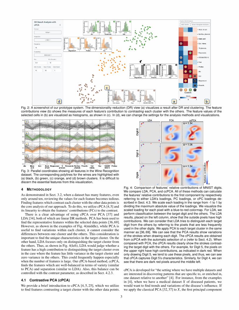
Fig. 2: A screenshot of our prototype system. The dimensionality reduction (DR) view (a) visualizes a result after DR and clustering. The featurecontributions view (b) shows the measures of each feature’s contribution to contrasting each cluster with the others. The feature values of theselected cells in (b) are visualized as histograms, as shown in (c). In (d), we can change the settings for the analysis methods and visualizations.
Fig. 3: Parallel coordinates showing all features in the Wine Recognitiondataset. The corresponding polylines for the wines are highlighted with(a) black, (b) green, (c) orange, and (d) brown clusters. It is difficult todiscern the essential features from this visualization.
4 METHODOLOGY
As demonstrated in Sect. 3.2, when a dataset has many features, evenonly around ten, reviewing the values for each feature becomes tedious.Finding features which contrast each cluster with the other data points isthe core analysis of our approach. To do this, we utilize cPCA [4,5] andits linearity to obtain the features’ contributions (FCs) to the contrast.
There is a clear advantage of using cPCA over PCA [37] andLDA [34], both of which are linear DR methods. PCA has been used tofind the representative features within the selected data points [36, 69].However, as shown in the examples of Fig. 4(middle), while PCA isuseful to find variations within each cluster, it cannot consider thedifferences between one cluster and the others. This consideration isimportant to find the unique characteristics in the target cluster. On theother hand, LDA focuses only on distinguishing the target cluster fromthe others. Thus, as shown in Fig. 4(left), LDA would judge whether afeature has a high contribution to distinguishing the target cluster evenin the case where the feature has little variance in the target cluster andzero variance in the others. This could frequently happen especiallywhen the number of features is large. Our cPCA-based method, ccPCA,finds the features which are well-balanced in terms of variety (similarto PCA) and separation (similar to LDA). Also, this balance can becontrolled with the contrast parameter, as described in Sect. 4.2.3.
4.1 Contrastive PCA (cPCA)We provide a brief introduction to cPCA [4, 5, 25], which we utilizeto find features contrasting a target cluster with the other data points.
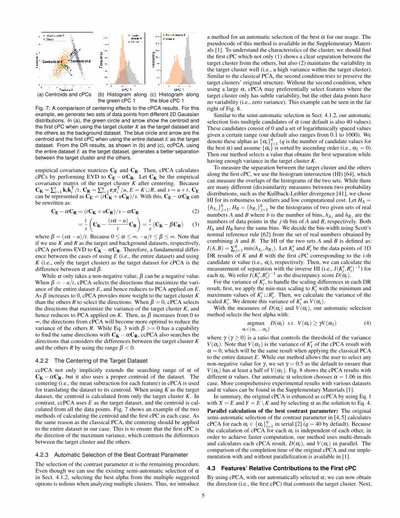
Fig. 4: Comparison of features’ relative contributions of MNIST digits.We compare LDA, PCA, and ccPCA. All of these methods can calculatethe features’ relative contributions to the first component by respectivelyreferring to either LDA’s loadings, PC loadings, or cPC loadings de-scribed in Sect. 4.3. We scale each loading in the range from -1 to 1 bydividing the maximum absolute value of the loadings. We visualize thescaled loading for each pixel with a blue-to-red colormap. For LDA, weperform classification between the target digit and the others. The LDAresults, placed on the left column, show that the outside pixels have highcontributions. We can consider that LDA tries to distinguish each targetdigit from the others by referring to the pixels that are less frequentlyused in the other digits. We apply PCA to each target cluster in the samemanner as [36, 69]. We can see that the PCA results show variationsof the strokes when drawing each digit. The cPCA results are obtainedfrom ccPCA with the automatic selection of α (refer to Sect. 4.2). Whencompared with PCA, the cPCA results clearly show the strokes contrast-ing the target digit with the others. For example, for Digit 5, the pixels onthe upper right have high contributions, as indicated in dark red. Whenonly drawing Digit 5, we tend to use these pixels, and thus, we can seethat cPCA captures Digit 5’s characteristics. Similarly, for Digit 4, we cansee that there are dark red pixels around the middle left.
cPCA is developed for “the setting where we have multiple datasets andare interested in discovering patterns that are specific to, or enriched in,one dataset relative to another” [4]. For instance, from the examplesin [4], when we have a medical dataset X of diseased patients, wewould want to find trends and variations of the disease’s influence. Ifwe apply the classical PCA [32, 37] to X , the first principal component
3
Fig. 5: cPCA results of the Mice Protein Expression dataset [30] from [4].A different contrast parameter α value is used for each result. Whenα = 0, cPCA generates the same result when applying PCA to the targetdataset. In this result, we cannot see clear differences between downsyndrome (DS) and non-DS mice, indicated with red and blue points,respectively. While clear differences between DS and non-DS start toappear when α = 1.7, we can see that DS is further separated into twogroups when α = 36.7. More examples can be found in [4,5].
would only present the diseased patients’ demographic variations [24],instead of showing the variation of the disease’s effects. However, ifthere is another medical dataset Y of healthy patients, cPCA can utilizethe fact that Y could have similar demographic variations as X , andno variations related to the disease. By taking X and Y as the targetand background datasets, respectively, cPCA can find the directions (orcomponents) in which X has high variance but Y has low variance.
4.1.1 Description of the AlgorithmNow, we describe how cPCA obtains such directions by using thetarget and background datasets. Let X = {xi}n
i=1 be the target datasetand Y = {yi}m
i=1 be the background dataset where xi,yi ∈ Rd , n andm are the numbers of data points, and d is the number of dimensions(or features). Similar to the classical PCA, for the first step, cPCAapplies centering to each dimension of X and Y and then obtains theircorresponding empirical covariance matrices CX and CY. Let v be anyunit vector of d dimensions.
Then, with a given direction v, the variances for the target and back-ground datasets can be written as: λX (v)
def= vTCXv, λY (v)
def= vTCYv.
Now, the optimization that finds a direction v∗ where X has high vari-ance but Y has low variance can be written as:
v∗ = argmaxv
λX (v)−αλY (v) = argmaxv
vT(CX−αCY)v (1)
where α is a contrast parameter (0≤α ≤∞). We describe the details ofα in Sect. 4.1.2. From Eq. 1, we can see that v∗ corresponds to the firsteigenvector of the matrix C def
= (CX−αCY). The eigenvectors of C canbe calculated with eigenvalue decomposition (EVD). These computedeigenvectors are called contrastive principal components (cPCs) andare orthogonal to each other. Similar to the classical PCA, by usingthese cPCs (typically two cPCs), we can plot the DR result of X . Anexample from [4] is shown in Fig. 5.
4.1.2 The Contrast Parameter and Semi-Automatic SelectionThe contrast parameter α controls the trade-off between having hightarget variance and low background variance. When α = 0, cPCs willonly maximize the variance of the target dataset. These cPCs are thesame as the principal components (PCs) of the target dataset whencomputed with the classical PCA. As α increases, cPCs will becomemore optimal directions that reduces the variance of the backgrounddataset. Fig. 5 shows the example from [4] with different α values.
As shown in Fig. 5, the selection of α has a strong impact on theDR result. Thus, Abid and Zhang et al. [4, 5] introduced an algorithmsuggesting multiple α values. Their algorithm calculates a set of cPCsfor each of the multiple values of α (with 40 values as their default),and the α values are logarithmically spaced in a certain range (thedefault is between 0.1 and 1000). Then, the similarity between eachpair of the different cPCs, each obtained with a different α value, ismeasured by calculating the product of the cosine of the principalangles. Afterward, based on the user’s input p (the number of values ofα to suggest), the algorithm finds p clusters from the similarities withspectral clustering [53]. Finally, the algorithm returns p values of α
which correspond to the medoids of the clusters. From the suggested p
(a) PCA (b) cPCA (α = 2.15) (c) ccPCA (α = 4.38)Fig. 6: The DR results of the Wine Recognition dataset. The clusterlabels generated in Sect. 3.2 are used. Here, we try to find the (c)PCcontrasting the green cluster. In (a), we apply the classical PCA to theentire dataset. Though there is a separation of the green cluster whenusing the first and second PCs, there are overlaps of the green andorange clusters when only using the first PC (PC 1). In (b), the datapoints in the green cluster are used as the target dataset and the otherdata points are used as the background dataset. α value is selectedfrom the suggestions using the semi-automatic selection in Sect. 4.1.2.We cannot see a clear separation of the green cluster from the others. In(c), we use the entire data points instead of only the green cluster as thetarget dataset. α value is selected with our automatic selection methodin Sect. 4.2.3. We can see a better separation when compared to that of(a) and (b) even when using only the first cPC (cPC 1).
values, the algorithm returns a set of DR results. By referring to thisset, the user can choose their preferred α value.
4.2 Finding the Direction that Contrasts a Target ClusterAs described above, cPCA discovers patterns that are specific to, orenriched in, the target dataset relative to the background dataset. In[4, 5], cPCA is designed for the situation where the patterns the userwants to identify are included within the target dataset X , while thebackground dataset Y contains the structure the user wants to removefrom the target dataset. Therefore, in [4, 5], the provided examples for{X , Y} are {‘diseased subjects’, ‘control group subjects’}, {‘patientsafter treatment’, ‘patients before treatment’}, {‘images mixed withinterests and noises’, ‘images only including noises’}, etc.
In our case, we want to find the directions (i.e., cPCs) which contrastone cluster with the other data points. If we follow the examples ofX and Y as stated above, X can be the target cluster and Y can be theother data points. However, in this case, cPCA will find cPCs that onlyenrich the variations specific to the target cluster. For example, whenthe target cluster includes diseased subjects and the other data pointscorrespond to healthy subjects, cPCA will find enriched variationswithin the diseased subjects (e.g., differences among multiple diseases),but will not consider the differences between diseased and healthysubjects.
To utilize cPCA for finding the directions contrasting a target clusterwith the others, we introduce a novel usage of cPCA, named ccPCA.Instead of using the target cluster as the target dataset X and the otherdata points as the background dataset Y , we use the entire dataset as Xand the data points other than the target cluster as Y . With this approach,we can find the directions that contrast the target cluster. As we describein the following subsections, ccPCA has the strengths in regards to twoaspects: (1) an implicit extension of the contrast parameter α and (2) aproper setting of the centroid. The DR results shown in Fig. 6 providea comparison of the classical PCA, original usage of cPCA (i.e., usingonly the target dataset as X), and ccPCA.
Let E = {ei}si=1 be the entire dataset and K = {ki}ti=1 be the target
cluster (K ⊂ E, ei,ki ∈ Rd , s and t are the numbers of data points).Then, we denote R = {ri}u
i=1 as the difference of the two sets K andE (i.e., R = E \K and u = s− t). With these notations, we can saythat ccPCA uses E and R as the target X and background Y datasets,respectively.
4.2.1 An Implicit Extension of the Contrast ParameterTo provide a simple and clear explanation, we assume the centeringeffects to the datasets E, K, and R are all the same (i.e., E, K, and R havethe same mean value for each feature). After centering the target datasetE and the background dataset R, cPCA obtains their corresponding
4
(a) Centroids and cPCs (b) Histogram alongthe green cPC 1
(c) Histogram alongthe blue cPC 1
Fig. 7: A comparison of centering effects to the cPCA results. For thisexample, we generate two sets of data points from different 2D Gaussiandistributions. In (a), the green circle and arrow show the centroid andthe first cPC when using the target cluster K as the target dataset andthe others as the background dataset. The blue circle and arrow are thecentroid and the first cPC when using the entire dataset E as the targetdataset. From the DR results, as shown in (b) and (c), ccPCA, usingthe entire dataset E as the target dataset, generates a better separationbetween the target cluster and the others.
empirical covariance matrices CE and CR. Then, cPCA calculatescPCs by performing EVD to CE−αCR. Let CK be the empiricalcovariance matrix of the target cluster K after centering. BecauseCK = ∑
ti=1 kikT
i /t, CR = ∑ui=1 rirTi /u, E = KtR, and s = u+ t, CE
can be represented as CE = (tCK +uCR)/s. With this, CE−αCR canbe rewritten as:
CE−αCR = (tCK +uCR)/s−αCR (2)
=ts
(CK−
(sα−u)t
CR
)=
ts(CK−βCR) (3)
where β = (sα−u)/t. Because 0≤ α ≤ ∞, −u/t ≤ β ≤ ∞. Note thatif we use K and R as the target and background datasets, respectively,cPCA performs EVD to CK−αCR. Therefore, a fundamental differ-ence between the cases of using E (i.e., the entire dataset) and usingK (i.e., only the target cluster) as the target dataset for cPCA is thedifference between α and β .
While α only takes a non-negative value, β can be a negative value.When β =−u/t, cPCA selects the directions that maximize the vari-ance of the entire dataset E, and hence reduces to PCA applied on E.As β increases to 0, cPCA provides more weight to the target cluster Kthan the others R to select the directions. When β = 0, cPCA selectsthe directions that maximize the variance of the target cluster K, andhence reduces to PCA applied on K. Then, as β increases from 0 to∞, the directions from cPCA will become more optimal to reduce thevariance of the others R. While Eq. 3 with β >= 0 has a capabilityto find the same directions with CK−αCR, ccPCA also searches thedirections that considers the differences between the target cluster Kand the others R by using the range β < 0.
4.2.2 The Centering of the Target Dataset
ccPCA not only implicitly extends the searching range of α ofCK−αCR, but it also uses a proper centroid of the dataset. Thecentering (i.e., the mean subtraction for each feature) in cPCA is usedfor translating the dataset to its centroid. When using K as the targetdataset, the centroid is calculated from only the target cluster K. Incontrast, ccPCA uses E as the target dataset, and the centroid is cal-culated from all the data points. Fig. 7 shows an example of the twomethods of calculating the centroid and the first cPC in each case. Asthe same reason as the classical PCA, the centering should be appliedto the entire dataset in our case. This is to ensure that the first cPC isthe direction of the maximum variance, which contrasts the differencesbetween the target cluster and the others.
4.2.3 Automatic Selection of the Best Contrast Parameter
The selection of the contrast parameter α is the remaining procedure.Even though we can use the existing semi-automatic selection of α
in Sect. 4.1.2, selecting the best alpha from the multiple suggestedoptions is tedious when analyzing multiple clusters. Thus, we introduce
a method for an automatic selection of the best α for our usage. Thepseudocode of this method is available in the Supplementary Materi-als [1]. To understand the characteristics of the cluster, we should findthe first cPC which not only (1) shows a clear separation between thetarget cluster from the others, but also (2) maintains the variability inthe target cluster well (i.e., a high variance within the target cluster).Similar to the classical PCA, the second condition tries to preserve thetarget clusters’ original structure. Without the second condition, whenusing a large α , cPCA may preferentially select features where thetarget cluster only has subtle variability, but the other data points haveno variability (i.e., zero variance). This example can be seen in the farright of Fig. 8.
Similar to the semi-automatic selection in Sect. 4.1.2, our automaticselection lists multiple candidates of α (our default is also 40 values).These candidates consist of 0 and a set of logarithmically spaced valuesgiven a certain range (our default also ranges from 0.1 to 1000). Wedenote these alphas as {αi}q
i=1 (q is the number of candidate values forthe best α) and assume {αi} is sorted by ascending order (i.e., α1 = 0).Then our method selects a value that obtains the best separation whilehaving enough variance in the target cluster K.
To measure the separation between the target cluster and the othersalong the first cPC, we use the histogram intersection (HI) [64], whichcan measure the overlaps of the histograms of the two sets. While thereare many different (dis)similarity measures between two probabilitydistributions, such as the Kullback-Leibler divergence [41], we choseHI for its robustness to outliers and low computational cost. Let HA ={hA j}b
j=1, HB = {hB j}bj=1 be the histograms of two given sets of real
numbers A and B where b is the number of bins, hA j and hB j are thenumbers of data points in the j-th bin of A and B, respectively. BothHA and HB have the same bins. We decide the bin-width using Scott’snormal reference rule [62] from the set of real numbers obtained bycombining A and B. The HI of the two sets A and B is defined as:I(A,B) = ∑
bj=1 min(hA j,hB j). Let K′i and R′i be the data points of 1D
DR results of K and R with the first cPC corresponding to the i-thcandidate α value (i.e., αi), respectively. Then, we can calculate themeasurement of separation with the inverse HI (i.e., I(K′i ,R
′i)−1) for
each αi. We refer I(K′i ,R′i)−1 as the discrepancy score D(αi).
For the variance of K′i , to handle the scaling differences in each DRresult, first, we apply the min-max scaling to K′i with the minimum andmaximum values of K′i tR′i. Then, we calculate the variance of thescaled K′i . We denote this variance of K′i as V (αi).
With the measures of D(αi) and V (αi), our automatic selectionmethod selects the best alpha with:
argmaxαi∈{α1,...,αq}
D(αi) s.t. V (αi)≥ γV (α1) (4)
where γ (γ ≥ 0) is a ratio that controls the threshold of the varianceV (αi). Note that V (α1) is the variance of K′1 of the cPCA result withα = 0, which will be the same result when applying the classical PCAto the entire dataset E. While our method allows the user to select anynon-negative value for γ , we set γ = 0.5 as the default to ensure thatV (αi) has at least a half of V (α1). Fig. 8 shows the cPCA results withdifferent α values. Our automatic α selection chooses α = 1.06 in thiscase. More comprehensive experimental results with various datasetsand α values can be found in the Supplementary Materials [1].
In summary, the original cPCA is enhanced as ccPCA by using Eq. 1with X = E and Y = E \K and by selecting α as the solution to Eq. 4.Parallel calculation of the best contrast parameter: The originalsemi-automatic selection of the contrast parameter in [4, 5] calculatescPCA for each αi ∈ {αi}q
i=1 in serial [2] (q = 40 by default). Becausethe calculation of cPCA for each αi is independent of each other, inorder to achieve faster computation, our method uses multi-threadsand calculates each cPCA result, D(αi), and V (αi) in parallel. Thecomparison of the completion time of the original cPCA and our imple-mentation with and without parallelization is available in [1].
4.3 Features’ Relative Contributions to the First cPCBy using cPCA, with our automatically selected α , we can now obtainthe direction (i.e., the first cPC) that contrasts the target cluster. Next,
5
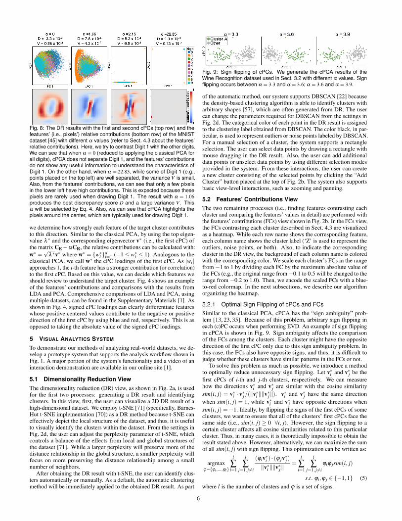
Fig. 8: The DR results with the first and second cPCs (top row) and thefeatures’ (i.e., pixels’) relative contributions (bottom row) of the MNISTdataset [45] with different α values (refer to Sect. 4.3 about the features’relative contributions). Here, we try to contrast Digit 1 with the other digits.We can see that when α = 0 (reduced to applying the classical PCA forall digits), cPCA does not separate Digit 1, and the features’ contributionsdo not show any useful information to understand the characteristics ofDigit 1. On the other hand, when α = 22.85, while some of Digit 1 (e.g.,points placed on the top left) are well separated, the variance V is small.Also, from the features’ contributions, we can see that only a few pixelsin the lower left have high contributions. This is expected because thesepixels are rarely used when drawing Digit 1. The result with α = 1.06produces the best discrepancy score D and a large variance V . Thisα will be selected by Eq. 4. Also, we can see that cPCA highlights thepixels around the center, which are typically used for drawing Digit 1.
we determine how strongly each feature of the target cluster contributesto this direction. Similar to the classical PCA, by using the top eigen-value λ ∗ and the corresponding eigenvector v∗ (i.e., the first cPC) ofthe matrix CE−αCR, the relative contributions can be calculated with:w∗ =
√λ ∗v∗ where w∗ = {w∗i }d
i=1 (−1≤ w∗i ≤ 1). Analogous to theclassical PCA, we call w∗ the cPC loadings of the first cPC. As |wi|approaches 1, the i-th feature has a stronger contribution (or correlation)to the first cPC. Based on this value, we can decide which features weshould review to understand the target cluster. Fig. 4 shows an exampleof the features’ contributions and comparisons with the results fromLDA and PCA. Comprehensive comparisons of LDA and PCA, usingmultiple datasets, can be found in the Supplementary Materials [1]. Asshown in Fig. 4, signed cPC loadings can clearly differentiate featureswhose positive centered values contribute to the negative or positivedirection of the first cPC by using blue and red, respectively. This is asopposed to taking the absolute value of the signed cPC loadings.
5 VISUAL ANALYTICS SYSTEM
To demonstrate our methods of analyzing real-world datasets, we de-velop a prototype system that supports the analysis workflow shown inFig. 1. A major portion of the system’s functionality and a video of aninteraction demonstration are available in our online site [1].
5.1 Dimensionality Reduction ViewThe dimensionality reduction (DR) view, as shown in Fig. 2a, is usedfor the first two processes: generating a DR result and identifyingclusters. In this view, first, the user can visualize a 2D DR result of ahigh-dimensional dataset. We employ t-SNE [71] (specifically, Barnes-Hut t-SNE implementation [70]) as a DR method because t-SNE caneffectively depict the local structure of the dataset, and thus, it is usefulto visually identify the clusters within the dataset. From the settings inFig. 2d, the user can adjust the perplexity parameter of t-SNE, whichcontrols a balance of the effects from local and global structures ofthe dataset [71]. While a larger perplexity will preserve more of thedistance relationship in the global structure, a smaller perplexity willfocus on more preserving the distance relationship among a smallnumber of neighbors.
After obtaining the DR result with t-SNE, the user can identify clus-ters automatically or manually. As a default, the automatic clusteringmethod will be immediately applied to the obtained DR result. As part
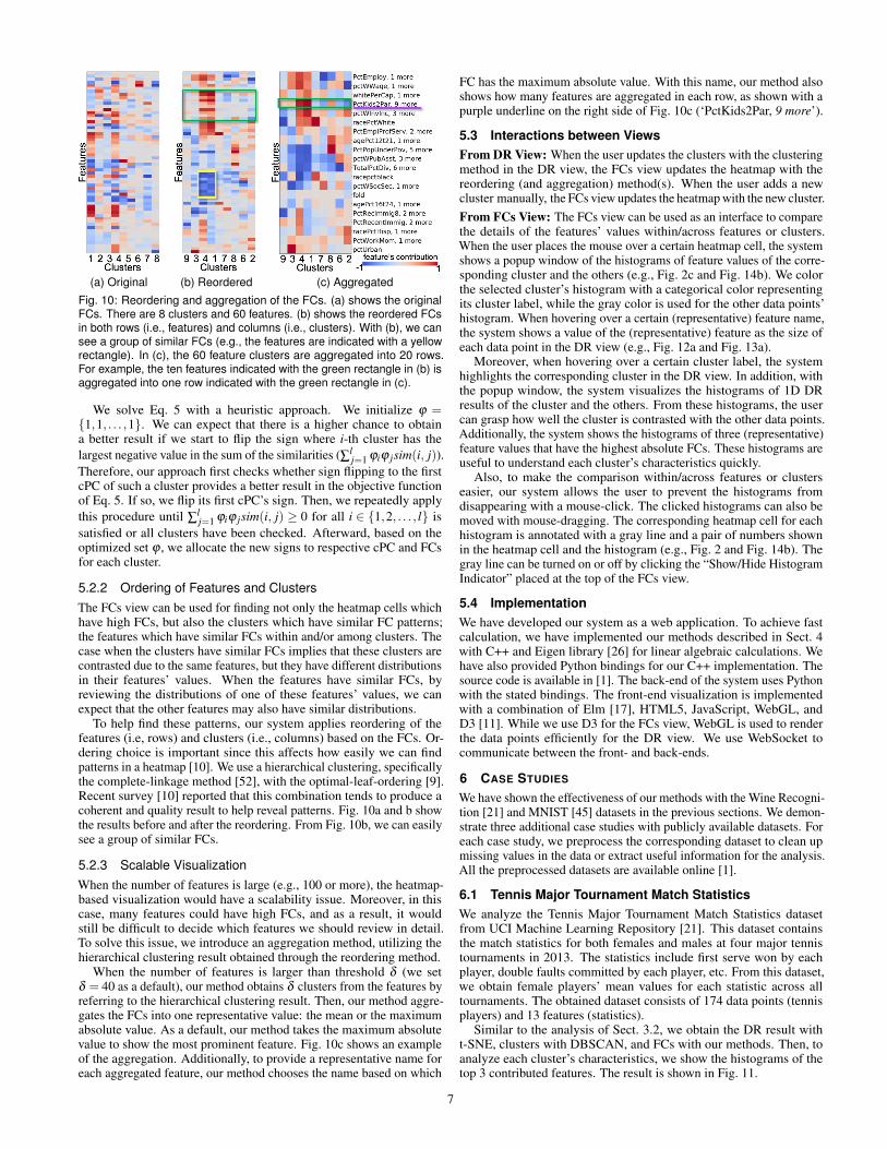
Fig. 9: Sign flipping of cPCs. We generate the cPCA results of theWine Recognition dataset used in Sect. 3.2 with different α values. Signflipping occurs between α = 3.3 and α = 3.6; α = 3.6 and α = 3.9.
of the automatic method, our system supports DBSCAN [22] becausethe density-based clustering algorithm is able to identify clusters witharbitrary shapes [57], which are often generated from DR. The usercan change the parameters required for DBSCAN from the settings inFig. 2d. The categorical color of each point in the DR result is assignedto the clustering label obtained from DBSCAN. The color black, in par-ticular, is used to represent outliers or noise points labeled by DBSCAN.For a manual selection of a cluster, the system supports a rectangleselection. The user can select data points by drawing a rectangle withmouse dragging in the DR result. Also, the user can add additionaldata points or unselect data points by using different selection modesprovided in the system. From these interactions, the user can createa new cluster consisting of the selected points by clicking the “AddCluster” button placed at the top of Fig. 2b. The system also supportsbasic view-level interactions, such as zooming and panning.
5.2 Features’ Contributions ViewThe two remaining processes (i.e., finding features contrasting eachcluster and comparing the features’ values in detail) are performed withthe features’ contributions (FCs) view shown in Fig. 2b. In the FCs view,the FCs contrasting each cluster described in Sect. 4.3 are visualizedas a heatmap. While each row name shows the corresponding feature,each column name shows the cluster label (‘Z’ is used to represent theoutliers, noise points, or both). Also, to indicate the correspondingcluster in the DR view, the background of each column name is coloredwith the corresponding color. We scale each cluster’s FCs in the rangefrom −1 to 1 by dividing each FC by the maximum absolute value ofthe FCs (e.g., the original range from−0.1 to 0.5 will be changed to therange from −0.2 to 1.0). Then, we encode the scaled FCs with a blue-to-red colormap. In the next subsections, we describe our algorithmorganizing the heatmap.
5.2.1 Optimal Sign Flipping of cPCs and FCsSimilar to the classical PCA, cPCA has the “sign ambiguity” prob-lem [13, 23, 35]. Because of this problem, arbitrary sign flipping ineach (c)PC occurs when performing EVD. An example of sign flippingin cPCA is shown in Fig. 9. Sign ambiguity affects the comparisonof the FCs among the clusters. Each cluster might have the oppositedirection of the first cPC only due to this sign ambiguity problem. Inthis case, the FCs also have opposite signs, and thus, it is difficult tojudge whether these clusters have similar patterns in the FCs or not.
To solve this problem as much as possible, we introduce a methodto optimally reduce unnecessary sign flipping. Let v∗i and v∗j be thefirst cPCs of i-th and j-th clusters, respectively. We can measurehow the directions v∗i and v∗j are similar with the cosine similaritysim(i, j) = v∗i · v∗j/(‖v∗i ‖‖v∗j‖). v∗i and v∗j have the same directionwhen sim(i, j) = 1, while v∗i and v∗j have opposite directions whensim(i, j) =−1. Ideally, by flipping the signs of the first cPCs of someclusters, we want to ensure that all of the clusters’ first cPCs face thesame side (i.e., sim(i, j) ≥ 0 ∀i, j). However, the sign flipping to acertain cluster affects all cosine similarities related to this particularcluster. Thus, in many cases, it is theoretically impossible to obtain theresult stated above. However, alternatively, we can maximize the sumof all sim(i, j) with sign flipping. This optimization can be written as:
argmaxϕ={ϕi,...,ϕl}
l
∑i=1
l
∑j=1, j 6=i
(ϕiv∗i ) · (ϕ jv∗j)‖v∗i ‖‖v∗j‖
=l
∑i=1
l
∑j=1, j 6=i
ϕiϕ jsim(i, j)
s.t. ϕi,ϕ j ∈ {−1,1} (5)where l is the number of clusters and ϕ is a set of signs.
6
(a) Original (b) Reordered (c) Aggregated
Fig. 10: Reordering and aggregation of the FCs. (a) shows the originalFCs. There are 8 clusters and 60 features. (b) shows the reordered FCsin both rows (i.e., features) and columns (i.e., clusters). With (b), we cansee a group of similar FCs (e.g., the features are indicated with a yellowrectangle). In (c), the 60 feature clusters are aggregated into 20 rows.For example, the ten features indicated with the green rectangle in (b) isaggregated into one row indicated with the green rectangle in (c).
We solve Eq. 5 with a heuristic approach. We initialize ϕ ={1,1, . . . ,1}. We can expect that there is a higher chance to obtaina better result if we start to flip the sign where i-th cluster has thelargest negative value in the sum of the similarities (∑l
j=1 ϕiϕ jsim(i, j)).Therefore, our approach first checks whether sign flipping to the firstcPC of such a cluster provides a better result in the objective functionof Eq. 5. If so, we flip its first cPC’s sign. Then, we repeatedly applythis procedure until ∑
lj=1 ϕiϕ jsim(i, j) ≥ 0 for all i ∈ {1,2, . . . , l} is
satisfied or all clusters have been checked. Afterward, based on theoptimized set ϕ , we allocate the new signs to respective cPC and FCsfor each cluster.
5.2.2 Ordering of Features and ClustersThe FCs view can be used for finding not only the heatmap cells whichhave high FCs, but also the clusters which have similar FC patterns;the features which have similar FCs within and/or among clusters. Thecase when the clusters have similar FCs implies that these clusters arecontrasted due to the same features, but they have different distributionsin their features’ values. When the features have similar FCs, byreviewing the distributions of one of these features’ values, we canexpect that the other features may also have similar distributions.
To help find these patterns, our system applies reordering of thefeatures (i.e, rows) and clusters (i.e., columns) based on the FCs. Or-dering choice is important since this affects how easily we can findpatterns in a heatmap [10]. We use a hierarchical clustering, specificallythe complete-linkage method [52], with the optimal-leaf-ordering [9].Recent survey [10] reported that this combination tends to produce acoherent and quality result to help reveal patterns. Fig. 10a and b showthe results before and after the reordering. From Fig. 10b, we can easilysee a group of similar FCs.
5.2.3 Scalable VisualizationWhen the number of features is large (e.g., 100 or more), the heatmap-based visualization would have a scalability issue. Moreover, in thiscase, many features could have high FCs, and as a result, it wouldstill be difficult to decide which features we should review in detail.To solve this issue, we introduce an aggregation method, utilizing thehierarchical clustering result obtained through the reordering method.
When the number of features is larger than threshold δ (we setδ = 40 as a default), our method obtains δ clusters from the features byreferring to the hierarchical clustering result. Then, our method aggre-gates the FCs into one representative value: the mean or the maximumabsolute value. As a default, our method takes the maximum absolutevalue to show the most prominent feature. Fig. 10c shows an exampleof the aggregation. Additionally, to provide a representative name foreach aggregated feature, our method chooses the name based on which
FC has the maximum absolute value. With this name, our method alsoshows how many features are aggregated in each row, as shown with apurple underline on the right side of Fig. 10c (‘PctKids2Par, 9 more’).
5.3 Interactions between ViewsFrom DR View: When the user updates the clusters with the clusteringmethod in the DR view, the FCs view updates the heatmap with thereordering (and aggregation) method(s). When the user adds a newcluster manually, the FCs view updates the heatmap with the new cluster.From FCs View: The FCs view can be used as an interface to comparethe details of the features’ values within/across features or clusters.When the user places the mouse over a certain heatmap cell, the systemshows a popup window of the histograms of feature values of the corre-sponding cluster and the others (e.g., Fig. 2c and Fig. 14b). We colorthe selected cluster’s histogram with a categorical color representingits cluster label, while the gray color is used for the other data points’histogram. When hovering over a certain (representative) feature name,the system shows a value of the (representative) feature as the size ofeach data point in the DR view (e.g., Fig. 12a and Fig. 13a).
Moreover, when hovering over a certain cluster label, the systemhighlights the corresponding cluster in the DR view. In addition, withthe popup window, the system visualizes the histograms of 1D DRresults of the cluster and the others. From these histograms, the usercan grasp how well the cluster is contrasted with the other data points.Additionally, the system shows the histograms of three (representative)feature values that have the highest absolute FCs. These histograms areuseful to understand each cluster’s characteristics quickly.
Also, to make the comparison within/across features or clusterseasier, our system allows the user to prevent the histograms fromdisappearing with a mouse-click. The clicked histograms can also bemoved with mouse-dragging. The corresponding heatmap cell for eachhistogram is annotated with a gray line and a pair of numbers shownin the heatmap cell and the histogram (e.g., Fig. 2 and Fig. 14b). Thegray line can be turned on or off by clicking the “Show/Hide HistogramIndicator” placed at the top of the FCs view.
5.4 ImplementationWe have developed our system as a web application. To achieve fastcalculation, we have implemented our methods described in Sect. 4with C++ and Eigen library [26] for linear algebraic calculations. Wehave also provided Python bindings for our C++ implementation. Thesource code is available in [1]. The back-end of the system uses Pythonwith the stated bindings. The front-end visualization is implementedwith a combination of Elm [17], HTML5, JavaScript, WebGL, andD3 [11]. While we use D3 for the FCs view, WebGL is used to renderthe data points efficiently for the DR view. We use WebSocket tocommunicate between the front- and back-ends.
6 CASE STUDIES
We have shown the effectiveness of our methods with the Wine Recogni-tion [21] and MNIST [45] datasets in the previous sections. We demon-strate three additional case studies with publicly available datasets. Foreach case study, we preprocess the corresponding dataset to clean upmissing values in the data or extract useful information for the analysis.All the preprocessed datasets are available online [1].
6.1 Tennis Major Tournament Match StatisticsWe analyze the Tennis Major Tournament Match Statistics datasetfrom UCI Machine Learning Repository [21]. This dataset containsthe match statistics for both females and males at four major tennistournaments in 2013. The statistics include first serve won by eachplayer, double faults committed by each player, etc. From this dataset,we obtain female players’ mean values for each statistic across alltournaments. The obtained dataset consists of 174 data points (tennisplayers) and 13 features (statistics).
Similar to the analysis of Sect. 3.2, we obtain the DR result witht-SNE, clusters with DBSCAN, and FCs with our methods. Then, toanalyze each cluster’s characteristics, we show the histograms of thetop 3 contributed features. The result is shown in Fig. 11.
7
Fig. 11: An analysis result of female players from the Tennis MajorTournament Match Statistics dataset.
Fig. 12: A result of the Nutrient dataset. (a) shows the result afterapplying t-SNE and DBSCAN. A point’s color and size show the clusteringlabel and the value of ‘calories’, respectively. (b) shows the FCs of eachcluster. (c) shows the histograms of the selected cells in (b), as indicatedwith the colored numbers in both (b) and (c).
From Fig. 11, we can see that each cluster has a different playingstyle. For example, the purple cluster tends to have low ‘DBF’ (dou-ble faults committed by player), high ‘BPC’ (break points created byplayer), and high ‘FNL’ (final number of games won by player). Thisindicates that these players had fewer mistakes in their serves and per-formed well when they were the receiver, and as a result, they wonmore games. Similarly, the orange cluster has high ‘WNR’ (winnersearned by player) and ‘NPA’ (net points attempted by player). Thesestatistics will tend to be higher when a player tries to obtain pointsaggressively during a rally. On the other hand, the brown cluster haslow ‘WNR’ but high ‘FSW’ (first serve won by player) and ‘TPW’(total points won by player). Therefore, we can say that these playerstend to obtain more points with their serves.
6.2 Food and Nutrient
We analyze the Nutrient dataset in the USDA Food CompositionDatabases [66] as an analysis example with a large number of data
Fig. 13: The result after filtering out the ‘calories’ and ‘fat’ featuresfrom the Nutrient dataset. In (a), a point size represents the value of‘carbohydrate’. The histograms of the selected cells in (b) are shown in (c).
points. We use the version available from [16]. This dataset consists ofthe nutrient content for each food. The dataset has 7,637 data points(foods) and 14 features (nutrients).
This dataset has 12,507 missing values and this is 11.7% of all thevalues. Since this high percentage of missing values could affect ananalysis result [7], we first preprocess the dataset to reduce this ratioto less than 5% [7]. We remove features where more than 40% ofthe values are missing. Also, we remove data points where more than40% of the feature values are missing. Afterward, 7,499 data pointsand 12 features remain and there are 4,447 missing values (4.9% ofall the values). We replace the missing values with the mean of eachcorresponding feature.
The result after using t-SNE, DBSCAN, and our methods is shownin Fig. 12. As shown in Fig. 12b, we can see that all clusters except forthe brown cluster have high FCs in ‘calories’, ‘fat’, or both. When com-paring the histograms of ‘calories’ and ‘fat’ for each cluster, as shownin Fig. 12c, each cluster, in fact, has different distributions in ‘calories’and ‘fat’. For example, while the yellow cluster tends to have lowcalories and fat, the orange cluster tends to have high values for both.
We have understood the main characteristics of each cluster. How-ever, the effects of the two specific features (‘calories’ and ‘fat’) are toodominant. As a result, we cannot find any other interesting patterns. Wepreprocess the dataset to filter out these two features and generate a newresult with new cluster labels, as shown in Fig. 13. At this time, fromFig. 13b, we can see that most of the clusters are contrasted by mainly‘water’, ‘carbohydrate’, or both. For example, the purple and orangeclusters placed in the upper left of Fig. 13a have fewer carbohydratesand more water when compared with the pink and green clusters, asshown in Fig. 13c. These two examples show that the FCs are useful toknow which features have a dominant effect on cluster forming in theDR result.
6.3 Communities and Crime
As an example with a large number of features, we analyze the Com-munities and Crime dataset [59] from [21]. This dataset consists ofboth socio-economic and crime statistics (e.g., the median family in-come and the number of murders) for each community. The datasetcontains 2,215 data points (communities) and 143 features (statistics)after excluding identifiers (e.g., county codes).
Because this dataset has many missing values (42,147 values, 13.3%of all the values), as similar to Sect. 6.2, we remove the features wheremore than 80% of the values are missing. The dataset now has 121
8
(a) DR result (b) Aggregated FCs and histograms
Fig. 14: The results for the Communities and Crime dataset. The topof (a) shows the result with t-SNE and DBSCAN. In the bottom of (a),the pink cluster which was not identified by DBSCAN is manually added.(b) shows 40 aggregated features from 121 features. Also, some of thehistograms of the original features are visualized at the left of (b).
features and only 963 missing values (0.4% of all the values). Wereplace the missing values with the mean of each corresponding feature.
Fig. 14a (top) shows the result after DR and clustering. As indicatedwith the purple rectangle, we manually select an additional cluster as apink cluster. Then, we obtain the FCs, as shown in Fig. 14b. Becausethere are many features, the system has aggregated them into 40 featuresusing the aggregation method described in Sect. 5.2.3. From Fig. 14b,we can say that the small clusters (yellow, purple, brown, orange, andpink) are separated from the green cluster due to race, house size, etc.—not due to the criminal statistics. For instance, as indicated with thegreen rectangles, the brown cluster has high FCs in race percentages ofAfrican Americans and Caucasians (‘racepctblack’ and ‘racePctWhite’).Also, the pink cluster has high FC in ‘PctLargHouseOccup’ (percentageof all occupied households that are large).
We show the histograms of the features aggregated to the ‘Pct-LargHouseOccup and 1 more’, as shown in the lower left of Fig. 14b.We can see that both ‘PctLargHouseOccup’ and ‘PctLargHouseFam’(percentage of family households that are large) have similar distribu-tion patterns. These patterns can be found because our aggregationmethod is performed after applying the optimal sign flipping and order-ing described in Sect. 5.2. Our aggregation method is able to provide ascalable visualization and help the user analyze many features. Anotherexample for ‘PctPopUnderPov and 3 more’ of the orange cluster isshown in the upper left of Fig. 14b. All ‘PctPopUnderPov’ (percentageof people under the poverty level), ‘agePct12t21’ (percentage of popu-lation that is 12–21), ‘agePct12t29’ (percentage of population that is12–29), and ‘MalePctNevMarr’ (percentage of males who have nevermarried) tend to have a higher value in comparison to that of others.
7 DISCUSSION AND LIMITATIONS
Generality of our method. We utilize cPCA [4, 5] to find featurescontrasting the target cluster. We discuss the reason why we use thisapproach instead of analyzing how the DR method generates clusters.If possible, the latter approach would be effective because the clusterformation is a result of the DR method. However, many of the nonlinearDR methods used for visualization (e.g., t-SNE [71], LargeVis [65],and UMAP [50]) generate irreversible low-dimensional projection of
the original data structure. These methods do not have a parametricmapping between the original and projected dimensions; therefore, itis difficult to provide information about how these DR methods affectcluster forming. Our methods provide flexibility for analyzing resultsfrom any type of DR methods.
We introduce using cPCA to understand the characteristics of theclusters identified in the DR result. Our methods can also be used inother situations. For example, even though using DR before clusteringis a common approach [74,76], our methods can support visual analyticsof clusters that are obtained from the clustering methods without goingthrough the DR step. This would be helpful to understand clusters’characteristics and to analyze the quality of the clustering methodswithout any effects derived from DR (e.g., distortion in the projectionspace). Another example is applying our methods to labeled data. Ourmethods can identify the essential features to contrast a labeled groupfrom the others. Therefore, our methods would be useful to understandthe characteristics of each group and could help design classifiers basedon the gained knowledge. Our prototype system can support these typesof analysis by changing the parts related to steps (a) and (b) in Fig. 1,such as the DR view and clustering algorithms.Advantages of using cPCA. In Sect. 4, we have already discussed theadvantages of using cPCA when compared with using PCA and LDA.It is also possible to compute the discrepancy score D introduced inSect. 4.2.3 for each original feature without using ccPCA and then usethe score as the feature contribution. However, this approach has asimilar problem with LDA because the obtained score only shows theseparation and does not take into account the variety (i.e., variance) foreach feature.
Another potential option is using the two-group differential statisticsmethods [49], such as two-sample t-test, Wilcoxon signed-rank test, andMann-Whitney U test, to find features that have differences betweenthe target cluster and the others. Unlike LDA, PCA, or cPCA, thesemethods cannot produce a quantitative measure for analyzing the FCs tothe contrast of the cluster. More importantly, these statistical methodsare designed to test whether there is a difference in a certain statistic(typically mean) between two clusters. Therefore, these methods arenot suitable for performing exploratory analysis on clusters when wedo not know their characteristics beforehand.Limitations. Since we use cPCA, we will need to address its limita-tions in terms of time and space complexity for a large scale problem.Similar to the classical PCA, cPCA computes the covariance matricesand then performs EVD. For a fixed α , it has the same time and spacecomplexity with PCA, which are O(d2n+d3) and O(d2), respectively,where n is the number of data points and d is the number of features.Thus, cPCA can achieve fast computation for a dataset which has alarge n, but not for a dataset with a large d (we include the experimentalresults in the Supplementary Materials [1]). For PCA, incrementalalgorithms [55, 60, 73] have been developed to solve this issue. Forexample, the algorithm in [60] has the time and space complexity ofO(dm2) and O(d(k+m)), respectively, where m is the number of datapoints used in each batch, and k is the number of principal components.We thus plan to develop an incremental version of cPCA next.
8 CONCLUSIONS
Dimensionality reduction is widely used to analyze high dimensionaldata for pattern discovery and real-world problem-solving. Our workmakes a tangible contribution to interpreting and understanding DRresults by introducing a visual analytics method that capitalizes oncontrastive learning. Using a scalable visualization, the method directsthe user to the essential features within the data. Our work, thus, furtherenhances the usability of DR methods.
ACKNOWLEDGMENTS
The authors wish to thank Suyun Bae ([email protected]) of VIDILabs at the University of California, Davis, for her assistance in improv-ing the clarity of the paper content. This research is sponsored in partby the U.S. National Science Foundation through grants IIS-1528203and IIS-1741536.
9
REFERENCES
[1] The experimental results, prototype system, source code, and preprocesseddatasets. https://takanori-fujiwara.github.io/s/dr-cl/.
[2] The original cPCA implementation. https://github.com/abidlabs/contrastive. Accessed: 2019-3-6.
[3] H. Abdi and D. Valentin. Multiple correspondence analysis. Encyclopediaof Measurement and Statistics, pp. 651–657, 2007.
[4] A. Abid, M. J. Zhang, V. K. Bagaria, and J. Zou. Contrastive principalcomponent analysis. arXiv preprint arXiv:1709.06716, 2017.
[5] A. Abid, M. J. Zhang, V. K. Bagaria, and J. Zou. Exploring patternsenriched in a dataset with contrastive principal component analysis. NatureCommunications, 9(1):2134, 2018.
[6] A. Abid and J. Zou. Contrastive variational autoencoder enhances salientfeatures. arXiv preprint arXiv:1902.04601, 2019.
[7] E. Acuna and C. Rodriguez. The treatment of missing values and its effecton classifier accuracy. In Classification, Clustering, and Data MiningApplications, pp. 639–647. Springer, 2004.
[8] M. Ankerst, M. M. Breunig, H.-P. Kriegel, and J. Sander. OPTICS:Ordering points to identify the clustering structure. In Proceedings ofACM SIGMOD International Conference on Management of Data, pp.49–60, 1999.
[9] Z. Bar-Joseph, D. K. Gifford, and T. S. Jaakkola. Fast optimal leaf orderingfor hierarchical clustering. Bioinformatics, 17(1):S22–S29, 2001.
[10] M. Behrisch, B. Bach, N. Henry Riche, T. Schreck, and J.-D. Fekete.Matrix reordering methods for table and network visualization. ComputerGraphics Forum, 35(3):693–716, 2016.
[11] M. Bostock, V. Ogievetsky, and J. Heer. D3 data-driven documents. IEEETransactions on Visualization and Computer Graphics, 17(12):2301–2309,2011.
[12] M. Brehmer, M. Sedlmair, S. Ingram, and T. Munzner. Visualizingdimensionally-reduced data: Interviews with analysts and a character-ization of task sequences. In Proceedings of Workshop on Beyond Timeand Errors: Novel Evaluation Methods for Visualization, pp. 1–8, 2014.
[13] R. Bro, E. Acar, and T. G. Kolda. Resolving the sign ambiguity in thesingular value decomposition. Journal of Chemometrics, 22(2):135–140,2008.
[14] B. Broeksema, A. C. Telea, and T. Baudel. Visual analysis of multi-dimensional categorical data sets. Computer Graphics Forum, 32(8):158–169, 2013.
[15] R. J. G. B. Campello, D. Moulavi, and J. Sander. Density-based clusteringbased on hierarchical density estimates. In Proceedings of Pacific-AsiaConference on Knowledge Discovery and Data Mining, pp. 160–172.Springer, 2013.
[16] K. Chang. Nutrient explorer. http://bl.ocks.org/syntagmatic/raw/3150059/, 2012. Accessed: 2019-3-7.
[17] E. Czaplicki. Elm. https://elm-lang.org/. Accessed: 2019-3-7.[18] C. Demiralp. Clustrophile: A tool for visual clustering analysis. arXiv
preprint arXiv:1710.02173, 2017.[19] A.-H. Dirie, A. Abid, and J. Zou. Contrastive multivariate singular spec-
trum analysis. arXiv preprint arXiv:1810.13317, 2018.[20] M. Dowling, J. Wenskovitch, J. Fry, L. House, and C. North. SIRIUS:
[21] D. Dua and C. Graff. UCI machine learning repository. http://archive.ics.uci.edu/ml, 2019.
[22] M. Ester, H.-P. Kriegel, J. Sander, X. Xu, et al. A density-based algo-rithm for discovering clusters in large spatial databases with noise. InProceedings of International Conference on Knowledge Discovery andData Mining, pp. 226–231, 1996.
[23] T. Fujiwara, J.-K. Chou, Shilpika, P. Xu, L. Ren, and K.-L. Ma. Anincremental dimensionality reduction method for visualizing streamingmultidimensional data. arXiv preprint arXiv:1905.04000, 2019.
[24] S. Garte. The role of ethnicity in cancer susceptibility gene polymorphisms:The example of CYP1A1. Carcinogenesis, 19(8):1329–1332, 1998.
[25] R. Ge and J. Zou. Rich component analysis. In Proceedings of Interna-tional Conference on Machine Learning, pp. 1502–1510, 2016.
[26] G. Guennebaud, B. Jacob, et al. Eigen v3. http://eigen.tuxfamily.org, 2010.Accessed: 2019-3-6.
[27] J. A. Hartigan. Printer graphics for clustering. Journal of StatisticalComputation and Simulation, 4(3):187–213, 1975.
[28] J. A. Hartigan and M. A. Wong. A k-means clustering algorithm. Journalof the Royal Statistical Society. Series C (Applied Statistics), 28(1):100–
108, 1979.[29] T. Hastie and R. Tibshirani. Discriminant analysis by gaussian mixtures.
Journal of the Royal Statistical Society. Series B (Methodological), pp.155–176, 1996.
[30] C. Higuera, K. J. Gardiner, and K. J. Cios. Self-organizing feature mapsidentify proteins critical to learning in a mouse model of down syndrome.PloS one, 10(6):e0129126, 2015.
[31] T. Hollt, N. Pezzotti, V. van Unen, F. Koning, B. P. Lelieveldt, and A. Vi-lanova. CyteGuide: Visual guidance for hierarchical single-cell analysis.IEEE Transactions on Visualization and Computer Graphics, 24(1):739–748, 2018.
[32] H. Hotelling. Analysis of a complex of statistical variables into principalcomponents. Journal of Educational Psychology, 24(6):417, 1933.
[33] A. Inselberg and B. Dimsdale. Parallel coordinates: a tool for visualizingmulti-dimensional geometry. In Proceedings of IEEE Conference onVisualization, pp. 361–378, 1990.
[34] A. J. Izenman. Linear discriminant analysis. In Modern MultivariateStatistical Techniques, pp. 237–280. Springer, 2013.
[35] D. H. Jeong, C. Ziemkiewicz, W. Ribarsky, and R. Chang. Understandingprincipal component analysis using a visual analytics tool. Technicalreport, UNC Charlotte, 2009.
[36] P. Joia, F. Petronetto, and L. G. Nonato. Uncovering representative groupsin multidimensional projections. Computer Graphics Forum, 34(3):281–290, 2015.
[37] I. T. Jolliffe. Principal component analysis and factor analysis. In PrincipalComponent Analysis, pp. 115–128. Springer, 1986.
[38] E. Kandogan. Star coordinates: A multi-dimensional visualization tech-nique with uniform treatment of dimensions. In Proceedings of IEEEInformation Visualization Symposium, pp. 9–12, 2000.
[39] H. Kim, J. Choo, C. Lee, H. Lee, C. K. Reddy, and H. Park. PIVE:per-iteration visualization environment for real-time interactions withdimension reduction and clustering. In Proceedings of AAAI Conferenceon Artificial Intelligence, pp. 1001–1009, 2017.
[40] H.-P. Kriegel, P. Kroger, J. Sander, and A. Zimek. Density-based clustering.Wiley Interdisciplinary Reviews: Data Mining and Knowledge Discovery,1(3):231–240, 2011.
[41] S. Kullback and R. A. Leibler. On information and sufficiency. Annals ofMathematical Statistics, 22(1):79–86, 1951.
[42] B. C. Kwon, B. Eysenbach, J. Verma, K. Ng, C. De Filippi, W. F. Stewart,and A. Perer. Clustervision: Visual supervision of unsupervised clustering.IEEE Transactions on Visualization and Computer Graphics, 24(1):142–151, 2018.
[43] B. C. Kwon, H. Kim, E. Wall, J. Choo, H. Park, and A. Endert.AxiSketcher: Interactive nonlinear axis mapping of visualizations throughuser drawings. IEEE Transactions on Visualization and Computer Graph-ics, 23(1):221–230, 2016.
[44] C. Lai, Y. Zhao, and X. Yuan. Exploring high-dimensional data throughlocally enhanced projections. Journal of Visual Languages and Computing,48:144–156, 2018.
[45] Y. LeCun, C. Cortes, and C. J.C. Burges. The MNIST database of handwrit-ten digits. http://yann.lecun.com/exdb/mnist/, 1999. Accessed:2019-3-7.
[46] S. Liu, W. Cui, Y. Wu, and M. Liu. A survey on information visualization:Recent advances and challenges. The Visual Computer, 30(12):1373–1393,2014.
[47] S. Liu, D. Maljovec, B. Wang, P.-T. Bremer, and V. Pascucci. Visualizinghigh-dimensional data: Advances in the past decade. IEEE Transactionson Visualization and Computer Graphics, 23(3):1249–1268, 2017.
[48] W. E. Marcılio, D. M. Eler, and R. E. Garcia. An approach to perform localanalysis on multidimensional projection. In Proceedings of Conferenceon Graphics, Patterns and Images, pp. 351–358. IEEE, 2017.
[49] M. Marusteri and V. Bacarea. Comparing groups for statistical differences:How to choose the right statistical test? Biochemia Medica, 20(1):15–32,2010.
[50] L. McInnes, J. Healy, and J. Melville. UMAP: Uniform manifold ap-proximation and projection for dimension reduction. arXiv preprintarXiv:1802.03426, 2018.
[51] S. Mika, G. Ratsch, J. Weston, B. Scholkopf, and K.-R. Mullers. Fisherdiscriminant analysis with kernels. In Neural Networks for Signal Pro-cessing IX: Proceedings of IEEE Signal Processing Society Workshop, pp.41–48, 1999.
[52] D. Mullner. Modern hierarchical, agglomerative clustering algorithms.arXiv preprint arXiv:1109.2378, 2011.
[53] A. Y. Ng, M. I. Jordan, and Y. Weiss. On spectral clustering: Analysisand an algorithm. In Proceedings of Advances in Neural InformationProcessing Systems, pp. 849–856, 2002.
[54] L. G. Nonato and M. Aupetit. Multidimensional projection for visual ana-lytics: Linking techniques with distortions, tasks, and layout enrichment.IEEE Transactions on Visualization and Computer Graphics, 2018.
[55] E. Oja and J. Karhunen. On stochastic approximation of the eigenvec-tors and eigenvalues of the expectation of a random matrix. Journal ofMathematical Analysis and Applications, 106(1):69–84, 1985.
[56] L. Pagliosa, P. Pagliosa, and L. G. Nonato. Understanding attribute vari-ability in multidimensional projections. In Proceedings of Conference onGraphics, Patterns and Images, pp. 297–304. IEEE, 2016.
[57] M. Parimala, D. Lopez, and N. Senthilkumar. A survey on density basedclustering algorithms for mining large spatial databases. InternationalJournal of Advanced Science and Technology, 31(1):59–66, 2011.
[58] P. E. Rauber, S. G. Fadel, A. X. Falcao, and A. C. Telea. Visualizingthe hidden activity of artificial neural networks. IEEE Transactions onVisualization and Computer Graphics, 23(1):101–110, 2017.
[59] M. Redmond and A. Baveja. A data-driven software tool for enablingcooperative information sharing among police departments. EuropeanJournal of Operational Research, 141(3):660–678, 2002.
[60] D. A. Ross, J. Lim, R.-S. Lin, and M.-H. Yang. Incremental learningfor robust visual tracking. International Journal of Computer Vision,77(1-3):125–141, 2008.
[61] D. Sacha, L. Zhang, M. Sedlmair, J. A. Lee, J. Peltonen, D. Weiskopf, S. C.North, and D. A. Keim. Visual interaction with dimensionality reduction:A structured literature analysis. IEEE Transactions on Visualization andComputer Graphics, 23(1):241–250, 2017.
[62] D. W. Scott. On optimal and data-based histograms. Biometrika, 66(3):605–610, 1979.
[63] J. Stahnke, M. Dork, B. Muller, and A. Thom. Probing projections: Interac-tion techniques for interpreting arrangements and errors of dimensionalityreductions. IEEE Transactions on Visualization and Computer Graphics,22(1):629–638, 2016.
[64] M. J. Swain and D. H. Ballard. Color indexing. International Journal ofComputer Vision, 7(1):11–32, 1991.
[65] J. Tang, J. Liu, M. Zhang, and Q. Mei. Visualizing large-scale and high-dimensional data. In Proceedings of International Conference on World
Wide Web, pp. 287–297. International World Wide Web Conferences Steer-ing Committee, 2016.
[66] The USDA Nutrient Data Laboratory, the Food and Nutrition InformationCenter, and Information Systems Division of the National AgriculturalLibrary. USDA food composition databases. https://ndb.nal.usda.gov/ndb/, 2018. Accessed: 2019-3-7.
[67] W. S. Torgerson. Multidimensional scaling: I. theory and method. Psy-chometrika, 17(4):401–419, 1952.
[68] F. S. Tsai. Dimensionality reduction techniques for blog visualization.Expert Systems with Applications, 38(3):2766–2773, 2011.
[69] C. Turkay, A. Lundervold, A. J. Lundervold, and H. Hauser. Repre-sentative factor generation for the interactive visual analysis of high-dimensional data. IEEE Transactions on Visualization and ComputerGraphics, 18(12):2621–2630, 2012.
[70] L. van der Maaten. Accelerating t-SNE using tree-based algorithms.Journal of Machine Learning Research, 15(1):3221–3245, 2014.
[71] L. van der Maaten and G. Hinton. Visualizing data using t-SNE. Journalof Machine Learning Research, 9(Nov):2579–2605, 2008.
[72] Y. Wang, J. Li, F. Nie, H. Theisel, M. Gong, and D. J. Lehmann. Lineardiscriminative star coordinates for exploring class and cluster separationof high dimensional data. Computer Graphics Forum, 36(3):401–410,2017.
[73] J. Weng, Y. Zhang, and W.-S. Hwang. Candid covariance-free incrementalprincipal component analysis. IEEE Transactions on Pattern Analysis andMachine Intelligence, 25(8):1034–1040, 2003.
[74] J. Wenskovitch, I. Crandell, N. Ramakrishnan, L. House, and C. North.Towards a systematic combination of dimension reduction and clusteringin visual analytics. IEEE Transactions on Visualization and ComputerGraphics, 24(1):131–141, 2017.
[75] J. Wenskovitch, I. Crandell, N. Ramakrishnan, L. House, and C. North.Towards a systematic combination of dimension reduction and clusteringin visual analytics. IEEE Transactions on Visualization and ComputerGraphics, 24(1):131–141, 2018.
[76] R. Xu and D. Wunsch. Survey of clustering algorithms. IEEE Transactionson Neural Networks, 16(3):645678, 2005.
[77] J. Y. Zou, D. J. Hsu, D. C. Parkes, and R. P. Adams. Contrastive learningusing spectral methods. In Proceedings of Advances in Neural InformationProcessing Systems, pp. 2238–2246, 2013.