SUPPORTING DATA FOR ENVIRONMENTAL TRENDS Compiled by Daniel B, Tunstall, The Conservation Foundation Sponsored by the U.S. GEOLOGICAL SURVEY Purchase Order 87752 US. GEOLOGICAL SURVEY Open-File Report 83 534 1983
Transcript
SUPPORTING DATA FOR
ENVIRONMENTAL TRENDSCompiled by Daniel B, Tunstall,
The Conservation Foundation
Sponsored by the U.S. GEOLOGICAL SURVEY
Purchase Order 87752
US. GEOLOGICAL SURVEY Open-File Report 83 534
1983
UNITED STATES DEPARTMENT OF THE INTERIORJAMES G. WATT, Secretary
U.S. GEOLOGICAL SURVEYDallas L Peck, Director
For additional information Copies of this report can bewrite to: purchased from:
Chief Hydrologist Open-File Services SectionU.S. Geological Survey, WRD U.S. Geological Survey409 National Center Box 25425, Federal CenterReston, Virginia 22092 Lakewood, Colorado 80225
(Telephone: (303) 234-5888)
CONTENTS
(Contents corresponds to the list of illustrations in Environmental Trends.)
Introduction, 1
Chapter 1 People and the land
Land and climate1-1* Physical characteristics of the United States1-2* Climatic zones of the United States
Population totals and distribution1-3* Population distribution, 19701-4 Total population, 1900-1978, and projected to
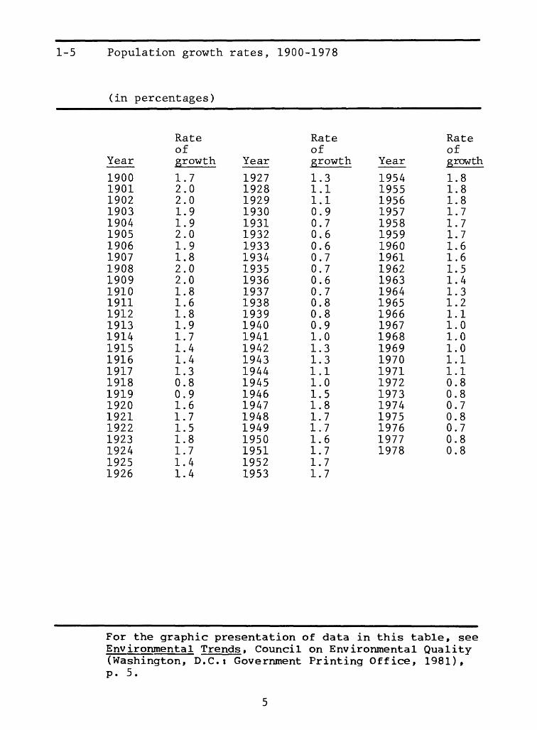
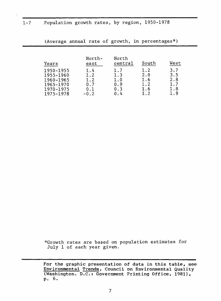
2025, 31-5 Population growth rates, 1900-1978, 5 1-6 Population, by region, 1950-1978, 6 1-7 Population growth rates, by region, 1950-1978, 1-8* Population density along major coasts, 1976 1-9 Increase in population density along major
coasts, 1940-1976, 8 1-10 Population in urban and rural areas, 1900-1950,
and in metropolitan and nonmetropolitan areas,1950-1978, 9
1-11* Metropolitan areas with population increases of20% or more, 1970-1977
1-12* Population migration, 1970-1978 1-13 Population growth rates in metropolitan and
nonmetropolitan counties, 1950-1977, 10 1-14* Population change in nonmetropolitan counties,
1970-1977 1-15* Urban regions, 2000
Chapter 2 Critical areas
Wetlands2-1* Natural wetlands, 19542-2 Total wetland acreage, presettlement to 1971,12 2-3 Wetland acreages, selected States, 1850-1964,13 2-4 Use of filled wetlands, Maine to Delaware, 1955-
1964, 15
*Map or diagram. Data not included in this book. For graphic presentation, see Environmental Trends, Council on Environmental Quality (Washington, D.C.:Government Printing Office, 1981).
111
2-5* State programs protecting wetlands and coastal areas, 1978
Wild areas2-6* National Wilderness Preservation System, 19782-7 Designated and proposed wilderness areas, 1964-
1979, 162-8* National Wild and Scenic Rivers, 1978 2-9 The National Wild and Scenic Rivers System,
1968-1978, 172-10* The National Park System, 1979 2-11 National Park Service units, 1872-1978, 18 2-12 National and State Park acreages, 1872-1978, 19 2-13* Representation of natural regions in the
National Park System, 19702-14 Visits to National and State Parks, 1954-1978, 20 2-15 Overnight stays in National Park Service-oper
ated campgrounds, 1960-1978, 21 2-16 The 10 most popular National Parks, 22
Historic places2-17 Properties on the National Register of Historic
Places, 1968-1978, 23 2-18 Properties on the National Register of Historic
Places, by type, 1978, 24 2-19 Properties removed from the National Register of
Historic Places, 1971-1978, 25
Risk zones2-20* Urban population and lands affected by stream
flooding, by Water Resources Region, 1967, 39 2-21* Hurricane risk along the Gulf and Atlantic
coasts2-22* Frequency of tornadoes, 1953-1962 2-23* Earthquake risk zones 2-24 Loss of life from selected natural disasters,
1900-1977, 26 2-25 Property damage from selected natural disasters,
1900-1977, 27
*Map or diagram. Data not included in this book. For graphic presentation, see Environmental Trends.
IV
Chapter 3 Human settlements
Settlement patterns3-1* Standard Metropolitan Statistical Areas, 1950 3-2* Standard Metropolitan Statistical Areas, 1978 3-3 Population in suburban areas and central cities,
1940-1978, 293-4 Population density, by location, 1940-1978, 30 3-5* Land use in Standard Metropolitan Statistical
Areas, by region, 1970
Housing units3-6 Composition of housing stock, by type of unit
and location, 1977, 31 3-7 Composition of housing stock, by type of unit,
1985, 59 4-14 Automobile emissions and standards, 1957-1985,
60 4-15 Noise levels of surface transportation vehicles,
1971. 61 4-16 Population exposed to noise at 23 major airports,
1972. 62
Chapter 5 Material use and solid waste
Material use5-1* Flow of materials, products, and solid wastes,
19775-2 U.S. material consumption, 1948-1978, 64 5-3 U.S. material consumption in relation to gross
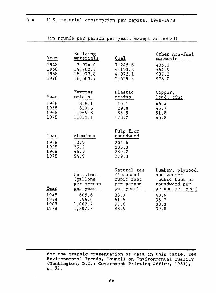
national product, 1948-1978, 65 5-4 U.S. material consumption per capita, 1948-
1978, 66
Solid waste5-5 Solid wastes disposed of by manufacturing
industries, 1974-1977, 67 5-6 Hazardous waste generated by selected industries,
1975, 68
*Map or diagram. Data not included in this book. For graphic presentation, see Environmental Trends.
VI
5-7* Industrial hazardous waste generation, by EPARegion, 1975
5-8 Consumer solid wastes disposed of and recycled,1960-1978, 69
5-9 Consumer solid wastes disposed of, by materials,1978, 70
5-10 Recycled consumer solid wastes, by material,1960-1978, 71
Chapter 6 Toxic substances
6-1* Selected toxic substances
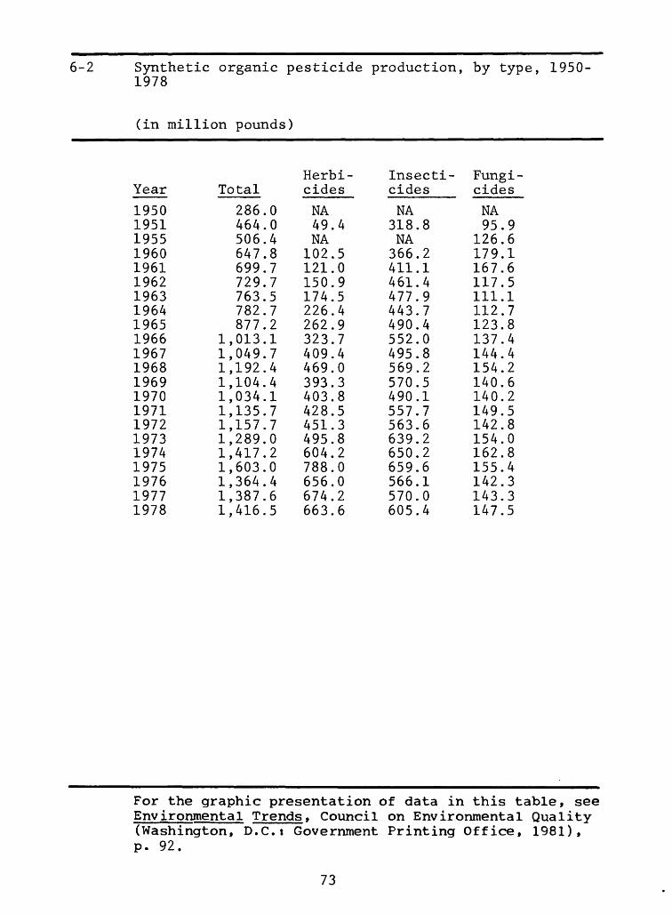
Pesticides6-2 Synthetic organic pesticide production, by
type, 1950-1978, 73 6-3 Insecticide production, by type of chemical,
1960-1978, 74 6-4 Selected herbicides used by farmers on crops,
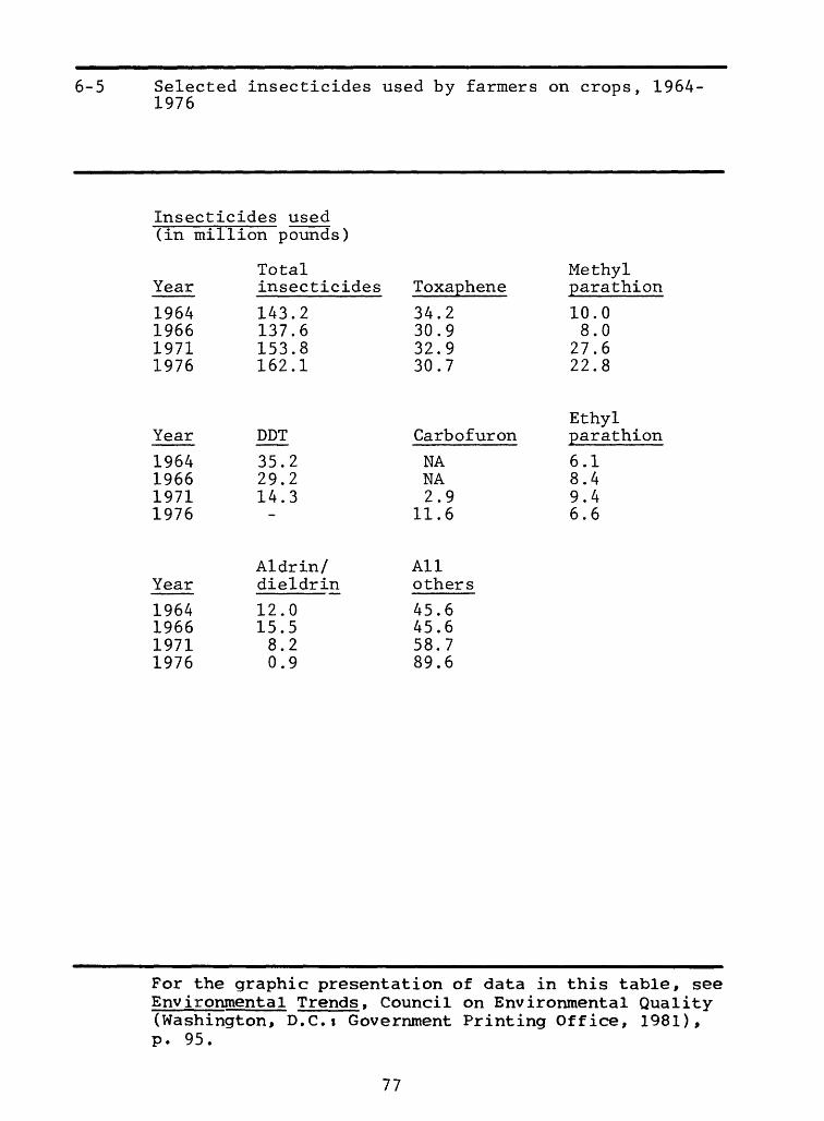
1964-1976, 75 6-5 Selected insecticides used by farmers on crops,
1964-1976, 77 6-6 Pesticide residues in river water and sediments
in Texas, Louisiana, and Oklahoma, 1968-1976,80 6-7 Pesticide residues in fish and birds, 1966-
1976, 81 6-8 Pesticide residues in human tissue, 1970-1976,
82
Industrial chemicals6-9 Production of selected industrial chemicals,
1950-1978, 836-10* Flow of asbestos in the environment 6-11 PCB residues in fish and birds, 1969-1976, 85 6-12 PCB residues in human tissue, 1972-1976, 86 6-13 Cancer deaths associated with vinyl chloride
and polyvinyl chloride, 1942-1973, 87 6-14 Cancer deaths associated with asbestos, 1959-
1977, 88
*Map or diagram. Data not included in this book. For graphic presentation, see Environmental Trends.
Vll
Metals6-15 Primary demand for selected metals, 1954-1978,
896-16* Flow of mercury in the environment 6-17 Cancer deaths associated with metals, 1940-1973,,
91
Radiation6-18 Radiation exposure, by source, 1970, 926-19 Radiation levels from nuclear fallout, as
measured by strontium-90 and cesium-137 inpasteurized milk, 1960-1978, 93
6-20 Radiation levels from nuclear power generation,as measured by krypton-85 in air, 1962-1976, 94
6-21* Radiation exposure of special population groups,1970s
6-22 Relative risk of cancer from radiation, 1946-1974, 95
Chapter 7 Cropland, forests, and rangeland
Cropland7-1* Cropland7-2 Uses of cropland, 1949-1978, 977-3* Prime farmland, 1975, 1197-4* Prime farmland lost to urbanization and water
projects, by farm production region, 1967-1975 7-5 Agricultural production, 1960-1978, 98 7-6 Agricultural inputs, 1950-1977, 99 7-7* Sheet and rill erosion from water on cropland,
by State, 1977 7-8* Wind erosion on cropland in the Great Plains
States, 1977
Forests7-9* Forests7-10* Ownership of forest land, 19777-11 Commercial forest land, by region and ecosystem,
1977, 102 7-12 Sawtimber growth and harvest, by type, 1952-
1976, 1047-13 Sawtimber growth and harvest, by region and ______ownership, 1952-1976, 105__________________
*Map or diagram. Data not included in this book. For graphic presentation, see Environmental Trends.
Vlll
7-14 Sawtimber growth and harvest in two regions, byownership, 1952-1976, 107
7-15 Roundwood harvest, by product, 1950-1976, 108 7-16 Forest conditions, 1950-1978, 110 7-17 Recreational use of the National Forests, 1965-
1977, 112 7-18 Recreational use of the National Forests, by
activity, 1977, 113
Rangeland 7-19* Rangeland7-20* Ownership of rangeland, 1977 7-21 Rangeland, by ecosystem, 1976, 114 7-22 Quality of rangeland, by ecosystem, 1976, 115 7-23 Productivity of rangeland, by ecosystem, 1976,
117
Chapter 8 Wildlife
8-1* Distribution of vertebrate species and major subspecies, by region, 1970s
Mammals8-2 Selected large mammal populations on Bureau of
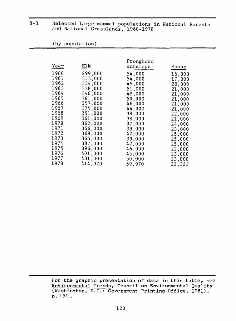
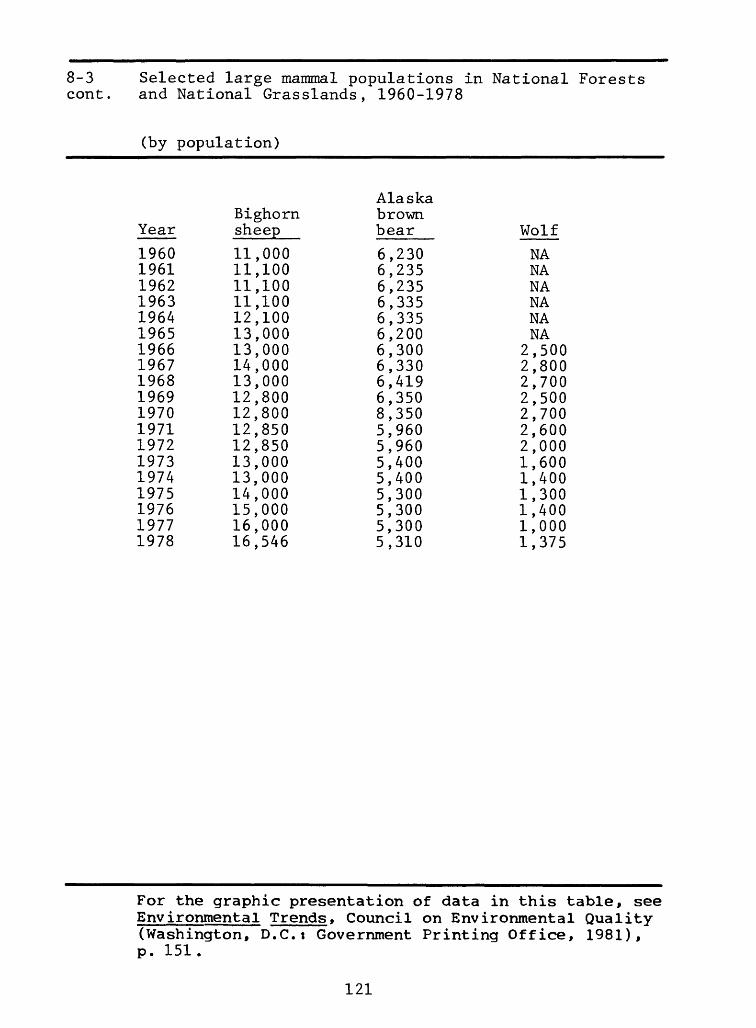
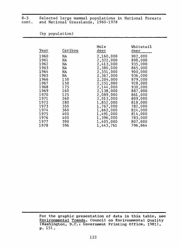
Land Management lands, 1961-1975, 119 8-3 Selected large mammal populations in National
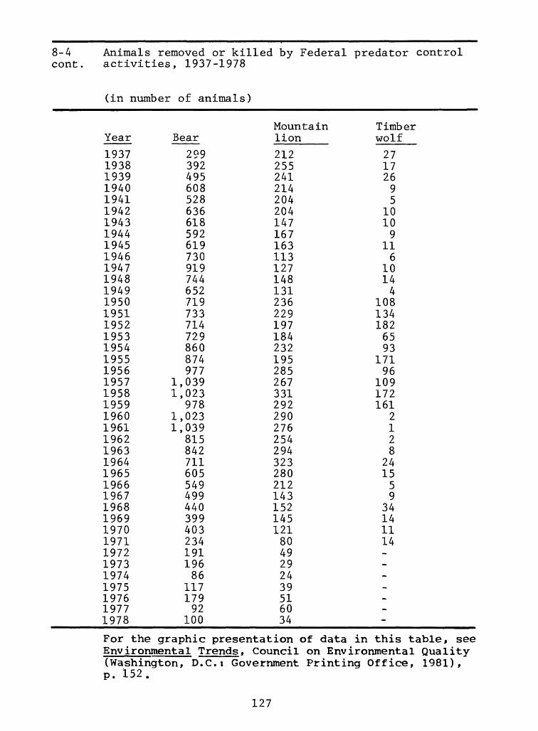
Forests and National Grasslands, 1960-1978, 120 8-4 Animals removed or killed by Federal predator
control activities, 1937-1978, 126
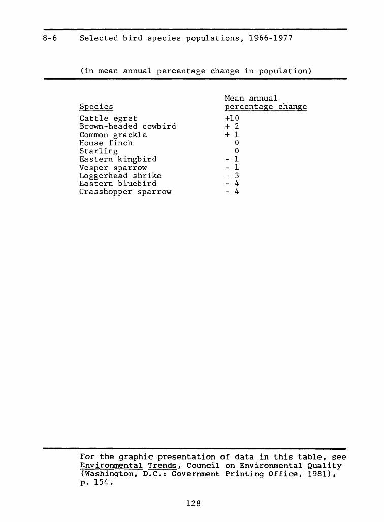
Birds8-5* Bird species observed, 1968-19778-6 Selected bird species populations, 1966-1977,
128 8-7 Most frequently observed breeding bird species,
1977, 129 8-8* Distribution of North American breeding and
wintering ducks, 1970s 8-9 Duck breeding populations in North America,
1955-1979, 1308-10 Duck harvest, by flyway, 1952-1978, 131 8-11 Brown pelican populations and toxic residues ______in eggs, 1969-1975, 132___________________
*Map or diagram. Data not included in this book. For graphic presentation, see Environmental Trends.
IX
Fish8-12* Distribution of fish species and major sub
species, by type of environment and region, 1970s
8-13 U.S. and foreign fish catch in U.S. waters, 1950-1979, 133
8-14 U.S. and foreign catch of selected fish species in U.S. waters, 1950-1979, 134
8-15* Estuarine habitat lost to dredging and filling, 1950-1969
8-16 Fish kills caused by pollution, 1961-1976, 137
Extinct, threatened, and endangered species8-17 Extinct vertebrate species and subspecies, 1960-
1979, 138 8-18 Threatened and endangered species in the United
States, December 1979, 139 8-19 Population of selected threatened and endangered
species, 1941-1979, 140 8-20* Condition of selected threatened and endangered
species
Chapter 9 Energy
Consumption and production9-1 Energy consumption, by fuel type, 1850-1978, 1429-2 Energy consumption, by fuel type, 1950-1978, 1429-3 Net trade in energy resources, 1950-1978, 1449-4 Energy production, by fuel type, 1850-1978,,1459-5 Energy production, by fuel type, 1950-1978, 1459-6* Energy flow in the U.S. economy, 19759-7 Energy consumption, by sector, 1950-1978, 1479-8 Energy consumption, by end use, 1950-1978, 1489-9 Residential heating, by fuel type, 1940-1975,
149 9-10* Residential heating, by fuel type and by county,
1970 9-11 Per capita energy consumption and gross domestic
product for four nations, 1961-1977, 150 9-12 Energy consumed by sector for nine nations, 1972,
154
*Map or diagram. Data not included in this book, graphic presentation, see Environmenta1 Trends.
For
x
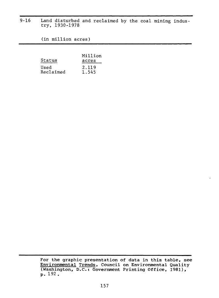
Fuel cycles9-13* Energy supply systems for fossil fuels9-14* Coal fields, 1970s9-15 Coal production, 1900-1978, 1559-16 Land disturbed and reclaimed by the coal mining
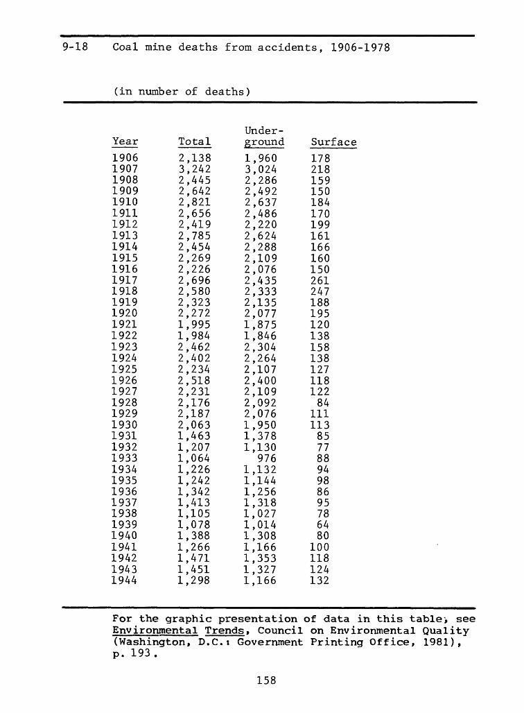
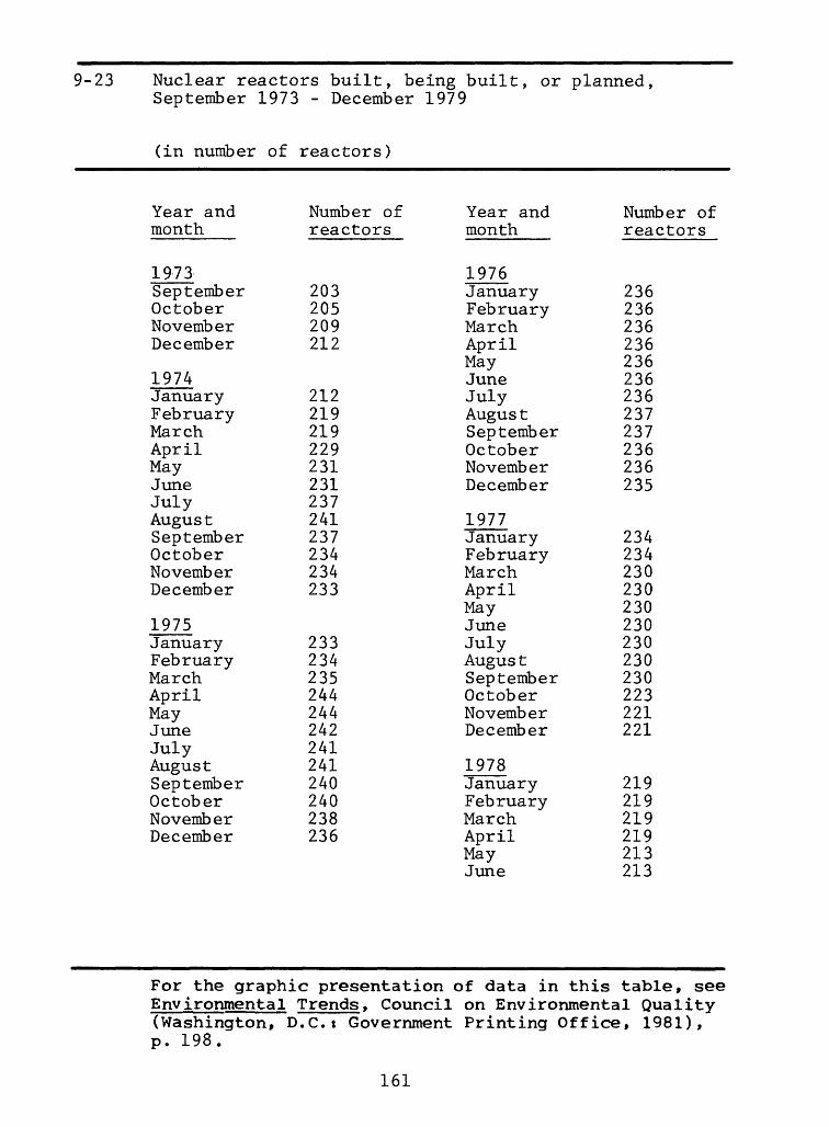
industry, 1930-1978, 1579-17* Streams affected by acid mine drainage, 1970s 9-18 Coal mine deaths from accidents, 1906-1978, 158 9-19* Natural gas and petroleum fields, 1970s 9-20 Natural gas and oil production, 1950-1978, 160 9-21* Liquified natural gas facilities, 1980 9_22* The nuclear fuel cycle 9-23 Nuclear reactors built, being built, or planned,
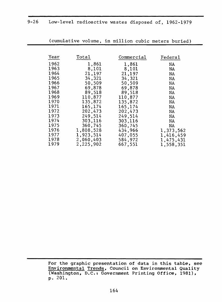
September 1973-December 1979, 161 9-24* Nuclear reactors, December 1979 9-25 Nuclear power generation, 1957-1979, 163 9-26 Low-level radioactive wastes disposed of, 1962-
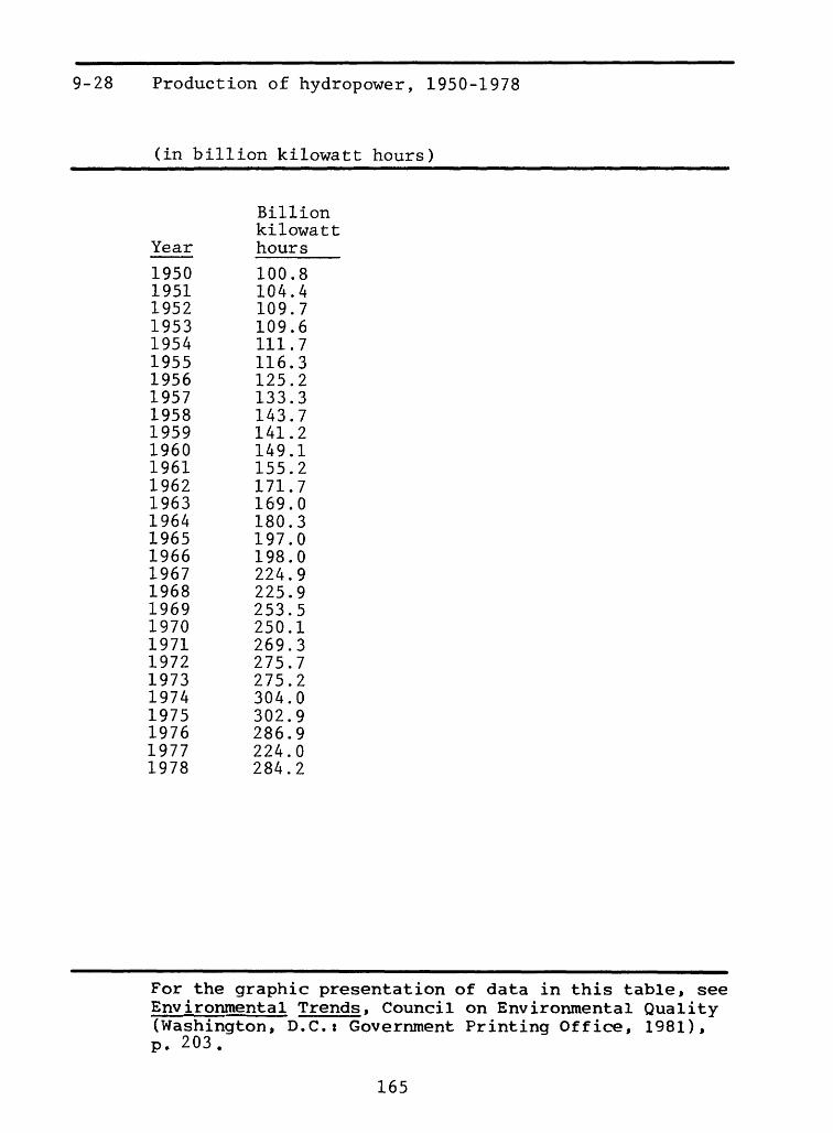
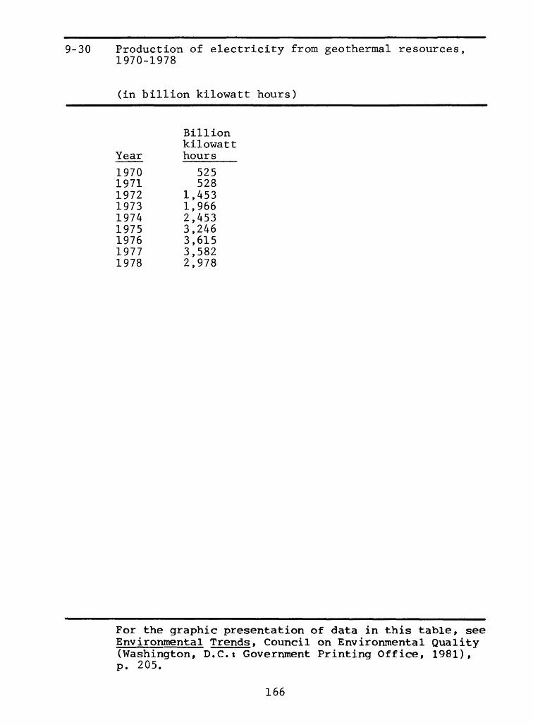
1979, 1649-27* Radioactive waste disposal sites, 1979 9-28 Production of hydropower, 1950-1978, 165 9-29* Geothertnal resources, 1970s 9-30 Production of electricity from geothermal
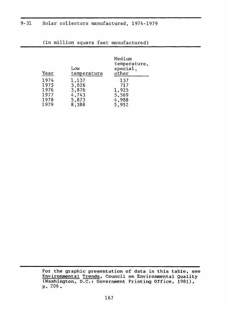
resources, 1970-1978, 166 9-31 Solar collectors manufactured, 1974-1979, 167
Chapter 10 Water resources
Abundance and distribution10-1* The hydrologic cycle10-2* Water resource regions, 197510-;3* Average annual precipitation, 1931-196010-4* Available ground water, 197510-5* Ground water withdrawals, 197510-6* Ground water overdraft, 197510-7* Average streamflow of large rivers, 1941-197010-8* Inadequate surface water supply for instream
use, 1975 10-9* Flooding problems, 1975
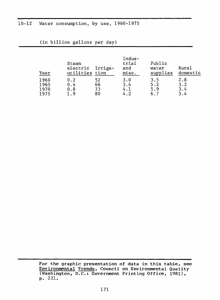
Use10-10 Water use, 1900-1975, 16910-11 Water withdrawal, by use, 1950-1975, 17010-12 Water consumption, by use, 1960-1975, 171
*Map or diagram. Data not included in this book. For graphic presentation, see Environmenta1 Trends.
XI
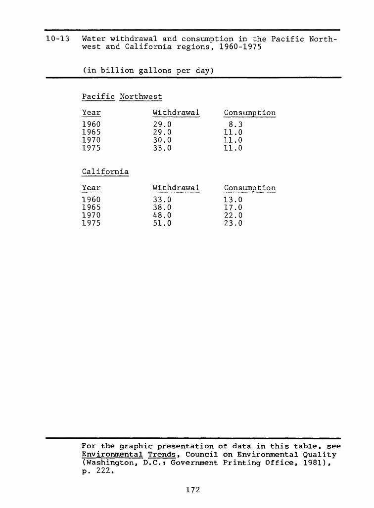
10-13 Water withdrawal and consumption in the PacificNorthwest and California regions, 1960-1975,172
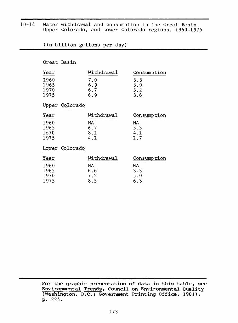
10-14 Water withdrawal and consumption in the GreatBasin, Upper Colorado, and Lower Coloradoregions, 1960-1975, 173
10-15 Water withdrawal and consumption in the Missouri,Arkansas-White-Red, Rio Grande, and Texas-Gulfregions, 1960-1975, 174
10-16 Water withdrawal and consumption in the Souris-Red-Rainy, Upper Mississippi, and Lower Missis sippi regions, 1960-1975, 175
10-17 Water withdrawal and consumption in the GreatLakes, Ohio, and Tennessee regions, 1960-1975,176
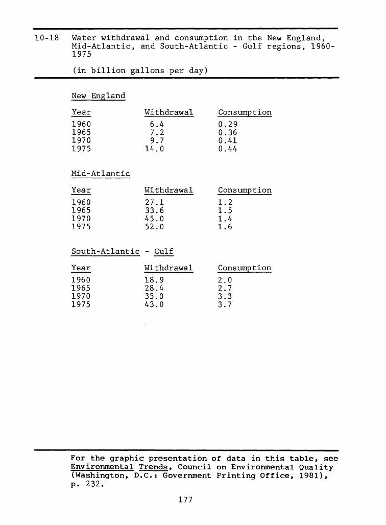
10-18 Water withdrawal and consumption in the NewEngland, Mid-Atlantic, and South Atlantic-Gulfregions, 1960-1975, 177
10-19 Water withdrawal and consumption in Alaska,Hawaii, and Caribbean regions, 1960-1975, 178
Chapter 11 Water quality
11-1* Sources and effects of water pollutants
Rivers and streams11-2 Fecal coliform bacteria, average annual viola
tion rates, 1975-1979, 18011-3* Fecal coliform bacteria in U.S. waters, 197811-4 Fecal coliform bacteria in major rivers, 1966-
1978, 18111-5 Dissolved oxygen, average annual violation
rates, 1975-1979, 18311-6* Dissolved oxygen in U.S. waters, 197811-7 Dissolved oxygen in major rivers, 1966-1978, 18411-8 Total phosphorus, average annual violation
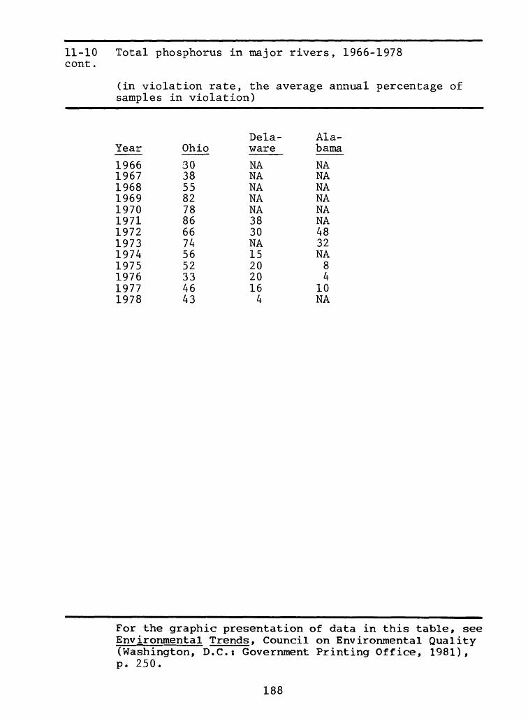
rates, 1975-1979, 18611-9* Total phosphorus in U.S. waters, 197811-10 Total phosphorus in major rivers, 1966-1976,18711-11* Heavy metals, 1975-197811-12 Phenols in the upper Ohio River basin, 1968-
1976, 18911-13 Discharges to water, by pollutant and by point
and nonpoint sources, 1977, 190
*Map or diagram. Data not included in this book, graphic presentation, see Environmental Trends.
For
XII
11-14* Point source discharges to water, by sector,1977
11-15 Population served by municipal wastewatersystems, by level of treatment, 1960-1978, 191
Lakes11-16 Eutrophication of U.S. lakes, 1975, 19211-17* Water quality problem areas of the Great Lakes,
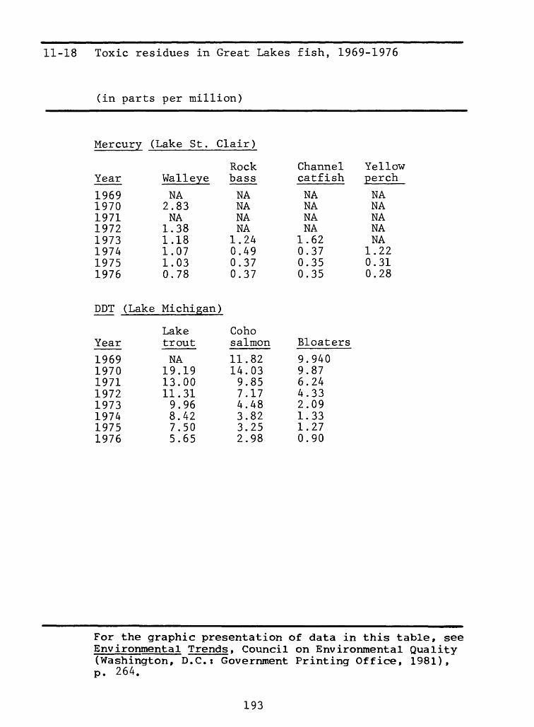
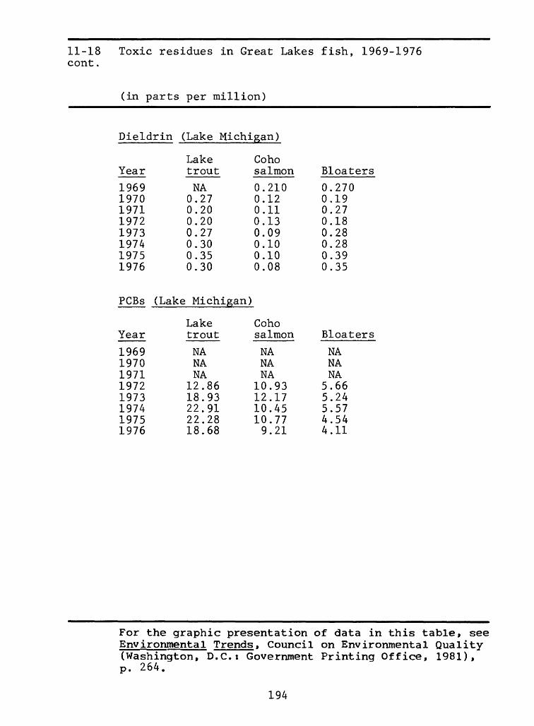
197811-18 Toxic residues in Great Lakes fish, 1969-1976,
193
Oceans11-19 Ocean dumping of U.S. wastes by barge, 1951-
1978, 19511-20 ( Oil spills in U.S. waters, 1971-1978, 196 11-21* Toxic residues in coastal mussels and oysters,
1976
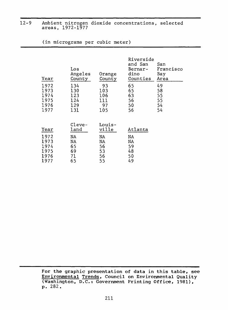
Chapter 12 Air quality
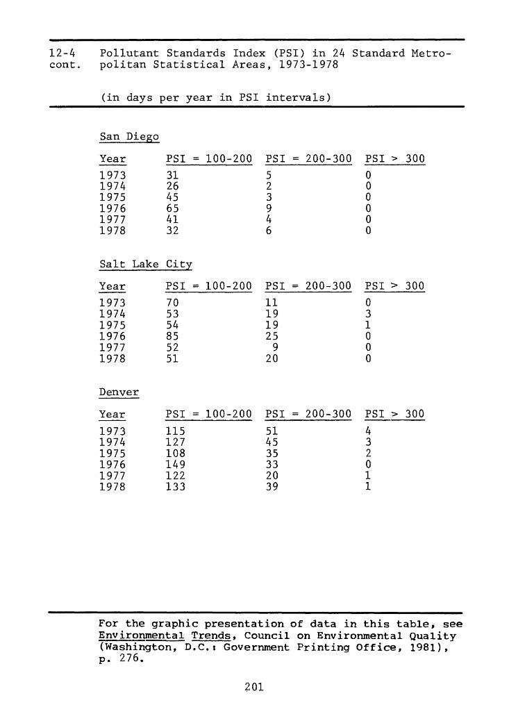
12-1* Criteria and noncriteria air pollutants 12-2* Pollutant Standards index values, pollutant
levels, and health effects
Ambient conditions12-3 Average Pollutant Standards Index for 23 Stan
combustion sources, by fuel type, 1970-1977,216 12-16 Sulfur oxide emissions, 1970-1977, 217 12-17 Sulfur oxide emissions from stationary fuel
combustion sources, by fuel type, 1970-1977,218 12-18 Total suspended particulate emissions, 1970-
1977, 219 12-19 Total suspended particulate emissions from
industrial sources, 1970-1977, 22012-20 Compliance status of major stationary air pollu
tion sources, 1975-1979, 22112-21 Compliance status of major stationary air pollu
tion sources, by industry, 1979, 222
Chapter 13 Biosphere
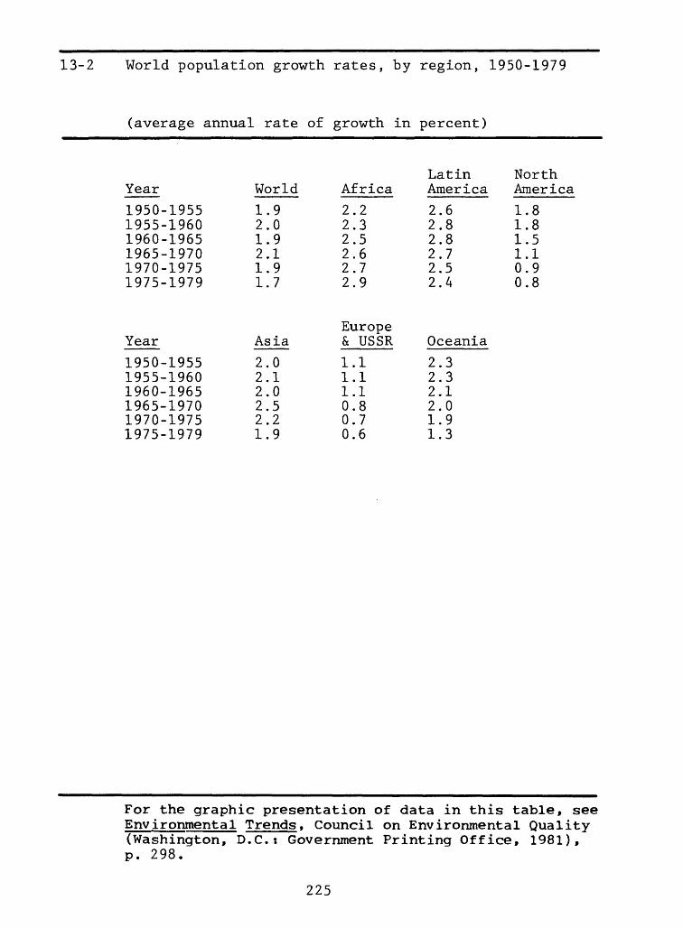
Population13-1 World population, by region, 1800-1979, 224 13-2 World population growth rates, by region, 1950-
1979, 22513-3* Population density, 1975 13-4 Population in urban and rural areas, by size,
1920-1975, 22613-5 Ten largest cities in the world, 1975, 227 13-6 Population by region, 1950-1979, with projections
to 2000, 228
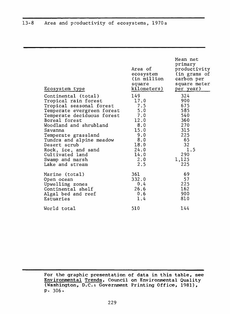
Land13-7* Major ecosystems of the world, 1970s13-8 Area and productivity of ecosystems, 1970s, 22913-9* Tropical moist forests, 1970s13-10 Tropical moist forests, by region and country,
1945-1978, 230 13-11* Lands vulnerable to desertification, 1970s
*Map or diagram. Data not included in this book. For graphic presentation, see Environmental Trends.
xiv
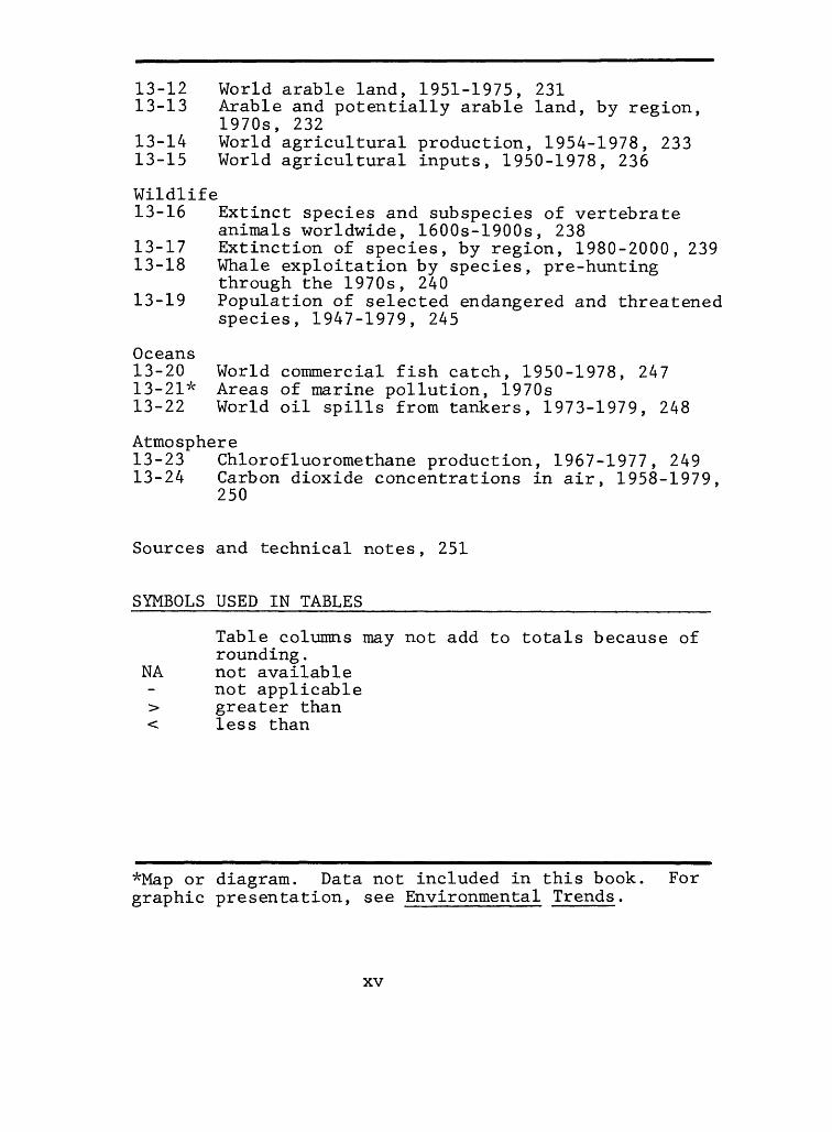
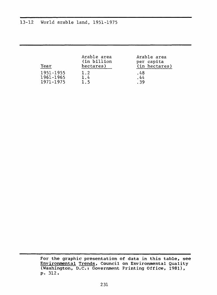
13-12 World arable land, 1951-1975, 23113-13 Arable and potentially arable land, by region,
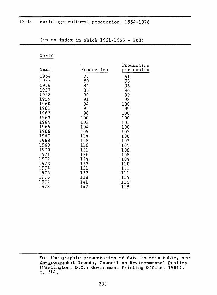
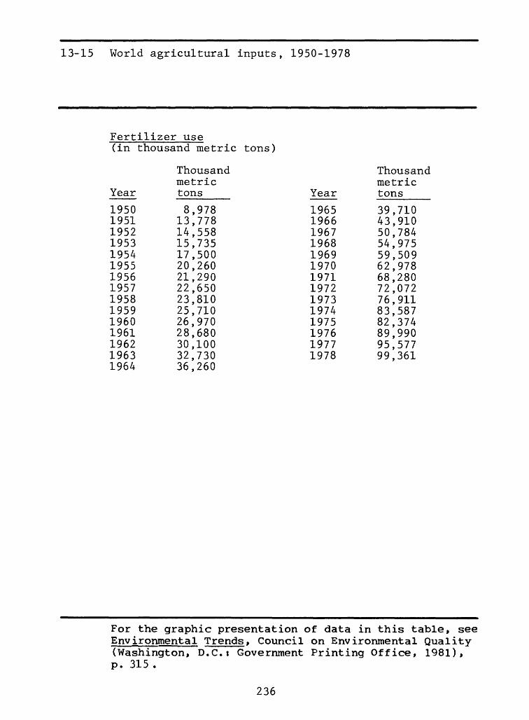
1970s, 23213-14 World agricultural production, 1954-1978, 233 13-15 World agricultural inputs, 1950-1978, 236
Wildlife13-16 Extinct species and subspecies of vertebrate
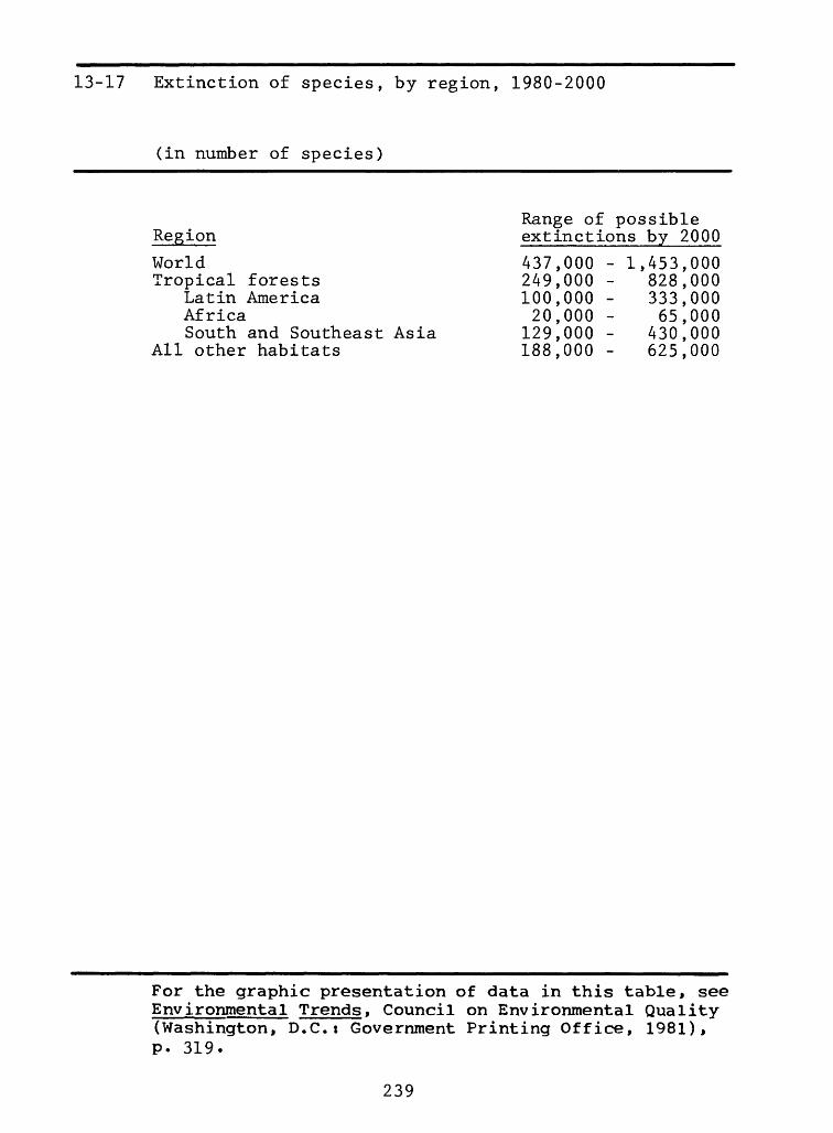
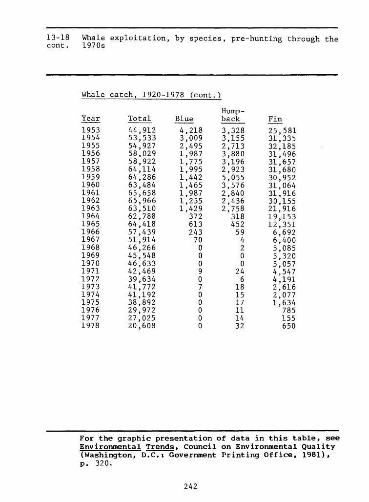
animals worldwide, 1600s-1900s, 23813-17 Extinction of species, by region, 1980-2000, 239 13-18 Whale exploitation by species, pre-hunting
through the 1970s, 240 13-19 Population of selected endangered and threatened
species, 1947-1979, 245
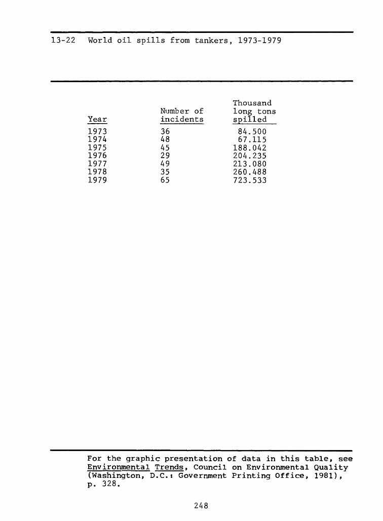
Oceans13-20 World commercial fish catch, 1950-1978, 24713-21* Areas of marine pollution, 1970s13-22 World oil spills from tankers, 1973-1979, 248
SYMBOLS USED IN TABLES____________________________
Table columns may not add to totals because ofrounding.
NA not availablenot applicable
> greater than < less than
*Map or diagram. Data not included in this book. For graphic presentation, see Environmental Trends.
xv
INTRODUCTION
In July, 1981, the Council on Environmental Quality published Environmental Trends. Composed of more than 250 charts, maps,diagrams,ind supportive text, Environmental Trends was conceived as a national briefing book that would provide policy makers, in and out of government, with readily accessible information to under stand better how natural and man-made environments were changing. Approximately 15,000 copies were distributed throughout the United States and abroad and sold through the Superintendent of Documents, U.S. Government Printing Office, Washington, D.C. 20402.
The project that culminated in the publication of Environmental Trends was begun in 1975 by the Council on Environmental Quality. The project was sponsored by the U.S. Geological Survey and the U.S. Fish and Wildlife Service, both of the Department of the Interior, the U.S. Environmental Protection Agency, and the Man and the Biosphere Program of the U.S. Department of State.
Supporting Data for Environmental Trends is a corn- pan ion~-cEcument to Environmental TrencTs. It has been compiled to provide analysts and researchers with the statistical data that were used to prepare the graphics in Environmental Trends. Supporting Data contains 185 tables, with sources and technical notes included at the back of the report.
The statistics in the tables were taken from various published and unpublished sources. Therefore, the number of significant figures for the same information may differ
The statistical tables were compiled by Daniel B. Tunstall, The Conservation Foundation. David W. Moody, U.S. Geological Survey, served as Contract Officer's Representative.
Chapter 1 PEOPLE AND THE LAND
1-4 Total population, 1900-1978, and projected to 2025
For the graphic presentation of data in this table, see Environmental Trends, Council on Environmental Quality (Washington, D.C.: Government Printing Office, 1981), p. 5.
1-4 Total population, 1900-1978, and projected to 2025 cont.
(in million people)
Series 1 Series 2 Series 3 projec- projec- projec-
For the graphic presentation of data in this table, see Environmental Trends, Council on Environmental Quality (Washington, D.C.j Government Printing Office, 1981), p. 5.
For the graphic presentation of data in this table, see Environmental Trends, Council on Environmental Quality (Washington, D.C.t Government Printing Office, 1981), p. 5.
For the graphic presentation of data in this table, see Env ironmental Trends, Council on Environmental Quality (Washington, D.C.t Government Printing Office, 1981), p. 6.
^Growth rates are based on population estimates for July 1 of each year given.
For the graphic presentation of data in this table, see Environmental Trends, Council on Environmental Quality (Washington. D.C.t Government Printing Office, 1981), p. 6.
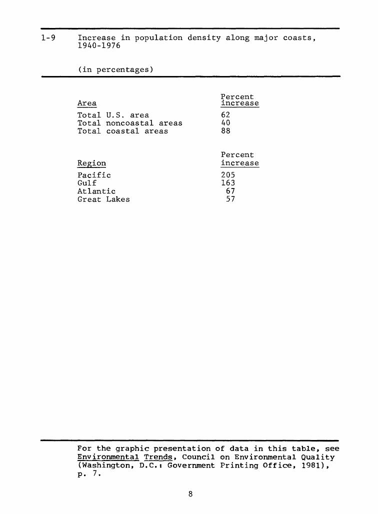
1-9 Increase in population density along major coasts, 1940-1976
(in percentages)
Percent Area increase
Total U.S. area 62Total noncoastal areas 40Total coastal areas 88
Percent Region increase
Pacific 205Gulf 163Atlantic 67Great Lakes 57
For the graphic presentation of data in this table, see Environmental Trends, Council on Environmental Quality (Washington, D.C.i Government Printing Office, 1981), p. 7.
8
1-10 Population in urban and rural areas, 1900-1950, and in metropolitan and nonmetropolitan areas, 1950-1978
(in million people)
Year1900 1910 1920 1930 1940 1950
Urban30.7 42.6 54.3 68.9 74.4 96.5
Rural45.4 49.3 51.4 53.8 57.2 54.2
Total76.0 92.0
105.7 122.8 131.7 150.7
Year
1950196019701978
SMSA, inside central city
53.759.962.959.7
SMSA, outside central city
40.959.674.283.3
Non-metro-politan
56.759.762.870.4
Total
151.3179.3199.8213.5
For the graphic presentation of data in this table, see Environmental Trends, Council on Environmental Quality (Washington, D.C.i Government Printing Office, 1981), p. 8.
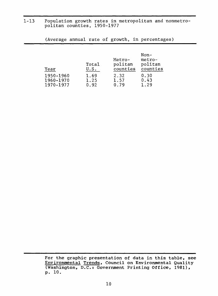
1-13 Population growth rates in metropolitan and nonmetro' politan counties, 1950-1977
For the graphic presentation of data in this table, see Environmental Trends, Council on Environmental Quality (Washington, D.C.i Government Printing Office, 1981), p. 10.
10
Chapter 2 CRITICAL AREAS
11
2-2 Total wetland acreage, presettlement to 1971
(in million acres)
Million Year acres
1700 1271922 911954 821971 70
For the graphic presentation of data in this table, see Environmental Trends, Council on Environmental Quality (Washington, D.C.t Government Printing Office, 1981), p. 18.
12
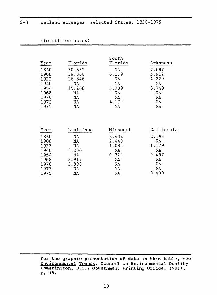
2-3 Wetland acreages, selected States, 1850-1975
(in million acres)
Year
185019061922194019541968197019731975
Florida
20.32519.80016.846NA
15.266NANANANA
SouthFlorida
NA6.179NANA
5.709NANA
4.172NA
Arkansas
7.6875.9124.220NA
3.749NANANANA
Year
185019061922194019541968197019731975
Louisiana
NANANA
4.206NA
3.911 3.890NANA
Missouri
3.4322.4401.085NA
0.322NA NA NA NA
California
2.193NA
1.179NA
0.457NANANA
0.400
For the graphic presentation of data in this table, see Environmental Trends, Council on Environmental Quality (Washington, D.C.i Government Printing Office, 1981), p. 19.
13
2-3 cont.
Wetland acreages, selected States, 1850-1975
(in thousand acres)
Year
18501930195419591964196819711974
Delaware
NANA
120.10 116.90 115.50
NANA
115.00
Mississippi
76.10 75.10NANANA
66.90NANA
Long Island, New York______
NANA
34.72 31.12 26.50 22.39 20.06NA
Year
Suffolk County, Long Island
NANA
20.59 19.21 17.00 12.93 10.83NA
Nassau County, Long Island
NA NA
14.1311.919.509.469.23NA
For the graphic presentation of data in this table, see Environmenta1 Trends, Council on Environmental Quality (Washington, D.C.t Government Printing Office, 1981), P. 19,
14
2-4 Use of filled wetlands, Maine to Delaware, 1955-1964
For the graphic presentation of data in this table, see Environmental Trends, Council on Environmental Quality (Washington, D.C.: Government Printing Office, 1981), p. 19.
15
2-7 Designated and proposed wilderness areas, 1964-1979
For the graphic presentation of data in this table, see Environmental Trends, Council on Environmental Quality (Washington, D.C.i Government Printing Office, 1981), P. 24.
16
2-9 The National Wild and Scenic Rivers System, 1968-1978
For the graphic presentation of data in this table, see Environmental Trends, Council on Environmental Quality (Washington, D.C.i Government Printing Office, 1981), p. 26.
For the graphic presentation of data in this table, see Environmental Trends, Council on Environmental Quality (Washington, D.C.t Government Printing Office, 1981), p. 30.
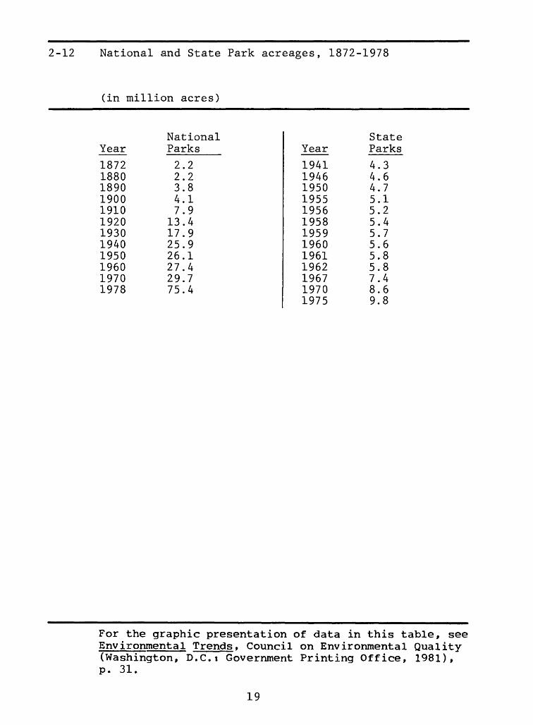
For the graphic presentation of data in this table, see Environmental Trends, Council on Environmental Quality (Washington, D.C.: Government Printing Office, 1981), p. 31.
19
2-14 Visits to National and State Parks, 1954-1978
For the graphic presentation of data in this table, see Environmental Trends, Council on Environmental Quality (Washington, D.C.i Government Printing Office, 1981), p. 33.
20
2-15 Overnight stays in National Park Service-operated campgrounds, 1960-1978
For the graphic presentation of data in this table, see E nv i ronmenta 1 Trends> Council on Environmental Quality (Washington, D.C.t Government Printing Office, 1981), P. 34.
21
2-16 The ten most popular National Parks, 1978
(in million visits)
Million Park visits
Great Smoky Mountains, Tennesseeand North Carolina 11.555
Hot Springs, Arkansas 5.421Grand Teton, Wyoming 4.160Acadia, Maine 3.130Rocky Mountain, Colorado 3.038Olympic, Washington 2.997Grand Canyon, Arizona 2.986Yosemite, California 2.669Yellowstone, Wyoming 2.623Mt. Rainier, Washington 2.094
For the graphic presentation of data in this table, see Environmental Trends, Council on Environmental Quality (Washington, D.C.: Government Printing Office, 1981), p. 35.
22
2-17 Properties on the National Register of Historic Places, 1968-1978
(in number of properties)
Year
NumberofProperties
6365
1,2002,2003,8005,9009,200
11,30013,50015,10018,300
For the graphic presentation of data in this table, see Environmental Trends, Council on Environmental Quality (Washington, D.C.: Government Printing Office, 1981), p. 36.
23
2-18 Properties on the National Register of Historic Places, by type, 1978
For the graphic presentation of data in this table, see Environmental Trends, Council on Environmental Quality (Washington, D.C.* Government Printing Office, 1981), p. 37.
24
2-19 Properties removed from the National Register of Historic Places, 1971-1978
For the graphic presentation of data in this table, see Environmental Trends, Council on Environmental Quality (Washington, D.C.t Government Printing Office, 1981), p. 37.
25
2-24 Loss of life from selected natural disasters, 1900-1977
(in average annual deaths per 10 million population)
For the graphic presentation of data in this table, see Environmental Trends, Council on Environmental Quality (Washington, D.C.t Government Printing Office, 1981), p. 42.
26
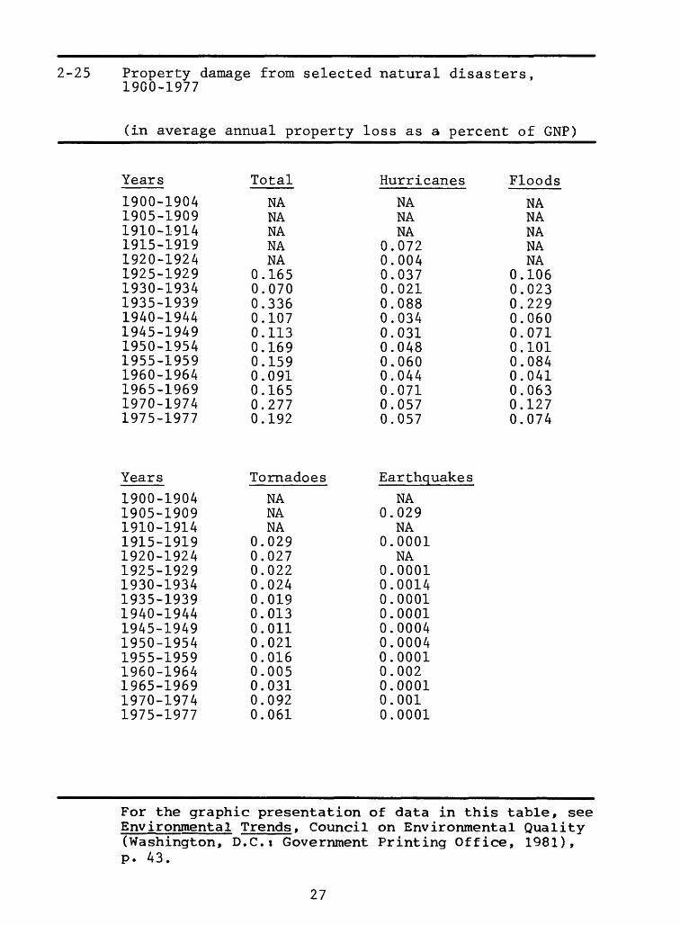
2-25 Property damage from selected natural disasters, 1900-1977
(in average annual property loss as a percent of GNP)
For the graphic presentation of data in this table, see Environmental Trends, Council on Environmental Quality (Washington, D.C.i Government Printing Office, 1981), p. 43.
27
Chapter 3 HUMAN SETTLEMENTS
28
3-3 Population in suburban areas and central cities, 1940-1978
For the graphic presentation of data in this table, see Environmental Trends, Council on Environmental Quality (Washington, D.C.t Government Printing Office, 1981), p. 48.
For the graphic presentation of data in this table, see Env ironmental Trends, Council on Environmental Quality (Washington, D.C.i Government Printing Office, 1981), p. 48.
30
3-6 Composition of housing stock, by type of unit and location, 1977
(in percentages)
Single Mobile Multi- Location family home family Total
Total U.S. 67.3 4.6 28.1 100 In SMSAs 61.5 3.0 35.5 100 Central cities
in SMSAs 49.5 1.0 49.6 100 Suburban areas
in SMSAs 71.6 4.6 23.8 100 Outside SMSAs
(nonmetropolitan) 79.4 8.0 12.6 100
For the graphic presentation of data in this table, see Environmental Trends, Council on Environmental Quality (Washington, D.C.t Government Printing Office, 1981), p. 50.
31
3-7 Composition of housing stock, by type of unit, 1940 1977
For the graphic presentation of data in this table, see Environmental Trends, Council on Environmental Quality (Washington, D.C.i Government Printing Office, 1981), p. 50.
For the graphic presentation of data in this table, see Environmenta1 Trends, Council on Environmental Quality (Washington, D.C.t Government Printing Office, 1981), p. 51.
33
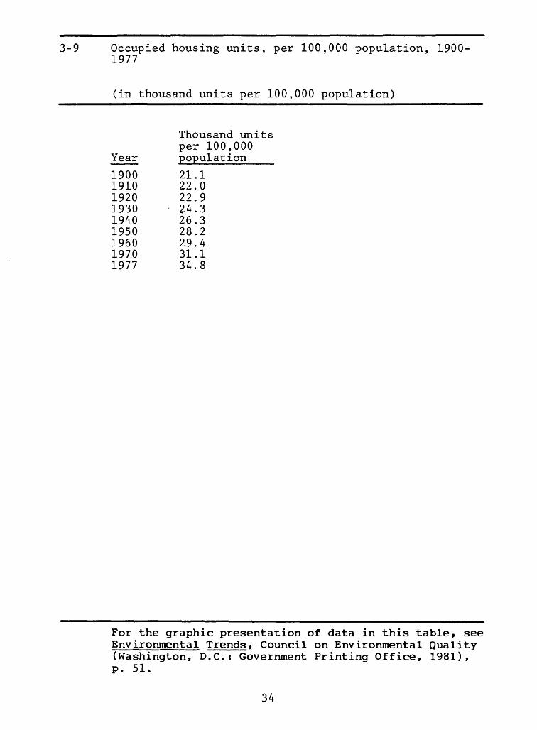
3-9 Occupied housing units, per 100,000 population, 1900 1977
For the graphic presentation of data in this table, see Environmental Trends, Council on Environmental Quality (Washington, D.C.: Government Printing Office, 1981), p. 51.
34
3-10 Characteristics of new single-family housing units, 1966-1978
For the graphic presentation of data in this table, see Environmental Trends, Council on Environmental Quality (Washington, D.C.t Government Printing Office, 1981), P. 52.
36
3-11 Characteristics of new multifamily housing units, 1971-1978
Size(in median square feet)
Year
19711972197319741975197619771978
Size
887892892922942894881863
Structure and facilities (in percent of units)
Year
19711972197319741975197619771978
Aircondi-tioning
NA NA NA 86 85 75 80 79
Electric heat___
NA NA NA 60 59 59 66 68
Two ormorebaths
NA NA NA 24 24192020
Four ormorefloors
16151616231488
For the graphic presentation of data in this table, see Environmental Trends, Council on Environmental Quality (Washington, D.C.j Government Printing Office, 1981), p. 53.
For the graphic presentation of data in this table, see Environmental Trends, Council on Environmental Quality (Washington, D.C.t Government Printing Office, 1981), p. 54.
38
3-13 Homes with selected major electric appliances, 1950 1977
(in percent of homes with appliances)
Year
1950 1955 1960 1965 1970 1974 1975 1976 1977
Air condi- tioning
0.8 5.6
15.1 24.2 40.6 51.6 52.8 54.4 55.3
Dish washers
2.0 4.0 7.1
13.5 26.5 36.6 38.3 39.6 40.9
Clothes dryers
1.4 9.2
19.6 26.4 44.6 56.5 57.7 58.6 59.3
Home freezers
7.2 16.8 23.4 27.2 31.2 41.7 43.5 44.4 44.8
Clothes washers
NA NA 55.4 57.4 62.1 68.4 69.9 72.5 73.3
For the graphic presentation of data in this table, see Environmental Trends, Council on Environmental Quality (Washington, D.C.t Government Printing Office, 1981), p. 55.
39
3-14 Overall opinion of living unit, by location, 1977
(in percentages)
Excel-Location
Total U.S.In SMSAsCentral cities
in SMSAsSuburban areas
in SMSAsOutside SMSAs
(nonmetropolitan)
lent
3434
28
39
32
.1
.7
.4
.8
.8
Good
47.46.
47.
46.
47.
07
4
1
6
Fair
15.15.
19.
11.
16.
52
5
6
2
Poor
2.2.
4.
2.
2.
99
1
0
8
For the graphic presentation of data in this table, see E nv i ronmenta1 Trends, Council on Environmental Quality (Washington, D.C.t Government Printing Office, 1981), p. 56.
40
3-15 Overall opinion of neighborhood, by location, 1977
(in percentages)
Excel- Location lent Good Fair Poor
Total U.S. 34.8 46.6 15.4 2.7 In SMSAs 33.7 46.2 16.5 3.1 Central cities
in SMSAs 26 47 22 5 Suburban areas
in SMSAs 40 46 12 2 Outside SMSAs
(nonmetropolitan) 37 48 13 2
For the graphic presentation of data in this table, see Env ironmental Trends, Council on Environmental Quality (Washington, D.C.s Government Printing Office, 1981), p. 56.
41
3-16 Inadequate neighborhood services, 1973-1977
(in percent of households)
Year
19731974197519761977
Year
19731974197519761977
Publictransportation
31.937.836.034.535.0
Fireprotection
NA4.94.34.8NA
Shopping
12.613.413.313.213.0
Schools
5.44.23.63.94.5
Hospitalsorhealthclinics Police
NA NA12.0 9.011.8 8.412.4 9.214.8 9.3
Outdoorrecreationfacilities
NANANANA23.0
For the graphic presentation of data in this table, see Env ironmental Trends , Council on Environmental Quality (Washington, D.C.i Government Printing Office, 1981), p. 57.
42
3-17 Neighborhood deficiencies, 1973-1977
(in percent reporting undesirable conditions)
Year
19731974197519761977
Year
19731974197519761977
Year
19731974197519761977
Noise
45.749.250.952.648.3
Odors
11.610.28.89.58.6
Inadequatestreetlights
19.921.025.024.424.8
Heavytraffic
28.931.430.230.429.1
Deterioratinghousing
8.610.19.5
10.010.2
Streetsneedrepair
14.119.417.117.518.3
Commercial/industrialuses
13.418.617.120.320.6
Abandonedhouses
5.86.86.87.17.0
Crime
13.217.118.417.816.9
For the graphic presentation of data in this table, see Environmental Trends, Council on Environmental Quality (Washington, D.C.t Government Printing Office, 1981), P. 58.
43
3-17 Neighborhood deficiencies, 1973-1977 cont.
(in percent reporting undesirable conditions)
Want to move because of one or more
Impassable of above Year Litter roads____ conditions
For the graphic presentation of data in this table, see Environmental Trends, Council on Environmental Quality (Washington, D.C.t Government Printing Office, 1981), p. 58.
For the graphic presentation of data in this table, see Environmental Trends, Council on Environmental Quality (Washington, D.C.i Government Printing Office, 1981), p. 62.
46
4-1 Major transportation networks, 1925-1978 cont .
For the graphic presentation of data in this table, see Environmental Trends, Council on Environmental Quality (Washington, D.C.j Government Printing Office, 1981), p. 62.
For the graphic presentation of data in this table, see Environmental Trends, Council on Environmental Quality (Washington, D.C.t Government Printing Office, 1981), p. 62.
For the graphic presentation of data in this table, see Environmental Trends, Council on Environmental Quality (Washington, D.C.i Government Printing Office, 1981), p. 62.
For the graphic presentation of data in this table, see Environmental Trends, Council on Environmental Quality (Washington, D.C.t Government Printing Office, 1981), p. 63.
50
4-4 Local passenger travel, 1950-1975
(in passenger-miles per capita)
School Transit Rail CommuterYear Auto bus bus transit rail
For the graphic presentation of data in this table, see Environmental Trends, Council on Environmental Quality (Washington, D.C.i Government Printing Office, 1981), p. 63.
51
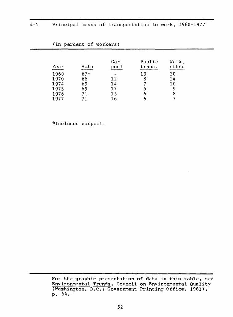
4-5 Principal means of transportation to work, 1960-1977
For the graphic presentation of data in this table, see Environmental Trends, Council on Environmental Quality (Washington, D.C.t Government Printing Office, 1981), p. 64.
52
4-6 Principal means of transportation to work, by location, 1977
(in percent of workers)
Location
Total U.S.In SMSAsCentral cities
in SMSAsSuburban areas
in SMSAsOutside SMSAs
(nonmetropolitan)
Auto
7171
65
76
69
Car-pool
1615
14
16
19
Publictrans .
68
13
3
1
Walk,other
76
7
5
11
For the graphic presentation of data in this table, see Environmental Trends, Council on Environmental Quality (Washington, D.C.i Government Printing Office, 1981), p. 64.
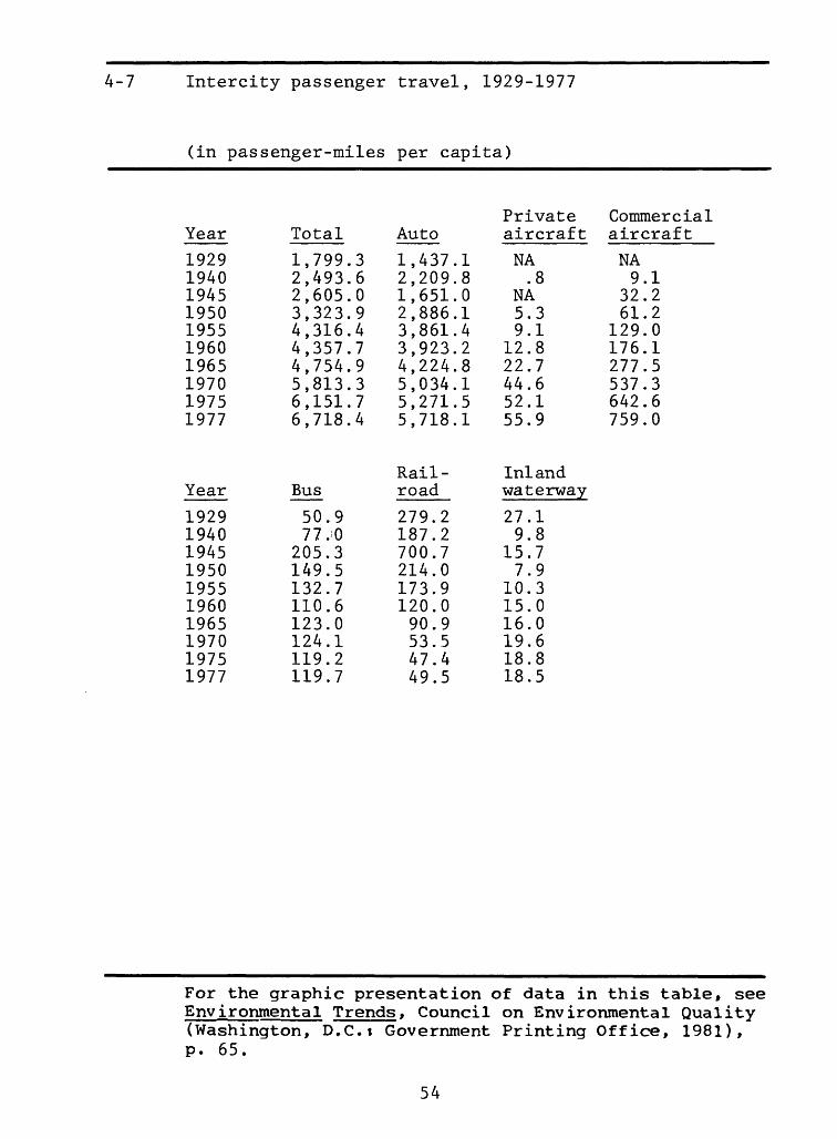
For the graphic presentation of data in this table, see Environmental Trends, Council on Environmental Quality (Washington, D.C.i Government Printing Office, 1981), p. 65.
For the graphic presentation of data in this table, see Environmental Trends, Council on Environmental Quality (Washington, D.C.t Government Printing Office, 1981), p. 65.
55
4-10 Energy consumption, by mode of transportation, 1965 1977
(in quads*)
Year
1965197019751977
Total, all modes
11,863.915,797.417,731.019,251.0
Total highway
8,942.011,629.413,750.015,122.9
Auto
6,273.48,203.09,497.6
10,028.2
Year
1965197019751977
Bus
120.0126.6119.2132.3
Truck
2,540.03,282.94,077.34,906.0
Rail
575.3543.6576.6609.8
Year
1965197019751977
Air
740.01,652.11,529.81,616.9
Water
565.5753.3851.3
1,102.8
Pipeline
517.0744.6595.2561.6
*0ne quad is the equivalent of 15.8 billion barrels of oil.
For the graphic presentation of data in this table, see Environmental Trends, Council on Environmental Quality (Washington, D.C.» Government Printing Office, 1981), p. 67.
56
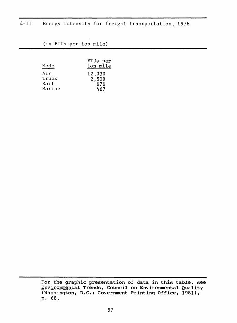
4-11 Energy intensity for freight transportation, 1976
(in BTUs per ton-mile)
BTUs per Mode ton-mile
Air 12,030Truck 2,500Rail 676Marine 467
For the graphic presentation of data in this table, see Environmental Trends, Council on Environmental Quality (Washington, D.C.t Government Printing Office, 1981), p. 68.
57
4-12 Energy intensity for local and intercity passenger travel, 1976
(in BTUs per passenger-mile)
Local passenger travel
BTUs per Mode pas senger-mile
Auto 4,310Transit rail 3,030Bus 2,960
Intercity passenger travel
BTUs per Mode passenger-mile
Air 6,760Auto 4,310Rail 3,230Bus 1,010
For the graphic presentation of data in this table, see E nv i ronmenta1 Trends, Council on Environmental Quality (Washington, D.C.i Government Printing Office, 1981), p. 68.
58
4-13 Automobile fuel economy and standards, 1940-1985
For the graphic presentation of data in this table, see Environmental Trends, Council on Environmental Quality(Washington, D.C.t Government Printing Office, 1981), p. 69.
59
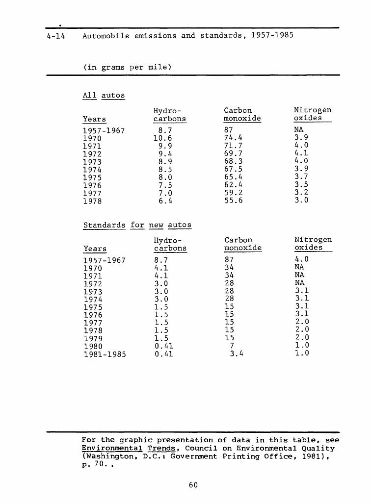
4-14 Automobile emissions and standards, 1957-1985
For the graphic presentation of data in this table, see Environmental Trends, Council on Environmental Quality (Washington, D.C.i Government Printing Office, 1981), p. 70. .
60
4-15 Noise levels of surface transportation vehicles, 1971
(in decibels at 50 feet)
Highway
Mode
Heavy trucks Motorcycles Garbage trucks Highway buses Automobiles (sport) City buses Light trucks Automobiles (standard)
Decibels at 50 feet
8482828275737269
Rail
Mode
TrainsRapid transit
Decibels at 50 feet
9486
Recreational vehicles
Mode
Off-road motorcyclesSnowmobilesMotor boats
Decibels at 50 feet
858580
For the graphic presentation of data in this table, see Environmental Trends, Council on Environmental Quality (Washington, D.C.t Government Printing Office, 1981), p. 71.
61
4-16 Population exposed to noise at 23 major airports, 1972
(in thousand people exposed)
Airport
Atlanta Boston Buffalo Chicago:MidwayO'Hare
Cleveland Denver Los Angeles Miami Minneapolis-
St. Paul New York:
KennedyLa Guardia
New Orleans NewarkPhiladelphia Phoenix Portland San Diego San Francisco Seattle St. Louis Washington, D.C
DullesNational
Noise level in excess of NEF 30*
99.8431.3113.8
38.5771.7128.7180.3292.4260.0
96.7
507.31057.0
32.5431.976.920.51.2
77.3124.1123.2100.0
3.5 24.4
Noise level in excess of NEF 40*
27.0329.7
1.866.611.228.351.129.7
8.8
111.517.18.9
27.50.36.20.3
24.011.417.38.5
0.0 2.0
*NEF, noise exposure forecast, is the total aircraft- generated noise measured at locations near an airport during a typical 24 hours.
For the graphic presentation of data in this table, see Environmental Trends, Council on Environmental Quality (Washington, D.C.t Government Printing Office, 1981), P. 72.
62
Chapter 5 MATERIAL USE AND SOLID WASTE
63
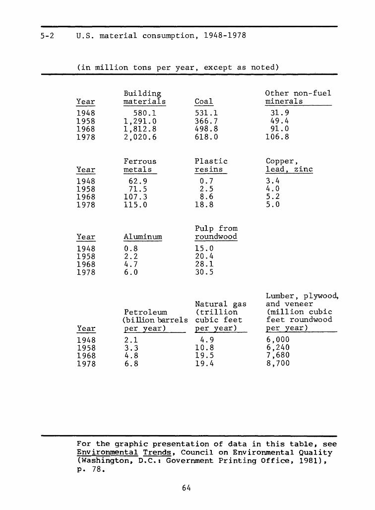
5-2 U.S. material consumption, 1948-1978
(in million tons per year, except as noted)
Year
1948 1958 1968 1978
Year
1948 1958 1968 1978
Year
1948 1958 1968 1978
Building materials
580.1 1,291.0 1,812.8 2,020.6
Ferrous metals
62.9 71.5
107.3 115.0
Aluminum
0.8 2.2 4.7 6.0
Coal
531.1 366.7 498.8 618.0
Plastic resins
0.7 2.5 8.6
18.8
Pulp from roundwood
15.0 20.4 28.1 30.5
Other non-fuel minerals
31.9 49.4 91.0
106.8
Copper , lead, zinc
3.4 4.0 5.2 5.0
Year
1948195819681978
Natural gasPetroleum (trillion (billion barrels cubic feet per year)___ per year)
2.1 3.3 4.8 6.8
4.910.819.519.4
Lumber, plywood, and veneer (million cubic feet roundwood per year)_____
6,0006,2407,6808,700
For the graphic presentation of data in this table, see Environmental Trends, Council on Environmental Quality (Washington, D.C.t Government Printing Office, 1981), p. 78.
64
5-3 U.S. material consumption in relation to gross national product, 1948-1978
(in tons consumed per million dollars GNP, except as noted)
Year
1948 1958 1968 1978
Year
1948195819681978
Year
1948195819681978
Building materials
1,189.4 1,851.4 1,723.5 1,458.6
Ferrous metals
128.9102.5102.083.0
Aluminum
1.63.14.44.3
Coal
1,089.0 525.9 474.2 446.1
Plastic resins
1.53.68.2
13.6
Pulp from roundwood
30.829.326.722.0
Other non-fuel minerals
65.4 70.8 86.5 77.1
Copper , lead, zinc
7.05.74.93.6
Year
1948195819681978
Petroleum (barrels consumed per
Natural gas (thousand cubic feet consumed per
Lumber, plywood and veneer (thousand cubic feet of round- wood consumedper
million $ GNP) million $ GNP) million $ GNP)
4,3354,7544,5534,924
10,14015,43018,50014,010
12.38.957.36.3
For the graphic presentation of data in this table, see Environmental Trends, Council on Environmental Quality (Washington, D.C.t Government Printing Office, 1981), p. 80.
65
5-4 U.S. material consumption per capita, 1948-1978
(in pounds per person per year, except as noted)
Year
1948195819681978
Building materials
7,914.014,762.718,073.818,503.7
Coal
7,245.64,193.34,973.15,659.3
Other non-fuel minerals_____
435.2564.9907.3978.0
Year
1948195819681978
Ferrous metals
858.1817.6
1,069.81,053.1
Plastic resins
10.129.085.9
178.2
Copper, lead, zinc
46.445.751.845.8
Year
1948195819681978
Aluminum
10.925.246.954.9
Pulp from roundwood
204.6233.3280.2279.3
Year
1948195819681978
Petroleum (gallons per person per year)
605.6796.0
1,002.71,307.7
Natural gas (thousand cubic feet per person per year)33.761.597.088.9
Lumber, plywood, and veneer (cubic feet of roundwood per person per year)40.935.738.339.8
For the graphic presentation of data in this table, see Environmental Trends, Council on Environmental Quality (Washington, D.C.t Government Printing Office, 1981), p. 82.
66
5-5 Solid wastes disposed of by manufacturing industries, 1974-1977
(in million short tons)
Year
1974 1975 1976 1977
Year
1974 1975 1976 1977
Year
1974 1975 1976 1977
Year
1974 1975 1976 1977
Total manufacturing
133.3 139.1 156.8 160.0
Food processing
11.6 12.6 15.0 13.1
Lumber
6.9 8.1 9.3 6.3
Petroleum and coal2.4 2.0 2.6 2.9
Chemicals
38.2 38.7 50.3 55.7
Stone, clay, glass
9.3 11.3 11.1 12.6
Trans portation
4.2 3.8 4.3 4.7
Fabricated metal
2.1 1.9 2.1 2.0
Primary metals
40.8 42.7 42.4 41.7
Paper
8.8 9.1
10.1 10.6
Machinery
2.7 2.7 3.1 3.6
For the graphic presentation of data in this table, see Environmental Trends, Council on Environmental Quality (Washington, D.C.t Government Printing Office, 1981), p. 84.
67
5-6 Hazardous waste generated by selected industries, 1975
(in million metric tons per year, wet weight)
Industry
Primary metals, smelting,and refining
Organic chemicals,pesticides, and explosives
Electroplating Inorganic chemicals Textile dying and finishing Petroleum refining Rubber and plastics
Million metric tons per year
8.27
862840777679
For the graphic presentation of data in this table, see Environmental Trends, Council on Environmental Quality (Washington, D.C.t Government Printing Office, 1981), P. 85.
68
5-8 Consumer solid wastes disposed of and recycled, 1960 1978
For the graphic presentation of data in this table, see Environmental Trends, Council on Environmental Quality (Washington, D.C.t Government Printing Office, 1981), p. 86.
69
5-9 Consumer solid wastes disposed of, by materials, 1978
(in million tons)
Type of waste Million tons
Total 150Paper 52Yard 27Food 23Glass 15Metals 13Miscellaneous 20
For the graphic presentation of data in this table, see Environmental Trends, Council on Environmental Quality (Washington, D.C.: Government Printing Office, 1981), p. 86.
70
5-10 Recycled consumer solid wastes, by material, 1960-1978
(in percent of gross discards recycled)
Year
19601965197019711972197319741975197619771978
Year
19601965197019711972197319741975197619771978
Paper andpaperboard
18.815.816.015.916.016.516.315.516.119.820.1
Glass
1.41.21.31.82.12.32.52.72.73.43.3
Aluminum
NANA1.32.43.23.45.08.79.27.1
13.3
Rubber
5.712.58.28.97.96.86.16.93.93.43.3
Ferrousmetals
0.51.01.21.31.42.43.44.44.52.52.5
For the graphic presentation of data in this table, see Environmental Trends, Council on Environmental Quality (Washington, D.C.: Government Printing Office, 1981), p. 87.
71
Chapter 6 TOXIC SUBSTANCES
72
6-2 Synthetic organic pesticide production, by type, 1950 1978
For the graphic presentation of data in this table, see Environmental Trends, Council on Environmental Quality (Washington, D.C.s Government Printing Office, 1981), p. 92.
73
6-3 Insecticide production, by type of chemical, 1960-1978
(in million pounds)
Organo- Organo-Total chlorine phosphorous
Year insecticides insecticides insecticides
1960 366 NA NA1961 411 NA NA1962 461 NA NA1963 478 285 741964 444 229 811965 490 260 951966 552 272 1201967 496 224 NA1968 569 255 NA1969 571 NA NA1970 490 148 1321971 558 165 1381972 564 208 1611973 639 220 1731974 650 207 1871975 660 172 2131976 566 150 1901977 570 NA 2041978 605 NA 208
For the graphic presentation of data in this table, see Environmental Trends, Council on Environmental Quality (Washington, D.C.t Government Printing Office, 1981), p. 93.
74
6-4 Selected herbicides used by farmers on crops, 1964-1976
Herbicides used(in million pounds)
Year
1964 1966 1971 1976
Year
1964 1966 1971 1976
Acres
Total herbicides
76.3 112.4 224.0 394.0
2,4-D
29.7 39.5 33.3 38.4
treated(in million acres)
Year
1964 1966 1971 1976
Year
1964 1966 1971 1976
Total herbicides
NA 98.7
157.8 196.6
2,4-D
56.3 56.9 54.8 58.6
Atrazine
10.823.557.290.3
Trifluralin
NA5.2
11.4 28.3
Atrazine
7.915.039.861.8
Trifluralin
NA6.9
16.6 33.7
Alachlor
NANA
14.8 88.5
All Others
35.844.2
107.3148.7
Alachlor
NANA
11.6 53.5
For the graphic presentation of data in this table, see Environmental Trends, Council on Environmental Quality (Washington, D.C.t Government Printing Office, 1981), p. 94.
75
6-4 cont.
Selected herbicides used by farmers on crops, 1964-1976
Pounds used per acre (in pounds per acre)
Year
1964196619711976
Average, all herbicides
NA 1.1 1.4 2.0
Atrazine
1.4 1.61.41.5
Alachlor
NANA 1.3 1.7
Year
1964196619711976
2,4-D
0.5 0.7 0.6 0.7
TrifluralinNA
0.7 0.7 0.8
For the graphic presentation of data in this table, see Environmental Trends, Council on Environmental Quality (Washington, D.C.t Government Printing Office, 1981), p. 94.
76
6-5 Selected insecticides used by farmers on crops, 1964 1976
Insecticides used (in million pounds)
YearTotal insecticides
143.2137.6153.8162.1
Toxaphene
34.230.932.930.7
Methyl parathion
10.08.0
27.622.8
Year DPT
35.229.214.3
Carbofuron
NA NA 2.9
11.6
Ethyl parathion
6.1 8.4 9.4 6.6
YearAldrin/ dieldrin
12.015.58.20.9
All others
45.645.658.789.6
For the graphic presentation of data in this table, see Environmental Trends, Council on Environmental Quality (Washington, D.C.i Government Printing Office, 1981), p. 95.
77
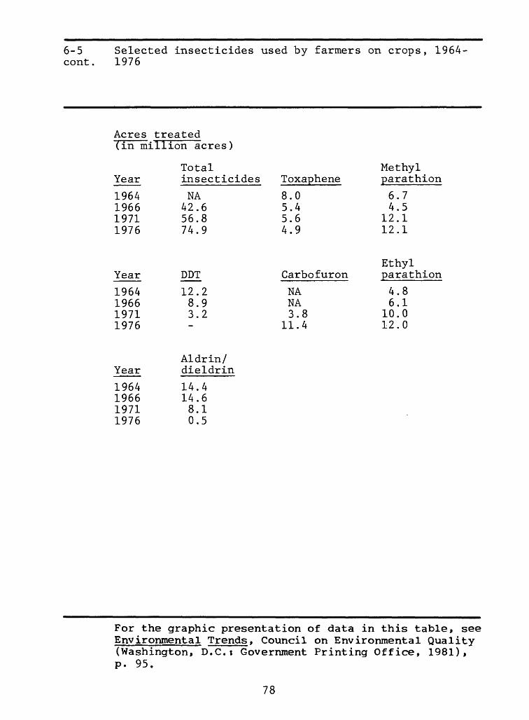
6-5 Selected insecticides used by farmers on crops, 1964 cont. 1976
Acres treated(in million acres)
YearTotal insecticides
NA 42.6 56.8 74.9
Toxaphene
8.0 5.4 5.6 4.9
Methyl parathion
6.74.5
12.112.1
Year
1964196619711976
DPT
12.2 8.9 3.2
Carbofuron
NA NA 3.8
11.4
Ethyl parathion
4.86.1
10.012.0
Year
1964196619711976
Aldrin/ dieldrin
14.414.68.10.5
For the graphic presentation of data in this table, see Environmental Trends, Council on Environmental Quality (Washington, D.C.t Government Printing Office, 1981), p. 95.
78
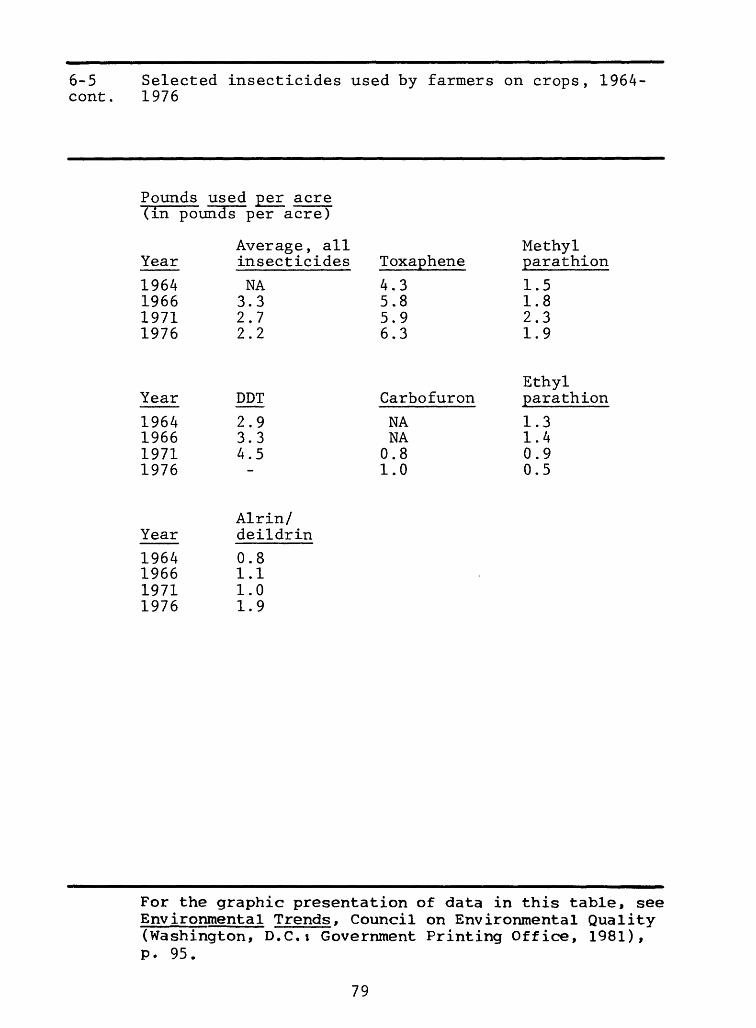
6-5 Selected insecticides used by farmers on crops, 1964 cont. 1976
Pounds used per acre (in pounds per acre)
YearAverage, all insecticides
NA 3.3 2.7 2.2
Toxaphene
4.35.85.9 6.3
Methyl parathion
1.5 1.8 2.3 1.9
Year
1964196619711976
DPT
2.9 3.3 4.5
Carbofuron
NANA 0.8 1.0
Ethyl parathion
1.31.4 0.9 0.5
YearAlrin/ deildrin
0.8 1.1 1.0 1.9
For the graphic presentation of data in this table, see Environmental Trends, Council on Environmental Quality (Washington, D.C.j Government Printing Office, 1981), P. 95.
79
6-6 Pesticide residues in river water and sediments in Texas, Louisiana, and Oklahoma, 1968-1976
(in percent of samples with residues)
DDT
Year
1968 1969 1970 1971 1972 1973 1974 1975 1976
Water
36 38 37 27 21 17 6 5 4
Sedi ments
NA NA 89
100 77 36 40 33 27
Aldrin
Year
1968 1969 1970 1971 1972 1973 1974 1975 1976
Water
1 NA 2
NA NA 1 3 0 0
Sedi ments
NA NA 81
100 66 1 2 2 2
Dieldrin
Year
196819691970197119721973197419751976
Chlordane
Water
143731474428292221
Sediments
NANA87
1007531434936
Year
196819691970197119621973197419751976
Water
NA6428352912169
15
Sedi ments^
NANA
100 1007427364336
Malathion 2,4-D
Year
196819691970197119721973197419751976
WaterNANA1484269
14
Year
196819691970197119721973197419751976
Water
343333182856383629
For the graphic presentation of data in this table, see Environmental Trends, Council on Environmental Quality (Washington, D.C.t Government Printing Office, 1981), p. 96.
80
6-7 Pesticide residues in fish and birds, 1966-1976
For the graphic presentation of data in this table, see Environmental Trends, Council on Environmental Quality(Washington, D.C.t Government Printing Office, 1981), p. 97.
81
6-8 Pesticide residues in human tissue, 1970-1976
(in parts per million)
Year
1970197119721973197419751976
DDT
889588889912
4.84
Heptachlor epoxide
0.090.090.080.090.080.110.11
Oxychlor dane___
NANA 0.11 0.12 0.12 0.14 0.14
Year
1970197119721973197419751976
Deildrin
0.180.220.180.180.150.170.15
For the graphic presentation of data in this table, see Environmental Trends, Council on Environmental Quality (Washington, D.C.t Government Printing Office, 1981), P. 98.
82
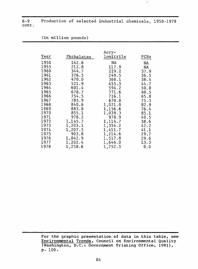
6-9 Production of selected industrial chemicals, 1950-1978
For the graphic presentation of data in this table, see Environmental Trends, Council on Environmental Quality (Washington, D.C.t Government Printing Office, 1981), p. 100.
For the graphic presentation of data in this table, see Environmenta1 Trends, Council on Environmental Quality (Washington, D.C.t Government Printing Office, 1981), p. 100 .
84
6-11 PCB residues in fish and birds, 1969-1976
(in parts per million)
Fish
Year
19691970197119721973197419751976
PCB residue
1.061.070.901.070.710.96 *0.87
Starlings
Year
1970197219741976
PCB residue
0.3580.2150.0680.243
Waterfowl
Year
196919721976
PCB residue, by flyway
Pacific Central
0.200.110.16
0.200.100.15
Missis sippi
0.440.660.23
Atlantic
1.291.240.52
*Not measured in 1975.
For the graphic presentation of data in this table, see Environmental Trends, Council on Environmental Quality (Washington, D.C.i Government Printing Office, 1981), p. 102.
85
6-12 PCB residues in human tissue, 1972-1976
(in percent of population with PCB residues detected)
Percent of population with PCB residues
Year detected
1972 74.01973 78.61974 90.71975 94.41976 98.1
For the graphic presentation of data in this table, see Environmenta1 Trends, Council on Environmental Quality (Washington, D.C.t Government Printing Office, 1981), p. 102.
86
6-13 Cancer deaths associated with vinyl chloride and poly- vinyl chloride, 1942-1973
(in standardized mortality ratio*)
Vinyl chloride workers
Standardized Type of cancer mortality ratio
All cancer 149Respiratory cancer 156Biliary and liver cancer 1155
Polyvinyl chloride communities
Standardized Type of cancer mortality ratio
Central nervous system 158
*The ratio of the number of observed to expected cancer deaths times 100.
For the graphic presentation of data in this table, see Environmental Trends, Council on Environmental Quality (Washington, D.C.i Government Printing Office, 1981), p. 103.
87
6-14 Cancer deaths associated with asbestos, 1959-1977
(in standardized mortality ratio*)
U.S. and Canadian asbestos insulation workers
Standardized Type of cancer mortality ratio
All cancer 311Lung cancer 458Esophagus cancer 257
U.S. asbestos production and textile workers
Standardized Type of cancer mortality ratio
All cancer 259Lung cancer 417Gastrointestinal cancer 260
*The ratio of the number of observed to expected cancer deaths times 100.
For the graphic presentation of data in this table, see Environmental Trends, Council on Environmental Quality (Washington, D.C.t Government Printing Office, 1981), p. 104 .
88
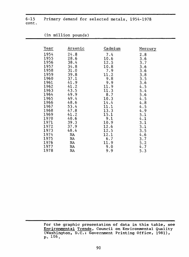
6-15 Primary demand for selected metals, 1954-1978
For the graphic presentation of data in this table, see Environmental Trends, Council on Environmental Quality (Washington, D.C.i Government Printing Office, 1981), p. 106.
For the graphic presentation of data in this table, see Environmental Trends, Council on Environmental Quality (Washington, D.C.t Government Printing Office, 1981), p. 106.
90
6-17 Cancer deaths associated with metals, 1940-1973
(in standardized mortality ratio*)
Standardized Type of cancer mortality ratio
Respiratory cancer amongcadmium smelter workers 235
Digestive organ cancer amonglead smelter workers 150
Respiratory cancer amonglead smelter workers 148
Respiratory cancer amonglead battery plant workers 132
Respiratory cancer amongarsenic workers 267
*The ratio of the number of observed to expected cancer deaths times 100.
For the graphic presentation of data in this table, see Environmental Trends, Council on Environmental Quality (Washington, D.C.t Government Printing Office, 1981), p. 108.
91
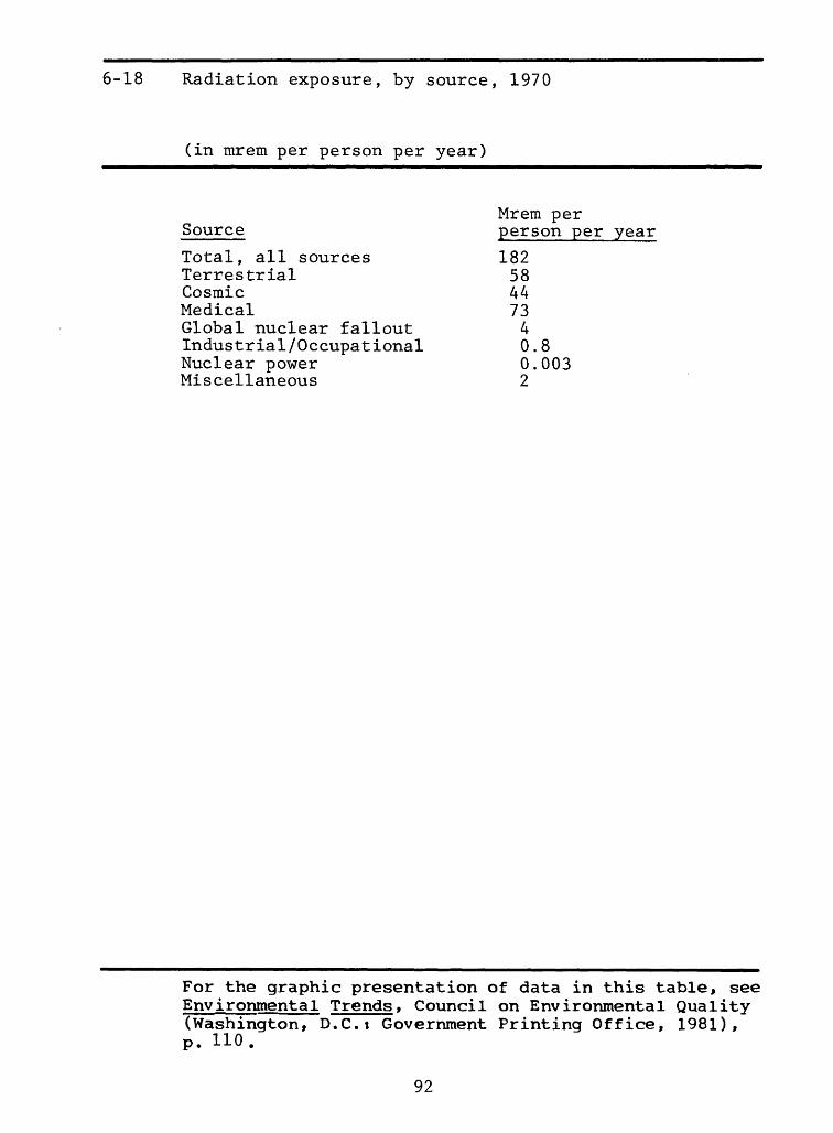
6-18 Radiation exposure, by source, 1970
(in mrem per person per year)
Mrem per Source person per year
Total, all sources 182Terrestrial 58Cosmic 44Medical 73Global nuclear fallout 4Industrial/Occupational 0.8Nuclear power 0.003Miscellaneous 2
For the graphic presentation of data in this table, see Environmental Trends, Council on Environmental Quality (Washington, D.C.i Government Printing Office, 1981), p. HO.
92
6-19 Radiation levels from nuclear fallout, as measured by strontium-90 and cesium-137 in pasteurized milk, 1960- 1978
For the graphic presentation of data in this table, see Environmental Trends, Council on Environmental Quality (Washington, D.C.t Government Printing Office, 1981), p. 112.
93
6-20 Radiation levels from nuclear power generation, as measured by krypton-85 in air, 1962-1976
For the graphic presentation of data in this table, see Environmental Trends, Council on Environmental Quality (Washington, D.C.t Government Printing Office, 1981), p. 112.
94
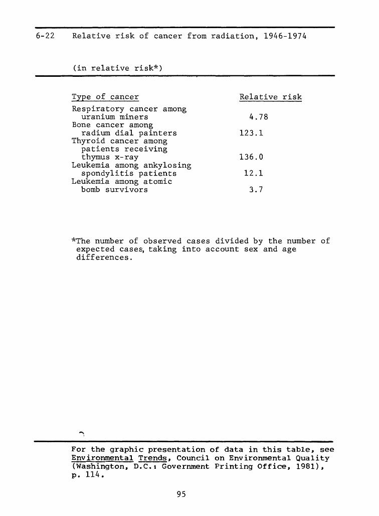
6-22 Relative risk of cancer from radiation, 1946-1974
(in relative risk*)
Type of cancer Relative risk
Respiratory cancer amonguranium miners 4.78
Bone cancer amongradium dial painters 123.1
Thyroid cancer amongpatients receivingthymus x-ray 136.0
Leukemia among ankylosingspondylitis patients 12.1
Leukemia among atomicbomb survivors 3.7
*The number of observed cases divided by the number of expected cases, taking into account sex and age differences.
For the graphic presentation of data in this table, see Environmental Trends, Council on Environmental Quality (Washington, D.C.t Government Printing Office, 1981), p. 114.
95
Chapter 7 CROPLAND, FOREST, AND RANGELAKD
96
7-2 Uses of cropland, 1949-1978
(in million acres)
Year
1949195419591964196919741975197619771978
Year
1949195419591964196919741975197619771978
Totalcropland
478465457444472465NANANA473
Summerfallow
26283137413130303031
Harvested
352339317292286322330331337330
Idle
221933525121NANANA29
Failedcrops
9131066869
107
Pasture
696666578883NANANA76
For the graphic presentation of data in this table, see Environmental Trends, Council on Environmental Quality (Washington, D.C.i Government Printing Office, 1981), p. 119.
For the graphic presentation of data in this table, see Envjronmenta1 Trends, Council on Environmental Quality (Washington, D.C.i Government Printing Office, 1981), p. 121.
For the graphic presentation of data in this table, see Envjronmenta1 Trends, Council on Environmental Quality (Washington, D.C.i Government Printing Office, 1981), p. 122.
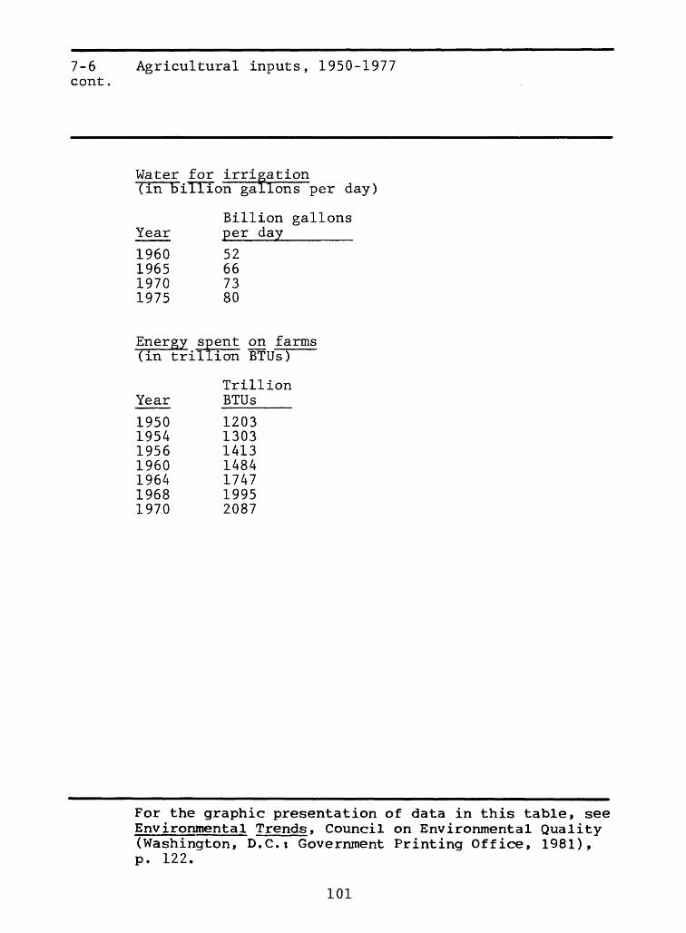
For the graphic presentation of data in this table, see Environmental Trends, Council on Environmental Quality (Washington, D.C.: Government Printing Office, 1981), p. 122.
101
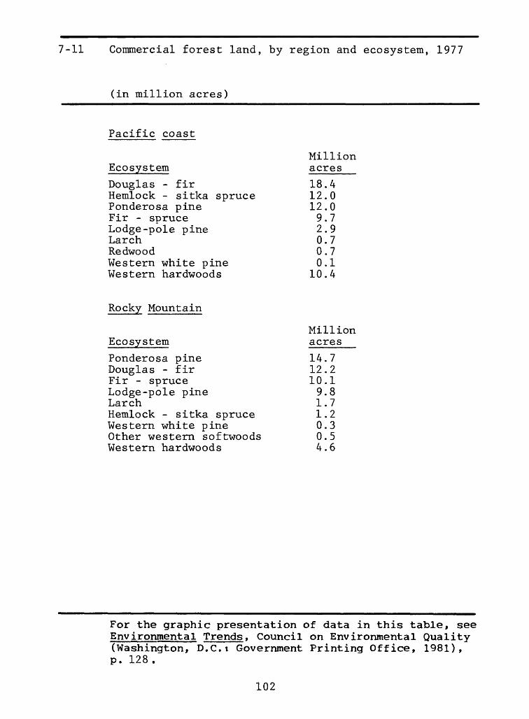
7-11 Commercial forest land, by region and ecosystem, 1977
(in million acres)
Pacific coast
Ecosystem
Douglas - firHemlock - sitka sprucePonderosa pineFir - spruceLodge-pole pineLarchRedwoodWestern white pineWestern hardwoods
Million acres
18.412.012.09.72.9
0.1 10.4
Rocky Mountain
Ecosystem
Ponderosa pine Douglas - fir Fir - spruce Lodge-pole pine LarchHemlock - sitka spruce Western white pine Other western softwoods Western hardwoods
Million acres
14.712.210.19.81.71.20.30.54.6
For the graphic presentation of data in this table, see Environmenta1 Trends, Council on Environmental Quality (Washington, D.C.t Government Printing Office, 1981), p. 128.
102
7-11 cont.
Commercial forest land, by region and ecosystem, 1977
(in million acres)
North
Million Ecosystem acres
Spruce - fir 18.3White - red - jack 11.9Loblolly - shortleaf pine 3.4Oak - hickory 51.8Maple - beech - birch 32.5Elm - ash - cottonwoods 21.9Aspen - birch 19.6Oak - pine 4.2Oak - gum - cypress 0.8
South
Million Ecosystem acres
Loblolly - shortleaf pine 46.5Longleaf - slash pine 17.0White - red - jack pine 0.4Oak - hickory 59.0Oak - pine 30.4Oak - gum - cypress 26.1Elm - ash - cottonwood 3.4Maple - beech - birch 0.4
For the graphic presentation of data in this table, see Environmental Trends, Council on Environmental Quality (Washington, D.C.t Government Printing Office, 1981), p. 128.
103
7-12 Sawtimber growth and harvest, by type, 1952-1976
(in billion board feet per year)
Total U.S.
Year
1952196219701976
Growth
45.054.265.073.6
Harvest
52.251.462.566.2
Softwood
Year
1952196219701976
Growth
29.436.043.249.1
Harvest
39.138.747.151.7
Hardwood
Yeat Growth
15.618.121.824.3
Harvest
13.012.715.414.5
For the graphic presentation of data in this table, see Environmenta1 Trends, Council on Environmental Quality (Washington, D.C.i Government Printing Office, 1981), p. 130.
104
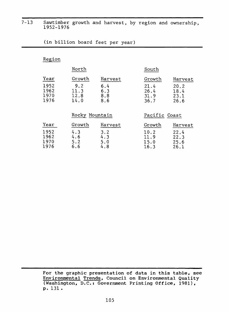
7-13 Sawtimber growth and harvest, by region and ownership, 1952-1976
(in billion board feet per year)
Region
Year
North
Growth
9.211.312.814.0
Harvest
6.4 6.3 8.8 8.6
South
Growth
21.426.431.936.7
Harvest
20.218.423.126.6
Year
1952196219701976
Rocky Mountain
Growth Harvest
Pacific Coast
4.3 4.6 5.2 6.6
3.2 4.3 5.0 4.8
Growth
10.2 11.9 15.0 16.3
Harvest
22.4 22.3 25.6 26.1
For the graphic presentation of data in this table, see Environmental Trends, Council on Environmental Quality (Washington, D.C.t Government Printing Office, 1981), p. 131 .
105
7-13 Sawtimber growth and harvest, by region and ownership, cont. 1952-1976
(in billion board feet per year)
Ownership
Year
1952196219701976
Farm and other private
Growth
23.8 28.6 34.3 39.6
Harvest
25.5 22.2 25.7 26.5
Forest industry
Growth Harvest
9.511.313.614.5
17.214.518.521.3
National forest
Year Growth
7.79.2
11.312.7
Harvest
6.711.013.412.5
Other public
Growth Harvest
4.0 5.0 5.8 6.8
2.7 3.6 4.9 5.8
For the graphic presentation of data in this table, see Environmental Trends, Council on Environmental Quality (Washington, D.C.t Government Printing Office, 1981), p. 131.
106
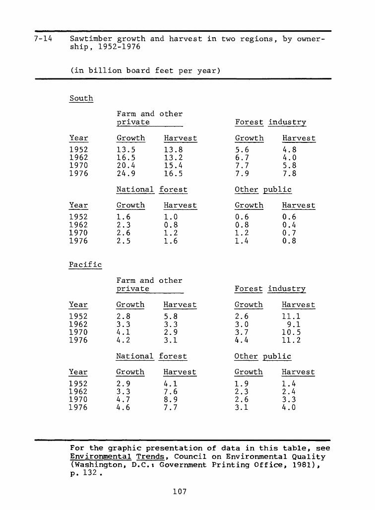
7-14 Sawtimber growth and harvest in two regions, by owner ship, 1952-1976
(in billion board feet per year)
South
Year
1952196219701976
Year
1952196219701976
Pacific
Year
1952196219701976
Year
1952196219701976
Farm andprivate
Growth
13.516.520.424.9
National
Growth
1.62.32.62.5
Farm andprivate
Growth
2.83.34.14.2
National
Growth
2.93.34.74.6
other
Harvest
13.813.215.416.5
forest
Harvest
1.00.81.21.6
other
Harvest
5.83.32.93.1
forest
Harvest
4.17.68.97.7
Forest industry
Growth Harvest
5.6 4.86.7 4.07.7 5.87.9 7.8
Other public
Gr owt h Har ve s t
0.6 0.60.8 0.41.2 0.71.4 0.8
Forest industry
Growth Harvest
2.6 11.13.0 9.13.7 10.54.4 11.2
Other public
Growth Harvest
1.9 1.42.3 2.42.6 3.33.1 4.0
For the graphic presentation of data in this table, see Environmental Trends, Council on Environmental Quality (Washington, D.C.: Government Printing Office, 1981), p. 132 .
For the graphic presentation of data in this table, see Environmental Trends, Council on Environmental Quality (Washington, D.C.t Government Printing Office, 1981), p. 133 .
For the graphic presentation of data in this table, see Environmental Trends, Council on Environmental Quality (Washington, D.C.t Government Printing Office, 1981), p. 133 .
109
7-16 Forest conditions, 1950-1978
(in million acres per year)
Area planted and direct seeded
Year
1950195119521953195419551956195719581959
Millionacres
0.490.450.520.710.810.780.891.141.532.12
Year
1960196119621963196419651966196719681969
Millionacres
2.101.761.371.331.311.291.281.371.441.43
Year
197019711972197319741975197619771978
Millionacres
1.581.691.681.751.601.931.891.982.09
Wildfire damage
Year
1950195119521953195419551956195719581959
Million acres
15.510.814.210.08.88.16.63.43.34.2
YearMillion acres
4.5 3.0 4.1 7.1 4.2 2.74.64.7 4.2 6.7
Year
19701971197219731974197519761977
Million acres
3.3 4.3 2.6 1.9 2.9 1.8 5.1 3.2
For the graphic presentation of data in this table, see Environmental Trends, Council on Environmental Quality (Washington, D.C.» Government Printing Office, 1981), p. 134.
110
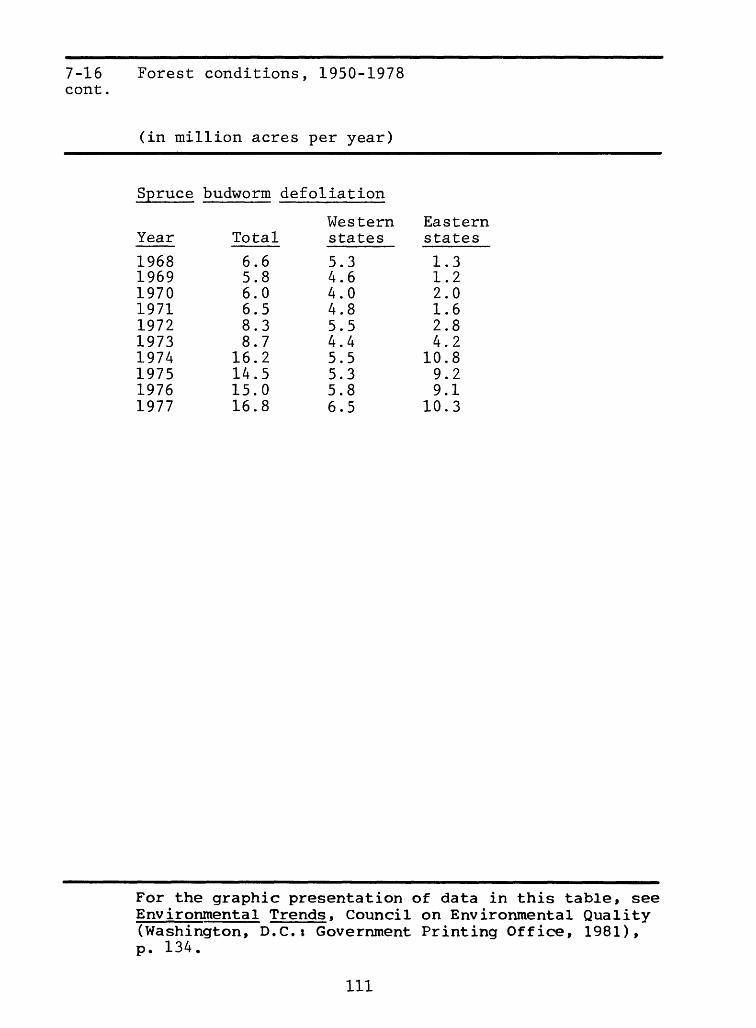
7-16 cont.
Forest conditions, 1950-1978
(in million acres per year)
Spruce budworm defoliation
Year
1968196919701971197219731974197519761977
Total
6.6 5.8 6.0 6.5 8.3 8.7
16.214.515.016.8
Western states
5.3 4.6 4.0 4.8 5.5 4.4 5.5 5.3 5.8 6.5
Eastern states
1.31.22.01.62.84.2
10.89.29.1
10.3
For the graphic presentation of data in this table, see Environmental Trends, Council on Environmental Quality (Washington, D.C.t Government Printing Office, 1981), p. 134.
Ill
7-17 Recreational use of the National Forests, 1965-1977
For the graphic presentation of data in this table, see Environmental Trends, Council on Environmental Quality (Washington, D.C.» Government Printing Office, 1981), p. 135.
112
7-18 Recreational use of the National Forests, by activity, 1977
(in million recreation visitor-days)
Recreation Million recreationactivity visitor-days_____
Camp ing 56.5Mechanized recreation travel 49.3Fishing 16.0Hunting 14.5Resort and residence use 11.0Nature study 11.0Boating and other water sports 10.4Hiking and mountain climbing 10.3Picnicing 8.3Winter sports 8.1 Visitor information
For the graphic presentation of data in this table, see Environmental Trends, Council on Environmental Quality (Washington, D.C.t Government Printing Office, 1981), p. 136.
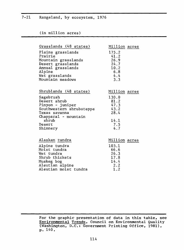
For the graphic presentation of data in this table, see Environmental Trends, Council on Environmental Quality (Washington, D.C.t Government Printing Office, 1981), p. 140.
114
7-22 Quality of rangeland, by ecosystem, 1976
(in percentages)
Mod. Mod. Grasslands (48 states) Low low high High
For the graphic presentation of data in this table, see Environmental Trends, Council on Environmental Quality (Washington, D.C.i Government Printing Office, 1981), p. 142.
115
7-22 Quality of rangeland, by ecosystem, 1976 cont.
Total, 48 states 16 38 31 15Total, 50 states 12 28 28 32
For the graphic presentation of data in this table, see Environmental Trends, Council on Environmental Quality (Washington, D.C.t Government Printing Office, 1981), p. 142.
116
7-23 Productivity of rangeland, by ecosystem, 1976
(in average pounds of herbage and browse produced per acre per year)
For the graphic presentation of data in this table, see Environmental Trends, Council on Environmental Quality (Washington, D.C.: Government Printing Office, 1981),p. 144 .
117
Chapter 8 WILDLIFE
118
8-2 Selected large mammal populations on Bureau of Land Management lands, 1961-1975
For the graphic presentation of data in this table, see Environmental Trends, Council on Environmental Quality (Washington, D.C.t Government Printing Office, 1981), p. 150.
119
8-3 Selected large mammal populations in National Forests and National Grasslands, 1960-1978
For the graphic presentation of data in this table, see Environmental Trends, Council on Environmental Quality (Washington, D.C.i Government Printing Office, 1981), p. 151 .
120
8-3 Selected large mammal populations in National Forests cont. and National Grasslands, 1960-1978
For the graphic presentation of data in this table, see Environmental Trends, Council on Environmental Quality (Washington, D.C.t Government Printing Office, 1981), p. 151.
121
8-3 Selected large mammal populations in cont. and National Grasslands, 1960-1978
For the graphic presentation of data in this table, see Environmental Trends, Council on Environmental Quality (Washington, D.C.t Government Printing Office, 1981), p. 151.
122
8-3 Selected large mammal populations in National Forests cont. and National Grasslands, 1960-1978
For the graphic presentation of data in this table, see Envi ronmenta1 Trends, Council on Environmental Quality (Washington, D.C.: Government Printing Office, 1981), p. 151.
123
8-3 Selected large mammal populations in cont. and National Grasslands, 1960-1978
For the graphic presentation of data in this table, see Environmental Trends, Council on Environmental Quality (Washington, D.C.t Government Printing Office, 1981), p. 151.
124
8-3 Selected large mammal populations in National Forests cont. and National Grasslands, 1960-1978
For the graphic presentation of data in this table, see Environmental Trends, Council on Environmental Quality (Washington, D.C.t Government Printing Office, 1981), p. 151.
125
8-4 Animals removed or killed by Federal predator control activities, 1937-1978
(in number of animals)
Year193719381939194019411942194319441945194619471948194919501951195219531954195519561957195819591960196119621963196419651966196719681969197019711972197319741975197619771978For the
For the graphic presentation of data in this table, see Environmental Trends, Council on Environmental Quality (Washington, D.C.t Government Printing Office, 1981), p. 154.
128
8-7 Most frequently observed breeding bird species, 1977
(in mean number observed per route)
Species
Red-winged blackbird House sparrow Common grackle StarlingWestern meadowlark American robin Mourning dove Common crow Eastern meadowlark Cardinal Song sparrow Barn swallow
Mean number observed per route_____
856962615836362928252422
For the graphic presentation of data in this table, see Environmental Trends, Council on Environmental Quality (Washington, D.C.t Government Printing Office, 1981), p. 155.
129
8-9 Duck breeding populations in North America, 1955-1979
For the graphic presentation of data in this table, see Environmenta1 Trends, Council on Environmental Quality (Washington, D.C.i Government Printing Office, 1981), p. 157
For the graphic presentation of data in this table, see Environmental Trends, Council on Environmental Quality (Washington, D.C.t Government Printing Office, 1981), p. 158.
131
8-11 Brown pelican populations and toxic residues in eggs, 1969-1975
(in parts per million of toxic residue in eggs)
Southern
Year
1969 19701971197219731974 1975
and Baja
DDT
1,204 NANA22118397
113
California
PCBs
200NANANA43
146 120
Number ofyoung fledged
4 5
42207134
1,185NA
South Carolina
Year
1969 1970 1971 1972 1973 1974 1975
DDT
7.81 5.27 3.20 3.69 2.56 2.72 1.80
PCBs
6.115.256.497.514.757.636.45
Dieldrin
1.160.820.460.450.450.580.40
Number ofyoungfledged
980945
1,349970
2,7261,6251,800
For the graphic presentation of data in this table, see Environmental Trends, Council on Environmental Quality (Washington, D.C.t Government Printing Office, 1981), p. 159.
132
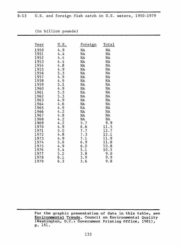
8-13 U.S. and foreign fish catch in U.S. waters, 1950-1979
For the graphic presentation of data in this table, see Environmental Trends, Council on Environmental Quality (Washington, D.C.t Government Printing Office, 1981), p. 161.
133
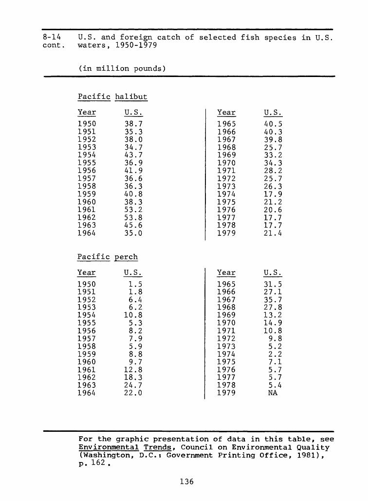
8-14 U.S. and foreign catch of selected fish species in U.S waters, 1950-1979
For the graphic presentation of data in this table, see Environmental Trends, Council on Environmental Quality (Washington, D.C.i Government Printing Office, 1981), p. 162.
134
8-14 U.S. and foreign catch of selected fish species cont. waters, 1950-1979
For the graphic presentation of data in this table, see Environmental Trends, Council on Environmental Quality (Washington, D.C.t Government Printing Office, 1981), p. 162.
135
8-14 U.S. and foreign catch of selected fish species in U.S. cont. waters, 1950-1979
For the graphic presentation of data in this table, see E nv ironment a1 Trends, Council on Environmental Quality (Washington, D.C.t Government Printing Office, 1981), p. 162.
For the graphic presentation of data in this table, see Environmental Trends, Council on Environmental Quality (Washington, D.C.i Government Printing Office, 1981), p. 165.
137
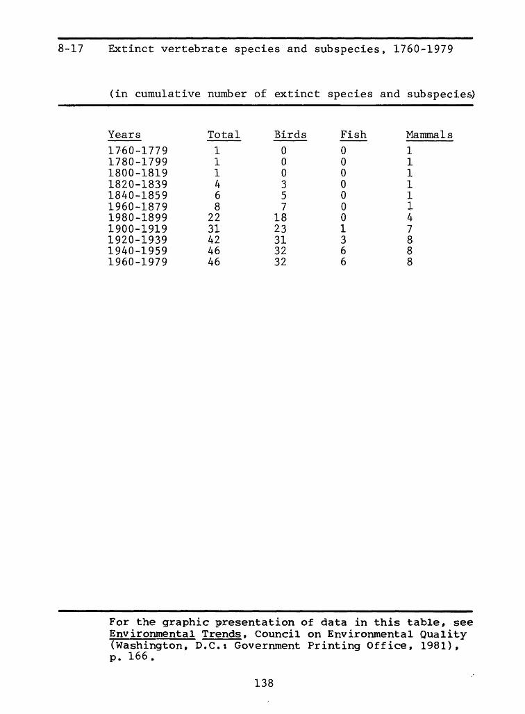
8-17 Extinct vertebrate species and subspecies, 1760-1979
(in cumulative number of extinct species and subspecies)
For the graphic presentation of data in this table, see Environmental Trends, Council on Environmental Quality (Washington, D.C.t Government Printing Office, 1981), p. 166.
138
8-18 Threatened and endangered species in the United States, December, 1979
For the graphic presentation of data in this table, see Environmental Trends, Council on Environmental Quality (Washington, D.C.t Government Printing Office, 1981), p. 167.
139
8-19 Population of selected threatened and endangered species, 1941-1979
For the graphic presentation of data in this table, see Environmental Trends, Council on Environmental Quality (Washington, D.C.t Government Printing Office, 1981), p. 168.
140
Chapter 9 ENERGY
141
9-1 Energy consumption, by fuel type, 1850-1978 and 9-2
For the graphic presentation of data in this table, see Environmental Trends, Council on Environmental Quality(Washington, D.C.t Government Printing Office, 1981), p. 177 and p. 178.
For the graphic presentation of data in this table, see Environmental Trends, Council on Environmental Quality (Washington, D.C.» Government Printing Office, 1981), p. 178.
144
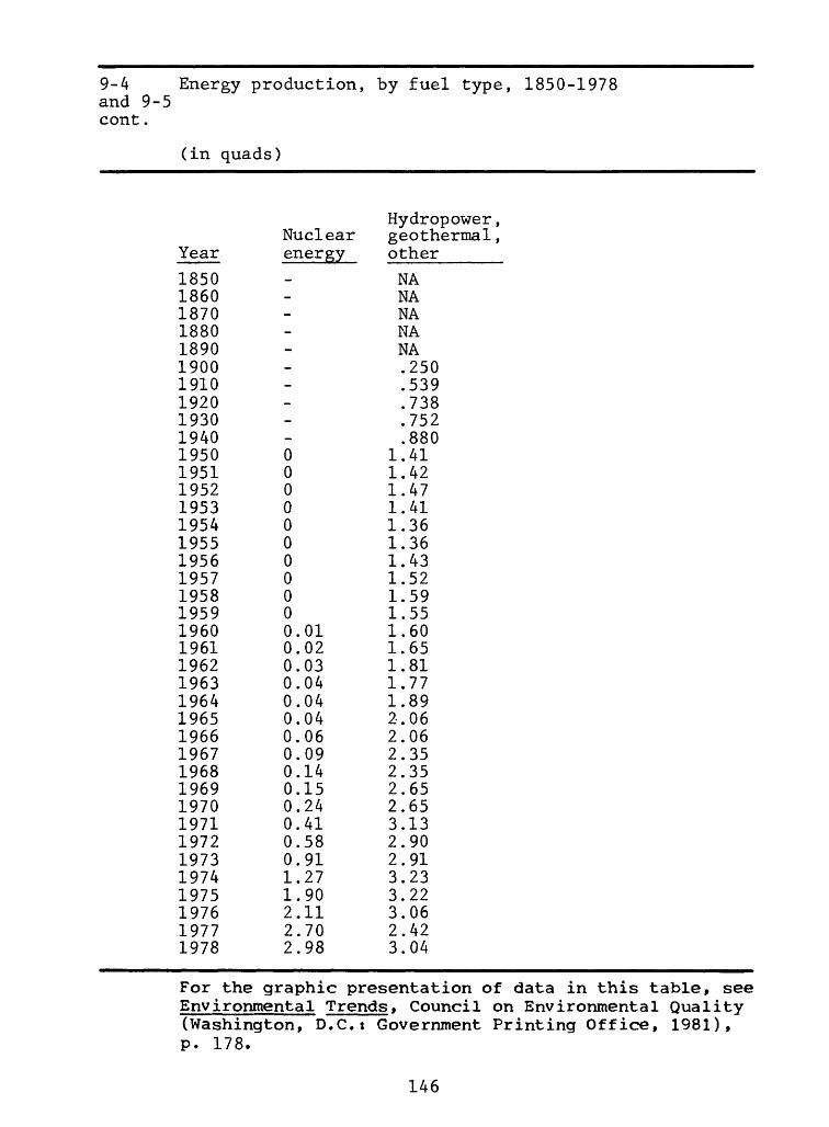
9-4 Energy production, by fuel type, 1850-1978 and 9-5
(in quads)
Total energyproduc-
Year
185018601870188018901900191019201930194019501951195219531954195519561957195819591960196119621963196419651966196719681969197019711972197319741975197619771978For the
For the graphic presentation of data in this table, seeEnvironmental Trends , Council on Environmental Quality(Washington, D.C.i Government Printing Office, 1981), p. 178.
For the graphic presentation of data in this table, see Environmental Trends, Council on Environmental Quality (Washington, D.C.i Government Printing Office, 1981), p. 182.
For the graphic presentation of data in this table, see Environmenta1 Trends, Council on Environmental Quality (Washington, D.C.t Government Printing Office, 1981), p. 183.
148
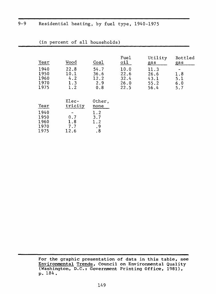
9-9 Residential heating, by fuel type, 1940-1975
(in percent of all households)
Year
19401950196019701975
Wood
22.810.14.21.31.2
Coal
54.736.612.22.90.8
Fuel oil
10.022.632.426.022.5
Utility gas
11.326.643.155.256.4
Bottled gas
1.8 5.1 6.0 5.7
Year
19401950196019701975
Elec- tricity
0.71.87.7
12.6
Other, none
1.2 3.7 1.2.9.8
For the graphic presentation of data in this table, see Environmental Trends. Council on Environmental Quality (Washington, D.C.i Government Printing Office, 1981), p. 184 .
149
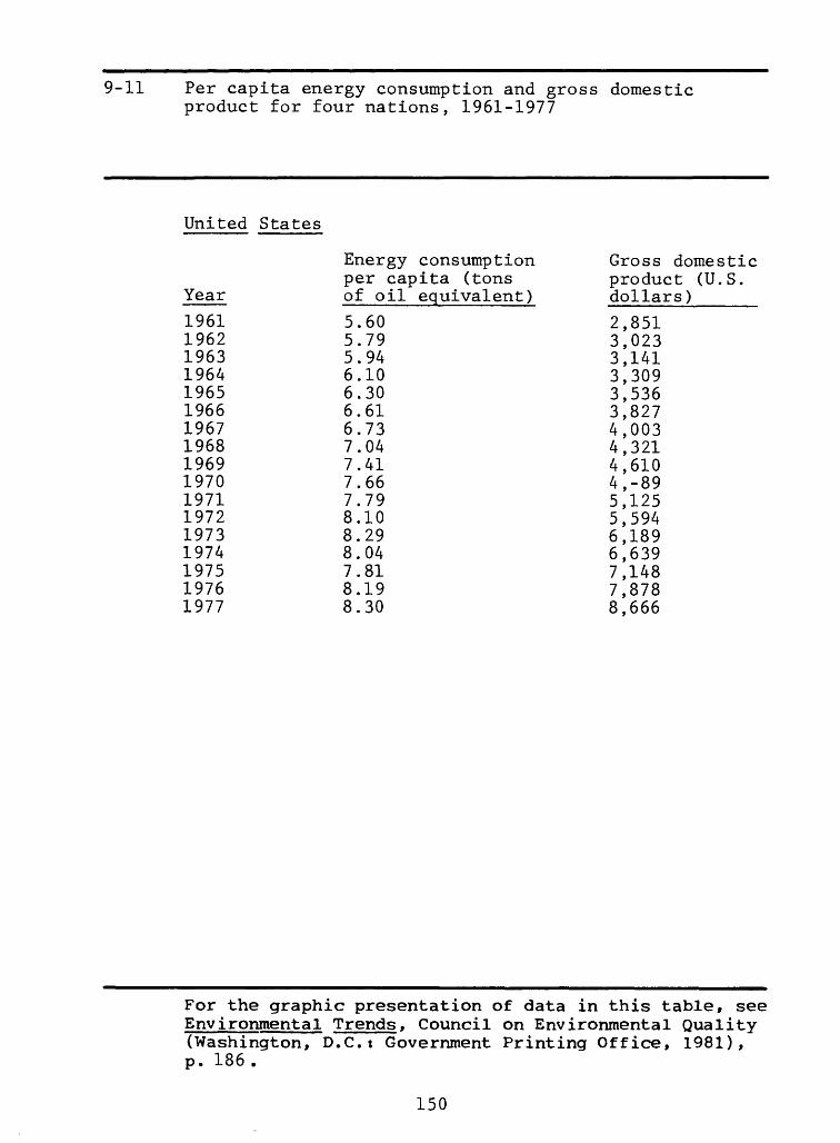
9-11 Per capita energy consumption and gross domestic product for four nations, 1961-1977
For the graphic presentation of data in this table, see Environmental Trends, Council on Environmental Quality (Washington, D.C.» Government Printing Office, 1981), p. 186 .
150
9-11 Per capita energy consumption and gross domestic cont. product for four nations, 1961-1977
For the graphic presentation of data in this table, see Environmental Trends, Council on Environmental Quality (Washington, D.C.t Government Printing Office, 1981), p. 186.
151
9-11 Per capita energy consumption and gross domestic cont. product for four nations, 1961-1977
Netherlands
Year
Energy consumption per capita (tons of oil equivalent)
1.982.172.372.442.592.682.813.103.37
7885.40.59.50
4.334.724.58
Gross domestic product (U.S. dollars)
045118
1,197388532638785950180
2,4312,8123,4304,4755,2256,0726,5377,680
For the graphic presentation of data in this table, see Environmental Trends, Council on Environmental Quality (Washington, D.C.t Government Printing Office, 1981), p. 186.
152
9-11 Per capita energy consumption and gross domestic cont. product for four nations, 1961-1977
Energy consumption per capita (tons of oil equivalent)3.203.273.393.403.553.533.523.653.75
83788500836369
Gross domestic product (U.S. dollars)
3.78
,440,498,580,709,827,936,997,873,995
2,1922,4972,8103,1683,4204,0563,9254,370
For the graphic presentation of data in this table, see Environmental Trends» Council on Environmental Quality (Washington, D.C.t Government Printing Office, 1981), p. 186 .
153
9-12 Energy consumed by sector for nine nations, 1972
(in percentage consumed by sector)
Country
Trans- porta- tion
United States 22Canada 17France 15West Germany 13Italy 15Netherlands 10United Kingdom 13Sweden 11Japan 12
Indus- trial
363339424644403151
Residen tial, commer cial , misc.
252728292432243319
Losses in generation and trans mission of electricity
172318161513232517
For the graphic presentation of data in this table, see Environmental Trends, Council on Environmental Quality (Washington, D.C.t Government Printing Office, 1981), p. 188.
of data in this table, seeon Environmental Quality
(Washington, D.C.i Government Printing Office, 1981), 191.
156
9-16 Land disturbed and reclaimed by the coal mining indus try, 1930-1978
(in million acres)
Million Status acres
Used 2.119 Reclaimed 1.545
For the graphic presentation of data in this table, see Env ironmental Trends, Council on Environmental Quality (Washington, D.C.i Government Printing Office, 1981), p. 192.
For the graphic presentation of data in this table*, see Environmenta1 Trends, Council on Environmental Quality (Washington, D.C.t Government Printing Office, 1981), p. 193.
158
9-18 Coal mine deaths from accidents, 1906-1978 cont .
For the graphic presentation of data in this table, see Envi ronmenta1 Trends, Council on Environmental Quality (Washington, D.C.: Government Printing Office, 1981), p. 193.
For the graphic presentation of data in this table, see Environmental Trends, Council on Environmental Quality (Washington, D.C.t Government Printing Office, 1981), p. 198.
161
9-23 Nuclear reactors built, being built, or planned, cont. September 1973 - December 1979
(in number of reactors)
Year and Number ofmonth reactors
July 213August 213September 212October 212November 211December 207
For the graphic presentation of data in this table, see Environmental Trends, Council on Environmental Quality (Washington, D.C.t Government Printing Office, 1981), p. 198.
For the graphic presentation of data in this table, see Environmental Trends, Council on Environmental Quality (Washington, D.C.t Government Printing Office, 1981), p. 200.
For the graphic presentation of data in this table, see Environmenta1 Trends, Council on Environmental Quality (Washington, D.C.: Government Printing Office, 1981), p. 201.
For the graphic presentation of data in this table, see Environmental Trends, Council on Environmental Quality (Washington, D.C.t Government Printing Office, 1981), p. 203.
165
9-30 Production of electricity from geothermal resources, 1970-1978
For the graphic presentation of data in this table, see Environmental Trends, Council on Environmental Quality (Washington, D.C.t Government Printing Office, 1981), p. 205.
For the graphic presentation of data in this table, see Environmental Trends, Council on Environmental Quality (Washington, D.C.t Government Printing Office, 1981), p. 206 .
For the graphic presentation of data in this table, see Env ironmental Trends > Council on Environmental Quality (Washington, D.C.i Government Printing Office, 1981), p. 219.
169
10-11 Water withdrawal, by use, 1950-1975
(in billion gallons per day)
Year
Steamelectricutilities
4072
100130170190
Irrigation
110110110120130140
Industrial and misc.
373938464744
YearPublic water supplies___
141721242729
Rural domestic
3.6 3.6 3.6 4.0 4.5 4.9
For the graphic presentation of data in this table, see Environmental Trends, Council on Environmental Quality (Washington, D.C.t Government Printing Office, 1981), p. 220.
170
10-12 Water consumption, by use, 1960-1975
(in billion gallons per day)
Year
1960196519701975
Steamelectric Irriga-utilities tion
0.2 0.4 0.8 1.9
52667380
Indus- trial and misc.
3.0 3.44.14.2
Publicwatersupplies
3.5 5.2 5.9 6.7
Rural domestic
2.8 3.2 3.4 3.4
For the graphic presentation of data in this table, see Environmenta1 Trends, Council on Environmental Quality (Washington, D.C.t Government Printing Office, 1981), p. 221.
171
10-13 Water withdrawal and consumption in the Pacific North west and California regions, 1960-1975
For the graphic presentation of data in this table, see Environmental Trends, Council on Environmental Quality (Washington, D.C.t Government Printing Office, 1981), p. 222.
172
10-14 Water withdrawal and consumption in the Great Basin, Upper Colorado, and Lower Colorado regions, 1960-1975
(in billion gallons per day)
Great Basin
Year
1960196519701975
Withdrawal
7.0 6.9 6.7 6.9
Upper Colorado
Year Withdrawal
NA 6.7 8.1 4.1
Lower Colorado
Year Withdrawal
NA 6.6 7.2 8.5
Consumption
3.3 3.0 3.2 3.6
Consumption
NA 3.3 4.1 1.7
ConsumptionNA 3.3 5.0 6.3
For the graphic presentation of data in this table, see Environmental Trends, Council on Environmental Quality (Washington, D.C.t Government Printing Office, 1981), p. 224.
173
10-15 Water withdrawal and consumption in the Missouri,Arkansas - White - Red, Rio Grande, and Texas - Gulf regions, 1960-1975
(in billion gallons per day)
Missouri
Year
1960 1965 1970 1975
Withdrawal
21.6 20.8 24.0 35.0
Consumption
7.6 10.2 12.0 15.0
Arkansas - White - Red
Year
1960 1965 1970 1975
Rio Grande
Year
1960 1965 1970 1975
Texas - Gulf
Year
1960 1965 1970 1975
Withdrawal
10.4 10.4 12.0 15.0
Withdrawal
NA 7.3 6.3 5.4
Withdrawal
NA 16.0 21.0 22.0
Consumption
4.1 5.7 6.8 9.0
Consumption
NA 4.2 3.3 3.5
Consumption
NA 7.3 6.2 8.0
For the graphic presentation of data in this table, see Environmental Trends, Council on Environmental Quality (Washington, D.C.t Government Printing Office, 1981), p. 226.
174
10-16 Water withdrawal and consumption in the Sour is - Red Rainy, Upper Mississippi, and Lower Mississippi regions, 1960-1975
(in billion gallons per day)
Souris - Red - Rainy
WithdrawalYear
0.170.300.320.36
Consumption
0.0540.0700.0710.094
Upper Mississippi
Year Withdrawal
1960196519701975
11.016.016.019.0
Consumption
0.570.730.760.80
Lower Mississippi
Year Withdrawal
1960196519701975
5.35.2
13.016.0
Consumption
1.3 2.0 3.6 5.5
For the graphic presentation of data in this table, see Environmental Trends, Council on Environmental Quality (Washington, D.C.i Government Printing Office, 1981), p. 228.
175
10-17 Water withdrawal and consumption in the Great Lakes, Ohio, and Tennessee regions, 1960-1975
(in billion gallons per day)
Great Lakes
Year
1960196519701975
Withdrawal
29.033.039.036.0
Consumption
0.931.11.2 1.1
Ohio
Year
1960196519701975
Withdrawal
24.030.036.036.0
Consumption
0.800.940.921.2
Tennessee
Year
1960196519701975
Withdrawal
7.58.27.9
11.0
Consumption
0.400.400.240.28
For the graphic presentation of data in this table, see Environmental Trends, Council on Environmental Quality (Washington, D.C.t Government Printing Office, 1981), p. 230.
176
10-18 Water withdrawal and consumption in the New England, Mid-Atlantic, and South-Atlantic - Gulf regions, 1960 1975
(in billion gallons per day)
New England
Year
1960196519701975
Withdrawal
6.47.29.7
14.0
Consumption0.290.360.410.44
Mid-Atlantic
Year Withdrawal
27.133.645.052.0
Consumption
1.2 1.5 1.4 1.6
South-Atlantic - Gulf
Year
1960196519701975
Withdrawal
18.928.435.043.0
Consumption
2.0 2.7 3.3 3.7
For the graphic presentation of data in this table, see Environmental Trends, Council on Environmental Quality (Washington, D.C.t Government Printing Office, 1981), p. 232.
177
10-19 Water withdrawal and consumption in Alaska, Hawaii, and Caribbean regions, 1960-1975
(in billion gallons per day)
Alaska
Year
1960196519701975
Withdrawal
0.200.100.250.20
Consumption
0.00070.010.0160.0056
Hawaii
Year
1960196519701975
Withdrawal
1.6 2.0 2.7 2.5
Consumption
0.410.580.810.56
Caribbean
Year
1960196519701975
Withdrawal
1.2 1.7 3.0 4.1
Consumption
0.280.270.170.24
For the graphic presentation of data in this table, see Environmental Trends, Council on Environmental Quality (Washington, D.C.j Government Printing Office, 1981), p. 234.
178
Chapter 11 WATER QUALITY
179
11-2 Fecal coliform bacteria, average annual violation rates, 1975-1979
(in violation rate, the average annual percentage of samples in violation)
Violation Year rate____
3632343535
For the graphic presentation of data in this table, see Environmental Trends, Council on Environmental Quality (Washington, D.C.t Government Printing Office, 1981), p. 240.
180
11-4 Fecal coliform bacteria in major rivers, 1966-1978
(in violation rate, the average annual percentage of samples in violation)
For the graphic presentation of data in this table, see Environmental Trends, Council on Environmental Quality (Washington, D.C.t Government Printing Office, 1981), p. 242.
181
11-4 Fecal coliform bacteria in major rivers, 1966-1978
(in violation rate, the average annual percentage of samples in violation)
Year Ohio
NA NA 79 70 67 79 65 59 51 59 46 NA NA
Dela- ware
NA 86 64 68 39 64 68 77 77 39 37 48 38
Ala bama
NA NA NA NA NA NA NA NA NA 46 NA NA NA
For the graphic presentation of data in this table, see Environmental Trends, Council on Environmental Quality (Washington, D.C.t Government Printing Office, 1981), p. 242.
182
11-5 Dissolved oxygen, average annual violation rates, 1975 1979
(in violation rate, the average annual percentage of samples in violation)
Violation Year rate____
1975 51976 61977 111978 51979 4
For the graphic presentation of data in this table, see Environmental Trends, Council on Environmental Quality (Washington, D.C.i Government Printing Office, 1981), p. 244.
183
11-7 Dissolved oxygen in major rivers, 1966-1978
(in violation rate, the average annual percentage of samples in violation)
For the graphic presentation of data in this table, see Environmental Trends, Council on Environmental Quality (Washington, D.C.t Government Printing Office, 1981), p. 246.
184
11-7 cont.
Dissolved oxygen in major rivers, 1966-1978
(in violation rate, the average annual percentage samples in violation)
For the graphic presentation of data in this table, see Environmental Trends, Council on Environmental Quality (Washington, D.C.t Government Printing Office, 1981), p. 246.
185
11-8 Total phosphorus, average annual violation rates, 1975 1979
(in violation rate, the average annual percentage of samples in violation)
Violation Year rate____
4747484847
For the graphic presentation of data in this table, see Environmental Trends, Council on Environmental Quality (Washington, D.C.t Government Printing Office, 1981), p. 248.
186
11-10 Total phosphorus in major rivers, 1966-1978 '
(in violation rate, the average annual percentage samples in violation)
For the graphic presentation of data in this table, see Environmental Trends, Council on Environmental Quality (Washington, D.C.t Government Printing Office, 1981), p. 250.
187
11-10 cont.
Total phosphorus in major rivers, 1966-1978
(in violation rate, the average annual percentage samples in violation)
of
Year Ohio
30385582788666745652334643
Dela ware
NA NA NA NA NA 38 30 NA 15 20 20 16 4
Ala bama
NA NA NA NA NA NA 48 32 NA84
10 NA
For the graphic presentation of data in this table, see Environmental Trends, Council on Environmental Quality (Washington, D.C.t Government Printing Office, 1981), p. 250.
188
11-12 Phenols in the upper Ohio River basin, 1968-1976
(in violation rate, the average annual percentage of samples in violation)
For the graphic presentation of data in this table, see Environmental Trends, Council on Environmental Quality (Washington, D.C.i Government Printing Office, 1981), p. 254.
189
11-13 Discharges to water, by pollutant and by point and nonpoint sources, 1977
(in percent of pollutant)
Pollutant
Total suspendedsolids
Total dissolvedsolids
Biochemical oxygendemand
Nitrogen Phosphorus Dissolved heavy metals
Point discharges
0.4
10
2796
60
Nonpoint discharges
99.6
90
73919440
For the graphic presentation of data in this table, see Environmental Trends, Council on Environmental Quality (Washington, D.C.t Government Printing Office, 1981), p. 255.
190
11-15 Population served by municipal wastewater systems, by level of treatment, 1960-1978
(in million people)
Million Degree of treatment people
1960 Secondary or better 4 Primary and advanced
primary 36 No treatment 70 Not served by wastewater
system 70
1970 Primary, secondary, andtertiary 86
No treatment 59 Not served by wastewater
system 58
1978 Tertiary 18Advanced secondary 31Secondary 56Advanced primary 26Primary 21No treatment 2 Not served by wastewater
system 66
For the graphic presentation of data in this table, see Environmental Trends, Council on Environmental Quality (Washington, D.C.i Government Printing Office, 1981), p. 258.
191
11-16 Eutrophication of U.S. lakes, 1975
(in percent of U.S. lakes)
Percent of Condition U.S. lakes
Exhibiting acceleratedeutrophication 85
Not exhibiting acceleratedeutrophication 15
Receiving some pointsource effluents 78
Not receiving point source effluents 7
Expected to improve withpoint source controls 37
Not expected to improvewith point source controls 41
For the graphic presentation of data in this table, see Environmental Trends, Council on Environmental Quality (Washington, D.C.i Government Printing Office, 1981), p. 262.
192
11-18 Toxic residues in Great Lakes fish, 1969-1976
(in parts per million)
Mercury (Lake St. Glair)
Year
19691970197119721973197419751976
DDT (Lake
Year
19691970197119721973197419751976
Walleye
NA2.83NA
1.381.181.071.030.78
Michigan)
Laketrout
NA19.1913.0011.319.968.427.505.65
Rockbass
NANANANA1.240.490.370.37
Cohosalmon
11.8214.039.857.174.483.823.252.98
Channelcatfish
NANANANA1.620.370.350.35
Bloaters
9.9409.876.244.332.091.331.270.90
Yellowperch
NANANANANA1.220.310.28
For the graphic presentation of data in this table, see Environmental Trends, Council on Environmental Quality (Washington, D.C.i Government Printing Office, 1981), p. 264.
193
11-18 cont.
Toxic residues in Great Lakes fish, 1969-1976
(in parts per million)
Dieldrin (Lake Michigan)
Year
19691970197119721973197419751976
PCBs
Year
19691970197119721973197419751976
Laketrout
NA0.270.200.200.270.300.350.30
(Lake Michigan)
Laketrout
NANANA
12.8618.9322.9122.2818.68
Cohosalmon
0.2100.120.110.130.090.100.100.08
Cohosalmon
NANANA
10.9312.1710.4510.779.21
Bloaters
0.2700.190.270.180.280.280.390.35
Bloaters
NA NA NA
5.665.245.574.544.11
For the graphic presentation of data in this table, see Environmental Trends, Council on Environmental Quality (Washington, D.C.i Government Printing Office, 1981), p. 264.
194
11-19 Ocean dumping of U.S. wastes by barge, 1951-1978
(in million tons)
Year
19511956196119661968197319741975197619771978
Total
1.73.45.87.49.8
10.910.48.98.37.48.3
Sewagesludge
NANANANA4.54.95.05.05.35.15.5
Indus -trial
NANANANA4.75.14.63.42.71.82.5
Construction
NANANANA0.61.00.80.40.30.40.2
For the graphic presentation of data in this table, see Environmental Trends, Council on Environmental Quality (Washington, D.C.i Government Printing Office, 1981), p. 266.
195
11-20 Oil spills in U.S. waters, 1971-1978
(in thousand incidents and million gallons spilled)
Year
19711972197319741975197619771978
Thousand incidents
7.58.4
11.011.910.911.712.611.8
Million gallons spilled
8.616.815.416.721.724.410.014.2
For the graphic presentation of data in this table, see Environmental Trends, Council on Environmental Quality (Washington, D.C.: Government Printing Office, 1981), n. 267.
196
Chapter 12 AIR QUALITY
197
12-3 Average Pollutant Standards Index (PSI) for 23 Standard Metropolitan Statistical Areas, 1974-1978
For the graphic presentation of data in this table, see Environmental Trends, Council on Environmental Quality (Washington, D.C.i Government Printing Office, 1981), p. 275.
198
12-4 Pollutant Standards Index (PSI) in 24 Standard Metro politan Statistical Areas, 1973-1978
(in days per year in PSI intervals)
Portland (Oregon)
Year
197319741975197619771978
Seattle
Year
197319741975197619771978
PSI = 100-200
17911970677673
- Everett
PSI = 100-200
17010568859160
PSI = 200-300
491213352
PSI = 200-300
57115542
PSI >
000000
PSI >
000000
300
300
San Francisco
Year
197319741975197619771978
PSI = 100-200
262927442421
PSI = 200-300
322101
PSI >
000000
300
For the graphic presentation of data in this table, see Environmental Trends, Council on Environmental Quality (Washington, D.C.i Government Printing Office, 1981), p. 276.
199
12-4 Pollutant Standards Index (PSI) in 24 Standard Metro cont. politan Statistical Areas, 1973-1978
For the graphic presentation of data in this table, see Environmental Trends, Council on Environmental Quality (Washington, D.C.t Government Printing Office, 1981), p. 276.
200
12-4 Pollutant Standards Index (PSI) in 24 Standard Metro- cont. politan Statistical Areas, 1973-1978
(in days per year in PSI intervals)
San Diego
Year
197319741975197619771978
Salt Lake
Year
197319741975197619771978
Denver
Year
197319741975197619771978
PSI = 100-200
312645654132
City
PSI = 100-200
705354855251
PSI = 100-200
115127108149122133
PSI = 200-300
523946
PSI = 200-300
111919259
20
PSI = 200-300
514535332039
PSI >
000000
PSI >
031000
PSI >
432011
300
300
300
For the graphic presentation of data in this table, see Environmental Trends, Council on Environmental Quality (Washington, D.C.i Government Printing Office, 1981), p. 276.
201
12-4 Pollutant Standards Index cont. politan Statistical Areas
(in days per year in PS I
Houston
Year PSI = 100-200
1973 NA1974 321975 441976 521977 391978 70
Kansas City
Year PSI = 100-200
1973 211974 51975 41976 61977 171978 47
St. Louis
Year PSI = 100-200
1973 1321974 621975 1131976 1081977 901978 94
(PSI) in 24 , 1973-1978
intervals)
PSI = 200-300
NA34
121124
PSI = 200-300
400189
PSI = 200-300
414416271318
Standard Metro -
PSI > 300
NA00000
PSI > 300
000000
PSI > 300
0101607
For the graphic presentation of data in this table, see Environmental Trends, Council on Environmental Quality (Washington, D.C.t Government Printing Office, 1981), p. 276.
202
12-4 Pollutant Standards Index (PSI) in 24 Standard Metro- cent, politan Statistical Areas, 1973-1978
(in days per year in PSI intervals)
Milwaukee
Year PSI = 100-200 PSI = 200-300 PSI > 300
1973 NA NA NA1974 25 4 01975 32 8 01976 24 8 01977 26 7 01978 31 3 0
Memphis
Year PSI = 100-200 PSI = 200-300 PSI > 300
Chicago
Year
197319741975197619771978
NA2210241934
PSI = 100-200
18922316467
123119
NA47023
PSI = 200-300
341528131828
NA02010
PSI > 300
123113
For the graphic presentation of data in this table, see Environmental Trends, Council on Environmental Quality (Washington, D.C.: Government Printing Office, 1981), p. 276.
203
12-4 Pollutant Standards Index (PSI) in 24 Standard Metro- cent, politan Statistical Areas, 1973-1978
(in days per year in PSI intervals)
Louisville
Year
197319741975197619771978
Buffalo
Year
197319741975197619771978
Cincinnati
Year
197319741975197619771978
PSI = 100-200
7194
1541469086
PSI = 100-200
NA4740233720
PSI = 100-200
301018405929
PSI = 200-300
14273114138
PSI = 200-300
NA1010833
PSI = 200-300
102141
PSI >
000010
PSI >NA01000
PSI >
000000
300
300
300
For the graphic presentation of data in this table, see Environmental Trends, Council on Environmental Quality (Washington, D.C.: Government Printing Office, 1981), p. 276.
204
12-4 Pollutant Standards Index (PSI) in 24 Standard Metres cont. politan Statistical Areas, 1973-1978
(in days per year in PSI intervals)
Syracuse
Year
197319741975197619771978
Rochester
Year
197319741975197619771978
PSI = 100-200
NA3555
12
PSI = 100-200
NA32846
PSI = 200-300
NA00220
PSI - 200-300
NA00000
PSI
NA00000
PSI
NA00000
>300
> 300
Philadelphia
Year
197319741975197619771978
PSI = 100-200
NA132124806971
PSI = 200-300
NA23187
1010
PSI
NA31000
> 300
For the graphic presentation of data in this table, see Environmental Trends, Council on Environmental Quality (Washington, D.C.t Government Printing Office, 1981), p. 276.
205
12-4 Pollutant Standards Index cont. politan Statistical Areas
(in days per year in PSI
Washington, D.C.
Year PSI = 100-200
1973 1121974 521975 841976 1321977 671978 67
New York
Year PSI = 100-200
1973 NA1974 NA1975 331976 381977 1861978 160
Tampa - St. Petersburg
Year PSI = 100-200
1973 NA1974 81975 91976 51977 191978 10
(PSI) in 24 , 1973-1978
intervals)
PSI = 200-300
1422261573
PSI = 200-300
NANA2262258614
PSI = 200-300
NA11002
Standard Metro -
PSI > 300
330000
PSI > 300
NANA11410
PSI > 300
NA10000
For the graphic presentation of data in this table, see Environmental Trends, Council on Environmental Quality (Washington, D.C.i Government Printing Office, 1981), p. 276.
206
12-5 National ambient carbon monoxide concentrations, 1972 1978
(in milligrams per cubic meter)
Year
1972197319741975197619771978
Milligrams per cubic meter
6049
3.163.032.792.502.35
For the graphic presentation of data in this table, see Environmental Trends, Council on Environmental Quality (Washington, D.C.i Government Printing Office, 1981), p. 280.
207
12-6 National ambient zone concentrations, 1972-1977
For the graphic presentation of data in this table, see Environmental Trends, Council on Environmental Quality (Washington, D.C.i Government Printing Office, 1981), p. 280.
208
12-7 National ambient sulfur dioxide concentrations, 1972 1977
(in micrograms per cubic meter)
Year
197219731974197519761977
Micrograms per cubic meter
23.021.420.720.41919.4
For the graphic presentation of data in this table, see Environmental Trends, Council on Environmental Quality (Washington, D.C.t Government Printing Office, 1981), p. 281.
209
12-8 National ambient total suspended particulate concentra tions, 1972-1977
(in micrograms per cubic meter)
Year
197219731974197519761977
Micrograms per cubicmeter____
66.165.062.460.161.261.0
For the graphic presentation of data in this table, see Environmental Trends, Council on Environmental Quality (Washington, D.C.t Government Printing Office, 1981), p. 281.
For the graphic presentation of data in this table, see Environmental Trends, Council on Environmental Quality (Washington, D.C.i Government Printing Office, 1981), p. 282.
211
12-10 Ambient trace metal concentrations in 92 urban areas, 1965-1974
For the graphic presentation of data in this table, see Environmental Trends, Council on Environmental Quality (Washington, D.C.t Government Printing Office, 1981), p. 283.
For the graphic presentation of data in this table, see Environmental Trends, Council on Environmental Quality (Washington, D.C.i Government Printing Office, 1981), p. 285.
For the graphic presentation of data in this table, see Environmental Trends, Council on Environmental Quality (Washington, D.C.t Government Printing Office, 1981), p. 286.
214
12-14 Nitrogen oxide emissions, 1970-1977
(in million metric tons per year)
Year
19701971197219731974197519761977
Total19.620.221.622.321.721.022.823.1
Station ary fuel combus- tion
11.111.311.912.312.111.512.413.0
Trans-por-tation
7.4 7.9 8.7 9.0 8.6 8.6 9.4 9.2
Other
1.1
0.9 1.0 0.9
For the graphic presentation of data in this table, see Environmental Trends, Council on Environmental Quality (Washington, D.C.t Government Printing Office, 1981), p. 287.
215
12-15 Nitrogen oxide emissions from stationary fuel combus tion sources, by fuel type, 1970-1977
For the graphic presentation of data in this table, see Environmental Trends, Council on Environmental Quality (Washington, D.C.i Government Printing Office, 1981), p. 287.
216
12-16 Sulfur oxide emissions, 1970-1977
(in million metric tons per year)
Year
19701971197219731974197519761977
Total
29.828.329.630.228.426.127.227.4
Stationaryfuelcombus- Industion trial
22.621.622.023.122.120.821.922.4
6.3 5.8 6.7 6.3 5.6 4.6 4.5 4.2
Other
0.9 0.9 0.9 0.8 0.7 0.7 0.8 0.8
For the graphic presentation of data in this table, see Environmenta1 Trends, Council on Environmental Quality (Washington, D.C.t Government Printing Office, 1981), p. 288 .
217
12-17 Sulfur oxide emissions from stationary fuel combustion sources, by fuel type, 1970-1977
For the graphic presentation of data in this table, see Environmental Trends, Council on Environmental Quality (Washington, D.C.i Government Printing Office, 1981), p. 288.
218
12-18 Total suspended particulate emissions, 1970-1977
(in million metric tons per year)
Year Total
22.220.919.619.217.013.713.212.4
Indus - trial
11.911.310.610.38.96.56.25.4
Station ary fuel combus- tion
7.1 6.66.46.5 5.6 5.0 4.6 4.8
Other
3.2 3.0 2.62.42.5 2.2 2.4 2.2
For the graphic presentation of data in this table, see Environmental Trends, Council on Environmental Quality (Washington, D.C.t Government Printing Office, 1981), p. 289.
219
12-19 Total suspended particulate emissions from industrial sources, 1970-1977
(in million metric tons per year)
Year
19701971197219731974197519761977
Year
19701971197219731974197519761977
Industries ,total
11.911.310.610.38.96.56.25.4
Chemicals
0.30.20.20.20.20.20.20.2
Mineralproducts
7.87.46.96.45.53.73.22.7
Petroleum
0.10.10.10.10.10.10.10.1
Metals
2.11.91.92.11.91.41.51.3
Otherindustrialproducts
1.61.71.51.51.21.11.21.1
For the graphic presentation of data in this table, see Environmenta1 Trends, Council on Environmental Quality (Washington, D.C.i Government Printing Office, 1981), p. 289.
220
12-20 Compliance status of major stationary air pollution sources, 1975-1979
For the graphic presentation of data in this table, see Environmental Trends, Council on Environmental Quality (Washington, D.C.t Government Printing Office, 1981), p. 290.
221
12-21 Compliance status of major stationary air pollution sources, by industry, 1979
(in percentages)
In InSource compliance violation
Total, major stationarysources 88 12
Iron and steel mills 23 77Primary smelters 48 52 Coal- and oil-fired power
For the graphic presentation of data in this table, see Environmental Trends, Council on Environmental Quality (Washington, D.C.i Government Printing Office, 1981), P- 291-
222
Chapter 13 BIOSPHERE
223
13-1 World population, by region, 1800-1979
(in billion people)
Year
1800185019001950196019701979
Year
1800185019001950196019701979
Year
1800185019001950196019701979
Worldtotal
.981.31.72.53.13.74.4
Europe
.15
.21
.30
.39
.43
.46
.48
NorthAmerica
.007
.03
.08
.17
.20
.23
.24
Asiatotal
.63
.80
.931.41.72.12.6
Africa
.11
.11
.13
.22
.28
.36
.46
Oceania
.002
.002
.006
.013
.016
.019
.022
SouthAsia
NANANA.72.89
1.11.4
LatinAmerica
.02
.04
.07
.16
.22
.28
.35
EastAsia
NANANA.67.83
1.01.2
USSR
.06
.08
.13
.18
.21
.24
.26
For the graphic presentation of data in this table, see Environmental Trends, Council on Environmental Quality (Washington, D.C.t Government Printing Office, 1981), p. 296.
224
13-2 World population growth rates, by region, 1950-1979
For the graphic presentation of data in this table, see Environmental Trends, Council on Environmental Quality (Washington, D.C.i Government Printing Office, 1981), p. 298.
225
13-4 Population in urban and rural areas, by size, 1920-1975
(in billion people)
Year
1920193019401950196019701975
Year
1920193019401950196019701975
Worldtotal
1.8102.0132.2462.5023.0133.6054.028
Ruralsmall
1.5941.7301.7961.8642.0192.2332.432
Urban
.216
.283
.382
.706
.9941.3711.596
andtowns
SizeMore thanmillionpeople
NANANA.181.280.442.506
Size100,000-500,000people
NANANA.151.212.268.324
of city500,000-1 millionpeople
NANANA.072.097.124.154
of cityLess than100,000people
NANANA.302.405.537.612
For the graphic presentation of data in this table, see Environmental Trends, Council on Environmental Quality (Washington, D.C.t Government Printing Office, 1981), p. 300.
226
13-5 Ten largest cities in the world, 1975
(in million people)
Million City people
Tokyo - Yokohama 17.3 New York - NortheastNew Jersey 17.0
Mexico City 10.9Shanghai 10.9London 10.7Sao Paulo 10.0Rhein - Ruhr 9.7Los Angeles - Long Beach 9.5Buenos Aires 9.3Paris 9.2
For the graphic presentation of data in this table, see Environmental Trends, Council on Environmental Quality (Washington, D.C.t Government Printing Office, 1981), p. 301.
227
13-6 Population by region, 1950-1979, with projections to 2000
(in billion people)
Year
1950196019701979
19801985199019952000
Year
195019601970197919801985199019952000
High
4.5485.0125.5446.1426.797
LatinAmerica
.16
.22
.28
.35
.347
.432
.496
.565
.636
World
2.53.13.74.4
Med.
4.4704.8845.3405.8336.350
Europe
.39
.43
.46
.48
.483
.494
.506
.518
.530
Low
4.3844.7535.1405.5335.921
USSR
.18
.21
.24
.26
.266,279.290.300.309
Asia
1.3811.6602.0462.583
2.6432.8953.1713.4703.785
NorthAmerica
.17
.20
.23
.24
.244
.254
.263
.271
.276
Africa
.22
.28
.36
.46
.459
.531
.614
.709
.814
For the graphic presentation of data in this table, see Environmental Trends, Council on Environmental Quality (Washington, D.C.i Government Printing Office, 1981), p. 302.
228
13-8 Area and productivity of ecosystems, 1970s
Ecosystem type
Continental (total) Tropical rain forest Tropical seasonal forest Temperate evergreen forest Temperate deciduous forest Boreal forestWoodland and shrublandSavannaTemperate grassland Tundra and alpine meadow Desert scrubRock , ice , and sand Cultivated landSwamp and marsh Lake and stream
Marine (total)Open ocean Upwelling zones Continental shelfAlgal bed and reef Estuaries
Area of ecosystem (in millionsquare kilometers)
149 17.0 7.5 5.0 7.0
12.08.0
15.09.0 8.0
18.024.0 14.02.0 2.5
361332.0
0.4 26.60.6 1.4
Mean netprimary productivity (in grams of carbon persquare meter per year)
324 900 675 585 540 360270315225 65 321.5
2901,125
225
6957
225 162900 810
World total 510 144
For the graphic presentation of data in this table, see Environmental Trends, Council on Environmental Quality (Washington, D.C.i Government Printing Office, 1981), p. 306.
229
13-10 Tropical moist forests, by region and country, 1945 1978
For the graphic presentation of data in this table, see Environmental Trends, Council on Environmental Quality (Washington, D.C.t Government Printing Office, 1981), p. 308.
For the graphic presentation of data in this table, see Environmental Trends, Council on Environmental Quality (Washington, D.C.j Government Printing Office, 1981), p. 312.
231
13-13 Arable and potentially arable land, by region, 1970s
(in million hectares)
Countries Arable
United States 200.5Other major exporters* 104.0Western Europe 90.1Japan 5.7Eastern Europe 54.4USSR 232.5 People's Republic of China 127.5Latin America 136.5North Africa/Middle East 91.5Other African LDCs 160.5South Asia 207.5Southeast Asia 34.9East Asia 31.1
Potentially arable____
340.0140.0135.0
8.060.0
320.0190.0475.0130.0600.0230.065.070.0
* Canada, Republic of South Africa, Australia, Argentina
For the graphic presentation of data in this table, see Environmental Trends, Council on Environmental Quality (Washington, D.C.: Government Printing Office, 1981), p. 313.
For the graphic presentation of data in this table, see Environmenta1 Trends, Council on Environmental Quality (Washington, D.C.i Government Printing Office, 1981), p. 314.
233
13-14 World agricultural production, 1954-1978 cont.
For the graphic presentation of data in this table, see Environmental Trends, Council on Environmental Quality (Washington, D.C.i Government Printing Office, 1981), p. 314.
234
13-14 World agricultural production, 1954-1978 cont.
For the graphic presentation of data in this table, see Environmental Trends, Council on Environmental Quality (Washington, D.C.j Government Printing Office, 1981), p. 314.
For the graphic presentation of data in this table, see Environmental Trends, Council on Environmental Quality (Washington, D.C.t Government Printing Office, 1981), p. 315 .
For the graphic presentation of data in this table, see Environmenta1 Trends, Council on Environmental Quality (Washington, D.C.t Government Printing Office, 1981), p. 315 .
237
13-16 Extinct species and subspecies of vertebrate animals worldwide, 1600s - 1900s
(in number of species and subspecies*)
ProbablyKnown extinct to be by the
Century extinct year 2000
1600s 211700s 361800s 841900s 85 185
^Numbers are not cumulative.
For the graphic presentation of data in this table, see Environmental Trends, Council on Environmental Quality (Washington, D.C.i Government Printing Office, 1981), p. 318.
238
13-17 Extinction of species, by region, 1980-2000
(in number of species)
Range of possible Region extinctions by 2000
World 437,000 - 1,453,000Tropical forests 249,000 - 828,000
Latin America 100,000 - 333,000Africa 20,000 - 65,000South and Southeast Asia 129,000 - 430,000
All other habitats 188,000 - 625,000
For the graphic presentation of data in this table, see Environmental Trends, Council on Environmental Quality (Washington, D.C.i Government Printing Office, 1981), P. 319.
239
13-18 Whale exploitation, by species, pre-hunting through the 1970s
Whale ab tin dance, pre-hunting and 1970s
Virgin 1970s Percent ofstock stock virgin(in (in stock
For the graphic presentation of data in this table, see Env ironmental Trends, Council on Environmental Quality (Washington, D.C.t Government Printing Office, 1981), p. 320.
240
13-18 Whale exploitation, by species, pre-hunting through the cont. 1970s
For the graphic presentation of data in this table, see Environmental Trends, Council on Environmental Quality (Washington, D.C.t Government Printing Office, 1981),p. 320.
241
13-18 Whale exploitation, by species, pre-hunting through the cont. 1970s
For the graphic presentation of data in this table, see Environmenta1 Trends, Council on Environmental Quality (Washington, D.C.t Government Printing Office, 1981), p. 320.
242
13-18 Whale exploitation, by species, pre-hunting through the cont. 1970s
For the graphic presentation of data in this table, see Environmental Trends, Council on Environmental Quality (Washington, D.C.i Government Printing Office, 1981),p. 320-
243
13-18 Whale exploitation, by species, pre-hunting through cont. the 1970s
For the graphic presentation of data in this table, see Environmental Trends, Council on Environmental Quality (Washington, D.C.t Government Printing Office, 1981),p. 320.
244
13-19 Population of selected endangered and threatened species, 1947-1979
For the graphic presentation of data in this table, see Environmental Trends, Council on Environmental Quality (Washington, D.C.t Government Printing Office, 1981), p. 322 .
245
13-19 Population of selected endangered and threatened cont. species, 1947-1979
For the graphic presentation of data in this table, see Environmenta1 Trends, Council on Environmental Quality (Washington, D.C.i Government Printing Office, 1981), p. 322.
All otherspecies21.123.525.125.927.628.930.731.432.534.936.738.337.739.442.145.547.749.952.653.055.057.359.463.464.965.367.870.471.2
For the graphic presentation of data in this table, see Environmental Trends, Council on Environmental Quality (Washington, D.C.t Government Printing Office, 1981), p. 325 .
For the graphic presentation of data in this table, see Environmental Trends, Council on Environmental Quality (Washington, D.C.: Government Printing Office, 1981), p. 328.
For the graphic presentation of data in this table, see Environmental Trends, Council on Environmental Quality (Washington, D.C.: Government Printing Office, 1981), p. 331.
249
13-24 Carbon dioxide concentrations in air, 1958-1979
For the graphic presentation of data in this table, see Environmental Trends, Council on Environmental Quality (Washington, D.C.i Government Printing Office, 1981), p. 332.
250
SOURCES AND TECHNICAL NOTES
1-1Physical characteristicsof the United States
The national atlas of the United States of America, U.S. Geological Survey (Washing ton, D.C., 1970), p. 61.
1-2Climatic zones of the United States
Climatic chart of the world, U.S. Air Force, Aeronautic Chart and Information Center (St. Louis, Mo., 1965), reprinted from World atlas: Physical, political, and economic, Edward B. Espenshade, Jr., ed. (Chicago: Rand McNally and Co., 1957). Copyright by Rand McNally and Co., R.L. 81-Y-31.
Koeppen's classification of climates is based on monthly and annual averages of temperature and precipitation. Each climatic division is designated by a series of letters. The first letter corresponds to one of five major divisions: A, rainy climates with no winters; B, dry climates; C, rainy climates with mild winters; D, rainy climates with severe winters; and E, polar climates with no warm season.
A second capital letter subdivides two of the five divisions: BS, dry grassland or steppes; BW, desert; ET, tundra; and EF, continuous frost.
Small letters are used to indicate seasonal variation in temperature and precipitation: f, moist; w, winter dry; s, summer dry; a, hot summers, temperature of warmest month is greater than 71.6°F (22°C); b, cool summers, temperature of the warmest month under 71.6°F (22°C), but with at least four months above 50°F (10°C); c, cool short summers, only one to three months above 50°F (10°C); and so forth. For further details, see An out line of geography, Preston E. James (Boston: Ginn and Company, 1943), pp. 370-379.
1-3Population distribution, 1970
Graphic summary of the 1970 population census, U.S. Bureau of the Census (Washing ton: USGPO, 1973), suppl. rep. PC(SI)-55, p. 15.
The 1970 census definition of urban popu lation includes places with 2,500 or more residents.
1-4Total population, 1900-1978,and projected to 2025
1900-1977: Statistical abstract of the United States: 1978, U.S. Bureau of the Census (Washington: USGPO, 1978), table 2, p. 6.
1978: Current population reports, U.S. Bureau of the Census (Washington: USGPO, 1978), series P-25, n. 729.
1980-2025: Current population reports (Washington: USGPO, 1977), series P-25, n. 704, table D, p. 6.
Data are as of July 1 of the year noted.Data for 1900-1978 exclude Armed Forces
overseas.Projections to 2025 include Armed Forces
overseas.
1-5Population growth rates, 1900-1978
1900-1909: Statistical abstract of the United States: 1976, U.S. Bureau of the Census (Washington: USGPO, 1976), table 2, p. 5.
1910-1969: Current population reports, U.S. Bureau of the Census (Washington: USGPO, 1973), series P-25, n. 499, tables A, 4, pp. 1, 11, in Social indicators, 1973, U.S. Office of Management and Budget (Washing ton: USGPO, 1973), pp. 246, 249.
1970-1977: Statistical abstract of the United States: 1978 (Washington: USGPO, 1978), table 2, p. 6.
1978: Current population reports (Washing ton: USGPO, 1978), series P-25, n. 729.
Rates are based on the population change during the calendar year as a percentage of the midyear population.
Prior to 1940, data exclude Alaska, Hawaii, and Armed Forces overseas, except for 1917-1919, when Armed Forces overseas were included.
Beginning in 1940, data for total U.S. population include Armed Forces overseas.
1-6Population, by region, 1950-1978
1950-1959: Current population reports, U.S. Bureau of the Census (Washington: USGPO, 1965), series P-25, n. 304, table 2, p. 10.
251
1960-1969: Current population reports (Washington: USGPO, 1971), series P-25, n. 460, table 1, p. 8.
1970-1976: Current population reports (Washington: USGPO, 1978), series P-25, n. 727, table 3, p. 7.
1977-1978: Current population reports (Washington: USGPO, 1978), series P-25, n. 790, table 1, p. 2.
1-7Population growth rates,by region, 1950-1978
See 1-6.
1-8Population density along majorcoasts, 1976
Statistical abstract of the United States: 1978, U.S. Bureau of the Census (Washing ton: USGPO, 1978), table 7, p. 10.
1-9Increase in population densityalong major coasts, 1940-1976
See 1-8.
1-10Population in urban and rural areas,1900-1950, and in metropolitanand nonmetropolitan areas, 1950-1978
Urban and rural: Historical statistics of the United States, colonial times to 1970, U.S. Bureau of the Census (Washington: USGPO, 1975), p. 12.
Metropolitan and nonmetropolitan, 1950 and 1960: Statistical abstract of the United States: 1976, U.S. Bureau of the Census (Washington: USGPO, 1976), table 15, p. 16. 1970 and 1978: Current population reports, U.S. Bureau of the Census (Washington: USGPO, 1979), series P-20, n. 336, table 19, p. 34.
Each Standard Metropolitan Statistical Area (SMSA) is divided into two areas: "central city" and "outside the central city." The largest city within each SMSA is usually designated the "central city." The remainder of the SMSA is "outside the central city." This remaining area may include cities of 50,000 or more and may be located in more than one State. Areas of the country that do not meet the SMSA criteria are designated nonmetropolitan.
In addition to the county or counties con taining such a city or cities, contiguous counties are included in an SMSA if, accord ing to certain criteria, they are socially and economically integrated with the central county. In New England, SMSAs consist of towns and cities rather than counties.
The 1950-1978 data include residents of the 243 SMSAs as defined in the 1970 Census of Population. The 1970 and 1978 data include civilian noninstitutional residents only.
1-11Metropolitan areas with populationincreases of 20% or more, 1970-1977
Current population reports, U.S. Bureau of the Census (Washington: USGPO, 1979), series P-25, n. 810, table 1, pp. 4-24.
1-12Population migration, 1970-1978
Current population reports, U.S. Bureau of the Census (Washington: USGPO, 1975), series P-20, n. 285, p. 2.
Current population reports (Washington: USGPO, 1978), series P-20, n. 331, table 1, p. 5.
Details may not add to total because of rounding.
1-13Population growth rates in metropolitanand nonmetropolitan counties, 1950-1977
1950-1970: "The new pattern of nonmetro politan population change," Calvin L. Beale and Glenn V. Fuguitt, University of Wisconsin, Center for Demography and Ecology, 1975.
1970-1977: "Trends in metropolitan and nonmetropolitan population growth since 1970," Richard L. Forstall, U.S. Bureau of the Census, 1975. Current population reports, U.S. Bureau of the Census (Washington: USGPO, 1979), series P-25, n. 810, tables 6, 7, pp. 30, 31.
1-14Population change in nonmetropolitancounties, 1970-1977
Social and economic trends in rural America, USDA Economics, Statistics, and Cooperatives Service (Washington, D.C., 1979), p. 13.
252
1-15Urban regions, 2000
Jerome P. Pickard, Appalachian Regional Commission, Washington, D.C.
Two urban regions, the Lower Rio Grande Valley and El Paso-Ciudad Juarez, are inter national and include area and population in Mexico.
2-1Natural wetlands, 1954
Water atlas of the United States, Water Information Center, Inc. (Port Washington, N.Y., 1973), plate 74.
Wetlands of the United States, Samuel P. Shaw and C. Gordon Fredine, U.S. Fish and Wildlife Service (Washington, D.C., 1956), circ. 39, plate 21.
The map does not show approximately 11 million acres of wetlands not specifically delineated.
Data not available for Alaska and Hawaii.The Fish and Wildlife Service, Office of
Biological Services, is conducting the National Wetlands Inventory. National sum mary data are expected to be available in 1982.
2-2Total wetland acreage,presettlement to 1971
Wetlands of the United States, Samuel P. Shaw and C. Gordon Fredine, U.S. Fish and Wildlife Service (Washington, D.C., 1956;, circ. 39, pp. 6-7.
"Inland wetlands: Their ecological role and environmental status," William Niermg and Richard Goodwin, Bull. Ecol. Soc. Amer. 55(2):4(June 1974).
Data include 48 States only.
2-3Wetland acreages, selected States,1850-1975
Wetlands of the United States, Samuel P. Shaw and C. Gordon Fredine, U.S. Fish and Wildlife Service (Washington, D.C., 1956), circ. 39, p. 7.
Florida State Planning Office, Tallahassee, unpublished data.
Cooperative Gulf of Mexico estuarine inventory and study, Louisiana, National Oceanic and Atmospheric Administration and Louisiana Department of Wildlife and Fisheries (New Orleans, 1971), phase I, area description, and phase IV, biology, p. 10.
"Deterioration and restoration of coastal wetlands," S. M. Gagliano et al., reprinted from Proceedings of 12th International Con ference of Coastal Engineering, Washington, D.C. (Jackson, Miss.: The Gulf Coast Associ ation of Geological Societies, 1970), p. 7.
"Versatile wetlands an endangered species," Peter Sullivan, Conservation News 41(5):20 (1976), p. 5.
Supplementary report on the coastal wetlands inventory of Delaware, U.S. Fish and Wildlife Service (Washington: USGPO, 1965).
"Search for wetlands," Kathi Jensen, Delaware Conservationist 19(16):2 (1965).
Cooperative Gulf of Mexico estuarine inventory and study, Mississippi, National Oceanic and Atmospheric Administration and Mississippi Marine Conservation Commission (Ocean Springs, Miss.: Gulf Coast Research Laboratory, 1973), pp. 16, 179, 180.
Long Island marine wetlands: Status, value, and preservation potentials, New York State Department of Environmental Conservation (Albany: Office of Planning Services, 1972), pp. 9-10.
2-4Use of filled wetlands, Maine toDelaware, 1955-1964
Fish and man: Conflict in the Atlantic estuary, John Clark (Highlands, N.J.: American Littoral Society, 1967), spec. pub. 5, reprinted in The economic and social importance of estuaries, EPA (Washington: USGPO, 1971), p. E-7.
National Wetlands Newsletter, Environ mental Law Institute, v. 1, n. 3 (February 1979).
Strengthening State wetlands regulations, U.S. Fish and Wildlife Service (Washington: USGPO, 1979).
253
"Computer-aided environmental legislative data system," U.S. Army Corps of Engineers, Construction Engineering Research Labora tory (accessed April-May 1979).
Floodplain management (Executive Order 11988) and Protection of wetlands (Executive Order 11990), both issued in May 1977, directly affect coastal and riverine wetlands by prohibiting Federal agencies from need lessly damaging or destroying floodplains and wetlands.
2-6National Wilderness PreservationSystem, 1978
USDA Forest Service.
BLM lands were first admitted to the sys tem in 1979 and are not shown on the map.
2-7Designated and proposedWilderness Areas, 1964-1979
1964-1976: USDA Forest Service, National Wilderness Monitoring System, computer printout, August 1, 1977.
1977-1979: "Wilderness fact sheet," USDA Forest Service, Recreation Manage ment Staff, February 15, 1979. Unpublished data from USDA Forest Service; National Park Service; U.S. Fish and Wildlife Service; Bureau of Land Management.
In addition to the acreage shown, the 1976 BLM Organic Act includes approximately 120 million acres which are under consideration for wilderness designation.
2-8National Wild and Scenic Rivers,1978
U.S. Department of the Interior, Heritage Conservation and Recreation Service.
2-9The National Wild and ScenicRivers System, 1968-1978
Environmental quality 1976, Council on Environmental Quality (Washington: USGPO, 1976), p. 96.
U.S. Department of the Interior, Heritage Conservation and Recreation Service, unpub lished data.
2-10The National Park System, 1979
National Park Service.
2-11National Park Service units,1872-1978
1872-1976: Index of the National Park System and affiliated areas as of January 1, 1975, National Park Service (Washington: USGPO, 1975); photocopy of updated addenda to the index, October 22, 1976.
1977: National Park statistical abstract 1977, National Park Service (Washington: USGPO, 1978), table 1, p. 1.
1978: Photocopy of updated addenda to the 1977 index, February 1979.
2-12National and State Park acreages,1872-1978
National: See 2-11.State, 1941-1975: State park Statistics-
1970, National Recreation and Park Associa tion (Arlington, Va., 1971), p. 9; Statistical abstract of the United States: 1976 (Washing ton: USGPO, 1976), table 355, p. 216; State park statistics 1975 (Arlington, Va., 1977), p. 28.
2-13Representation of natural regionsin the National Park System, 1970
Part two of the National Park System plan, natural history, National Park Service (Wash ington: USGPO, 1972), figs. 1a, 3, pp. 6-7, 12-13, based on "Physiographic divisions of the United States," N. M. Fenneman, Annals of the Association of American Geographers, v. 18(3rded., 1928).
2-14Visits to National and Stateparks, 1954-1978
National Parks, 1945-1975: Public use of the National Parks: A statistical report, 1954-1964, National Park Service (Washington: USGPO, 1966), p. 4; Public use of the National Parks: A statistical report, 1960-1970 (USGPO, 1971), p. 5; Public use of the National Parks, December 1972 (USGPO, 1972), p. 9; Public use of the National Park System, calendar year report 1973 (USGPO,
254
1974), p. 6; Public use of the National Park System, calendar year report 1975 (USGPO, 1976), p. 23. 1976: National Park statistical abstract, 1977 (USGPO, 1978), table 2, p. 2. 1977-1978: National Park statistical abstract, 1978 (USGPO, 1979), table 2, p. 2.
State Parks, 1956-1975: State park statis tics, 1970, National Park and Recreation Association (Arlington, Va., 1971), p. 9; Sfafe park statistics, 1975 (Arlington, Va., 1977), p. 27.
2-15Overnight stays in National ParkService-operated campgrounds,1960-1978
National Park statistical abstracts, 1978, National Park Service (Washington: USGPO, 1979), table 3, p. 2.
2-16The 10 most popularNational Parks, 1978
National Park statistical abstract, 1978, National Park Service (Washington: USGPO, 1979), table 4, pp. 7-17.
2-17Properties on the National Registerof Historic Places, 1968-1978
U.S. Department of the Interior, Heritage Conservation and Recreation Service, National Register of Historic Places, unpub lished data.
Includes National Historic Landmarks.
2-18Properties on the National Registerof Historic Places, by type, 1978
See 2-17.
A district may include up to 10,000 individ ual buildings or properties.
2-19Properties removed from theNational Register of Historic Places,1971-1978
See 2-17.
Excludes 22 properties removed from the register prior to 1971 and 9 properties removed with no date indicating time of removal.
2-20Urban population and lands affected by stream flooding, by Water Resources Region, 1967
Flood hazard in the United States: A research assessment, Gilbert F. White (Boulder: University of Colorado, 1975), monograph NSF-RA-E-75-006, p. 2, based on List of urban places with information about flood problems, U.S. Army Corps of Engineers (Washington, D.C., 1967) and Statistical bulle tin 317, U.S. Department of Agriculture (Washington: USGPO, 1962).
Includes approximately 4,000 large urban areas with flood problems and refers to both direct and indirect effects.
The flash flood data were developed in 1976 by the American Red Cross for the National Weather Service, U.S. Department of Commerce.
2-21Hurricane risk along the Gulfand Atlantic coasts
Hurricane hazard in the United States: A research assessment, Waltraud A. R. Brink- man (Boulder: University of Colorado, 1975), monograph NSF-RA-75-007, p. 6., based on Atlantic hurricane frequencies along the U.S. coastline, Simpson and Lawrence (Washing ton: U.S. Department of Commerce, 1971), NOAA tech. memo. NWS SR-58.
2-22Frequency of tornadoes,1953-1962
The national atlas of the United States of America, U.S. Geological Survey (Washing ton, D.C., 1975), p. 116.
Mobile home residents are particularly at risk from tornadoes. Their number increased dramatically during the 1960s, and for years the homes were not well anchored. An unanchored mobile home can be overturned by winds of 54 miles per hour; anchored mobile homes withstand winds of over 100 miles per hour. Improved construction and the use of tiedown equipment are providing more protection.
Data not available for Alaska and Hawaii.
255
2-23Earthquake risk zones
Earthquake and tsunami hazards in the United States: A research assessment, Robert S. Ayre (Boulder: University of Colo rado, 1975), monograph NSF-RA-E-75-005, p. 7, based on Disaster preparedness; Report to the Congress, Executive Office of the President, Office of Emergency Preparedness (Washington: USGPO, 1972), v. 1, 2, 3.
The map is based on the known distribution of damaging earthquakes and the modified Mercali intensities associated with these earthquakes; evidence of strain release; and consideration of major geologic structures and provinces believed to be associated with earthquake activity. The probable frequency of occurrence of damaging earthquakes in each zone was not considered in assigning ratings to the various zones.
Map revised 1969.
2-24Loss of life from selected naturaldisasters, 1900-1977
Floods, 1925-1975: Climatological data, annual summary 1977, National Oceanic and Atmospheric Administration (Asheville, N.C., 1978), 28(13): 117. 1976-1977: National Oceanic and Atmospheric Administration, National Weather Service, unpublished data.
Hurricanes, 1900-1934: Historical statistics of the United States, colonial times to 1970, U.S. Bureau of the Census (Washington: USGPO, 1975), p. 448. 1935-1977: Climato logical data, annual summary 1977, National Oceanic and Atmospheric Administration (Asheville, N.C., 1978) 28(13):77.
Tornadoes, 1916-1977: Climatological data, annual summary 1977, National Oceanic and Atmospheric Administration (Asheville, N.C., 1978), 28(13):64.
Earthquakes, 1906-1971: Earthquake and tsunami hazards in the United States: A research assessment, Robert S. Ayre (Boulder: University of Colorado, 1975), monograph NSF-RA-E-005, table I-2, p. 27. 1972-1977: National Oceanic and Atmos pheric Administration, unpublished data.
Population, 1900-1977: Statistical abstract of the United States: 1978, U.S. Bureau of the Census (Washington: USGPO, 1979), table 2, p. 6.
Average annual deaths per 10 million were calculated by dividing the average number of deaths for a given 5 years by the average annual resident population for the same period.
Lives lost, 1900-1924, are for selected years. Years reported for hurricanes are 1901, 1903, 1906, 1909, 1912, and1915-1924. For tornadoes, the years are1916-1924; for earthquakes, 1906, 1915, and 1918.
Hurricane data include North Atlantic tropical cyclones, storms that form in the tropics and that have winds of 39-73 miles per hour; hurricanes have winds of 74 miles per hour or higher accompanied by heavy rains, high waves, and tides.
Tornadoes are local storms of short dura tion formed of winds rotating at very high speeds, usually counterclockwise. These storms are visible as a vortex, a whirlpool of wind rotating about a hollow cavity in which centrifugal forces produce a partial vacuum. The fall in barometric pressure is so rapid that wooden structures are often lifted and burst open by the air confined within them.
Earthquake data include tsunamis. Earth quakes are a shaking or trembling of the earth that accompanies movement of its crust. Their magnitude is measured on a Richter scale, with the measurements increasing geometrically.
2-25Property damage from selectednatural disasters, 1900-1977
Hurricanes, 1915-1969; Hurricane hazard in the United States: A research assessment, Waltraud A. R. Brinkman (Boulder: University of Colorado, 1975), monograph NSF-RA- E-75-007, fig. 111-1, p. 23. 1970-1977: Climato logical data, annual summary 1977, National Oceanic and Atmospheric Administration (Asheville, N.C., 1978), 28(13):77.
Earthquakes, 1905-1969: Earthquake and tsunami hazards in the United States: A research assessment, Robert S. Ayre (Boulder: University of Colorado, 1975), monograph NSF-RA-E-75-005, table I-2, p. 27. 1970-1977: National Oceanic and Atmos pheric Administration, unpublished data.
256
Gross National Product, 1905-1909: Long- term economic growth, 1860-1970, U.S. Department of Commerce (Washington: USGPO, 1973), data series A1, p. 182. 1910-1939: Long-term economic growth, 1860-1970 (USGPO, 1973), data series A2, p. 183. 1940-1972: Economic report of the President: Transmitted to the Congress, February 1974, Council of Economic Advisers (Washington: USGPO, 1974), p. 250. 1973-1977: Statistical abstract of the United States: 1978, U.S. Bureau of the Census (Washington: USGPO, 1979), table 710, p. 441.
Implicit price deflator: Long-term economic growth, 1860-1970 (USGPO, 1973), data series B61 and B62, pp. 222-223. Economic report of the President: Transmitted to the Congress, February 1974 (USGPO, 1974), p. 252.
Population: Statistical abstract of the United States: 1978 (USGPO, 1979), table 710, p. 441.
Average annual property loss as a percent age of gross national product was calculated by dividing the average annual loss from the four natural hazards by the average annual gross national product for each 5 years.
For hurricanes, 1970-1977, and tornadoes, 1916-1977, property damages are reported in ranges. The midpoint of the range was used for these years.
3-1Standard Metropolitan StatisticalAreas, 1950
U.S. census of population: 1950, U.S. Bureau of the Census (Washington: USGPO, 1952), v. 1, fig. 13, p. xxxiv.
3-2Standard Metropolitan StatisticalAreas, 1978
State and metropolitan area data book, 1979, U.S. Bureau of the Census (Washington: USGPO, 1980), pp. xii-xiii.
3-3Population in suburban areasand central cities, 1940-1978
1940-1960: 7960 census of population, U.S. Bureau of the Census (Washington: USGPO, 1964), v. 1, U.S. summary, and previous decennial issues; U.S. Bureau of the Census, Population Division, unpublished data.
1970-1978: Current population reports, U.S. Bureau of the Census (Washington: USGPO, 1979), series P-20, n. 336, table 19, p. 34.
Each SMSA is divided into t'*G-areas: "central city" and "outside central city." Suburban areas here refer to outside central cities.
Population data are not strictly comparable.1940 and 1950: Resident population in 168
SMSAs as defined by the 1950 census. Excludes Alaska and Hawaii, which were admitted to the Union in 1959.
1960: Resident population in 209 SMSAs as defined by the 1960 census.
1970 and 1978: Civilian noninstitutional population in 243 SMSAs as defined by the 1970 census.
3-4Population density, by location,1940-1978
See 3-3.Density data are not strictly comparable.
See note in 3-3 for population differences.1940 and 1950: Area as defined by the
1950 census.1960 and 1970: Area as defined by the
1960 and 1970 censuses, respectively.1978: Area as defined by the 1970 census.
257
3-5Land use in Standard MetropolitanStatistical Areas, by region, 1970
Farming in the city's shadow, USDA Economic Research Service (Washington: USGPO, 1974), agr. econ. rep. 250, fig. 3, pp. 6-7.
Data refer to the average size of SMSAs in each region. Regions are USDA farm produc tion regions.
3-6Composition of housing stock, by typeof unit and location, 1977
Annual housing survey: 1977, U.S. Bureau of the Census (Washington: USGPO, 1979), part A, p. 1.
Data include 80.7 million year-round hous ing units and exclude 1.7 million vacant (seasonal and migratory) units. The annual housing survey includes the 50 States and the District of Columbia.
Single-family units are primarily detached houses. This category also includes two or more attached townhouses which are sepa rated by an unbroken ground-to-roof wall (no common basement or attic) and which have their own separate utilities.
Multifamily units consist of two or more attached units which share utilities (such as plumbing) and have no ground-to-roof wall separating them.
Mobile homes include mobile homes and trailers.
3-7Composition of housing stock,by type of unit, 1940-1977
1940: 16th census of the United States: 1940, housing, U.S. Bureau of the Census (Washington: USGPO, 1943), v. II, part 1, table 4, p. 10.
1950: Census of housing: 1950 (taken as part of the 17th decennial census of the United States) (USGPO, 1953). v. I, part 1, table 5, p. 1-3.
1960: 1960 census of housing (taken as part of the 18th decennial census of the United States (USGPO, 1963), v. I, part 1, table 5, pp. 1-16 to 1-21.
1970 and 1977: See 3-6.
3-8Occupied housing units, 1900-1977
1900-1910: Historical statistics of the United States, colonial times to 1970, U.S. Bureau of the Census (Washington: USGPO, 1975), p. 646.
1920-1970: Statistical abstract of the United States: 1978, U.S. Bureau of the Census (Washington: USGPO, 1978), table 1377, p. 792.
1977: See 3-6.
3-9Occupied housing units, per 100,000population, 1900-1977
See 3-8.
Statistical abstract of the United States: 1978, U.S. Bureau of the Census (Washing ton: USGPO, 1978), table 2, p. 6.
3-10Characteristics of new single-familyhousing units, 1966-1978
Size of house, 1966-1970: Characteristics of new one-family homes: 1974, U.S. Bureau of the Census (Washington: USGPO, 1975), constr. rep. series C25-74-13, p. 103. 1971-1975: Characteristics of new housing: 1975 (USGPO, 1976), constr. rep. series C25-75-13, p. 54. 1976-1978: Characteristics of new housing: 1978 (USGPO, 1979), constr. rep. series C25-78-13, p. 53.
Structure and facilities, 1966-1971: Char acteristics of new one-family homes: 1974, pp. 33, 39, 45, 51, 57, 75, 81. 1972-1977: Characteristics of new housing: 1977 (USGPO, 1978), constr. rep. series C25-77-13, pp. 34, 42, 43. 1978: Characteristics of new housing: 1978, pp. 32, 38, 39.
Data on size of house include new single- family houses sold, including townhouses.
Data on structure and facilities include homes sold and contractor-built, owner-built, and rental home started in 1966-1970. For 1971-1978, they include privately owned single-family houses completed.
Percentages exclude houses for which questions were not answered.
Two or more stories include split-level homes.
258
3-11Characteristics of new multifamilyhousing units, 1971-1978
1971-1973: Characteristics of new housing: 1975, U.S. Bureau of the Census (Washington: USGPO, 1976), constr. rep. series C25-75-13, table 17, pp. 42-44. 1974-1978: Characteristics of new housing: 1978 (USGPO, 1979), constr. rep. series C-25-78-13, pp. 44-46.
Data refer to privately owned multifamily units completed. Air conditioning refers to both central air conditioning and individual room units.
3-12Condition of housing, 1940-1977
1940: Social indicators, 1973, U.S. Office of Management and Budget (Washington: USGPO, 1973), pp. 206, 209, from 16th census of the United States: 1940, housing, U.S. Bureau of the Census (Washington: USGPO, 1943), v. II, part 1, pp. 16, 38.
1950-1970: Housing in the seventies, U.S. Department of Housing and Urban Develop ment (Washington: USGPO, 1973), p. 6-4, from 7970 census of housing, U.S. Bureau of the Census (Washington: USGPO, 1972), and previous decennial issues.
1977: See 3-6, pp. 2, 4.
Lacking complete plumbing, 1940: Lacking some or all basic plumbing facilities private bath, private flush toilet, running water. 1950-1970: Lacking one or more plumbing facilities or sharing a facility. 1977: Lacking some or all plumbing facilities.
Crowded: More than one person per room.Dilapidated, 1940: Needing major repair a
unit with serious defects which require repair or replacement or a unit continued neglect of which would jeopardize soundness of the structure or safety of the occupants. 1950-1970: A unit which does not provide safe and adequate shelter and endangers health, safety, or well-being of the occupants. Defects are so critical or widespread that the structure should be extensively repaired, rebuilt, or torn down.
3-13Homes with selected major electricappliances, 1950-1977
Merchandising (New York: Billboard Publi cations, 1978) and previous annual issues.
Estimates are based on appliances shipped by manufacturers, appliances, purchased from retailers (initial purchases and replace ments), and lifetime expectancies of appliances.
Percentages refer to the number of homes wired for electricity (75.8 million in 1977).
Clothes washers, 1950 and 1955: Available data are not comparable and are therefore excluded.
3-14Overall opinion of living unit,by location, 1977
See 3-6, part B, p. 8.
3-15Overall opinion of neighborhood,by location, 1977
See 3-6, part B, pp. 17-18.
3-16Inadequate neighborhood services,1973-1977
See 3-6, part B, pp. 16-17, and previous annual issues.
3-17Neighborhood deficiencies, 1973-1977
See 3-6, part B, pp. 13-15, and previous annual issues.
4-1Major transportation networks, 1925-1978
Roads, 1925-1970: Historical statistics of the United States, colonial times to 1970, U.S. Bureau of the Census (Washington: USGPO, 1975), p. 710. Highway statistics, summary to 1975, Federal Highway Administration (Washington: USGPO, 1977), p. 211. 1977: Highway statistics 1977, Federal Highway Administration (Washington: USGPO, 1979), p. 229.
259
National Interstate Highway System, 1956-1978: "Quarterly report on the Federal- aid highway program, December 31, 1978," U.S. Department of Transportation, Office of Assistant Secretary for Governmental and Public Affairs (news release, April 24, 1979, and previous issues).
Natural gas pipelines, 1960-1976: "Brief excerpts from Gas Facts," American Gas Association (Arlington, Va., 1978), p. 7.
Petroleum pipelines, 1960-1976: Statistical abstract of the United States: 1978, U.S. Bureau of the Census (Washington: USGPO, 1978), table 1128, p. 665.
Railways, 1929-1977: Yearbook of railroad facts, Association of American Railroads (Washington, D.C., 1979), p. 46.
Airways and inland waterways, 1939-1976: Transportation facts and trends (14th ed.), Transportation Association of America (Washington, D.C., 1978), p. 31.
Heavy rail transit (subway), 1945-1975: "United States rapid transit systems," Bob Abrams, National Capital Transportation Agency (Washington, D.C., 1965). U.S. Department of Transportation, Urban Mass Transit Administration, unpublished data.
All data are in statute miles.National Interstate Highway System data
are miles open at end of year.Pipeline data include natural gas transmis
sion lines and petroleum trunk lines.Railways include all line-haul railroads and
exclude yard tracks and sidings; one mile of railroad may include two or more parallel tracks.
Airways, 1960-1976, includes jet routes.Heavy rail transit data are route-miles, not
miles of track, for Atlanta, Baltimore, Boston, Chicago, Cleveland, the District of Columbia, New York City, the Trans-Hudson Port Authority and the New Jersey-Pennsylvania Port Authority, Philadelphia, and San Fran cisco.
Inland waterways are commercially navigable.
4-2Transportation vehicles,1920-1978
Autos, trucks, and buses, 1920-1975: Highway statistics, summary to 1975, Federal Highway Administration (Washington: USGPO, 1977), table MV-200, p. 45. 1976-1977: Highway statistics 1977, Federal Highway Administration (Washington: USGPO, 1979) p. 62.
Motorcycles, 1940: Statistical abstract of the United States: 1976, U.S. Bureau of the Census (Washington: USGPO, 1976), table 988, p. 593. 1950-1977: Statistical abstract of the United States: 1978 (Washington: USGPO, 1978), table 1090, p. 649.
Railroad cars, 1929-1977: Yearbook of railroad facts, Association of American Railroads (Washington, D.C., 1979), pp. 48, 49, 52.
Civil aircraft, 1929-1955: Historical statistics of the United States, colonial times to 1970, U.S. Bureau of the Census (Washington: USGPO, 1975), p. 772. 1960-1976: Statistical abstract of the United States: 1978, U.S. Bureau of the Census (Washington: USGPO, 1978), table 1131, p. 669.
Recreational boats, 1973-1976: Recrea tional boating in the continental United States in 1973 and 1976: The Nationwide Boating Survey, U.S. Coast Guard (Washington: USGPO, 1978), pp. 21, 22.
Freight vessels, 1970-1976: Transportation energy conservation data book (3rd ed.), Oak Ridge National Laboratory (Oak Ridge, Tenn., 1979), p. 1-154.
Population: Statistical abstract of the United States: 1978, U.S. Bureau of the Cen sus (Washington: USGPO, 1978), table 2, p. 6.
Autos, trucks, and buses include registered vehicles.
Motorcycles, 1940-1977, include registra tions of publicly owned motorcycles and excludes military vehicles. The 1977 data are estimated.
Railroad cars include locomotives, freight cars, and passenger cars in service.
Civil aircraft, 1950-1976, includes active and inactive aircraft, gliders, dirigibles, balloons, and blimps.
260
Recreational boats, 1973-19/6, include runabouts, rowboats, johnboats, sailboats, canoes, cabin cruisers, skiffs, dinghies, kayaks, rafts, houseboats, and other boats.
Freight vessels, 1970-1976, include towboats, tugs, and barges operated for freight transportation on U.S. waterways.
Population is the resident population.
4-3Sales of specialized vehicles,1961-1978
Motorcycles, 1972-1977: 1978 motorcycle statistical annual, Motorcycle Industry Coun cil (Washington, D.C., 1978), p. 12, and previous annual issues.
Snowmobiles: An assessment of the snowmobile manufacturing industry and sport, 1978, International Snowmobile In dustry Association (Washington, D.C., 1978), appendix A, p. 47.
Recreational vehicles, 1961-1966: Motor vehicle facts and figures 1976, Motor Vehicle Manufacturers Association (Detroit, 1977), p. 27. 1967-1977: Facts and trends 1977, Recreational Vehicle Industry Association (Chantilly, Va., 1978), p. 4. 1978: Marketing report, Recreational Vehicle Industry Associa tion (Chantilly, Va., 1979), p. 6.
Mopeds, 1975-1977: Moped Association of America, unpublished data. 1978: News release.
Motorcycles include wholesale shipments to dealers by Harley Davidson, Honda, Kawasaki, Suzuki, and Yamaha for on- highway, off-highway, and dual-purpose bikes.
Recreational vehicles include total shipments of travel trailers, truck campers, camping trailers, and motor homes, except for 1961-1964, when motor homes are ex cluded.
Snowmobiles include all North American retail sales. Year refers to model year; for ex ample, 1978 data are for April 1977 through March 1978.
4-4Local passenger travel, 1950-1975
U.S. Department of Transportation, Office of the Secretary, unpublished data, in En vironmental Quality 1977, Council on En vironmental Quality (Washington: USGPO, 1977), p. 321.
Autos include taxis and personal trucks.
4-5Principal means of transportationto work, 1960-1977
1960-1970: Residential energy uses, U.S. Bureau of the Census (Washington: USGPO, 1977) current housing reports, series H-123, special reports, chart 6.
1974-1977: Annual housing survey: 1977, U.S. Bureau of the Census (Washington: USGPO, 1979), part A, p. 6, and previous an nual issues.
Data are not strictly comparable. Data for 1960-1970 include all workers 14 years old and older; 1974-1977 data include heads of households only.
4-6Principal means of transportationto work, by location, 1977See 4-5.
4-7Intercity passenger travel,1929-1977
All modes, 1929: National transportation trends and choices, U.S. Department of Transportation (Washington: USGPO, 1977), p. 114. 1939-1959: Transportation facts and trends (13th ed.), Transportation Association of America (Washington, D.C., 1977), p. 18. All modes except air, 1960-1977: Motor vehicle facts and figures 1978, Motor Vehicle Manufacturers Association (Washington, D.C., 1978), p. 54.
Air, 1960-1977: Transportation facts and trends (14th ed.), Transportation Association of America (Washington, D.C., 1978), p. 18.
Population: Statistical abstract of the United States: 1978, U.S. Bureau of the Cen sus (Washington: USGPO, 1978), table 2, p. 6.
All 1977 data are preliminary.Autos and buses data include intracity
portions of intercity trips and excludes rural- to-rural trips, strictly intracity trips with both origin and destination in the same city, local bus or transit movement, and nonrevenue school and government bus operation.
Railroad data include commuter travel.Commercial aircraft, 1970-1977, includes
Alaska and Hawaii.Population is the resident population.
261
4-8Intercity freight transportation,1929-1977
1929: National transportation trends and choices, U.S. Department of Transportation (Washington: USGPO, 1977), p. 114.
1939-1977: Transportation facts and trends (14th ed.), Transportation Association of America (Washington, D.C., 1978), p. 8.
Data include both for-hire and private carriers and mail and express transportation as appropriate, except for railroads, 1969-1977.
4-9Major pipelines, 1975
National transportation trends and choices, appendix U.S. transportation atlas, U.S. Department of Transportation (Washington: USGPO, 1976).
4-10Energy consumption, by modeof transportation, 1965-1977
Transportation energy conservation data book (3rd ed.), Oak Ridge National Laboratory (Oak Ridge, Tenn., 1979), ORNL-5493, p. 2-13.
Energy use for recreational boats, included in the total, is not disaggregated separately. One estimate for 1976 puts this figure at 0.38 quads per year.
Highway total includes civilian autos (passenger cars and taxis), motorcycles, buses (intercity, school, and local), and trucks.
Air includes general aviation and certified air carriers.
Water transport is estimated from fuel purchased domestically.
Rail includes local rail (heavy and light) and operating Class 1 railroads (passenger and freight).
Total for all modes includes gasoline used for other purposes than highway, water, and air transportation, such as for cleaning fluid, fire starters, lawn mowers, etc.
4-11Energy intensity for freighttransportation, 1976
See 4-10, p. 2-28.
The unit of measure is the number of Btu consumed per route-ton-mile. A route-ton-mile represents one ton of goods transported one route-mile. A route-mile is the distance travel ed between two selected points, a distance that differs for transportation modes. For ex ample, the distance traveled by air is shorter than that traveled by auto or rail, so that data are not strictly comparable among modes.
Data for pipelines are not available in a comparable form.
4-12Energy intensity for local and inter city passenger travel, 1976
See 4-10, p. 2-28.
The unit of measure is the number of Btu consumed per route-passenger-mile traveled. A route-passenger-mile represents one passenger traveling one route-mile. (See 4-11.)
Data do not include energy used in con struction and maintenance.
Disaggregated local and intercity auto passenger travel data are not available.
All cars: Highway statistics 1977, Federal Highway Administration (Washington: USGPO, 1979), table VM-1, p. 100, and previous annual issues. Highway statistics, summary to 1965, Federal Highway Administration (Washington: USGPO, 1967), table VM-201A, p. 42.
New cars: Transportation energy conserva tion data book (3rd ed.), Oak Ridge National Laboratory (Oak Ridge, Tenn., 1979), ORNL-5493, p. 2-29.
Data are not strictly comparable.Data for all cars are based on the average
number of miles traveled per gallon of fuel consumed.
Data for new cars are based on the 1975 Federal Test Procedure, which is weighted to take into account both city and highway driving.
262
New cars, 1967-1974 model years, production data were used; 1975-1978 model years, manufacturers' sales forecast data were used.
4-14Automobile emissions and standards,1957-1985
All autos, 1957-1967: Statistical abstract of the United States: 1978, U.S. Bureau of the Census (Washington: USGPO, 1978), table 360, p. 216. 1970-1978: U.S. Environmental Protection Agency, unpublished data.
New autos: The costs of clean air, 1974, U.S. Environmental Protection Agency (Washington, D.C., 1974), table 3-1, p. 111-4. Automobile exhaust emission surveillance analysis of the fiscal year 1974 program, U.S. Environmental Protection Agency (Ann Arbor, Mien., 1976), p. 12. Environmental quality 1977. Council on Environmental Quality (Washington: USGPO, 1977), p. 22. U.S. Department of Commerce, Bureau of Economic Analysis, unpublished data.
Emissions from all light-duty autos, 1970-1978, and from all new autos are measured by the 1975 Federal Test Procedure, which assumes an average speed of 19.6 miles per hour at 75° F.
1957-1974: Passenger cars and light-duty trucks with a gross vehicle weight of 6,000 pounds or less.
1975-1985: Passenger cars only.Nitrogen oxides, 1957-1967: No estimates
available.
4-15Noise levels of surface transportationvehicles, 1971
Report to the President and Congress on noise, U.S. Environmental Protection Agency (Washington: USGPO, 1972), Sen. doc. 92-63, p. 2-77.
4-16Population exposed to noiseat 23 major airports, 1972
Aviation noise abatement policy, U.S. Department of Transportation, Office of the Secretary, and Federal Aviation Administra tion (Washington, D.C., 1976), p. 20.
5-1Flow of materials, products,and solid wastes, 1977
Adapted from Choices for conservation, Resource Conservation Committee (Washing ton: USGPO, 1980), fig. 1, p. 7.
Resource recovery refers to a productive use of material that would otherwise be dis posed of as waste. It encompasses recycling, material conversion, and energy recovery. The most common process is recycling, the reprocessing of wastes to recover the original raw material. For example, steel is recovered from tin cans and fiber is recovered from wastepaper. Reuse differs in that a product is reused in the same form; for example, glass bottles. In material conversion, the waste is used in a different form, such as in road- paving material from auto tires. Energy recovery refers to obtaining heat from organic wastes, as in refuse-derived fuel incinerators.
5-2U.S. material consumption,1948-1978
See 5-1, table 3, p. 28.
Estimates for the raw materials consumed account for more than 95% of all material use by weight. Only large volume materials have been included. Synthetic organics other than plastics and many metals were omitted.
5-3U.S. material consumption in relation to gross national product, 1948-1978
See 5-1, table 4, p. 29.
5-4U.S. material consumptionper capita, 1948-1978
See 5-1, table 4, p. 29.
263
5-5Solid wastes disposed of by manufactur ing industries, 1974-1977
Pollution abatement costs and expendi tures, 1977, U.S. Bureau of the Census (Washington: USGPO, 1979), current industrial reports MA-200(77)-2, table 4a, and previous annual issues.
Data include solid wastes properly disposed of by means acceptable to local, State, and Federal authorities. Recovered materials are excluded. The aggregated data are composed partly of wet weight and partly of dry weight figures. Wet weight, which includes the water content, is the tonnage actually handled and charged for by the waste treatment industry.
The apparent decline in lumber wastes between 1976 and 1977 may reflect a change in survey samples rather than a change in the amount of solid wastes disposed of.
Sludge is the residue from scrubbers or after wastewater has been treated.
Dumps, landfills, sanitary landfills, and secured landfills are the four major types of solid waste land disposal sites that receive both municipal and industrial (including com mercial) solid waste. In its Report to Con gress: Waste disposal practices and their effects on ground water (Washington: USGPO, 1977), p. 145, EPA has defined the four major types of sites as follows:
"A dump is an uncovered land disposal site where solid and/or liquid wastes are deposited with little or no regard for pollution control or aesthetics. Dumps are susceptible to open burning and are exposed to the elements, vectors, and scavengers.
"A landfill is a land disposal site located without regard to possible effects on water resources, but which employs intermittent or daily cover to minimize scavenger, aesthetic, vector, and air pollution problems.
"A sanitary landfill is a land disposal site that employs an engineered method of dis posing of solid wastes on land in a manner that minimizes environmental hazards by spreading the solid wastes in thin layers, compacting the solid wastes to the smallest practical volume, and applying and compact ing cover material at the end of each oper ating day.
"A secured landfill is a land disposal site that allows no hydraulic connection with natural waters, segregates the waste, has restricted access, and is continually moni tored."
Leachate is formed from water percolating through solid wastes. Leachate from post- consumer solid wastes is a highly mineralized fluid containing chloride, iron, lead, copper, sodium, nitrate, and a variety of organic chemicals. Municipal sites generate about 90 billion gallons of leachate per year, most of it filtering into ground water. If manufacturing wastes are included, hazardous substances such as cyanide, cadmium, chromium, chlori nated hydrocarbons, and PCBs may be present in leachate.
"USEPA's industry studies on hazardous waste management," presented at the National Conference on Hazardous Waste Management, San Francisco, February 1, 1977, table 3, p. 9.
Data on hazardous wastes by the manufac turing sector are not strictly comparable to the data on total manufacturing solid waste shown in 5-5.
EPA studied seven other industries: Special machinery, which generates 0.16 million metric tons per year; leather tanning, 0.15; paint and allied products, 0.10; pharmaceuti- cals, 0.07; waste oil re-refining, 0.06; elec tronic components, 0.04; batteries, 0.01.
Hazardous wastes can damage human health or living organisms because these wastes are lethal, nondegradable, or persistent. They can be biologically magnified. They can cause or tend to cause detrimental, cumulative effects.
EPA has defined potentially hazardous waste in terms of potential damage from improper land disposal. These damages include "ground water contamination via leachate; surface water contamination via runoff; air pollution via open burning, evapo ration, sublimation, and wind erosion; poison ing via direct contact; poisoning via the food chain; and fire and explosion." ("The poten tial for national health and environmental damages from industrial residue disposal," E. C. Lazar, et al., in Proceedings of the National Conference on Disposal of Residues on Land, September 13-15, 1976, sponsored by the EPA Office of Solid Waste, p. 196.)
5-8Consumer solid wastes disposedof and recycled, 1960-1978
1960-1970: "Post-consumer solid waste and resource recovery baseline," Franklin Associates, Ltd., prepared for the Resource Conservation Committee (Washington: EPA, 1979), table 1, p. 9.
1971-1976: Environmental Protection Agency, Office of Solid Waste, unpublished data.
1977-1978: Franklin Associates, Ltd., unpublished data prepared for the Committee.
Consumer solid wastes exclude wastewater treatment sludge (about 5 million tons, dry weight, per year), discarded autos and build ing demolition materials (30-40 million tons per year), street sweepings, and litter.
If food and yard wastes are excluded, the net waste disposed of by consumer resi dential and commercial sources in 1978 becomes 100 million tons.
The International Trade Commission pub lishes production and sales data for a synthetic organic chemical only if three or more companies produce it. Because most pesticides are patented and are produced by fewer than three companies, production data do not become public knowledge. Production data include the quantity made available by the original manufacturers only; they exclude intermediate products. About a fourth of the amount produced is exported.
National pesticide use is currently monitored for agriculture only; missing from the totals is the approximately 40% used in or around the home, in government, and in the commercial sector.
Data from quinquennial USDA farm surveys (see sources in 6-4) are made public approximately 2 years after the data are collected.
Insecticides include fumigants, rodenti- cides, and a small quantity of synthetic soil conditioners.
6-3Insecticide production, by typeof chemical, 1960-1978
Synthetic organic chemicals 1978, Interna tional Trade Commission (Washington: USGPO, 1979), and previous annual issues; organochlorine data for 1970-1976 were esti mated from a graph in the 1976 issue (USGPO, 1977), p. 268.
Insecticides include rodenticides, soil con ditioners, and fumigants. Organophosphorous data are not available for 1967-1969. Because of confidentiality rules, carbamate data are not available.
265
6-4Selected herbicides used by farmerson crops, 1964-1976
1964: Quantities of pesticides used by farmers in 1964, USDA Economic Research Service (Washington: USGPO, 1968), agr. econ. rep. 131, pp. 19, 20.
1966: Quantities of pesticides used by farmers in 1966, USDA Economic Research Service (Washington: USGPO, 1970), agr. econ. rep. 179, tables 23, 25, pp. 37, 38, 44.
1971: Farmers' use of pesticides in 1971 Quantities, USDA Economic Research Serv ice (Washington: USGPO, 1974), agr. econ. rep. 252, pp. 9, 40, 41.
1976: Farmers' use of pesticides in 1976, USDA Economics, Statistics, and Coopera tives Service (Washington: USGPO, 1978), agr. econ. rep. 418, pp. 9, 36, 38.
6-5Selected insecticides used by farmerson crops, 1964-1976
1964: Quantities of pesticides used by farmers in 1964, USDA Economic Research Service (Washington: USGPO, 1968), agr. econ. rep. 131, pp. 26, 27.
1966: Quantities of pesticides used by farmers in 1966, USDA Economic Research Service (Washington: USGPO, 1970), agr. econ. rep. 179, tables 28, 30, pp. 50-55. Extent of farm pesticide use on crops in 1966, USDA Economic Research Service (Washington: USGPO, 1968), agr. econ. rep. 147, p. 9.
1971: Farmers' use of pesticides in 1971 Quantities, USDA Economic Research Service (Washington: USGPO, 1974), agr. econ. rep. 252, pp. 13, 50.
1976: Farmers' use of pesticides in 1976, USDA Economics, Statistics, and Coopera tives Service (Washington: USGPO, 1979), agr. econ. rep. 418, pp. 15, 48, 52.
DOT includes its related compound IDE.Aldrin/dieldrin data for 1976 include aldrin
only. Because aldrin rapidly breaks down into its metabolite, dieldrin, most residues are dieldrin.
6-6Pesticide residues in river water and sediments in Texas, Louisiana, and Oklahoma, 1968-1976
Environmental quality 1977, Council on Environmental Quality (Washington: USGPO, 1977), p. 242, UPGRADE analysis of U.S. Geological Survey data collected at 60 stream monitoring sites.
Data are annual composite detection rates. Other agricultural regions may have concen trations as high as or higher than these. These levels are functions of monitoring and do not reflect the extent of the problem elsewhere.
6-7Pesticide residues in fish and birds,1966-1976
Fish: U.S. Fish and Wildlife Service, Columbia National Fisheries Research Laboratory, Columbia, Mo., unpublished data.
Starlings, 1968: "Nationwide residues of organochlorines in starlings, 1974," Donald H. White, Pesticides Monitoring J. 10:15 (1976). 1970-1976: "Nationwide residues of organochlorines in starlings, 1976," Donald H. White, Pesticides Monitoring J. 12:197 (1979).
Waterfowl, 1966: Based on "Occurrences of PCB in National Fish and Wildlife Monitor ing Program," Charles R. Walker, U.S. Fish and Wildlife Service. 1969: "Nationwide resi dues of organochlorines in wings of adult mallards and black ducks, 1972-1973," Donald H. White and Robert G. Heath, Pesticides Monitoring J. 9:184 (1976). 1972-1976: "Nationwide residues of organo chlorines in wings of adult mallards and black ducks, 1976," Donald H. White, Pesticides Monitoring J. 13:16(1979).
Freshwater fish were sampled in 50 States as part of the National Pesticide Monitoring Program. Two-thirds of the fish were carp, suckers, catfish, and other bottom-dwelling species. The remaining were predacious species: trout, walleye, bass, and bluegill. The whole fish was analyzed. Data are in terms of geometric mean. DDT includes its deriva tives. Dieldrin includes aldrin.
Starlings were sampled in the coterminous 48 States as part of the National Pesticide Monitoring Program. Feet, beaks, wingtips ,
266
and skins were removed and the remainder analyzed. Approximately 1,400 starlings were analyzed each year. Data are in terms of geometric mean, wet weight. DOT refers to its derivative, DDE.
Waterfowl residues were sampled in the 48 States as part of the National Pesticide Monitoring Program. Each year more than 5,000 samples were drawn from adult mallard wings sent to the U.S. Fish and Wildlife Serv ice by sportsmen. Data are in terms of mean wet weight. DOT data for 1966 refer only to its derivative, DDE; for 1969-1976, data include its metabolites.
6-8Pesticide residues in human tissue,1970-1976
1970-1974: "Survey of pesticide residues and their metabolites in humans," R. W. Kutz, S. C. Strassman, and A. R. Yobs, Pesticide management and insecticide resistance (New York: Academic Press, Inc., 1977), tables 4-7, pp. 530-534.
1975-1976: Environmental Protection Agency, Office of Toxic Substances, unpublished data.
Data are for fiscal years.Pesticide residues and associated chemi
cals were measured in the 48 coterminous States as part of the National Human Moni toring Program for Pesticides.
Approximately 2,000 samples were collected each year by medical pathologists from selected cities. Individuals with known or suspected pesticide poisoning were excluded.
Data are in terms of geometric mean, lipid basis. DOT includes its metabolites.
6-9Production of selected industrialchemicals, 1950-1978
Benzene, vinyl chloride, acrylonitrile, phthalates: Synthetic organic chemicals 1978, International Trade Commission (Washington: USGPO, 1979), and previous annual issues.
Asbestos, 1955: Mineral facts and prob lems, U.S. Bureau of Mines (Washington: USGPO, 1976), p. 120. 1960-1978: Asbestos, U.S. Bureau of Mines (Washington: USGPO, 1979), mineral commodity p'rofiles, p. 17.
PCBs, 1960-1971: Polychlorinated biphenyls and the environment, Interdepart mental Task Force on PCBs (Washington: USGPO, 1972), pp. 6, 7. 1972-1978: Monsanto Industrial Chemicals Company, unpublished data.
One gallon of benzene equals 7.31 pounds.Data for asbestos are for primary demand;
1978 asbestos data are estimated.PCB data include only that produced for
domestic sale.Data for benzene, phthalates, acrylonitrile,
and vinyl chloride include only that produced by the original manufacturers; they exclude intermediate products.
6-10Flow of asbestosin the environment
Based on Asbestos: An information resource, U.S. Department of Health, Educa tion, and Welfare, National Institutes of Health (Washington, D.C., 1978), p. 53.
6-11PCB residues in fish and birds,1969-1976
See 6-7.Data are for fiscal years.
267
6-12PCB residues in human tissue,1972-1976
1972: "Organochlorine pesticide residues in human adipose tissue," F. W. Kutz, A. R. Yobs, and S. C. Strassman, Bull. Soc. Phar- macol. Environ. Pathol. 4:19 (1976).
1973-1976: Environmental Protection Agency, Office of Toxic Substances, National Human Monitoring Program, unpublished data.
Data are for fiscal years. See 6-8 for information on the National
Human Monitoring Program.
6-13Cancer deaths associated with vinyl chloride and polyvinyl chloride, 1942-1973
"Neoplastic risk among workers exposed to vinyl chloride," Richard J. Waxweiler, et al. "Oncogenic and mutagenic risks in communi ties with polyvinyl chloride production facilities," Peter R. Infante. Annals of the New York Academy of Sciences: Occupa tional carcinogenesis 271: 41, 43, 49, 52, 55 (1976).
Data are for 1,294 workers with at least 5 years' experience in a vinyl chloride or poly vinyl chloride plant and for whom at least 10 years had elapsed since their initial employ ment. The study was conducted in 1972. Of 136 deaths, 35 were attributed to cancers.
The polyvinyl chloride communities studied were Ashtabula, Painesville, Avon Lake, and North Ridgeville, all northern Ohio communi ties with a total of more than 66,000 residents in 1972. Observed and expected cancer deaths and standardized mortality ratios were developed for residents 45 years and older for the years 1958-1973, a period when 38 people died from a cancer of the central nervous system.
Insulation workers: "Asbestos-associated disease in U.S. shipyards," Irving J. Selikoff, Environmental Science Laboratory, Mt. Sinai School of Medicine, memorandum to the National Institute of Environmental Health Sciences, November 27, 1977, table 1.
Production and textile workers: "Case study 1: Asbestos The TLV approach," William J. Nicholson, Annals of the New York Academy of Sciences: Occupational carcino genesis 271:156(1976).
From 1967 to 1977, 17,800 asbestos insu lation workers were studied. Of 2,270 deaths, 994 were attributed to cancers.
From 1959 to 1977, 689 asbestos produc tion and textile workers were studied. Of 199 deaths, 72 were attributed to cancers.
Gastrointestinal cancers include cancer of the stomach, colon, rectum, and esophagus.
Lung cancers include cancer of the pleura, trachea, and bronchus.
6-15Primary demand for selected metals,1954-1978
Lead, 1954-1976: Lead, U.S. Bureau of Mines (Washington, D.C., 1977), mineral com modity profiles, p. 21. 1977-1978: U.S. Bureau of Mines, unpublished data.
Chromium, 1954-1976: Chromium, U.S. Bureau of Mines (Washington, D.C., 1977), mineral commodity profiles, p. 14. 1977: U.S. Bureau of Mines, unpublished data.
Nickel, 1954-1978: Nickel, U.S. Bureau of Mines (Washington, D.C., 1979), mineral com modity profiles, p. 18.
Arsenic, 1954-1973: Mineral facts and problems, 1975, U.S. Bureau of Mines (Wash ington: USGPO, 1976), p. 105.
Cadmium, 1954-1957: Mineral facts and problems, 1975, U.S. Bureau of Mines (Wash ington, USGPO, 1976), p. 203. 1958-1978: Cadmium, U.S. Bureau of Mines (Washington, D.C., 1979), mineral commodity profiles, pp. 11, 203.
268
Mercury, 1954-1973: Mineral facts and problems, 1975, U.S. Bureau of Mines (Wash ington: USGPO, 1976), p. 681. 1974-1978: Mineral commodity summaries 1979, U.S. Bureau of Mines (Washington: USGPO, 1979), p. 96.
Chromium, nickel, and mercury data for the last year are estimates.
6-16Flow of mercury in the environment
Based on Materials balance and technol ogy assessment of mercury and its com pounds on national and regional bases, EPA (Springfield, Va.: National Technical Informa tion Service, 1975), EPA 560/3-75-007, pp. c, f, g.
Data do not include accidental releases or such unmeasured quantities as are released from coal-fired plants.
6-17Cancer deaths associated with metals,1940-1973
"Cancer mortality among cadmium produc tion workers," Richard A. Lemen, et al. "Cancer mortality patterns in the lead indus try," W. Clark Cooper. "Case study 4: Inor ganic arsenic Ambient level approach to the control of occupational carcinogenic exposures," Hector P. Blejer and William Wagner. Annals of the New York Academy of Sciences: Occupational carcinogenesis 271: 276, 254, 182(1976).
Between 1940 and 1974, 292 white males with 2 or more years' employment in cad mium smelting were studied. Of 92 deaths, 27 were attributed to cancers.
Between 1947 and 1971, 2,352 lead smelter workers were studied. Of 342 deaths, 69 were attributed to cancers.
At the same time, 4,680 lead battery plant workers were studied. Of 1,014 deaths, 186 were attributed to cancers.
Arsenic workers involved in pesticide pro duction between 1940 and 1972 were sampled. Of 173 deaths, 28 were attributed to cancers, 16 of them among workers whose exposure was less than 1 year.
6-18Radiation exposure,by source, 1970
Effects on populations of exposure to low levels of ionizing radiation, National Academy of Sciences, Advisory Committee on the Bio logical Effects of Ionizing Radiation (Washing ton: USGPO, 1972), pp. 12, 19.
Exposure refers to the average annual whole-body dose rate expressed in rems or millirems. The rem is a unit of radiation dose equivalent. Individual doses are given in rems or millirems; population doses are in rems (i.e., person-rems).
Two recent studies raise problems with the 1972 estimate. See: Report of the work group on radiation exposure reduction, U.S. Depart ment of Health, Education, and Welfare, Interagency Task Force on Ionizing Radiation (Washington, D.C., 1979). "The effects on populations of exposure to low levels of ionizing radiation," National Academy of Sciences, Committee on the Biological Effects of Ionizing Radiation, draft, June 1979.
The 1972 figure of 73 mrems per person per year for medical exposure is based in part on the 55 mrems per person per year received by the general population in 1964 from diagnostic X-rays. Using a different method of computation, the 1979 Committee reported 17 mrems per person per year for 1964 and 20 mrems for 1970.
The 1979 interagency report estimates the general population exposure from nuclear power in 1978 at 56,000 person-rems per year, approximately 0.26 mrem per person, which is far larger than the 0.003 mrem per person per year reported for 1972. The increase is a function of a change in measurement techniques rather than of a real change in radiation exposure.
6-19Radiation levels from nuclear falloutas measured by strontium-90and cesium-137 in pasteurized milk,1960-1978
6-20Radiation levels from nuclear power generation, as measured by krypton-85 in air, 1962-1976
1962-1969: Based on Radiological quality of the environment in the United States, 1977, EPA (Washington: USGPO, 1977), fig. 2-9, p. 44.
1970-1976: See 6-19.
6-21Radiation exposure of specialpopulation groups, 1970s
Ore miners, coal-fired electric generating station personnel, nuclear reprocessing and spent-fuel storage personnel, residents adjacent to boiling water reactors, residents adjacent to pressurized water reactors, resi dents near piles of old uranium mill tailings, X-ray recipients, and individuals with pace makers: Radiological quality of the environ ment in the United States, 1977, EPA (Wash ington: USGPO, 1977), pp. 5, 6, 7.
Civilian nuclear power reactor personnel, jet plane crews, naval nuclear propulsion workers, DOE research and development laboratory personnel, medical X-ray techni cians, dental X-ray technicians, and other medical personnel handling radionuclides: "The effects on populations of exposure to low levels of ionizing radiation," National Academy of Sciences, Committee on the Biological Effects of Ionizing Radiation, draft, June 1979.
Residents within 50 miles of Three Mile Island during 1979 accident: Population dose and health impact of the accident at Three Mile Island Nuclear Power Station, U.S. Department of Health, Education, and Welfare, Ad Hoc Population Dose Assessment Group (Washington: USGPO, 1979), pp. 1, 2.
All exposures are expressed in mrem per person per year average whole-body dose unless otherwise specified. The doses for ore miners, coal-fired electric generating station personnel, nuclear reprocessing and spent- fuel storage personnel, and individuals with cardiac pacemakers are internal doses. The doses for residents adjacent to boiling and pressurized water reactors are external doses. The dose for residents near piles of old uranium mill tailings is a trachea-bronchial internal dose. The dose for X-ray recipients is the estimated mean active external bone marrow dose to adults in mrads per year.
Occupational exposure of special groups is estimated as follows: Civilian nuclear power industry, 30,000 persons; operation and main tenance of naval nuclear propulsion plants, 35,000; DOE research and development, 100,000; residents within 50 miles of Three Mile Island exposed between March 28 and April 7, 1979, 2 million; medical personnel handling radionuclides, 100,000; operators of medical X-ray equipment, 200,000; operators of dental X-ray equipment, 200,000.
6-22Relative risk of cancer from radiation,1946-1974
Uranium miners: "Respiratory disease mor tality among uranium miners," Victor E. Archer, et al., Annals of the New York Academy of Sciences: Occupational carcinogenesis 271: 282, 284 (1976).
Radium dial painters, patients receiving thymus X-rays, ankylosing spondylitis patients, and atomic bomb survivors: Effects on populations of exposure to low levels of ionizing radiation, National Academy of Sciences, Advisory Committee on the Biologi cal Effects of Ionizing Radiation (Washington: USGPO, 1972), pp. 129, 124, 117.
270
Data for uranium miners use a standard ized mortality ratio divided by 100.
Between 1960 and 1974, 780 American Indian underground uranium miners were studied. Of 107 deaths, 17 were attributed to malignant neoplasms, of which 11 were from respiratory cancers. Between 1950 and 1974, 3,366 white male underground uranium miners were studied. Of 745 deaths, 206 were attributed to cancers, 144 of which were from respiratory cancers. Expected death rates for Indians were calculated from the male nonwhite population of Arizona and New Mexico; expected death rates for white miners were calculated from the male white population of the United States.
Between 1946 and 1971, 775 dial painters who had been exposed to doses of between 1 and 50,000 rads of radium-226 between 1915 and 1935 were studied; 48 developed a bone cancer.
In 1963, 2,878 patients who had been exposed in childhood to thymus X-rays between 1926 and 1957 were studied; thyroid cancers were surgically removed from 19
In 1955, 11,287 ankylosing spondylitis patients exposed to radiation treatment between 1935 and 1954 at the age of 10 or older were studied in England and Wales; 32 developed a leukemia.
Of the survivors of the atomic bombs detonated at Hiroshima and Nagasaki in 1945, 19,472 were studied between 1951 and 1970; 62 who had been exposed at the age of 10 or older developed leukemia.
7-1 Cropland
The national atlas of the United States of America, U.S. Geological Survey (Washing ton, D.C., 1970), p. 160.
Map shows cropland area for 1964.Several Federal agencies estimate crop
land acreages for the mid-1970s.The 1974 census of agriculture estimates
cropland at 440 million acres in 1974.The Crop Reporting Board, USDA Eco
nomics, Statistics, and Cooperatives Service, estimates cropland including pasture at 465 million acres in 1974.
The Inventory and Monitoring Division, USDA Soil Conservation Service, estimates non-Federal cropland at 400 million acres, excluding Alaska and Hawaii, in 1975.
7-2Uses of cropland, 1949-1978
Our land and water resources, USDA Eco nomic Research Service (Washington: USGPO, 1974), misc. pub. 1290, p. 4.
Major uses of land in the United States: 1974, USDA Economics, Statistics, and Coop eratives Service (Washington: USGPO, 1979), agr. econ. rep. 440, p. 9.
USDA Economics, Statistics, and Coopera tives Service, unpublished data.
1978 data for idle cropland and pasture are preliminary.
7-3Prime farmland, 1975
"A perspective on prime farmland," Keith O. Schmude, J. Soil & Water Conserv. 32:241 (1977).
7-4Prime farmland lost to urbanization and water projects, by farm production region, 1967-1975
See 7-3, pp. 241, 242.
Estimates for USDA Soil Conservation Service regions of prime farmland include non-Federal land only and exclude Alaska and Hawaii.
7-5Agricultural production, 1960-1978
1960-1963: Agricultural statistics 1975, U.S. Department of Agriculture (Washington: USGPO, 1975), table 618, p. 440.
1964-1978: Agricultural statistics 1979, U.S. Department of Agriculture (Washington: USGPO, 1979), table 633, p. 440.
Data for 1978 are preliminary.
271
7-6Agricultural inputs, 1950-1978
Time spent on farmwork: Changes in farm production and efficiency, 1977, USDA Eco nomics, Statistics, and Cooperatives Service (Washington: USGPO, 1978), statistical bulle tin 612, p. 32.
Horsepower of farm machines: Changes in farm production and efficiency, 1977, p. 31.
Fertilizers applied: Changes in farm pro duction and efficiency, 1977, p. 27.
Pesticides applied, 1964: Quantities of pesticides used by farmers in 1964, USDA Economics, Statistics, and Cooperatives Service (Washington: USGPO, 1968), agr. econ. rep. 131, pp. 9, 13, 19, 26. 1966: Farmers' use of pesticides in 1971 Quantities, USDA Economics, Statistics, and Cooperatives Service (Washington: USGPO, 1974), agr. econ. rep. 252, pp. 8, 11, 15, 18. 1971 and 1976: Farmers' use of pesticides in 1976, USDA Economics, Statistics, and Cooperatives Service (Washington: USGPO, 1978), agr. econ. rep. 418, pp. 6, 9, 15, 20.
Water for irrigation: Estimated use of water in the United States in 1975, U.S. Geological Survey (Washington: USGPO, 1977), circ. 765, p. 38, and previous quinquennial surveys.
Energy spent on farms: The U.S. food and fiber sector: Energy use and outlook, USDA Economic Research Service (Washington: USGPO, 1974), p. 2.
Btus converted from kilocalories (kcal), as published in "Energy use in the food system," J.S. and C.E. Steinhart, Science 184:309 (1974). (1 kcal = 3.968 Btus; 1 Btu = 0.252 kcal.)
Time spent on farmwork includes crops, livestock, and overhead. After 1964, time used for horses, mules, and farm gardens was excluded.
. Horsepower includes tractors only (exclu sive of steam and garden).
Fertilizers include nitrogen, phosphate, and potash nutrients used.
Pesticides include amounts used on crops only; excludes pesticide use for livestock and other purposes.
Water used for irrigation refers to water consumed, not water withdrawn.
Energy spent on farms includes fuel, elec tricity, fertilizer, agricultural steel, farm machinery, tractors, and irrigation.
7-7Sheet and rill erosion from wateron cropland, by State, 1977
USDA Soil Conservation Service, 1977 National Erosion Inventory Estimates, unpub lished computer printout, December 1978, table J1.
Estimates include non-Federal cropland only and exclude Alaska and Hawaii.
7-8Wind erosion on croplandin the Great Plains States, 1977
See 7-7, table K1.
Estimates include non-Federal cropland only.
7-9 Forests
The national atlas of the United States of America, U.S. Geological Survey (Washing ton, D.C., 1970), p. 160.
Map shows forest area for 1959.
7-10Ownership of forest land, 1977
Foresf statistics of the United States, 1977, USDA Forest Service (Washington: USGPO, 1978), tables 1, 2, pp. 2, 8.
All data are preliminary.
7-11Commercial forest land, by regionand ecosystem, 1977
See 7-10, tables 4, 5, pp. 12, 17.
All data are preliminary. They exclude 18 million acres of nonstocked forest areas.
Forest types describe associations of tree species, which in turn reflect factors of site, climate, and stand history.
The forest ecosystems presented are combinations of more than 80 local forest types traditionally used for forest manage ment purposes.
Commercial forest land is land which pro duces or is capable of producing commercial timber and has not been withdrawn from timber use. Areas must be able to produce more than 20 cubic feet of timber per acre per year.
272
7-12Sawtimber growth and harvest,by type, 1952-1976
See 7-10, tables 34, 35, pp. 84, 86.
All data are preliminary.Sawtimber refers to live trees of commer
cial species containing at least one 12-foot saw log or two noncontiguous 8-foot logs.
The minimum diameter for softwood is 9 inches, except in the West where it is 11 inches. For hardwood it is 11 inches.
Board feet is a standard measure of 12" x 12" x 1" or its equivalent for sawtimber and lumber.
Growth is the annual change in volume of sound wood in live sawtimber trees resulting from natural causes.
Harvest is the net volume of growing stock trees removed from the inventory by harvest ing, cultural practices, land clearing, and change in land use.
7-13Sawtimber growth and harvest,by region and ownership, 1952-1976
See 7-10, pp. 83-86.
A farm is a place of 10 or more acres from which the annual sale of agricultural products totaled $50 or more or a place of less than 10 acres from which the sale of agricultural products totaled $250 or more during the previous year.
Other private lands are privately owned lands other than forest industry, farmer- owned, or corporate lands.
Forest industry lands are owned by com panies or individuals operating wood-using plants.
National Forests have been so designated by Executive Order or statute and are under the administration of the USDA Forest Service.
Other public lands include all publicly owned lands other than National Forests.
7-15Roundwood harvest, by product,1950-1976
The demand and price situation for forest products, 1976-1977, USDA Forest Service (Washington: USGPO, 1977), table 2, p. 39.
Data for 1973-1976 are preliminary.Roundwood products are logs, bolts, and
other round sections cut for industrial and consumer use.
Miscellaneous products include cooperage logs, poles and piling, fenceposts, hewn ties, round mine timbers, box bolts, excelsior bolts, chemical wood, shingle bolts, and mis cellaneous items.
7-16Forest conditions, 1950-1978
Area planted and direct seeded, 1950-1970: The outlook for timber in the United States, USDA Forest Service (Wash ington: USGPO, 1974), forest res. rep. 20, p. 40. 1971-1978: 1978 report, forest plant ing, seeding, and silvical treatments in the United States, USDA Forest Service (Wash ington: USGPO, 1979).
Area burned by wildfire: Historical statistics of the United States, colonial times to 1970, U.S. Bureau of the Census (Washington: USGPO, 1975), p. 537. 7977 wildfire statis tics, USDA Forest Service (Washington: USGPO, 1979), table 2, p. 14, and previous annual issues.
Spruce budworm defoliation: Forest insect and disease conditions in the United States, 1977, USDA Forest Service (Washington: USGPO, 1978), figs. 1, a, pp. 39, 57.
Data on seeding include forest plantings, windbarrier plantings, and direct seedings in fiscal years.
7-14Sawtimber growth and harvest in tworegions, by ownership, 1952-1976
See 7-10, pp. 83-86.
273
7-17Recreational use of the NationalForests, 1965-1977
Mechanized recreation travel includes: automobiles, scooters and motorcycles, ice and snowcraft (primarily snowmobiles), spe cialized land craft (primarily all-terrain vehi cles), train and bus touring, aircraft use, aerial trams and lifts, non-motorized aircraft, and bicycles.
7-18Recreational use of the NationalForests, by activity, 1977
Statistical abstract of the United States: 1978, U.S. Bureau of the Census (Washing ton: USGPO, 1978), table 396, p. 243.
Resort and residence use includes day and overnight visits.
Nature study includes viewing scenery, sports, and entertainment.
Picnicking includes games and team sports.
7-19 Rangeland
The national atlas of the United States of America, U.S. Geological Survey (Washing ton, D.C., 1970), p. 160.
Map shows rangeland area for 1959 and includes cropland used only for pasture, pas tured woodland, other pasture land in farms, and grazing land not in farms.
Excluded are two ecosystems which can be considered either forest land or rangeland: pinyon-juniper (47 million acres) and chapparal-mountain shrub (14 million acres). With these two ecosystems, total rangeland is 881 million acres in 1976.
7-20Ownership of rangeland, 1977
Review draft of "An assessment of the forest and rangeland situation in the United States," USDA Forest Service (Washington, D.C., 1979), p. 242.
All data are preliminary. Excluded are the pinyon-juniper and chap
paral-mountain shrub ecosystems.
7-21Rangeland, by ecosystem, 1976
See 7-20, p. 29.All data are preliminary.
7-22Quality of rangeland,by ecosystem, 1976
See 7-20, p. 242.
All data are preliminary.Excluded are 1 million acres in Hawaii
which are of varying quality.High indicates that vegetation and soils
deviate from site potential by less than 40%. Moderately high, by 40 to 59%. Moderately low, by 60 to 79%. Low, by 80% or more from potential.
7-23Productivity of rangeland,by ecosystem, 1976
See 7-20, p. 35.
All data are preliminary. Excludes Alaska and Hawaii.
274
8-1Distribution of vertebrate speciesand major subspecies, by region, 1970s
An assessment of the forest and rangeland situation in the United States, USDA Forest Service (Washington: USGPO, 1979), fig. 4.1, p. 166.
Includes resident and common migrant vertebrate species and selected subspecies which are listed by the Federal or a State government as endangered or threatened, are judged sensitive to land or water manage ment practices, and are of commercial or recreational importance.
Regions are those of the USDA Forest Service.
Regional details do not add to U.S. totals because double counting of species and major subspecies has been eliminated.
8-2Selected large mammal populationson Bureau of Land Management lands,1961-1975
Public land statistics 1976, U.S. Depart ment of the Interior (Washington: USGPO, 1977), p. 84, and previous annual issues.
The Bureau of Land Management manages 450 million acres.
Data for pronghorn antelope do not include Alaska.
8-3Selected large mammal populations in National Forests and National Grasslands, 1960-1978
Annual wildlife and fisheries report 1978, USDA Forest Service (Washington: USGPO, 1979), and previous annual issues.
Data are limited to National Forests and Grasslands and may therefore exclude signifi cant populations of these species, for exam ple, the caribou found in the Arctic Wildlife Refuge.
The National Forests and Grasslands total 187 million acres.
8-4Animals removed or killed by Federal predator control activities, 1937-1978
1937-1970: Predator control 1971, Advisory Committee on Predator Control (Washington: USGPO, 1972), p. 22.
1971-1977: U.S. Fish and Wildlife Service, Animal Damage Control Division, unpublished data.
Years are fiscal years.Some hybrid animals, for example, red
wolf/coyote and red wolf/dog, are included.Federal funding for taking red wolves
ended in 1964; it ended for the timber wolf in 1971. Both are now endangered, although for the timber wolf, endangerment does not include those in Alaska.
8-5Bird species observed, 1968-1977
U.S. Fish and Wildlife Service, Migratory Bird and Habitat Research Laboratory, Breed ing Bird Survey, unpublished data.
The Fish and Wildlife Service's annual Breeding Bird Survey measures the number and abundance of bird species. North America is divided into 62 ecological regions. All birds seen or heard within a quarter-mile radius during fifty 3-minute stops spaced at half-mile intervals along randomly selected 24.5-mile routes, of which there are 2,300, are counted. One-degree blocks of latitude and longitude are used as a basis for route selection to ensure good geographic distribu tion of the routes. Both starting point and direction of travel for 1 to 16 routes within each block are determined from a table of random numbers. The survey is described in "Ecological distribution of breeding birds," Steven R. Peterson, Proceedings of the symposium on management of forest and range habitats for nongame birds, May 6-9, 1975, Tucson, Ariz., USDA Forest Service (Washington, D.C., 1975), gen. tech. rep. WO-1, pp. 22-38.
The house sparrow and starling were intro duced to North America.
8-8Distribution of North Americanbreeding and wintering ducks, 1970s
Waterfowl habitat trends in the Aspen Parkland of Manitoba, William H. Kiel, Jr., Arthur S. Hawkins, Noland G. Ferret, Canadian Wildlife Service (Ottawa: Infor mation Canada, 1972), rep. series 18, fig. 7, p. 54.
Reproduced by permission of the Minister of Supply and Services Canada.
8-9Duck breeding populationsin North America, 1955-1979
The status of waterfowl and fall flight fore casts 1979, U.S. Fish and Wildlife Service and Canadian Wildlife Service (Laurel, Md., 1979), fig. 3.
Duck breeding populations are counted from late April until early June.
Population includes mallards (Anas platyrhynchos), gadwalls (Anas strepera), pintails (Anas actua), green-winged teals (Anas crecca), blue-winged teals (Anas discors), American wigeons (Anas americana), northern shovelers (Anas clyoeata), redheads (Aythya americana), canvasbacks (Aythya valisineria), scaups (Aythya affinis, Aythya marila), and others; it excludes eiders, oldsquaws, scoters, and mergansers.
8-10Duck harvest, by flyway,1952-1978
1952-1977: U.S. Fish and Wildlife Service, Office of Migratory Bird Management, memo randum from Biologist, Waterfowl Harvest Survey Section to Chief, June 6, 1979.
1978: "Waterfowl harvest and hunter activ ity in the United States during the 1978 hunt ing season," Samuel M. Carney et al., U.S. Fish and Wildlife Service, Office of Migratory Bird Management, administrative report, June 21, 1979, table 1.
The harvest year extends from the fall of one year through the following winter; for example, 1952 begins in autumn 1952 and ends in winter 1953.
Data for 1978 are estimated.Data include ducks bagged and unretrieved
The total includes 0.05 to 0.14 million ducks harvested annually in the Alaska flyway.
276
8-11Brown pelican populationsand toxic residues in eggs,1969-1976
Southern and Baja California, 1969-1974, fledglings and DOT residues: "Brown pelicans: Improved reproduction off the southern California coast," Daniel W. Ander- son et al., Science 190:807 (1975). 1975 data and PCB residues: "The status of brown pelicans at Anacapa Island in 1975," Daniel W. Anderson et al., California Fish and Game 63:6 (1977).
South Carolina: "Effects of organochlorine residues on eggshell thickness, reproduction, and population status of brown pelicans in South Carolina and Florida, 1969-1976," Lawrence J. Blus, Thair B. Lament, and Burkett S. Neely, Jr., Pesticides Monitoring J. 12(4): 173, 182 (1979), tables 1, 9.
Residues are the geometric mean concen tration in eggs, parts per million lipid weight.
Areas in southern California and northwest ern Baja California include Anacapa and Santa Cruz islands and Isla Coronado Norte.
Areas in South Carolina were Marsh Island in the Cape Remain National Wildlife Refuge and Deveaux Bank.
8-12Distribution of fish species and major subspecies, by type of environment and region, 1970s
See 8-1, p. 186.
Regions are those of the USDA Forest Service.
A given species may be found in several environments, which are classified as sug gested in Classification of wetlands and deep water habitats of the United States, L. M. Cowardin, F. C. Golet, and E. T. LaRoe, U.S. Fish and Wildlife Service (Washington, D.C., 1977), p. 100.
Regional details do not add to U.S. totals because double counting of species and major subspecies has been eliminated.
8-13U.S. and foreign fish catchin U.S. waters, 1950-1979
U.S. catch: Fisheries of the United States, 1979, National Oceanic and Atmospheric Administration, National Marine Fisheries Service (Washington: USGPO, 1980), pp. 6, 24.
Foreign catch, 1969-1976: National Marine Fisheries Service, unpublished data. 1977: Fisheries of the United States, 1978 (Wash ington: USGPO, 1979), p. 12. 1978-1979: Fisheries of the United States, 1979 (Wash ington: USGPO, 1979), pp. 12, 13.
U.S. waters extend out 200 miles from the coast.
U.S. catch excludes weight of mollusk shells; 1970-1979 data are fish landings, not catch.
8-14U.S. and foreign catch of selectedfish species in U.S. waters,1950-1979
Pacific halibut, 1950-1979: National Oceanic and Atmospheric Administration, National Marine Fisheries Service, unpub lished data.
Haddock, 1950-1955: The United States marine fishery resource, John P. Wise, ed. (Washington: USGPO, 1976), MARMAP contrib. 1, p. 98. 1956-1976: "Review and assessment of the Georges Bank and Gulf of Maine haddock fishery," Stephen H. Clark and William J. Overholtz (Woods Hole, Mass.: National Marine Fisheries Service, 1980), lab. ref. 79-05, table 1. 1977-1979: "Georges Bank and Gulf of Maine haddock assessment update," Stephen H. Clark and Ronald J. Essig (Woods Hole, Mass.: National Marine Fisheries Service, 1980), lab. ref. 80-06, table 1. Foreign, 1960-1976: Clark and Overholtz, table 1; 1977-1979: Clark and Essig, table 1.
Clams, total, 1950-1965, and surf, 1950-1965: National Marine Fisheries Service, unpublished data. 1966-1975: A comprehensive review of the commercial clam industries in the United States, National Marine Fisheries Service (Washington: USGPO, 1977), p. 47. 1976-1978: Fisheries of the United States, 1978, National Marine Fisheries Service (Washington: USGPO, 1979), p. 2, and previous annual issues.
277
1979: National Marine Fisheries Service, unpublished data.
Alaska pollock, 1953-1970: Wise, p. 194. 1971-1979: National Marine Fisheries Service, unpublished data.
Atlantic herring, 1950-1970: Wise, p. 129. 1971-1972, domestic: Wise, p. 352. 1973-1978, domestic: Fisheries of the United States, 1978 (Washington: USGPO, 1979), p. 1, and previous annual issues. 1971-1976, foreign: National Marine Fisheries Service, unpublished data. 1977-1978, foreign: Fisheries of the United States, 1978 (Washington: USGPO, 1979), pp. viii, 14. 1979, domestic and foreign: Fisheries of the United States, 1979 (Washington: USGPO, 1980) p. 8.
Pacific perch, 1950-1972: Wise, pp. 183, 352. 1973-1978: Fisheries of the United States, 1978 (Washington: USGPO, 1979), p. 1, and previous annual issues.
Threatened wildlife of the United States, U.S. Fish and Wildlife Service (Washington: USGPO, 1973), pp. 1-4.
The Tecopa pupfish (Cyprinodon nevadensis calidae) and the Santa Barbara song sparrow (Melospiza melodia graminer) are believed to be extinct and will be removed from the list of endangered and threatened species. As of December 1979, neither had been declared extinct and removed officially.
The passenger pigeon was extirpated from the wild in the 1890s, and the last known specimen died in the Cincinnati Zoo in 1914.
Dates refer to the last sighting, not to an official announcement of extinction. A species is often believed extinct several decades before official declaration by the U.S. Fish and Wildlife Service.
8-18Threatened and endangered animal species in the United States, December 1979
U.S. Fish and Wildlife Service, Office of Endangered Species, Endangered Species Tech. Bull. 5(1): 12 (1980).
For a species to be designated endangered or threatened, a qualified individual or group first brings the species to the attention of the U.S. Fish and Wildlife Service, which deter mines whether it is in fact threatened with extinction.
If extinction is possible because of habitat destruction or modification, overexploitation, disease, or predation and if its survival requires human assistance, it will be desig nated endangered or threatened. Then a plan to restore the population to sustainable levels is prepared and the remaining animals or plants are protected and managed.
The official Federal list of endangered and threatened species is periodically revised and published in the Federal Register.
Through cooperative agreements, States are provided matching funds for conservation of listed species. In addition, the U.S. Fish and Wildlife Service has established recovery teams which prepare recovery plans.
278
8-19Population of selected threatenedand endangered species, 1941-1979
Key deer, 1949-1972, and whooping crane, 1972: Threatened wildlife of the United States, U.S. Fish and Wildlife Service (Wash ington: USGPO, 1973), p. 265.
Whooping crane, 1941-late 1960s and 1976-1979, and California condor, 1979: U.S. Fish and Wildlife Service, Office of Endan gered Species, unpublished data.
California condor, 1940s-late 1960s: Predator control 1971, Advisory Committee on Predator Control (Washington: USGPO 1972), p. 86.
Data for the bald eagle include nesting pairs in the National Forests of Michigan, Wisconsin, and Minnesota.
8-20Condition of selected threatenedand endangered species
Threatened wildlife of the United States, U.S. Fish and Wildlife Service (Washington: USGPO, 1973), pp. 7, 88, 102, 104, 124, 127, 129, 133, 138, 141, 162, 217, 220, 237, 241 242, 243. 245, 247, 265.
U.S. Fish and Wildlife Service, Office of Endangered Species, Endangered Species Tech. Bull., Jan., Feb., March, April, May, Oct., Nov. 1979; Feb. 1980.
Predator control 1971, Advisory Committee on Predator Control (Washington: USGPO, 1972), pp. 86, 149, 154, 156.
U.S. Fish and Wildlife Service, Office of Endangered Species, unpublished data.
9-1Energy consumption, by fuel type,1850-1978
1850-1940, all fuel types, and 1950 fuel- wood only: Energy perspectives, U.S. Depart ment of the Interior (Washington: USGPO, 1975), p. 34.
1950-1978, except wood data: Annual report to Congress, 1978, U.S. Department of Energy, Energy Information Administration (Washington: USGPO, 1979), v. Two: Data, DOE/EIA-017312, p. 7.
These figures are estimates of the amount of energy used in homes, commercial estab lishments, transportation systems, and in dustry.
Forms of energy not marketed directly are not included (for example, energy derived from draft animals and water wheels in the 19th century).
The energy derived by the pulp and paper industry from its own waste products is not included.
Energy derived from all forms of biomass and not includes in the 1978 total ranges from 1.3 to 1.8 quads.
In addition, many other forms of energy make up a very small portion of the total: Direct solar, currently estimated at 1/200 of 1 % of all energy consumed, windmills, and photovoltaic cells.
For 1950-1978, coal includes bituminous, lignite, and anthracite. Natural gas excludes natural gas plant liquids. Oil includes natural gas liquids and crude oil burned as fuel. Hydropower includes electric utility and in dustrial generation of hydropower and net electricity imports. Geothermal and other in clude wood, refuse, and other biomass fuels used to generate electricity.
Data for 1978 are preliminary.
9-2Energy consumption, by fuel type,1950-1978
Annual report to Congress, 1978, U.S. Department of Energy, Energy Information Administration (Washington: USGPO, 1979), v. Two: Data, DOE/EIA-017312, p. 7.
Data for 1978 are preliminary.
279
9-3Net trade in energy resources,1950-1978
See 9-2, p. 11.
Total includes coke and electricity generated from coal, for which net trade was -0.31 quads in 1978.
Oil includes crude oil and refined petro leum products including unfinished oils and natural gas plant liquids.
Data for 1978 are preliminary.
9-4Energy production, by fuel type,1850-1978
1850-1940: Historical statistics of the United States, colonial times to 1970, U.S. Bureau of the Census (Washington: USGPO, 1975), pp. 587-588.
1950-1978: See 9-2, p. 5.
Coal, 1850-1940, includes bituminous and Pennsylvania anthracite; 1950-1978, include bituminous, lignite, and anthracite.
Wood data are for consumption, not pro duction.
Natural gas, 1950-1978, excludes natural gas plant liquids.
Oil, 1950-1978, includes crude oil, lease condensate, and natural gas liquids.
Geothermal includes wood, refuse, and other biomass fuels used to generate elec tricity.
Data for 1978 are preliminary.
9-5Energy production, by fuel type,1950-1978
See 9-2, p. 5.
Other includes wood, refuse, and other biomass fuels used to generate electricity.
9-6Energy flow in the U.S. economy, 1975
"Annual U.S. energy use drops again," U.S. Bureau of Mines, news release, April 5, 1976, adapted from Man, energy, society, Earl Cook (San Francisco: W. H. Freeman & Company, 1976), p. 313.
Food energy is excluded.Hydropower is computed as 100% effi
cient.Changes in inventories, invariably relatively
small, are included in net imports or exports.Industrial consumption includes nonfuel
uses of energy resources (asphalt, petro chemicals).
Efficiency figures used to disaggregate useful heat and work from waste are very rough estimates of first-law efficiency: House hold/commercial, 72%; transportation, 15%; industrial, 40%. Electric generation efficiency averages about 38% when hydropower is in cluded.
9-7Energy consumption, by sector, 1950-1978
See 9-2, p. 9.
Data for 1978 are preliminary.
9-8Energy consumption, by end use,1950-1978
See 9-2, p. 9.
Energy consumption is allocated in propor tion to sales by privately owned Class A and B electric utilities, which accounted for 78% of the market in 1977.
Miscellaneous includes coal used to run mine machinery, coal sales to mine employ ees, and changes in mine inventories of coal.
Data for 1978 are preliminary.
9-9Residential heating, by fuel type,1940-1975
Residential energy uses, U.S. Bureau of the Census (Washington: USGPO, 1978), cur rent housing reports, series H-123-77.
280
9-10Residential heating, by fuel typeand county, 1970
See 9-9.
9-11Per capita energy consumption and gross domestic product for four nations, 1961-1977
Energy consumption, 1961: Energy balances of OECD countries, 1974/1976, Organization for Economic Cooperation and Development, International Energy Agency (Paris, 1978), p. 26.
1962-1977: Energy balances of OECD countries, 1975/77 (Paris, 1979), p. 88.
Gross domestic product and population, 1961: National accounts of OECD countries, 7976 (Paris, 1978), v. 1. 1962-1977: National accounts of OECD countries, 1952-1977 (Paris, 1979), v. 1, pp. 133, 146.
One metric ton of crude oil equals 43 million Btu.
Gross domestic product excludes income originating overseas.
GDP is computed here using market ex change rates.
9-12Energy consumed by sectorfor nine nations, 1972
How industrial societies use energy a comparative analysis, Joel Darmstadter, Joy Dunkerley and Jack Alterman (Baltimore: The Johns Hopkins University Press, 1977), p. 187. Published for Resources for the Future.
9-13Energy supply systems for fossil fuels
MERES and the evaluation of energy alter natives, Council on Environmental Quality (Washington: USGPO, 1975), p. 6, adapted from The reference energy system and associated data base, Murray D. Goldberg (Upton, N.Y.: Brookhaven National Labora tory, 1974), BNL 19263.
9-14Coal fields, 1970s
Coal resources of the United States, January 1, 1974, Paul Averitt, U.S. Geological Survey (Washington: USGPO, 1975), bulletin 1412, p. 5.
9-15Coal production, 1900-1978
1900-1913: Coal mining fatalities in the United States, 1870-1914, with statistics of coal production, labor and mining methods by States and calendar years, U.S. Bureau of Mines (Washington, D.C., 1916), p. 10.
1914-1966: Bituminous Coal Operators, un published data. Pennsylvania Department of the Environment, unpublished data.
1967-1978: Injury experience in coal min ing, 1978, U.S. Department of Labor, Mine Safety and Health Administration (Washington: USGPO, 1980), informational rep. 1112, table 2, p. 13, and previous annual issues.
Surface, 1967-1978, includes strip mining, augering, culm banks, and dredging.
9-16Land disturbed and reclaimedby the coal mining industry,1930-1978
1930-1978: U.S. Bureau of Mines, unpub lished data.
Data are for bituminous, subbituminous, and lignite coal only.
Land disturbed includes that used in sur face and underground mining and for coal- cleaning plant wastes.
Reclamation data include land reclaimed by the industry, not through State and private efforts.
Although State requirements differ, mine operators are generally required to reveg- etate disturbed land.
Acreage includes only initial reclamation.Data for 1978 are preliminary.
281
9-17Streams affected by acid minedrainage, 1970s
Water atlas of the United States, Water In formation Center, Inc. (Port Washington, N.Y., 1973), plate 57.
9-18Coal mine deaths from accidents,1906-1978
Injury experience in coal mining, 1978, U.S. Department of Labor, Mine Safety and Health Administration (Washington: USGPO, 1980), informational rep. 1112, table 2, p. 13, and previous annual issues.
From 1901 to 1978, 110,939 deaths resulted from mining accidents.
Data for 1906-1909 include only States with complete records of fatal injuries. They represent 98%-99% of the total coal produc tion; 1910-1978 data include the entire coal industry.
Underground includes fatalities from roof and face falls, haulage equipment, gas and dust explosions, explosives, electricity, machinery, pressure bumps and bursts, and inrushes of water or material.
Surface includes fatalities at all other work locations, including underground mines' sur face works, strip mines, culm banks, dredges, and mechanical-cleaning plants. Beginning in 1955, includes fatalities in auger mines.
9-19Natural gas and oil fields,1970s
Energy perspectives 2, U.S. Department of the Interior (Washington: USGPO, 1976), p. 91.
Final environmental statement, proposed five-year OCS oil and gas lease sale schedule March 1980-February 1985, U.S. Department of the Interior, Bureau of Land Management (Washington: USGPO, 1980), pp. 40-41.
9-20Natural gas and oil production,1950-1978
See 9-2, p. 5.
Data exclude natural gas liquids. Crude oil data include lease condensate.
9-21Liquified natural gasfacilities, 1980
"LNG facilities located in the United States," U.S. Department of Transportation, Office of Operations and Enforcement (February 1980).
9-22The nuclear fuel cycle
Based on Annual report to Congress, 1977, U.S. Department of Energy, Energy Informa tion Administration (Washington: USGPO, 1978), v. Two, Executive summary, projec tions of energy supply and demand and their impacts, DOE/EIA-0036/2, p. 192.
9-23Nuclear reactors built, being built, or planned, September 1973- December 1979
Program summary report, U.S. Nuclear Regulatory Commission (Springfield, Va.: National Technical Information Service, 1980), v. 4, n. 1, p. 1-4, and previous monthly issues.
9-24Nuclear reactors, December 1979
Program summary report, U.S. Nuclear Regulatory Commission (Springfield, Va.: National Technical Information Service, 1980), v. 4, n. 1, p. 1-4.
9-25Nuclear power generation, 1957-1979
1957-1978: See 9-2, p. 135. 1979: Monthly Energy Review, February
1980, p. 72.
Data include electric utility plants only. They cover all plants, including those in operation and those that have been shut down. Most of the latter were test or proto type units.
Commercial, 1962-1978: "Inventory (1962-1978) and projections (to 2000) of shallow land burial of radioactive wastes at commercial sites: An update," W. F. Holcomb, Nuclear Safety 21:380 (May-June 1980). 1979: "Inventory of shallow land disposal of radioactive wastes at commercial sites (1962-1979): An update," W. F. Holcomb, U.S. Environmental Protection Agency (Draft, 1980), technical note EPA- ORP/TAD-80-6, table 2, p. 5.
Federal, 1976-1979: U.S. Department of Energy, unpublished data.
It is estimated that by 1985 there will have been 1.5-2.7 million cubic meters of low-level wastes generated in the United States.
9-27Radioactive waste disposal sites, 1979
Report to the President by the Interagency Review Group on Nuclear Waste Manage ment, U.S. Department of Energy (Springfield, Va.: National Technical Information Service, 1979), tables 9, 10, 15, pp. D-12, D-14, D-19.
High-level wastes include spent fuel (an estimated 2,300 metric tons of heavy metal) stored temporarily at nuclear power plants.
It is estimated that by 1985 there will be 258,000 cubic meters of high-level wastes in the United States, a decrease of 11,000 cubic meters since 1977 as a result of the processing of the wastes to reduce their liq uid content.
As of December 31, 1979, closed sites in cluded: National Lead Co. of Ohio, Niagara Falls, N.Y.; Nuclear Engineering Co., Maxey Flats, Ky. and Sheffield, III.; Nuclear Fuel Ser vices, Inc., West Valley, N.Y.; and Weldon Springs, St. Charles County, Mo.
There are two disposal sites in Hanford, Wash., one for Department of Energy high- level and low-level wastes, the other for com mercial low-level wastes.
9-28Production of hydropower, 1950-1978
See 9-2, p. 5.
9-29Geothermal resources, 1970s
"Geotherma! energy and our environ ment," U.S. Department of Energy (Washing ton, D.C., 1980), DOE/EV-0088.
9-30Production of electricityfrom geothermal resources,1970-1978
See 9-2, p. 149.
9-31Solar collectors manufactured,1974-1979
Solar collector manufacturing activity, July 1978 through December 1979, U.S. Depart ment of Energy (Washington: USGPO, 1980), table 1, p. 2.
U.S. Water Resources Council data for 1975 refers to a mid-1970s period rather than to the specific year. It is the base period for 1985 and 2000 projections for the Second National Water Assessment by the Water Resources Council.
10-1The hydrologic cycle
Adapted from "Where we get our water: From ocean to sky to land to ocean," W. C. Ackerman, E. A. Coleman, and H. O. Ogrosky, in "Water," The yearbook of agriculture 1955, U.S. Department of Agriculture (Wash ington: USGPO, 1955), p. 42.
283
10-2Water resource regions, 1975
The nation's water resources, 1975-2000, U.S. Water Resources Council (Washington: USGPO, 1978), v. 1, summary, p. 5.
The United States is divided into 21 hydro- logic regions, each with a major river basin or a series of smaller river basins. These regions are divided into 106 assessment sub- regions and 222 planning subregions. For each region, approximate county areas are designated for comparison of demand and use data with supply data.
Inland water surfaces include lakes, reser voirs, and ponds having 40 acres or more area; streams, sloughs, estuaries, and canals one-eighth of a statute mile or more in width; and deeply indented embayments and sounds and other coastal waters behind or sheltered by headlands or islands separated by less than 40 acres of area.
10-3Average annual precipitation,1931-1960
See 10-2, p. 16.
The world average includes 26 inches of ram and 9 inches of snow, sleet, or hail.
10-4Available ground water, 1975
The nation's water resources, 1975-2000, U.S. Water Resources Council, (Washington: USGPO, 1978), v. 3 (analytic data), appendix II (annual water supply and use analysis), table 11-1, pp. 23-26.
10-5Ground water withdrawal, 1975
"Annual water adequacy analysis," U.S. Water Resources Council, unpublished com puter printout, August 1979, prepared for the Water Resources Council Second National Water Assessment, table ZI-5.
10-6Ground water overdraft, 1975
See 10-4.
10-7Average streamflow of large rivers,1941-1970
Large rivers of the United States, K. T. Iseri and W. B. Langbein, U.S. Geological Survey (Washington: USGPO, 1975), circ. 686, p. 4.
10-8Inadequate surface water supplyfor instream use, 1975
The nation's water resources, 1975-2000, U.S. Water Resources Council (Washington: USGPO, 1978), v. 2 (water quantity, quality, and related land considerations), part II (water-management problem profiles), table11-7, pp. 138-147.
10-9Flooding problems, 1975
Estimated flood damages, U.S. Water Resources Council (Washington: USGPO, 1977), appendix B, nationwide analysis report, p. 13.
Degree of severity is based on dollar losses and damages current, projected, percent increase projected between 1975 and 2000, per person, per earnings, per unit area, and cropland losses and on the num ber of places in a subregion with flooding problems.
10-10Water use, 1900-1975
Withdrawals, 1900-1970, and consumption, 1960-1970: Water policies for the future, National Water Commission (Port Washing ton, N.Y.: Water Information Center, Inc., 1973), p. 7.
Withdrawals and consumption, 1975: Esti mated use of water in the United States in 1975, U.S. Geological Survey (Washington: USGPO, 1977), circ. 765, p. 10.
If water is returned to a surface water source and is again withdrawn, it is again counted in total withdrawals.
284
10-11Water withdrawal, by use, 1950-1975
1950-1970: Estimated use of water in the United States in 1970, U.S. Geological Survey (Washington: USGPO, 1972), circ. 676, p. 10.
1975: Estimated use of water in the United States in 1975, U.S. Geological Survey (Washington: USGPO, 1977), circ. 765, p. 10.
10-12Water consumption, by use, 1960-1975
1960: Estimated use of water in the United States, 1960, U.S. Geological Survey (Wash ington: USGPO, 1961), circ. 456, tables 1, 3, 5, 7, 9, 15, pp. 13, 15, 17, 19, 21, 24.
1965: Estimated use of water in the United States, 1965 (Washington: USGPO, 1968), Circ. 556, tables 5, 8, 11, 14, 17, 26, pp. 17,22. 26, 33, 39, 47.
1970: Estimated use of water in the United States in 1970 (Washington: USGPO, 1972), circ. 676, tables 5, 6, 7, 8, 9, 10, pp. 19, 21,23. 25, 27, 29.
1975: Estimated use of water in the United States in 1975 (Washington: USGPO, 1977), circ. 765, tables 5, 6, 7, 8, 9, 10, pp. 21, 23, 25, 27, 29, 31.
10-13 through 10-19Water withdrawal and consumption,by region, 1960-1975
1960: Estimated use of water in the United States, 1960, U.S. Geological Survey (Wash ington: USGPO, 1961), circ. 456, p. 25.
1965: Estimated use of water in the United States, 1965 (Washington: USGPO, 1968), circ. 556, pp. 48, 49.
1970: Estimated use of water in the United States in 1970 (Washington: USGPO, 1972), circ. 676, pp. 28, 36.
1975: Estimated use of water in the United States in 1975 (Washington: USGPO, 1977), circ. 765, p. 38.
For additional discussion of water resources see the 21 regional reports in The nation's water resources, 1975-2000, U.S. Water Resources Council (Washington: USGPO, 1978), v. 4.
Council on Environmental Quality, Washington, D.C. UPGRADE analysis of the U.S. Geological Survey National Stream Quality Accounting Network (NASQAN) data. NASQAN data are published for each State by the U.S. Geological Survey in Water resources data for [State], 197[ ] water year.
The 1975 data for all States and all NASQAN stations are printed in Quality of rivers in the United States, 1975 water year based on the National Stream Quality Ac counting Network (NASQAN), U.S. Geological Survey (Reston, Va., 1977), open file rep. 78-200. The 1976 data are expected to be published in 1981.
Fecal coliform (FC), dissolved oxygen (DO), phosphorus, and metals data are from ap proximately 470 NASQAN stations in 350 hydrologically based accounting units. NASQAN is considered uniform because the same pollutants are measured at all stations under standardized conditions of collection, frequency, and analytical methods. FC, DO, and phosphorus are measured monthly and metals are measured quarterly, weather and other conditions permitting.
Years refer to water years. A water year begins in October and ends in September; for example, 1975-1979, begins in October 1974 and ends in September 1979.
Although there are no Federal standards for water quality, Federal agencies have recommended acceptable levels for a number of pollutants criteria which regional, State, and local governments are encouraged to adopt.
The composite violation rate represents the proportion of all measurements of a specific water quality variable which exceeds the violation level for that variable. Although violation levels are based on published water quality criteria, the word "violation" is used for simplicity and does not necessarily imply a legal violation.
The pollutants, criteria (violation levels), and water use relative to the criteria are: Fecal coliform, above 200 cells/100 ml, swim ming; dissolved oxygen, below 5.0 mg/l, desir able fish populations; total phosphorus, below
285
0.1 mg/l, prevention of plant nuisances in streams or other flowing waters not discharg ing directly to lakes or impoundments; total mercury, above 2.0 /*g/l for domestic water supply, above 0.05 /*g/l for fresh water fish and wildlife; total arsenic, above 100 /*g/l for crop irrigation, above 50 /*g/l for domestic water; total cadmium, above 10 /*g/l for domestic water; total lead, above 50.0 ^g/l for domestic water. (These levels are listed in Quality criteria for water, U.S. Environmental Protection Agency (Washington: USGPO, 1976).)
"The composite violation rate has several important advantages as an indicator. First, it relates the water quality data to known refer ence levels, many of which are associated with potential impacts such as beach closings or harm to aquatic life. Second, the com posite indicator statistically reduces the bias caused by any high values erroneously recorded, a problem with most large data bases, in contrast to certain other measures such as mean values. Third, the composite violation rate can be applied flexibly. It can be used for a single monitoring station, all the stations on a river or river reach, or even the entire nation.
"As with most other indicators and statis tical measures, some of the year-to-year variation in composite violation rates may not represent significant changes in water quality. Instead, the variation may be due to changes in streamflow, temperature, measurement schedules, and other factors. A genuinely significant improvement or worsening in a particular water quality variable usually becomes apparent only after several years of consistently different values have been meas ured in a river." (Environmental quality 1976, Council on Environmental Quality (Washington: USGPO, 1976), p. 271.)
11-3Fecal coliform bacteria in U.S. waters,1978
See 11-2.
Years refer to water years. See 11-2.
11-4Fecal coliform bacteria in major rivers,1966-1978
Council on Environmental Quality, UPGRADE analysis of the U.S. Environmental Protection Agency's Storage and Retrieval (STORET) data.
These 13 rivers were selected from 22 waterways analyzed by the U.S. Environmen tal Protection Agency. The 22 rivers and bays were the 10 longest rivers, the 10 with the highest flow (cubic feet per second), and were in or near the 10 largest urban areas.
The 13 rivers were those with the most complete data available. (Other major rivers, such as the Colorado, were excluded because of data limitations.) Most of the stations on the 13 are operated by the U.S. Geological Survey, but data were also included from several State and other Federal agencies.
Because all stations did not operate con tinuously and some took more measurements than others, the data may be biased toward conditions where FC, DO, or phosphorus were measured more frequently.
Data shown here have at least 20 observa tions per river per year from all stations com bined. For any year shown with no data, either that parameter was not measured, was meas ured but not reported to STORET, or was measured infrequently (less than 20 observa tions per year).
Data for 1978 are preliminary.
11-5Dissolved oxygen, average annualviolation rates, 1975-1979
See 11-2.
Years refer to water years. See 11-2.
11-6Dissolved oxygen in U.S. waters, 1978
See 11-2.
286
11-7Dissolved oxygen in major rivers,1966-1978
See 11-4.
Values higher than 20 milligrams per liter were excluded because of possible errors or poor samples.
Data for 1978 are preliminary.
11-8Total phosphorus, average annualviolation rates, 1975-1979
See 11-2.
Measurements of total phosphorus include dissolved phosphorus and phosphorus asso ciated with suspended solids.
Years refer to water years.
11-9Total phosphorus in U.S. waters, 1978
See 11-2.
11-10Total phosphorus in major rivers,1966-1978
See 11-4.
Values higher than 2.5 micrograms per liter were excluded because of possible errors or poor samples.
Data for 1978 are preliminary.
11-11Heavy metals, 1975-1978
See 11-2.
Violations of mercury, cadmium, and lead levels are based on criteria for domestic water supply. Violations of arsenic levels are based on criteria for crop irrigation. See 11-2 for criteria levels.
Data are based on measurements of total heavy metals, which include dissolved metals and metals associated with suspended solids.
The 1975-1978 data for mercury, arsenic, and cadmium refer to the percentage of all observations in 1975-1978 which were in violation of the criteria. In other words, the statistic mapped for each accounting unit is the ratio of all observations in violation divided by the total number of observations from all stations in that accounting unit for the 4-year period.
Data for lead are for 1978 only. Lead data for 1975-1977 are not comparable to 1978 data because of changes in measurement techniques.
Years refer to water years.
11-12Phenols in the upper Ohio River basin1968-1976
Environmental quality 1977, Council on Environmental Quality (Washington: USGPO, 1977), UPGRADE analysis of the U.S. Environ mental Protection Agency's STORE! data, pp. 246, 248.
The upper Ohio River is the 300 miles between Pittsburgh and approximately Hunt- ington, W. Va.
For 1968-1975, the composite violation rate was calculated from measurements at 14 State, local, and Federal sites. For 1976, 10 Ohio River Sanitation Commission stations were studied.
The phenol criterion is 1 microgram per liter in Ohio and 5 micrograms per liter in Pennsylvania and West Virginia.
11-13Discharges to water, by pollutantand by point and nonpoint source,1977
"Estimates of national water pollutant dis charges by polluting sector: 1977," L. P. Gianessi and H. M. Peskin, unpublished tables assembled under National Science Foundation grant SOC 77 15045, as part of the Environmental Policy Evaluation Program of Resources for the Future.
Estimates made in April 1980.
11-14Point source discharges to water,by sector, 1977
See 11-13.
287
11-15Population served by municipal wastewater systems, by level of treatment, 1960-1978
1960 and 1970: "Market for water and wastewater treatment equipment," K. L. Kollar, J. Water Pollution Control Fed. 51:682 (1979).
1978: 1978 needs survey, conveyance and treatment of municipal wastewater, summaries of technical data, U.S. Environmental Protec tion Agency (Washington: USGPO, 1979), FRD-2, tables 7, 8, 16, 26, 30, 44, pp. 19, 21, 37, 57, 65, 125.
Data for 1960 and 1970 are not strictly comparable to 1978 data because of different methods of data collection.
In 1978, there were more than 20,000 wastewater facilities in operation throughout the country removing some 75% (11 million pounds/day) of BOD 5 and 78% (also 11 million pounds/day) of suspended solids. BOD 5 is the amount of oxygen consumed metabolically by test microorganisms in a sample in 5 days.
1978 primary treatment also includes 2 million people who are served by wastewater treatment systems that have no discharges to surface waters.
1960-1970: Data aggregated by State from the 1960 and 1970 censuses of population.
An alternative to conventional wastewater treatment is land treatment, wherein waste- water is sprayed onto field crops. The water percolates through the soil to surface and ground waters. Land treatment produces effluent similar to or better than that of advanced secondary treatment systems and usually costs less. In addition, two nutrients in wastewater, nitrogen and phosphorus, pro mote agricultural growth.
11-16Eutrophication of U.S. lakes, 1975
U.S. Environmental Protection Agency, National Eutrophication Survey, unpublished data.
Data include 175 of the 775 lakes studied. The 775 lakes represent 6% of the 13,600 inland lakes and reservoirs which qualify as large water bodies.
The survey may be biased toward large water bodies (more than 100 acres) impacted by municipal wastewater discharges. In the East, selected lakes were impacted by one or more municipal sewage treatment plants.
11-17Water quality problem areasof the Great Lakes, 1978
Great Lakes water quality: Seventh annual report to the International Joint Commission, Great Lakes Water Quality Board (Windsor, Ontario: International Joint Commission, 1979), fig. 2.6, p. 20.
11-18Toxic residues in Great Lakes fish,1969-1976
U.S. Fish and Wildlife Service, Great Lakes Fish Laboratory, Ann Arbor, Mich., unpub lished data.
The Food and Drug Administration's levels are not strictly applicable to these data because the guidelines pertain only to edible portions of the fish and Fish and Wildlife Service analyzes the whole fish. Concentra tions in edible portions are slightly lower than in whole fish.
The PCB level is under review and may be changed from 5 parts per million to 2.
11-19Ocean dumping of U.S. wastesby barge, 1951-1978
1951-1968: Ocean dumping, a national policy, Council on Environmental Quality (Washington: USGPO, 1970), pp. 3, 8.
1973-1978: Annual report to Congress, Jan.-Dec. 1978, on administration of the Marine Protection, Research, and Sanctu aries Act of 1972, as amended (P.L. 92-532) and implementing the International Ocean Dumping Convention, U.S. Environmental Protection Agency (Washington: USGPO, 1979), pp. 16, 16A.
Data for 1951-1968 may not be strictly comparable to data for 1973-1978. Specific permits were not required for ocean clumping before 1973. Data for 1951-1968 may under estimate the amounts dumped. Totals for 1951-1968 include radioactive wastes and explosives. Totals for 1973-1978 include incinerated wood (18,000 tons in 1978).
Construction debris includes masonry, tile, stone, plastic, wiring, piping, shingles, glass, cinderblock, tar, tarpaper, plaster, vegetation, and excavation dirt.
Outfall pipes carrying wastes to sea through pipes often as long as 7 miles are located primarily near urban areas on the Pacific coast.
288
11-20Oil spills in U.S. waters, 1971-1978
1971-1972: Polluting incidents in and around U.S. waters, calendar year 1977, U.S. Coast Guard (Washington, D.C., 1978), p. 23.
1973-1978: Polluting incidents in and around U.S. waters, calendar year 1977 and 1978, U.S. Coast Guard (Washington, D.C., 1980), p. 16.
Data are compiled from the U.S. Coast Guard's Pollution Incident Reporting System (PIRS).
Areas include the Great Lakes, ocean waters within 200 miles of the coast, and inland waters (river channels, harbors, etc.).
All major sources include vessels, land vehicles, nontransportation-related facilities, pipelines, marine facilities, and land facilities.
11-21Toxic residues in coastal musselsand oysters, 1976
U.S. Environmental Protection Agency, Environmental Research Laboratory, Mussel Watch Program, Narragansett, R.I., unpub lished data.
The EPA Mussel Watch Program measures toxic substances in bivalve molluscs. Four species are used: mussels are Mytilus edulis (west and east coasts) and Mytilus califor- nianus (west coast); oysters are Crassostrea virginica (east and Gulf coasts) and Ostrea equestris (Gulf coast).
On the maps each circle represents the concentration in one sample at one station. A sample consists of about 25 mussels or oysters of the same species.
For 1976-1978, more than 100 samples have been analyzed each year.
Preliminary data for 1977 and 1978 show no marked changes of the substances reported.
The program will make a complete collec tion of samples again in 1981.
DOT refers to its derivatives ODD and DDE only.
All concentrations are measured in dry weight.
12-1Criteria and noncriteriaair pollutants
Environmental quality 1975, Council on Environmental Quality (Washington: USGPO, 1975), pp. 300-303, 328-331.
Air quality criteria for ozone and other photochemical oxidants, U.S. Environmental Protection Agency (Washington: USGPO, 1979).
Air quality criteria for lead, U.S. Environ mental Protection Agency (Washington: USGPO, 1978).
Air quality criteria for carbon monoxide, U.S. Environmental Protection Agency (Wash ington: USGPO, 1980).
"Air quality criteria for oxides of nitrogen," U.S. Environmental Protection Agency, draft, June 1979.
U.S. Environmental Protection Agency, un published data.
12-2Pollutant Standards Index values,pollutant levels, and health effects
Guidelines for public reporting of daily air quality Pollutant Standards Index (PSI), U.S. Environmental Protection Agency (Research Triangle Park, N.C., 1976), EPA-450/2-76-013, OAQPS 1.2-044, table 3, p. 10.
12-3Average Pollutant Standards Index in 23 Standard Metropolitan Statistical Areas, 1974-1978
1974-1978: Environmental quality 1980, Council on Environmental Quality (Washing ton: USGPO, 1981), pp. 148-152, based on the U.S. Environmental Protection Agency's air quality data bank, SAROAD (Storage and Retrieval of Aerometric Data).
A Standard Metropolitan Statistical Area (SMSA) is an area with an urban center of 50,000 persons or more, including the county containing that center and any neighboring counties that are closely associated with the central area by daily commuting ties. SMSAs contain not only urbanized areas, which occupy only 10% of the land, but also open space, forests, recreation areas, parks, and cropland.
289
The PSI values are an average of 23 SMSAs which were included because data were available. New York was excluded because comparable data for 1974 are not available in SAROAD. Other major SMSAs may have many days of unhealthful air, but comparable data for 1974-1978 are not avail able in SAROAD.
The PSI analysis for 1973-1978 is based on standards applicable during 1979, not on standards applicable at the time of monitor ing. The primary standard for ozone was relaxed in 1979 from 160 to 240 micrograms per cubic meter per hour.
In addition to the five criteria pollutants, the product of total suspended particulates and sulfur dioxide is included. Other pollut ants for which standards have been set can be readily added. Although lead is now a criteria pollutant, it has not yet been incorpo rated in the PSI.
12-4Pollutant Standards Index in 24 Standard Metropolitan Statistical Areas, 1973-1978
1973: Environmental quality 1978, Council on Environmental Quality (Washington: USGPO, 1979), pp. 15-17, based on the U.S. Environmental Protection Agency's air quality data bank, SAROAD (Storage and Retrieval of Aerometric Data).
1974-1978: See 12-3.
In 1978 in these 24 SMSAs, photochemical oxidants were the primary pollutant in 15 SMSAs; carbon monoxide was the predomi nant pollutant in 6 SMSAs.
Total suspended particulates and sulfur dioxide caused high PSI readings in Chicago, Cincinnati, Salt Lake City, and other major industrial centers, but rarely do these read ings exceed more than a few days per year.
U.S. Environmental Protection Agency, Office of Air Quality and Standards, unpub lished data.
CO, oxidants, SO2 , TSP, and NO2 data are from the National Aerometric Data Bank (NADB).
Data collected at fixed monitoring sites are reported quarterly by local and State govern ments.
Annual composite averages of CO are based on daily 8-hour measurements taken at 183 urban monitoring sites. Sites selected are those with at least 5 years' data.
National air quality, monitoring, and emis sions trends report, U.S. Environmental Pro tection Agency, Office of Air Quality Planning and Standards (Washington: USGPO, 1978), EPA-450/2-78-052, fig. 3-6, p. 3-12.
Trends are based on the average of the 90th percentile of the hourly measurements taken from April through September.
Many sites are monitored only during this peak pollutant season when ozone values are highest. Of the 226 sites, 59 were in California.
Sites were included if they had at least 3 years' data with at least 4,000 hourly obser vations per year.
Trends are based on annual composite averages of hourly measurements taken at 56 urban sites: 23 in California (Los Angeles County, 9; Orange County, 2; Riverside, San Bernardino Counties, 6; San Francisco Bay area, 6) and 33 outside California (Cleveland, 18; Louisville, 9; Atlanta, 6).
12-10Ambient trace metal concentrationsin 92 urban areas, 1965-1974
National trends in trace metals in ambient air, 1965-1974, U.S. Environmental Protec tion Agency (Washington: USGPO, 1977), PP. 8, 9.
Data were taken from the National Air Surveillance Network (NASN).
Trends are based on the annual average of the 50th percentile median from 92 urban high-volume stations in 92 center-city and suburban business areas.
Except for lead, there are no ambient standards proposed nor is there consensus as to what concentrations may be harmful to human health.
Recent data for vanadium and cadmium cannot be detected in smaller concentrations.
12-11Acid precipitation in the easternUnited States, 1955-1976
Based on "Acid rain," Gene E. Likens, Richard R. Wright, James N. Galloway, and Thomas J. Butler, Scientific American 241(4): 43-51 (1979), copyright 1979 by Scientific American, Inc., all rights reserved.
12-12 to 12-19General note on emissions
Data are compiled from the U.S. Environ mental Protection Agency's National Emis sions Data Bank (NEDB), other EPA data sources, and other published sources.
States are required to report semi-annually.Data are not limited to major metropolitan
areas but include point and areal sources.Transportation includes highway vehicles,
aircraft, railroads, vessels, and miscellaneous mobile engines such as farm equipment, industrial and construction machinery, lawn- mowers, and snowmobiles.
Stationary includes all fuel combustion in boilers, stationary internal combustion en gines, and other stationary combustion equip ment. Emissions are from electric power plants, industry, and residential, commercial, government, and educational fuel consumers.
Industrial includes manufacturing equipment.
12-12Carbon monoxide emissions, 1970-1977
See 12-6, pp. 5-5 to 5-12.
Other includes emissions from stationary fuel combustion, solid wastes, forest fires, and managed burnings.
12-13Hydrocarbon emissions, 1970-1977
See 12-6, pp. 5-5 to 5-12.
Other includes emissions from stationary fuel combustion, solid waste, and use of organic solvents.
Hydrocarbons may be referred to as vola tile organic compounds although they are not strictly comparable. Hydrocarbons include photochemically nonreactive compounds (for example, methane); volatile organic com pounds do not.
291
12-14Nitrogen oxide emissions, 1970-1977
See 12-6, pp. 5-5 to 5-12.
Stationary fuel combustion includes emis sions from electric utilities, industrial estab lishments, and residential, commercial, and institutional sources.
Other includes emissions from industrial processes and solid wastes.
Due to methodology, emission estimates include all nitrogen oxides. Ambient measure ments include only nitrogen dioxide.
12-15Nitrogen oxide emissions from stationary fuel combustion sources, by fuel type, 1970-1977
U.S. Environmental Protection Agency, Office of Air and Waste Management, unpub lished data.
Data exclude a small amount (about 0.4 million metric tons per year) of nitrogen oxide emitted by stationary fuel combustion sources that use kerosene, liquified petroleum gas, and other fuels.
12-16Sulfur oxide emissions, 1970-1977
See 12-6, pp. 5-5 to 5-12.
Stationary fuel combustion includes emis sions from electric utilities and industrial, residential, commercial and institutional sources.
Other includes emissions from solid wastes and transportation.
Due to methodology, emission estimates include all sulfur oxides. Ambient measure ments include only sulfur dioxides.
12-17Sulfur oxide emissions from stationaryfuel combustion sources, by fuel type,1970-1977
See 12-6, pp. 5-5 to 5-12.
Data exclude a small amount (0.15 million metric tons per year) of sulfur oxide produced by industrial stationary fuel combustion sources that use other fuels.
Natural gas does not produce sulfur oxide when burned.
Other includes emissions from solid wastes and transportation.
Data include both suspended and settled particulates, in contrast to ambient TSP measurements, which include only suspended particulates.
12-19Total suspended particulateemissions from industrial sources,1970-1977
See 12-6, pp. 5-5 to 5-12.
12-20Compliance status of major stationaryair pollution sources, 1975-1979
U.S. Environmental Protection Agency, Office of Enforcement, unpublished data for the Compliance Data System, which includes probable compliance data collected on a quarterly basis from State and local air pollu tion control agencies.
Approximately 200,000 stationary sources are subject to State Implementation Plans, which set limits on emissions as part of a statewide plan to reduce ambient concentra tions of criteria pollutants. Of these sources, 23,760 are classified as major (or Class A) sources because each of them is capable of emitting more tnan 100 tons of pollutant each year.
Minor (or Class B) sources are all other facilities (approximately 176,000).
12-21Compliance status of major stationaryair pollution sources, by industry,1979
The 13 major categories shown here include 5,412 sources about a fifth of all major sta tionary sources.
292
13-1World population, by region, 1800-1979
1800-1900: The determinants and conse quences of population trends, United Nations (New York, 1973), v. 1, p. 21.
1950-1979: World population 1979: Recent demographic estimates for the coun tries and regions of the world, U.S. Bureau of the Census (Washington: USGPO, 1980), tables 2, B-2, D-1, pp. 24, 168, 376. U.S. Bureau of the Census, unpublished data.
13-2World population growth rates, by region,1950-1979
World population 1979: Recent demo graphic estimates for the countries and regions of the world, U.S. Bureau of the Census (Washington: USGPO, 1980), table 2, p. 24.
13-3Population density, 1975
The global 2000 report to the President, Council on Environmental Quality and U.S. Department of State (Washington: USGPO, 1980), v. 2, the technical report.
13-4Population in urbanand rural areas, by size of area,1920-1975
Demographic yearbook 1960, United Nations (New York, 1960), table 2, p. 116.
The determinants and consequences of population trends, United Nations (New York, 1973), v. 1, pp. 190, 578.
Trends and prospects in the population of urban agglomerations, 1950-2000, as as sessed in 1973-1975, United Nations (New York, 1975), pp. 13, 21.
World urbanization 1950-1970, Kingsley Davis (Berkeley: University of Calif., 1969), v. 1, tables A, B, pp. 57-111.
Rural data for 1920-1940 are not strictly comparable to that for 1950-1975.
13-5Ten largest cities in the world, 1975
Trends and prospects in the population of urban agglomerations, 1950-2000, as as sessed in 1973-1975, United Nations (New York, 1975), p. 61.
13-6Population by region, 1950-1979,with projections to 2000
1950-1979, except Asia: See 13-1.1980-2000, and Asia, 1950-1979: Illustra
tive projections of world populations to the 21st century, U.S. Bureau of the Census (Washington: USGPO, 1979), current popu lation reports, special studies series P-23, n. 79, pp. 17-18.
U.S. Bureau of the Census, unpublished data.
Asia includes Oceania.
13-7Major ecosystems of the world, 1970s
Ecoscience: Population, Resources, Environment, Paul R. Ehrlich, Anne H. Ehrlich and John P. Holdren (San Francisco: W.H. Freeman and Company, 1977), fig. 4-26, pp. 144-145. Adapted from Fundamentals of ecology (3rd ed.), E.P. Odum (Philadelphia: W.B. Saunders, 1971), and Communities and ecosystems, R.H. Whittaker (New York: Macmillan, 1970). Reprinted with permission.
13-8Area and productivity of ecosystems,1970s
See 13-7, table 4-6, p. 132, from "Carbon in the biota," R.H. Whittaker and G.E. Likens, in Carbon and the biosphere, G.M. Woodwell and E.V. Pecan, eds. (Washington: U.S. Atomic Energy Commission Technical Infor mation Center, 1973), pp. 281-300.
293
13-9Tropical moist forests, 1970s
"Crossroads for tropical biology," William J. Cromie, Mosaic, National Science Founda tion, v. 10, n. 3, May/June 1979, pp. 10-11. Reprinted with permission.
13-10Tropical moist forests, by regionand country, 1945-1978
Conversion of tropical moist forests, Norman Myers, National Academy of Sci ences (Washington, D.C., 1980), pp. 80, 81, 95, 97, 98, 108, 128, 132, 133, 134, 135, 156, 158.
Trends in individual countries may not be representative of an entire region.
13-11Lands vulnerable to desertification, 1970s
World conservation strategy, International Union for the Conservation of Nature and Natural Resources with United Nations Environment Programme and World Wildlife Fund (Gland, Switzerland, 1980).
Arid and semiarid lands occupy roughly one-third of the earth's land surface. Although they vary in land forms and types of vegeta tion, they have low levels of precipitation (less than 20 inches of rainfall per year), with great seasonal and year-to-year variation, and relatively sparse vegetation.
Cultivation in marginal areas during periods of higher than normal rainfall is especially dangerous and may be a main cause of desertification. When dry years follow a year of plenty, ploughed soil or soil from which the sparse cover of natural plants has been eliminated is at the mercy of wind and water. The fine clays and silts are carried away and the remaining sand drifts. The social and environmental impacts are serious: Arable land is lost; wildlife is dispersed and depleted; the risk of starvation increases; and greater pressure is put on remaining lands.
13-12World arable land, 1951-1975
The global 2000 report to the President, Council on Environmental Quality and U.S. Department of State (Washington: USGPO, 1980), v. 2, the technical report, tables 6-12, 6-13, pp. 97, 99.
13-13Arable and potentially arable land,by region, 1970s
U.S. Department of Agriculture, Econom ics, Statistics, and Cooperatives Service, unpublished data.
LDCs are less developed countries.
13-14World agricultural production, 1954-1978
1954-1969: The world food situation and prospects to 1985, U.S. Department of Agriculture (Washington: USGPO, 1974), for. agr. econ. rep. 98, p. 2.
1970-1978: 1979 Handbook of agricultural charts, U.S. Department of Agriculture (Washington: USGPO, 1979), agr. handbook n. 561, p. 84.
Developed countries include: United States, Canada, Europe, USSR, Japan, Republic of South Africa, Australia, and New Zealand.
Developing countries include: South and Central America, Africa (except Republic of South Africa), and Asia (except Japan and communist Asia).
13-15World agricultural inputs, 1950-1978
World fertilizer use: 1978 fertilizer year book, United Nations Food and Agriculture Organization (Rome, 1979), and previous annual issues.
Irrigated cropland and world labor force: World population trends and policies, 1977 monitoring report, United Nations (New York, 1979), v. 1, tables 65, 69, pp. 165, 167.
294
13-16Extinct species and subspecies of vertebrate animals worldwide, 1600s-1900s
"Breaking the web," George Uetz and Donald L. Johnson, Environment, v. 16, n. 10, December 1974, p. 33, from J.A. Davis, New York Zoological Society, the Zoological Park, Bronx Park, New York, January 1972; and from Red data books, International Union for the Conservation of Nature and Natural Resources (Lausanne, Switzerland), various issues.
13-17Extinction of species, by region,1980-2000
The global 2000 report to the President, Council on Environmental Quality and U.S. Department of State (Washington: USGPO, 1980), v. 2, the technical report, table 13-30, p. 331.
Projections assume a low deforestation case from 1975 to the year 2000. Of the total of 3 to 10 million species, 10% are in the virgin forests of the Amazon, 5% in African tropical forests, 10% in South and Southeast Asian tropical forests, and 75% in oceans, fresh water, nontropical forests, islands, etc.
13-18Whale exploitation, by species,pre-hunting through the 1970s
Whale abundance: "The status of whales," Victor B. Scheffer, Pacific discovery, v. 29, n. 1, 1976, p. 3.
Whale catch, 1920-1970, except minke: The whale problem: A status report, William E. Schevill, ed. (Cambridge, Mass.: Harvard University Press, 1974), table 13-1, pp. 306- 307. 1971-1978, except minke: International whaling statistics, Committee for Whaling Statistics (Sandefjord, Norway, 1979), LXXXIII, table b, p. 12. 1969-1978, minke: Interna tional whaling statistics, Committee for Whaling Statistics (Sandefjord, Norway, 1979), LXXXIII, table Z2 , p. 27.
Catch data for minke are not available for years prior to 1968.
13-19Population of selected endangeredand threatened species,1947-1979
African elephant: "African elephants slaughtered," Baynard Webster, New York Times, June 10, 1980, pp. C1-C2.
Black rhinoceros: "Rhinoceros background sheet," World Wildlife Fund (Washington, D.C., September 1979), p. 4, from Interna tional Union for the Conservation of Nature and Natural Resources.
Bengal tiger: Red data book, International Union for the Conservation of Nature and Natural Resources (Gland, Switzerland, 1972), v. 1. World wildlife yearbook 1978-1979, World Wildlife Fund (Merges, Switzerland, 1979), p. 59.
Mountain gorilla: "Mountain gorilla (Gorilla gorilla beringei) status (1980) with some refer ence to other gorilla species," Diane Fossey, June 1980, p. 2. "Endangered mountain gorillas killed, raising the possibility of poachers," Thomas O'Toole, Washington Post, July 30, 1978.
Golden lion marmoset: Red data book, International Union for the Conservation of Nature and Natural Resources (Gland, Switzerland, 1974), v. 1. "Will the pot of gold have a rainbow?," Devra G. Kleinman, Animal Kingdom, New York Zoological Society, February/March 1976, p. 4.
Mauritius kestrel: World wildlife yearbook 1978-1979, World Wildlife Fund (Merges, Switzerland, 1979), p. 137.
The International Union for the Conserva tion of Nature and Natural Resources (IUCN) defines endangered species as those "in danger of extinction and whose survival is unlikely if the causal factors continue operat ing." Vulnerable species are "likely to move into the endangered category in the near future if the causal factors continue operat ing." Rare species have "small world popula tions that are not at present endangered or vulnerable but are at risk." (Red data book, International Union for the Conservation of Nature and Natural Resources (Gland, Switzerland, 1977), v. 2, preamble 3.)
295
All 7 species shown here, except the Afri can elephant, are listed as endangered by the IUCN. The African elephant is listed as threatened (comparable to lUCN's category of vulnerable) by the U.S. Fish and Wildlife Service.
Black rhinoceros data are for those in Kenya and Tanzania only, but similar declines are occurring throughout the rhinoceros's range.
Bengal tiger data are for those in India only.
Kemp's (Atlantic) ridley sea turtle data are for nesting females.
Marmosets are also called tamarins.
13-20World commercial fish catch, 1950-1978
Fisheries of the United States, 1979, National Oceanic and Atmospheric Adminis tration, National Marine Fisheries Service (Washington: USGPO, 1980), p. 24.
Total includes marine and fresh water fish.
13-21Areas of marine pollution, 1970s
Continuing, intermittent, and potential pollu tion: Pollution and international problems for fisheries, United Nations Food and Agricul ture Organization (Rome, 1971), world food problems, n. 14, fig. 1.
Ten largest oil spills: News release, U.S. Coast Guard, September 1979, Oil spill intelli gence report, Center for Short-Lived Phe nomena, Cambridge, Mass. (August 10, 1979), v. 2, n. 32, p. 2.
Sites of major spills shown on the map refer to the 10 largest tanker accidents and oil well blowouts between 1967 and 1979. At least 60,000 tons of oil were lost in each spill.
13-22World oil spills from tankers,1973-1979
"Newsletter worldwide tanker losses and oil spills full years," Tanker Advisory Center, Inc., New York (April, 1980).
Data are based on reports by agents of Lloyd's of London. These include accidents resulting in insurance claims and other known accidents in oceans, estuaries, and fresh water. Accidents were caused by weather damage, strandings, collisions, other contact (rammed dock or moored vessel), fires and explosions, machinery damage, and other mishaps (lost anchor, crew negligence, steer ing trouble, breakdown at sea, etc.).
Data are for accidental spills from tankers, ore/oil carriers, and bulk/oil carriers capable of carrying at least 6,000 tons of cargo and fuel oil. Operational discharges (for example, those occurring when tanks are cleaned) and spills from liquid gas carriers are excluded.
13-23Chlorofluoromethane production,1967-1977
Stratospheric ozone depletion by halocar- bons: Chemistry and transport, National Academy of Sciences (Washington, D.C., 1979), p. 21.
Chlorofluoromethane production shown includes the total of the compounds F-11, F-12, and F-22, which are about 95 percent of the chlorofluoromethanes produced.
13-24Carbon dioxide concentrations in air,1958-1979
"Atmospheric carbon dioxide concentra tion, the observed airborne fraction, the fossil fuel airborne fraction, and the difference in hemispheric airborne fractions," R. B. Bacas- tow and C. D. Keeling, in Scope 16: Global carbon modelling, B. Bolen, ed. (London: John Wiley and Sons, 1981).