1

Supporting Information for Kirchner and Neal, "Universal fractal scaling in stream chemistry and its implications for solute transport and water quality trend detection" Materials and Methods

Study Sites. Our chemical time series come from Plynlimon, Wales, one of the most intensively studied research watersheds worldwide, with over 500 scientific publications over more than 40 years (1, 2). Streamflow samples were collected at two gauging stations (Upper Hafren and Lower Hafren) along the Afon Hafren, the headwaters of the River Severn (see location map, Fig. S1). Both catchments are small; the drainage areas at the Upper Hafren and Lower Hafren sampling points are 1.22 and 3.58 km2, respectively. The Upper and Lower Hafren are underlain by acidic soils overlying fractured mudstone and shale bedrock. The Upper Hafren is a relatively undisturbed moorland catchment with dwarf shrub heath and bog vegetation. Below the Upper Hafren, the Lower Hafren catchment is a Sitka spruce plantation that was established around 1940 and has been thinned, harvested and re-planted in phases since 1985. Apart from the stream gauging structures and access roads, there are no permanent structures in either catchment, and no permanent human habitation.

Fig. S1. Map of sampling sites. Bulk deposition was sampled adjacent to the Carreg Wen weather station at the edge of the Hafren catchment. Streamflow was sampled upstream from the Upper Hafren and Lower Hafren flow gauging structures.

Sampling Procedures. Bulk deposition was sampled using continuously open collectors in a moorland clearing at Carreg Wen, at the edge of the Upper and Lower Hafren catchments (Fig. S1). Plynlimon is only 20 km from the western coast of Britain, and this maritime influence is reflected in episodically high sea salt concentrations in rainfall. The site is relatively far from industrial emission sources, but is influenced by long-range transboundary air pollution as well as emissions in the U.K. and Wales. Plynlimon's climate is humid, with catchment-averaged annual precipitation of ~2500 mm/yr, of which only about 20% evaporates or transpires and about 80% runs off as streamflow (3).

Bulk deposition and streamflow were sampled manually once each week, beginning in 1983 at Lower Hafren and 1990 at Upper Hafren (4). During a two-year intensive sampling campaign (2007-2009), this manual sampling was supplemented by autosamplers that collected 24 samples per week, equaling one sample every seven hours (5).

Supporting Information Corrected December 05, 2013

2

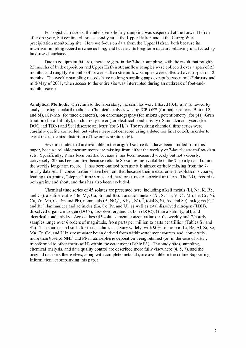
For logistical reasons, the intensive 7-hourly sampling was suspended at the Lower Hafren after one year, but continued for a second year at the Upper Hafren and at the Carreg Wen precipitation monitoring site. Here we focus on data from the Upper Hafren, both because its intensive sampling record is twice as long, and because its long-term data are relatively unaffected by land-use disturbance.

Due to equipment failures, there are gaps in the 7-hour sampling, with the result that roughly 22 months of bulk deposition and Upper Hafren streamflow samples were collected over a span of 23 months, and roughly 9 months of Lower Hafren streamflow samples were collected over a span of 12 months. The weekly sampling records have no long sampling gaps except between mid-February and mid-May of 2001, when access to the entire site was interrupted during an outbreak of foot-and-mouth disease.

Analytical Methods. On return to the laboratory, the samples were filtered (0.45 µm) followed by analysis using standard methods. Chemical analysis was by ICP-OES (for major cations, B, total S, and Si), ICP-MS (for trace elements), ion chromatography (for anions), potentiometry (for pH), Gran titration (for alkalinity), conductivity meter (for electrical conductivity), Shimadzu analysers (for DOC and TDN) and Seal discrete analyser (for NH4

+). The resulting chemical time series were carefully quality controlled, but values were not censored using a detection limit cutoff, in order to avoid the associated distortion of low concentrations (6).

Several solutes that are available in the original source data have been omitted from this paper, because reliable measurements are missing from either the weekly or 7-hourly streamflow data sets. Specifically, Y has been omitted because it has been measured weekly but not 7-hourly; conversely, Sb has been omitted because reliable Sb values are available in the 7-hourly data but not the weekly long-term record. I- has been omitted because it is almost entirely missing from the 7-hourly data set. F- concentrations have been omitted because their measurement resolution is coarse, leading to a grainy, "stepped" time series and therefore a risk of spectral artifacts. The NO2

- record is both grainy and short, and thus has also been excluded.

Chemical time series of 45 solutes are presented here, including alkali metals (Li, Na, K, Rb, and Cs), alkaline earths (Be, Mg, Ca, Sr, and Ba), transition metals (Al, Sc, Ti, V, Cr, Mn, Fe, Co, Ni, Cu, Zn, Mo, Cd, Sn and Pb), nonmetals (B, NO3

- , NH4+, SO4

-2, total S, Si, As, and Se), halogens (Cl- and Br-), lanthanides and actinides (La, Ce, Pr, and U), as well as total dissolved nitrogen (TDN), dissolved organic nitrogen (DON), dissolved organic carbon (DOC), Gran alkalinity, pH, and electrical conductivity. Across these 45 solutes, mean concentrations in the weekly and 7-hourly samples range over 6 orders of magnitude, from parts per million to parts per trillion (Tables S1 and S2). The sources and sinks for these solutes also vary widely, with 90% or more of Li, Be, Al, Si, Sc, Mn, Fe, Co, and U in streamwater being derived from within-catchment sources and, conversely, more than 90% of NH4

+ and Pb in atmospheric deposition being retained (or, in the case of NH4+,

transformed to other forms of N) within the catchment (Table S3). The study sites, sampling, chemical analysis, and data quality control are described more fully elsewhere (4, 5, 7), and the original data sets themselves, along with complete metadata, are available in the online Supporting Information accompanying this paper.

3

Fig. S2 (page 1 of 2). Water quality time series in Upper Hafren streamflow, Plynlimon, Wales, at 7-hour intervals for one year (left panels) and weekly intervals for 21 years (right panels). Shading in right-hand panels shows 2008, the year covered by left-hand panels.

4

Fig. S2 (page 2 of 2). Water quality time series in Upper Hafren streamflow, Plynlimon, Wales, at 7-hour intervals for one year (left panels) and weekly intervals for 21 years (right panels). Shading in right-hand panels shows 2008, the year covered by left-hand panels (except Cu and Sn, for which 2007 data are shown).

5

Table S1. Volume-weighted mean concentrations (± standard deviations) in 7-hourly samples of precipitation and Upper and Lower Hafren streamflow, Plynlimon, Wales.

Analyte Precipitation Upper Hafren Lower Hafren mean±s.d. mean±s.d. mean±s.d. Water flux mm/hr 0.34±0.77 0.32±0.39 0.25±0.38 Conductivity μS/cm 27.7±45.1 28.4±4.7 41.8±5.7 pH 4.71±0.65 5.09±0.47 4.70±0.39 Gran alkalinity μEq/l -27.1±39.5 -6.4±26.2 -22.0±24.9 Nutrients and anions, in order of increasing atomic number DOC mg/l 0.72±1.45 3.35±2.09 3.38±1.55 NO3

- mg(N)/l 0.14±0.26 0.14±0.07 0.18±0.06 NH4

+ mg(N)/l 0.177±0.183 0.028±0.039 0.026±0.019 TDN mg/l 0.335±0.537 0.279±0.093 0.305±0.068 DON mg/l -0.018±0.029 0.101±0.081 0.075±0.045 SO4

-2 mg(SO4)/l 1.21±1.36 1.92±0.30 3.01±0.40 Cl- mg/l 5.69±11.70 5.29±1.09 7.19±1.36 Br- μg/l 18.1±45.3 8.7±3.1 11.8±3.5 Metals and trace elements, in order of increasing atomic number Li μg/l 0.04±0.11 1.49±0.32 1.90±0.29 Be μg/l -0.003±0.004 0.018±0.009 0.042±0.017 B μg/l 2.49±3.14 3.39±0.52 4.10±0.40 Na mg/l 2.58±6.23 3.13±0.50 3.97±0.50 Mg mg/l 0.31±0.74 0.51±0.11 0.66±0.12 Al μg/l 2.9±10.1 121.6±63.2 197.8±81.3 Si mg/l 0.02±0.02 1.20±0.45 1.25±0.37 S mg/l 0.39±0.57 0.64±0.09 0.99±0.13 K mg/l 0.11±0.22 0.13±0.08 0.14±0.04 Ca mg/l 0.29±0.62 0.41±0.12 0.62±0.16 Sc μg/l n/a 0.25±0.17 0.25±0.13 Ti μg/l 0.02±0.10 0.32±0.11 0.27±0.10 V μg/l 0.18±0.24 0.09±0.04 0.11±0.04 Cr μg/l 1.01±8.89 0.14±0.08 0.24±0.08 Mn μg/l 0.6±2.1 16.6±3.2 29.5±7.4 Fe μg/l 3.1±10.7 123.2±78.2 116.3±59.7 Co μg/l 0.01±0.03 0.68±0.15 1.35±0.39 Ni μg/l 0.12±0.20 0.69±0.15 1.31±0.27 Cu μg/l n/a 5.9±7.1 1.7±0.7 Zn μg/l 6.6±9.1 11.0±5.7 12.0±3.7 As μg/l 0.075±0.087 0.228±0.067 0.247±0.062 Se μg/l 0.110±0.143 0.077±0.043 0.092±0.035 Rb μg/l 0.042±0.095 0.222±0.125 0.260±0.070 Sr μg/l 2.32±4.43 3.33±0.74 3.97±0.78 Mo μg/l 0.196±0.758 0.019±0.022 0.014±0.018 Cd μg/l n/a 0.026±0.011 0.044±0.014 Sn μg/l 0.035±0.399 0.042±0.031 0.056±0.025 Cs μg/l -0.002±0.004 0.016±0.005 0.020±0.006 Ba μg/l 6.73±11.50 1.67±0.45 2.34±0.49 La μg/l 0.017±0.094 0.017±0.008 0.028±0.010 Ce μg/l 0.018±0.121 0.049±0.025 0.083±0.033 Pr μg/l 0.003±0.015 0.008±0.004 0.015±0.006 Pb μg/l n/a 0.29±0.25 0.55±0.38 U μg/l -0.0031±0.0033 0.0024±0.0027 0.0049±0.0041 Analytes marked "n/a" were not measured in precipitation or yielded suspect values, and were therefore excluded from further analysis. Lower Hafren means cover only the first year of the two-year sampling program, and thus cannot be directly compared to means from Upper Hafren or precipitation. Mean and standard deviation of pH were calculated from H+. Analytes presented as ions are analyzed as ions; all others are total concentrations.

6

Table S2. Volume-weighted mean concentrations (± standard deviations) in long-term weekly sampling of precipitation and Upper and Lower Hafren streamflow, Plynlimon, Wales.

Analyte Precipitation Upper Hafren Lower Hafren mean±s.d. mean±s.d. mean±s.d. Water flux mm/hr 0.29±0.29 0.28±0.43 0.26±0.44 Conductivity μS/cm 24.7±18.9 32.7±8.0 43.3±9.8 pH 4.92±0.61 4.95±0.39 4.73±0.30 Gran alkalinity μEq/l -10.9±19.0 -3.9±19.5 -16.3±18.9 Nutrients and anions, in order of increasing atomic number DOC mg/l 0.53±0.45 2.48±1.72 2.69±1.81 NO3

- mg(N)/l 0.17±0.22 0.20±0.12 0.30±0.15 NH4

+ mg(N)/l 0.201±0.267 0.015±0.014 0.015±0.026 TDN mg/l 0.32±0.32 0.34±0.10 0.45±0.15 DON mg/l 0.041±0.074 0.158±0.092 0.188±0.102 SO4

-2 mg(SO4)/l 1.02±0.53 1.81±0.34 2.80±0.52 Cl- mg/l 4.33±4.48 5.70±1.62 7.10±1.94 Br- μg/l 13.8±13.9 10.8±4.9 15.1±5.2 Metals and trace elements, in order of increasing atomic number Li μg/l 0.08±0.12 1.64±0.41 2.00±0.45 Be μg/l 0.000±0.004 0.019±0.010 0.065±0.032 B μg/l 3.9±6.9 4.2±1.4 5.1±1.5 Na mg/l 2.27±2.38 3.30±0.64 3.97±0.72 Mg mg/l 0.28±0.30 0.57±0.14 0.71±0.16 Al μg/l 17.2±39.6 156.6±83.1 291.7±133.2 Si mg/l 0.09±0.34 1.19±0.49 1.24±0.43 S mg/l 0.47±0.34 0.76±0.17 1.27±0.31 K mg/l 0.11±0.10 0.18±0.08 0.20±0.09 Ca mg/l 0.20±0.28 0.45±0.13 0.71±0.19 Sc μg/l 0.00±0.07 0.37±0.21 0.40±0.19 Ti μg/l 0.21±0.40 0.51±0.31 0.53±0.33 V μg/l 0.22±0.14 0.14±0.09 0.17±0.08 Cr μg/l 1.04±2.47 0.29±0.28 1.46±3.29 Mn μg/l 1.1±2.0 19.5±4.8 38.2±12.2 Fe μg/l 7.6±15.8 126.0±66.4 123.4±59.8 Co μg/l 0.04±0.17 0.79±0.23 1.74±0.62 Ni μg/l 0.38±0.78 1.06±0.51 1.89±0.65 Cu μg/l 3.1±7.3 3.3±11.1 2.9±5.3 Zn μg/l 12.0±15.8 19.2±14.4 20.3±12.2 As μg/l 0.08±0.06 0.28±0.11 0.31±0.09 Se μg/l 0.14±0.09 0.13±0.05 0.15±0.06 Rb μg/l 0.10±0.11 0.29±0.15 0.36±0.17 Sr μg/l 1.92±1.73 3.86±0.94 4.68±1.14 Mo μg/l 0.037±0.165 0.023±0.016 0.026±0.025 Cd μg/l 0.045±0.152 0.035±0.022 0.058±0.036 Sn μg/l 0.104±0.106 0.093±0.118 0.093±0.121 Cs μg/l 0.005±0.009 0.020±0.010 0.031±0.011 Ba μg/l 5.0±13.5 2.7±0.9 4.4±2.5 La μg/l 0.031±0.101 0.021±0.014 0.034±0.023 Ce μg/l 0.017±0.085 0.053±0.028 0.095±0.038 Pr μg/l 0.007±0.018 0.010±0.006 0.015±0.008 Pb μg/l 10.80±42.27 0.43±0.48 0.82±0.79 U μg/l 0.0001±0.0032 0.0046±0.0039 0.0090±0.0045 Precipitation and Lower Hafren measurements span 10 May 1983 to 11 October 2011. Upper Hafren measurements span 17 July 1990 to 11 October 2011. Mean and standard deviation of pH were calculated from H+. Analytes presented as ions are analyzed as ions; all others are total concentrations.

7

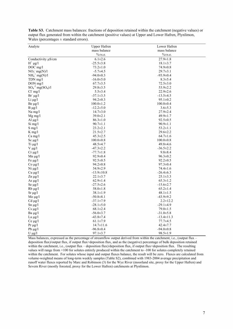
Table S3. Catchment mass balances: fractions of deposition retained within the catchment (negative values) or output flux generated from within the catchment (positive values) at Upper and Lower Hafren, Plynlimon, Wales (percentages ± standard errors).

Analyte Upper Hafren Lower Hafren mass balance mass balance %±s.e. %±s.e. Conductivity μS/cm 6.1±2.6 27.9±1.8 H+ μg/l -25.5±3.8 18.1±3.7 DOC mg/l 73.2±1.0 74.9±0.8 NO3

- mg(N)/l -5.7±4.5 29.7±3.1 NH4

+ mg(N)/l -94.0±0.3 -93.9±0.4 TDN mg/l -16.0±5.0 8.3±5.4 DON mg/l 67.7±3.5 72.5±3.0 SO4

-2 mg(SO4)/l 29.8±3.5 53.9±2.2 Cl- mg/l 5.5±3.4 22.9±2.6 Br- μg/l -37.1±3.5 -13.5±4.5 Li μg/l 94.2±0.3 95.1±0.2 Be μg/l 100.0±1.2 100.0±0.4 B μg/l -12.2±5.0 3.6±5.3 Na mg/l 14.7±3.0 27.9±2.4 Mg mg/l 39.0±2.1 49.9±1.7 Al μg/l 86.3±1.0 92.5±0.5 Si mg/l 90.7±1.1 90.9±1.1 S mg/l 23.2±2.1 53.2±1.1 K mg/l 21.5±2.7 29.6±2.2 Ca mg/l 45.3±2.5 64.7±1.6 Sc μg/l 100.0±0.8 100.0±0.8 Ti μg/l 48.5±4.7 49.8±4.6 V μg/l -47.3±2.2 -36.5±2.2 Cr μg/l -77.7±1.8 9.8±8.4 Mn μg/l 92.9±0.4 96.3±0.2 Fe μg/l 92.5±0.5 92.2±0.5 Co μg/l 94.2±0.8 97.3±0.4 Ni μg/l 54.9±2.9 74.4±1.6 Cu μg/l -13.9±10.8 -26.4±6.3 Zn μg/l 22.1±3.7 25.1±3.3 As μg/l 62.9±1.4 65.3±1.2 Se μg/l -27.5±2.6 -15.6±2.7 Rb μg/l 58.0±1.8 65.2±1.4 Sr μg/l 38.1±1.9 48.1±1.5 Mo μg/l -50.8±8.1 -43.9±9.2 Cd μg/l -37.1±7.9 2.2±12.2 Sn μg/l -28.1±5.0 -29.1±4.9 Cs μg/l 68.1±2.4 79.0±1.5 Ba μg/l -56.0±3.7 -31.0±5.8 La μg/l -43.8±7.4 -13.4±11.3 Ce μg/l 61.1±7.9 77.7±4.5 Pr μg/l 14.7±11.6 42.4±7.7 Pb μg/l -96.8±0.4 -94.0±0.8 U μg/l 97.1±3.7 98.5±1.9 Mass balances, expressed as the percentage of streamflow output derived from within the catchment, i.e., (output flux – deposition flux)/output flux, if output flux>deposition flux, and as the (negative) percentage of bulk deposition retained within the catchment, i.e., (output flux – deposition flux)/deposition flux, if output flux<deposition flux. The resulting values will range from +100 for solutes entirely produced within the catchment to -100 for solutes completely retained within the catchment. For solutes whose input and output fluxes balance, the result will be zero. Fluxes are calculated from volume-weighted means of long-term weekly samples (Table S2), combined with 1983-2004 average precipitation and runoff water fluxes reported by Marc and Robinson (3) for the Wye River (moorland site, proxy for the Upper Hafren) and Severn River (mostly forested, proxy for the Lower Hafren) catchments at Plynlimon.

8

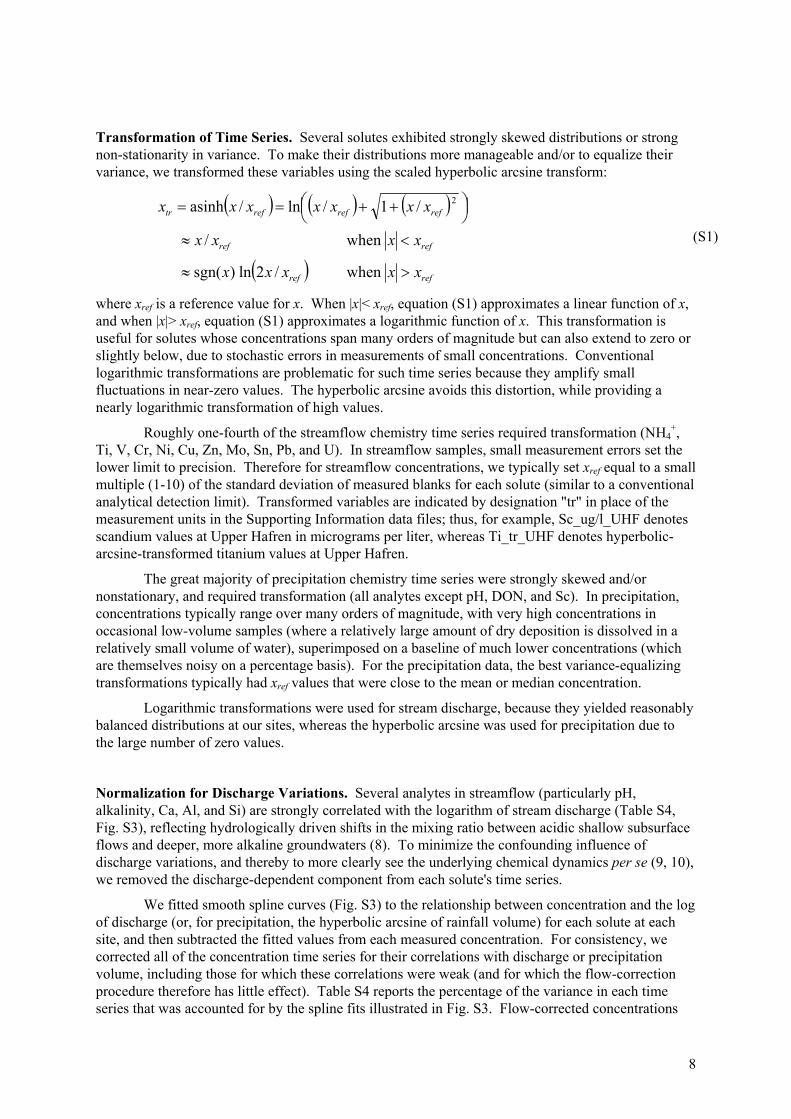
Transformation of Time Series. Several solutes exhibited strongly skewed distributions or strong non-stationarity in variance. To make their distributions more manageable and/or to equalize their variance, we transformed these variables using the scaled hyperbolic arcsine transform:

refref

refref

refrefreftr

xxxxx

xxxx

xxxxxxx

when/2ln)sgn(

when/

/1/ln/asinh 2

(S1)

where xref is a reference value for x. When |x|< xref, equation (S1) approximates a linear function of x, and when |x|> xref, equation (S1) approximates a logarithmic function of x. This transformation is useful for solutes whose concentrations span many orders of magnitude but can also extend to zero or slightly below, due to stochastic errors in measurements of small concentrations. Conventional logarithmic transformations are problematic for such time series because they amplify small fluctuations in near-zero values. The hyperbolic arcsine avoids this distortion, while providing a nearly logarithmic transformation of high values.

Roughly one-fourth of the streamflow chemistry time series required transformation (NH4+,

Ti, V, Cr, Ni, Cu, Zn, Mo, Sn, Pb, and U). In streamflow samples, small measurement errors set the lower limit to precision. Therefore for streamflow concentrations, we typically set xref equal to a small multiple (1-10) of the standard deviation of measured blanks for each solute (similar to a conventional analytical detection limit). Transformed variables are indicated by designation "tr" in place of the measurement units in the Supporting Information data files; thus, for example, Sc_ug/l_UHF denotes scandium values at Upper Hafren in micrograms per liter, whereas Ti_tr_UHF denotes hyperbolic-arcsine-transformed titanium values at Upper Hafren.

The great majority of precipitation chemistry time series were strongly skewed and/or nonstationary, and required transformation (all analytes except pH, DON, and Sc). In precipitation, concentrations typically range over many orders of magnitude, with very high concentrations in occasional low-volume samples (where a relatively large amount of dry deposition is dissolved in a relatively small volume of water), superimposed on a baseline of much lower concentrations (which are themselves noisy on a percentage basis). For the precipitation data, the best variance-equalizing transformations typically had xref values that were close to the mean or median concentration.

Logarithmic transformations were used for stream discharge, because they yielded reasonably balanced distributions at our sites, whereas the hyperbolic arcsine was used for precipitation due to the large number of zero values.

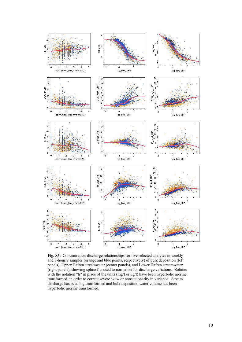
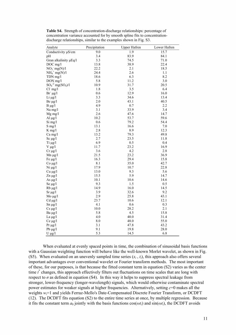
Normalization for Discharge Variations. Several analytes in streamflow (particularly pH, alkalinity, Ca, Al, and Si) are strongly correlated with the logarithm of stream discharge (Table S4, Fig. S3), reflecting hydrologically driven shifts in the mixing ratio between acidic shallow subsurface flows and deeper, more alkaline groundwaters (8). To minimize the confounding influence of discharge variations, and thereby to more clearly see the underlying chemical dynamics per se (9, 10), we removed the discharge-dependent component from each solute's time series.

We fitted smooth spline curves (Fig. S3) to the relationship between concentration and the log of discharge (or, for precipitation, the hyperbolic arcsine of rainfall volume) for each solute at each site, and then subtracted the fitted values from each measured concentration. For consistency, we corrected all of the concentration time series for their correlations with discharge or precipitation volume, including those for which these correlations were weak (and for which the flow-correction procedure therefore has little effect). Table S4 reports the percentage of the variance in each time series that was accounted for by the spline fits illustrated in Fig. S3. Flow-corrected concentrations

9

are indicated by the designation "fc" in the Supporting Information data files; thus, for example, Ca_mg/l_UHF denotes calcium values at Upper Hafren in milligrams per liter, whereas fc_Ca_mg/l_UHF denotes flow-corrected calcium values at Upper Hafren.

Removing the confounding influence of discharge variations affects the resulting power spectra to varying degrees (Fig. S4), depending on the strength of the concentration-discharge relationship. For example, 84 percent of the variance in pH is explained by variations in the logarithm of discharge (Fig. S3, Table S4), so the pH time series (Fig. S2) and their un-corrected power spectra (Fig. S4) strongly resemble the time series and power spectrum of log(Q). When the discharge-dependent component of the pH time series is removed, however, the underlying chemical dynamics are revealed to have a clear 1/f spectral signature (Fig. S4). In the five cases noted above (pH, alkalinity, Ca, Al, and Si) the 1/f spectral signature of the chemical dynamics is substantially overprinted by the power spectrum of log(Q), and in all five cases, the flow-corrected concentrations remove this overprinting. For the 40 other solutes, the flow-corrected and un-corrected concentrations both have substantially similar 1/f power spectra.

The solutes shown in Fig. S4 have been selected to show a range of discharge-dependence. The discharge-dependence of pH (R2=0.84) is the strongest of any of the solutes. More than five-sixths of the solutes have weaker discharge-dependence than Mg (R2=0.48), which is shown second in Fig. S4. Fully three-fourths of the solutes have weaker discharge-dependence than Co (R2=0.35), and Mn (R2=0.23) lies near the mean and median discharge-dependence (R2=0.25 and 0.20, respectively) of the 45 solutes. The figures quoted here are for solutes in Upper Hafren streamflow; solutes in Lower Hafren exhibit weaker discharge-dependence overall (Table S4).

Estimation of Power Spectra. Data gaps occurred intermittently due to autosampler failure or analytical problems, and also whenever rainfall yielded insufficient volume for chemical analysis. Such gapped time series require special Fourier analysis techniques, particularly for colored noise spectra, because spectral leakage from low frequencies with high power can contaminate the higher frequencies in the spectrum where the true signal is weaker. We used an adaptation of Foster's weighted wavelet transform (11) to suppress this leakage in estimating the spectrum.

Foster's weighted wavelet transform is formally equivalent to a weighted least-squares multiple regression fit of a time series (xi , ti) to a constant and two basis functions, namely the sine and cosine waves at a specified frequency

iii tataax sincos 210 (S2)

where a0, a1, and a2 are where best-fit regression coefficients, and where each data point is weighted by a Gaussian function of the difference between its time ti and the center time of the wavelet, t*:

2*2exp ttcw ii (S3)

In equation (S3), c is a parameter that controls how fast the Gaussian weight falls off with distance from the center. In terms of the equivalent standard deviation, the width of the Gaussian bell curve is

cc 2

112 (S4)

where λ is the period of oscillation corresponding to the angular frequency ω. As with any windowed Fourier transform, the wider the window (i.e., the smaller the value of c), the sharper the frequency resolution in the resulting power spectrum. We set c=0.001 in order to clearly resolve seasonal and diurnal cycles in the concentration time series.

10

Fig. S3. Concentration-discharge relationships for five selected analytes in weekly and 7-hourly samples (orange and blue points, respectively) of bulk deposition (left panels), Upper Hafren streamwater (center panels), and Lower Hafren streamwater (right panels), showing spline fits used to normalize for discharge variations. Solutes with the notation "tr" in place of the units (mg/l or μg/l) have been hyperbolic arcsine transformed, in order to correct severe skew or nonstationarity in variance. Stream discharge has been log transformed and bulk deposition water volume has been hyperbolic arcsine transformed.

11

Table S4. Strength of concentration-discharge relationships: percentage of concentration variance accounted for by smooth spline fits to concentration-discharge relationships, similar to the examples shown in Fig. S3.

Analyte Precipitation Upper Hafren Lower Hafren Conductivity μS/cm 9.0 1.9 15.7 pH 3.4 83.9 84.1 Gran alkalinity μEq/l 3.3 74.5 71.0 DOC mg/l 13.8 38.9 22.4 NO3

- mg(N)/l 22.2 2.1 18.5 NH4

+ mg(N)/l 24.4 2.6 1.1 TDN mg/l 18.6 6.3 8.2 DON mg/l 5.8 11.2 3.0 SO4

-2 mg(SO4)/l 10.9 31.7 20.5 Cl- mg/l 1.8 3.5 6.4 Br- μg/l 0.6 12.9 16.0 Li μg/l 3.3 34.6 13.4 Be μg/l 2.0 43.1 40.5 B μg/l 4.9 0.7 2.2 Na mg/l 3.1 33.9 3.4 Mg mg/l 2.6 47.6 14.7 Al μg/l 10.2 53.7 59.6 Si mg/l 0.6 79.2 54.4 S mg/l 13.1 16.6 7.0 K mg/l 2.8 8.9 12.3 Ca mg/l 13.2 79.3 49.8 Sc μg/l 2.7 23.5 11.8 Ti μg/l 6.9 0.5 0.4 V μg/l 11.7 23.2 16.9 Cr μg/l 3.6 4.2 2.8 Mn μg/l 21.5 23.2 36.9 Fe μg/l 16.3 29.4 15.8 Co μg/l 8.1 35.0 42.7 Ni μg/l 17.9 10.7 22.8 Cu μg/l 13.0 9.3 5.6 Zn μg/l 15.5 5.9 14.7 As μg/l 10.1 10.6 14.6 Se μg/l 9.3 1.5 0.5 Rb μg/l 14.9 16.0 14.5 Sr μg/l 3.9 32.6 9.2 Mo μg/l 2.9 25.8 43.1 Cd μg/l 23.7 10.6 12.1 Sn μg/l 4.1 0.6 0.3 Cs μg/l 10.0 28.2 2.1 Ba μg/l 5.8 4.5 15.8 La μg/l 4.0 40.0 31.4 Ce μg/l 8.0 48.0 55.0 Pr μg/l 3.1 47.8 43.2 Pb μg/l 9.1 19.8 28.0 U μg/l 5.3 14.5 6.8

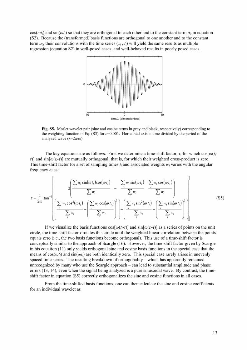
When evaluated at evenly spaced points in time, the combination of sinusoidal basis functions with a Gaussian weighting function will behave like the well-known Morlet wavelet, as shown in Fig. (S5). When evaluated on an unevenly sampled time series (xi , ti), this approach also offers several important advantages over conventional wavelet or Fourier transform methods. The most important of these, for our purposes, is that because the fitted constant term in equation (S2) varies as the center time t* changes, this approach effectively filters out fluctuations on time scales that are long with respect to σ as defined in equation (S4). In this way it helps to suppress spectral leakage from stronger, lower-frequency (longer-wavelength) signals, which would otherwise contaminate spectral power estimates for weaker signals at higher frequencies. Alternatively, setting c=0 makes all the weights wi=1 and yields Ferraz-Mello's Date-Compensated Discrete Fourier Transform, or DCDFT (12). The DCDFT fits equation (S2) to the entire time series at once, by multiple regression. Because it fits the constant term a0 jointly with the basis functions cos(ωti) and sin(ωti), the DCDFT avoids

12

distortions that can arise when this constant term is omitted (13, 14), as is the case, for example, in the more widely known Lomb-Scargle Fourier Transform, or LSFT (15, 16). However, neither the DCDFT nor the LSFT suppresses spectral leakage from lower frequencies to higher frequencies, which is the great advantage of Foster's wavelet-based approach.

100

102

104

106

108

1010

1012

1014

1016

0.01 0.1 1 10 100 1000

Sp

ect

ral p

owe

r (a

rbitr

ary

log

sca

le)

Frequency (1/yr, log scale)

(R2=0.84)

Mg

Co

Mn

Ni

log(Q)

pH

(R2=0.48)

(R2=0.35)

(R2=0.23)

(R2=0.11)

Fig. S4. Sample power spectra, with and without flow-correction (colored and gray symbols, respectively), of solute concentrations in Upper Hafren streamflow. The spectrum of the logarithm of discharge (dark gray and black symbols) is non-fractal, scaling as white noise at low frequencies and steepening to 1/f 2 at frequencies of roughly 80-600/year (short gray lines show slopes of 0 and 2 for comparison). The spectra of the un-corrected solute concentrations (light gray symbols) reflect the non-fractal signature of discharge to varying degrees, depending on the strength of the correlation between concentration and discharge. The spectra of the flow-corrected concentrations (colored symbols), by contrast, exhibit fractal 1/f scaling (long gray lines show slopes of 1 for comparison), regardless of the degree of discharge-dependence in the un-corrected time series. Spectra for individual analytes have been shifted by arbitrary factors to allow them to be visualized together, but pairs of flow-corrected and un-corrected spectra for individual analytes are plotted on consistent axes (thus differences between them reflect real differences in spectral power). Quoted R2 values from Table S4 express the fraction of concentration variance explained by spline fits to the log of discharge (see Fig. S3).

The drawback to Foster's approach, however, is that when equation (S2) is estimated by multiple regression on unevenly sampled data, the values of the fitted coefficients can become unrealistically large, and thus the spectral power estimates can become unreliable, whenever the variance-covariance matrix becomes singular or nearly so. This results in spurious spikes in the power spectrum. These spurious spikes become more frequent as the weighting window becomes narrower, the sampling times become more uneven, and the mesh of sampled frequencies ω becomes denser.

We avoid this problem entirely by re-casting the weighted regression in equations (S2-S3) as a convolution instead. Specifically, we convolve the time series xi (ti) with the two basis functions cos(ωti) and sin(ωti), with each point weighted by wi as defined in (S3), after first transforming

13

cos(ωti) and sin(ωti) so that they are orthogonal to each other and to the constant term a0 in equation (S2). Because the (transformed) basis functions are orthogonal to one another and to the constant term a0, their convolutions with the time series (xi , ti) will yield the same results as multiple regression (equation S2) in well-posed cases, and well-behaved results in poorly posed cases.

0

-10 0 10time/ (dimensionless)

Fig. S5. Morlet wavelet pair (sine and cosine terms in gray and black, respectively) corresponding to the weighting function in Eq. (S3) for c=0.001. Horizontal axis is time divided by the period of the analyzed wave (λ=2π/ω).

The key equations are as follows. First we determine a time-shift factor, τ, for which cos[ω(ti-τ)] and sin[ω(ti-τ)] are mutually orthogonal; that is, for which their weighted cross-product is zero. This time-shift factor for a set of sampling times ti and associated weights wi varies with the angular frequency ω as:

2222

1

sinsincoscos

cossincossin

2

tan2

1

ii

iii

ii

iii

ii

iii

ii

iii

ii

iii

ii

iii

ii

iiii

w

tw

w

tw

w

tw

w

tw

w

tw

w

tw

w

ttw

(S5)

If we visualize the basis functions cos[ω(ti-τ)] and sin[ω(ti-τ)] as a series of points on the unit circle, the time-shift factor τ rotates this circle until the weighted linear correlation between the points equals zero (i.e., the two basis functions become orthogonal). This use of a time-shift factor is conceptually similar to the approach of Scargle (16). However, the time-shift factor given by Scargle in his equation (11) only yields orthogonal sine and cosine basis functions in the special case that the means of cos(ωti) and sin(ωti) are both identically zero. This special case rarely arises in unevenly spaced time series. The resulting breakdown of orthogonality – which has apparently remained unrecognized by many who use the Scargle approach – can lead to substantial amplitude and phase errors (13, 14), even when the signal being analyzed is a pure sinusoidal wave. By contrast, the time-shift factor in equation (S5) correctly orthogonalizes the sine and cosine functions in all cases.

From the time-shifted basis functions, one can then calculate the sine and cosine coefficients for an individual wavelet as

14

ii

iii

ii

iii

ii

iiii

ii

iii

ii

iii

ii

iiii

w

tw

w

xw

w

txw

w

tw

w

xw

w

txwa

sinsinsin2

coscoscos21

(S6)

and

ii

iii

ii

iii

ii

iiii

ii

iii

ii

iii

ii

iiii

w

tw

w

xw

w

txw

w

tw

w

xw

w

txwa

sinsincos2

coscossin22

(S7)

The formulation of equations (S6) and (S7) guarantees orthogonality between the weighted sine and cosine functions and the constant term a0, by convolving the weighted time series with the weighted basis functions after subtracting each of their means. This approach thus achieves the same benefits as the local fitting of a0 in Foster's approach, without the associated instabilities in poorly posed cases. The leading terms cos(ωτ) and sin(ωτ) in equations (S6) and (S7) serve to undo the time shift τ, to yield the correct Fourier coefficients a1 and a2 for the original time base. The spectral power estimate from each individual wavelet is then calculated as:

n

nttaaS eff

X minmax22

215.0 (S8)

where tmax-tmin expresses the time interval covered by the n sampled points, and neff is the "effective" number of points, a correction for the unevenness of the weighting among the points, calculated following Foster (11) as:

ii

ii

effw

w

n 2

2

(S9)

We estimate spectral power for wavelets centered at evenly spaced points along the length of the time series using equations (S5-S9). These individual spectral power estimates are then pooled by taking their mean, weighted by the degrees of freedom associated with each estimate, which equals neff -3. For neff<3, the degrees of freedom, and thus the associated weight of the spectral power estimate, are assigned a value of zero.

Further computational details can be found in the computer code spectral_analysis.c, which is available, along with all necessary input files and selected output files, from the corresponding author.

15

Smoothing and Alias-filtering of Power Spectra. Conventional Fourier transform methods typically yield noisy spectral power estimates for individual frequencies. The resulting wedge-shaped power spectrum, which is narrow at low frequencies and becomes ever-wider at high frequencies, can be problematic in at least two respects. First, it can be difficult to see the shape of the broad-band spectrum within the wedge of widely varying spectral estimates at high frequencies. And second, this wedge can appear steeper than the average broad-band power spectrum is, because the logarithmic axis amplifies downward fluctuations more than upward fluctuations (for an illustrative example, see Fig. 3 of ref. 17).

The weighted wavelet approach outlined above analyzes the time series in overlapping windows, which scale with the wavelength of the analyzed wave. This windowing has the effect that spectral power estimates at any frequency will represent the average spectral power over a range of neighboring frequencies. The range over which frequencies are averaged is constant in logarithmic terms, meaning that at higher frequencies, where spectral estimates are more uncertain, a greater number of them are averaged together and thus the uncertainty in the broad-band average becomes roughly constant on a logarithmic scale. This is desirable for our purposes, because we are primarily interested in the spectral slope of the broad-band noise. (Our spectral analysis code also provides for analogous smoothing of Fourier transforms that are performed without local windowing. The power spectrum is smoothed using a Gaussian window with a width of 0.05 log units in frequency, which yields a similar degree of smoothing as the wavelet-based approach outlined above, with c=0.001.)

Regardless of the spectral analysis method one uses, spectral estimates are generally contaminated by aliasing of spectral power from above the Nyquist frequency, because the gapped sampling has a regular (weekly or seven-hourly) time base. This spectral aliasing leads to an artificial flattening of the spectrum at high frequencies and can be particularly severe in 1/f noises (17), because these typically contain significant power above the Nyquist frequency. We used Kirchner's filtering method (17) to correct for this spectral aliasing. The weekly time series has a lower Nyquist frequency than the 7-hourly time series, and this will be reflected in a greater degree of spectral aliasing. Conversely, because the 7-hourly time series is less affected by aliasing, it can help in inferring an accurate spectral model for the aliasing filter, which can then be applied to spectra derived from both the 7-hourly and weekly data.

Therefore we have adapted Kirchner's alias-filtering method so that it fits a single spectral model jointly to the smoothed spectra of both the 7-hourly and weekly data. Our approach allows a constant offset between the 7-hourly and weekly spectra, because some solutes exhibit different variance during the two years that were intensively sampled than they do on average over the decades of our long-term time series. The only user-determined parameter in our alias-filtering method is the corner frequency fc, above which the spectrum is assumed to steepen significantly. We set fc at 1460/year, corresponding to a wavelength of 6 hours, based on high-frequency measurements of pH and conductivity at Plynlimon (18, 19) showing that at time scales shorter than about 3 hours, both concentrations and stream discharge become relatively smooth functions of time. The choice of fc has only a weak effect on the measured spectral slopes. The alias-filtered spectra for all 45 solutes at both sampling sites are shown in Fig. S6.

Estimation of Spectral Slopes. To estimate the spectral slope (Fig. 3, Table S5), we fitted a single least-squares regression slope jointly to the alias-filtered weekly and 7-hourly spectra. As with the alias-filtering routine, we allowed a constant offset between the two spectra, to account for possible differences in overall variance between the two intensively sampled years and the decades of long-term data. The reported uncertainties in the slopes are corrected for the effects of the spectral smoothing on the correlations among the regression residuals. Further computational details can be found in the computer code alias_filter.c, which is available, along with all necessary input files and selected output files, from the corresponding author.

16

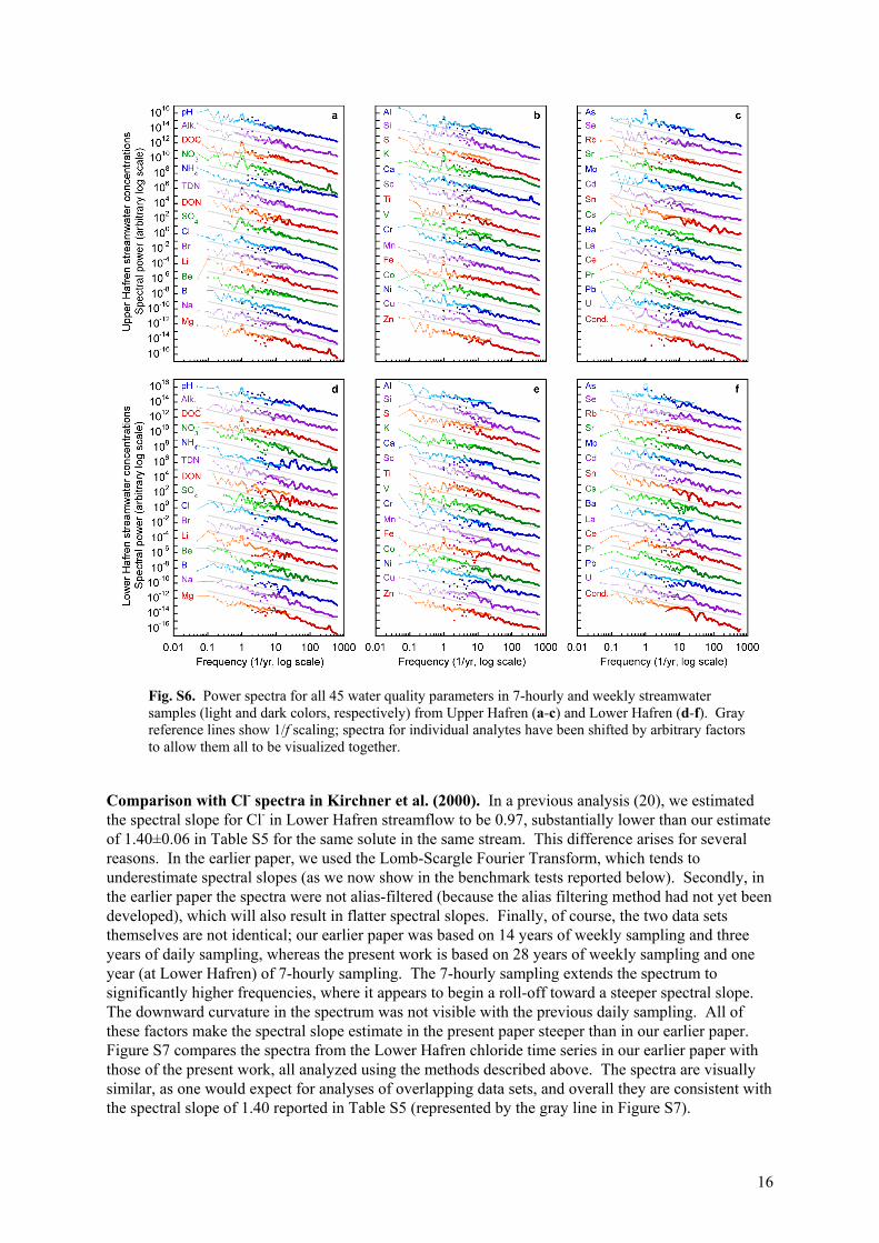
Fig. S6. Power spectra for all 45 water quality parameters in 7-hourly and weekly streamwater samples (light and dark colors, respectively) from Upper Hafren (a-c) and Lower Hafren (d-f). Gray reference lines show 1/f scaling; spectra for individual analytes have been shifted by arbitrary factors to allow them all to be visualized together.

Comparison with Cl- spectra in Kirchner et al. (2000). In a previous analysis (20), we estimated the spectral slope for Cl- in Lower Hafren streamflow to be 0.97, substantially lower than our estimate of 1.40±0.06 in Table S5 for the same solute in the same stream. This difference arises for several reasons. In the earlier paper, we used the Lomb-Scargle Fourier Transform, which tends to underestimate spectral slopes (as we now show in the benchmark tests reported below). Secondly, in the earlier paper the spectra were not alias-filtered (because the alias filtering method had not yet been developed), which will also result in flatter spectral slopes. Finally, of course, the two data sets themselves are not identical; our earlier paper was based on 14 years of weekly sampling and three years of daily sampling, whereas the present work is based on 28 years of weekly sampling and one year (at Lower Hafren) of 7-hourly sampling. The 7-hourly sampling extends the spectrum to significantly higher frequencies, where it appears to begin a roll-off toward a steeper spectral slope. The downward curvature in the spectrum was not visible with the previous daily sampling. All of these factors make the spectral slope estimate in the present paper steeper than in our earlier paper. Figure S7 compares the spectra from the Lower Hafren chloride time series in our earlier paper with those of the present work, all analyzed using the methods described above. The spectra are visually similar, as one would expect for analyses of overlapping data sets, and overall they are consistent with the spectral slope of 1.40 reported in Table S5 (represented by the gray line in Figure S7).

17

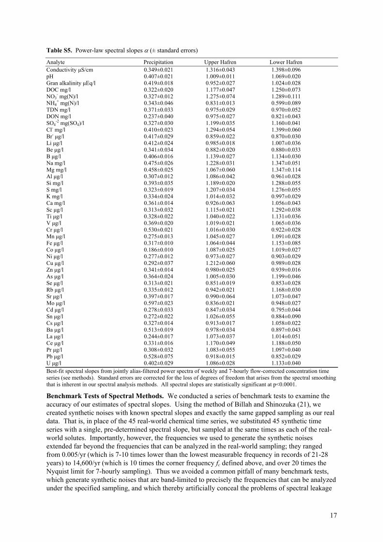
Table S5. Power-law spectral slopes (± standard errors)

Analyte Precipitation Upper Hafren Lower Hafren Conductivity μS/cm 0.349±0.021 1.316±0.043 1.398±0.096 pH 0.407±0.021 1.009±0.011 1.069±0.020 Gran alkalinity μEq/l 0.419±0.018 0.952±0.027 1.024±0.028 DOC mg/l 0.322±0.020 1.177±0.047 1.250±0.073 NO3

- mg(N)/l 0.327±0.012 1.275±0.074 1.289±0.111 NH4

+ mg(N)/l 0.343±0.046 0.831±0.013 0.599±0.089 TDN mg/l 0.371±0.033 0.975±0.029 0.970±0.052 DON mg/l 0.237±0.040 0.975±0.027 0.821±0.043 SO4

-2 mg(SO4)/l 0.327±0.030 1.199±0.035 1.160±0.041 Cl- mg/l 0.410±0.023 1.294±0.054 1.399±0.060 Br- μg/l 0.417±0.029 0.859±0.022 0.870±0.030 Li μg/l 0.412±0.024 0.985±0.018 1.007±0.036 Be μg/l 0.341±0.034 0.882±0.020 0.880±0.033 B μg/l 0.406±0.016 1.139±0.027 1.134±0.030 Na mg/l 0.475±0.026 1.228±0.031 1.347±0.051 Mg mg/l 0.458±0.025 1.067±0.060 1.347±0.114 Al μg/l 0.307±0.012 1.086±0.042 0.961±0.028 Si mg/l 0.393±0.035 1.189±0.020 1.288±0.055 S mg/l 0.323±0.019 1.207±0.034 1.276±0.055 K mg/l 0.334±0.024 1.014±0.032 0.997±0.029 Ca mg/l 0.361±0.014 0.926±0.063 1.056±0.043 Sc μg/l 0.313±0.032 1.115±0.021 1.292±0.038 Ti μg/l 0.328±0.022 1.040±0.022 1.131±0.036 V μg/l 0.369±0.020 1.019±0.021 1.065±0.036 Cr μg/l 0.530±0.021 1.016±0.030 0.922±0.028 Mn μg/l 0.275±0.013 1.045±0.027 1.091±0.028 Fe μg/l 0.317±0.010 1.064±0.044 1.153±0.085 Co μg/l 0.186±0.010 1.087±0.025 1.019±0.027 Ni μg/l 0.277±0.012 0.973±0.027 0.903±0.029 Cu μg/l 0.292±0.037 1.212±0.060 0.989±0.028 Zn μg/l 0.341±0.014 0.980±0.025 0.939±0.016 As μg/l 0.364±0.024 1.005±0.030 1.199±0.046 Se μg/l 0.313±0.021 0.851±0.019 0.853±0.028 Rb μg/l 0.335±0.012 0.942±0.021 1.168±0.030 Sr μg/l 0.397±0.017 0.990±0.064 1.073±0.047 Mo μg/l 0.597±0.023 0.836±0.021 0.948±0.027 Cd μg/l 0.278±0.033 0.847±0.034 0.795±0.044 Sn μg/l 0.272±0.022 1.026±0.055 0.884±0.090 Cs μg/l 0.327±0.014 0.913±0.017 1.058±0.022 Ba μg/l 0.513±0.019 0.978±0.034 0.897±0.043 La μg/l 0.244±0.017 1.073±0.037 1.014±0.051 Ce μg/l 0.331±0.016 1.170±0.049 1.188±0.050 Pr μg/l 0.308±0.032 1.083±0.055 1.097±0.040 Pb μg/l 0.528±0.075 0.918±0.015 0.852±0.029 U μg/l 0.402±0.029 1.086±0.028 1.133±0.040 Best-fit spectral slopes from jointly alias-filtered power spectra of weekly and 7-hourly flow-corrected concentration time series (see methods). Standard errors are corrected for the loss of degrees of freedom that arises from the spectral smoothing that is inherent in our spectral analysis methods. All spectral slopes are statistically significant at p<0.0001.

Benchmark Tests of Spectral Methods. We conducted a series of benchmark tests to examine the accuracy of our estimates of spectral slopes. Using the method of Billah and Shinozuka (21), we created synthetic noises with known spectral slopes and exactly the same gapped sampling as our real data. That is, in place of the 45 real-world chemical time series, we substituted 45 synthetic time series with a single, pre-determined spectral slope, but sampled at the same times as each of the real-world solutes. Importantly, however, the frequencies we used to generate the synthetic noises extended far beyond the frequencies that can be analyzed in the real-world sampling; they ranged from 0.005/yr (which is 7-10 times lower than the lowest measurable frequency in records of 21-28 years) to 14,600/yr (which is 10 times the corner frequency fc defined above, and over 20 times the Nyquist limit for 7-hourly sampling). Thus we avoided a common pitfall of many benchmark tests, which generate synthetic noises that are band-limited to precisely the frequencies that can be analyzed under the specified sampling, and which thereby artificially conceal the problems of spectral leakage

18

(from low frequencies) and spectral aliasing (from high frequencies) that afflict real-world spectral analyses. Further computational details can be found in the computer code benchmark_generator.c, which is available from the corresponding author.

10-5

10-4

10-3

10-2

10-1

100

101

0.01 0.1 1 10 100 1000

Sp

ect

ral p

ow

er

((m

g/L

)2-y

r)

Frequency (1/yr, log scale)

3 yr daily

1 yr 7-hourly

14 yr weekly

28 yr weekly

Fig. S7. Lower Hafren streamflow Cl- power spectra calculated in the present work (light and dark blue symbols representing weekly and 7-hourly sampling, respectively), compared to the same spectral methods applied to the data of ref. (20), with orange and red symbols representing weekly and daily sampling, respectively. Gray line indicates a spectral slope of 1.40 (see Table S5).

Fig. S8. Benchmark tests for spectral analysis of Upper Hafren water quality data. Each panel shows the distribution of spectral slopes estimated from synthetic benchmark time series with spectral power scaling as 1/f , with ranging from 0 to 2 in steps of 0.25 (gray lines). These benchmark time series were sampled at the same times and with the same gaps as the 45 water quality parameters in Upper Hafren streamflow. They were then analyzed by the same methods as those used for the real-world water quality data (our variant of Foster's Weighted Wavelet Transform, left column), and by the Date-Compensated Discrete Fourier Transform, or DCDFT (12, 22) (right column). Results from the Lomb-Scargle Fourier Transform, or LSFT (15, 16) are visually indistinguishable from those obtained with the DCDFT. All spectra were alias-filtered by the identical procedure used with the real-world data. Spectral slopes measured in the real-world Plynlimon stream water quality data range from 0.83 to 1.32; over this range, the measurement bias in our method averages only 0.017, whereas the average measurement bias with the DCDFT or LSFT is -0.17, ten times as large. Over the range of spectral slopes from =0.25 to =2, the measurement bias in our method never exceeds 0.02, whereas the bias in the DCDFT or the LSFT can exceed 0.5 for spectral slopes near =2.

19

Fig. S9. Benchmark tests for spectral analysis of Plynlimon precipitation chemistry data. Each panel shows the distribution of spectral slopes estimated from synthetic benchmark time series with spectral power scaling as 1/f , with ranging from -0.5 to 1 in steps of 0.25 (gray lines). These benchmark time series were sampled at the same times and with the same gaps as the 45 water quality parameters in Plynlimon rainfall. They were then analyzed by the same methods as those used for the real-world precipitation data (our variant of Foster's Weighted Wavelet Transform, left column), and by the Date-Compensated Discrete Fourier Transform, or DCDFT (12, 22) (right column). Results from the Lomb-Scargle Fourier Transform, or LSFT (15, 16) are visually indistinguishable from those obtained with the DCDFT. All spectra were alias-filtered by the identical procedure used with the real-world data. Rainfall sampling times are more unevenly spaced than streamflow sampling times (due to sampling intervals with insufficient rainfall); this greater irregularity in sampling results in some degree of flattening in the measured spectral slopes. Spectral slopes measured in the real-world Plynlimon rainfall water quality data range from 0.19 to 0.60. Over this range, the measurement bias in our method averages only -0.06; the average measurement bias in the DCDFT or LSFT is over four times larger, averaging -0.26.

We then analyzed these synthetic time series using exactly the same methods as we used with the real-world data. Over the range of spectral slopes measured in the real-world stream chemistry data (0.83 to 1.32), our spectral slope estimates have an average measurement bias of only 0.017. As the left-hand plots in Fig. S8 show, across benchmark spectral slopes ranging from 0.25 to 2 the measurement bias in our methods never exceeds 0.02. By contrast, the Date-Compensated Discrete Fourier Transform (DCDFT) exhibits a negative bias due to spectral aliasing, which becomes stronger for steeper spectral slopes. Over the range of spectral slopes measured in the real-world stream chemistry data, the measurement bias in the DCDFT or the Lomb-Scargle Fourier Transform (LSFT) averages -0.17, ten times larger than the bias in our methods. Both the DCDFT and the LSFT exhibit strong bias for spectral slopes steeper than =1 (see right-hand plots in Fig. S8).

Benchmark tests for the rainfall time series show larger discrepancies than are seen in the streamflow time series, most likely because the rainfall time series are more sparsely and irregularly sampled (since rainfall concentrations cannot be measured when no rain falls). Nonetheless, over the range of spectral slopes measured in the real-world Plynlimon rainfall chemistry time series, the measurement bias in our method averages only -0.06 (left-hand plots in Fig. S9). Over the same range, the measurement bias in the DCDFT or LSFT is over four times as large, averaging -0.26.

20

0.1 1 10 100 1000 104

Averaging interval (days)

As

Se

Rb

Sr

Mo

Sn

Cs

Ba

Ce

Pr

Pb

U

Cond.

Cd

La

f

0.1 1 10 100 1000 104

Averaging interval (days)

Al

Si

S

K

Ca

Ti

V

Cr

Fe

Co

Ni

Cu

Zn

Sc

Mn

e

10-7

10-6

10-5

10-4

10-3

10-210-1

100

101

102

103

104

105

106

107

0.1 1 10 100 1000 104

Lo

we

rH

afr

en

stre

am

wa

ter

RM

Sd

iffe

ren

ces

be

twe

ena

vera

ge

s(a

rbitr

ary

log

sca

le)

Averaging interval (days)

pH

Alk

DOC

NO3

NH4

DON

SO4

Cl

Li

Be

B

Na

Mg

TDN

Br

d

As

Se

Rb

Sr

Mo

Sn

Cs

Ba

Ce

Pr

Pb

U

Cond.

Cd

La

cAl

Si

S

K

Ca

Ti

V

Cr

Fe

Co

Ni

Cu

Zn

Sc

Mn

b

10-7

10-6

10-5

10-4

10-3

10-2

10-1

100

101

102

103

104

105

106

107

Up

pe

rH

afr

en

stre

am

wa

ter

RM

Sd

iffe

ren

ces

be

twe

ena

vera

ge

s(a

rbitr

ary

log

scal

e)

pH

Alk

DOC

NO3

NH4

DON

SO4

Cl

Li

Be

B

Na

Mg

TDN

Br

a

Fig. S10. Root-mean-square (RMS) differences between successive averages of all 45 water quality parameters in 7-hourly and weekly samples (solid and open symbols, respectively) of Upper Hafren and Lower Hafren streamwater (upper and lower panels, respectively), over intervals from 7 hours to 5-10 years. RMS traces for individual parameters have been rescaled by arbitrary factors, so that they can all be visualized together. Thin gray reference lines show trends for non-self-averaging behavior, in which averages over longer and longer timescales do not converge, and thus the expected difference between successive averages remains constant. Heavy gray line shows the slope of -0.5 predicted by the Central Limit Theorem for self-averaging behavior, in which averages converge proportionally to the number of points being averaged. Hyperbolic arcsine transforms were used for 9 parameters (NH4, Ti, V, Cr, Ni, Cu, Zn, Sn, and Pb) that had strongly skewed distributions or strong non-stationarity in variance. All time series were corrected for correlations with the log of stream discharge (see methods).

RMS Differences Between Successive Averages. We tested for non-self-averaging behavior in the chemical time series using the root-mean-square (RMS) differences between adjacent pairs of local averages, as a function of the length of the averaging time scale (Fig. 4, Fig. S10). This quantity is proportional to the Allan deviation, and thus to the square root of the Allan variance. The Allan deviation and Allan variance (23) were developed specifically to quantify the uncertainty in time series that may not be statistically stationary, and therefore may not have well-defined variances or standard deviations.

We began by defining an averaging time scale τ and dividing the sample time series y(t) into intervals of length τ. We then calculated local means of y(t) over each of these intervals:

21

j

kttj

ktt

tttn

ty

y ojkojkjkijk

ttti

jkjkijk

4,)1(

4,

)(

)(

,1,,1,

,,1, (S10)

In equation (S10), the index k takes on values from 0 to 3, and has the effect of creating four different series of local means, staggered by τ/4. This reduces the influence that any patterns in the time series might have, if they happened to coincide with the boundaries between adjacent averaging intervals. We then calculated the RMS differences between adjacent pairs of the local means as:

2,1,)( jkjky yyRMS (S11)

We excluded any local means from equation (S11) if, because of sampling gaps, they included less than half the expected number of individual data points. Further computational details can be found in the computer code RMS_averages.c, which is available, along with all necessary input files and selected output files, from the corresponding author.

Trends as Functions of Scale. For Figs. 5a and 5b, we calculated linear regression trends over each interval of length τ, as defined above (Fig. S11 gives an illustrative example). We excluded any intervals that, due to sampling gaps, had less than 75% of the expected number of data points for the specified τ. We calculated the statistical significance of each trend (relative to a null hypothesis of slope=0) using Student's t-test (two-tailed). We likewise calculated the statistical significance of the change in slope between pairs of adjacent trend lines using Student's t-test (two-tailed, with pooled variance). Further computational details can be found in the computer code trend_lines.c, which is available, along with all necessary input files and selected output files, from the corresponding author.

Fig. S11. Linear trends of two contrasting lengths (left and right panels) fitted to synthetic white noise and 1/f noise (top and bottom panels, respectively). Both synthetic noises have true means and long-term trends of zero. When fitted to white noise, individual trend lines have 95% confidence bounds that enclose the true trend of zero approximately 95% of the time, as expected (panel A). As the trend lines become longer, their slopes converge toward the true trend of zero proportionally to the square root of the number of points, and their confidence bounds contract by the same proportion (panel B). Trend lines fitted to 1/f noise have 95% confidence bounds that enclose the true trend of zero much less than 95% of the time, corresponding to a "false positive" rate of much greater than 5% (panel C). As the trend lines become longer, their confidence bounds contract faster than their slopes converge toward the true trend of zero; thus the "false positive" rate increases (panel D).

22

Conceptual Models for Origins of 1/f Scaling in Water Quality

Here we illustrate how, as stated in the main text of the paper, "random chemical fluctuations across the landscape – arising from atmospheric deposition or biogeochemical processes, for example – can be transformed into 1/f fluctuations in stream chemistry by both Fickian and so-called 'anomalous' dispersion." The central concept behind the analysis presented here is that catchments are spatially extended systems, so chemical signals in subsurface flow originating at different points on the landscape will travel different distances to the stream, and will undergo different degrees of dispersion as they are transported to it. This mixture of length scales is reflected in a mixture of dispersion time scales, which is broadly analogous to the mixture of relaxation timescales that has often been invoked to explain 1/f noise in physical systems (24, 25). Here we demonstrate mathematically that spatially distributed dispersive transport can convert white-noise fluctuations in chemical inputs into 1/f fluctuations in stream chemistry. We demonstrate this for two different cases: advection and dispersion of spatially coherent input fluctuations (for example from rainfall), and anomalous transport of spatially uncorrelated input fluctuations.

Case 1: Advection and Dispersion of Spatially Coherent Input Fluctuations. Chemical inputs delivered to a small catchment by rainfall are spatially coherent; as rain falls, it delivers water and solutes across the catchment almost simultaneously. It has previously been shown that catchment-scale advection and dispersion can convert white-noise fluctuations in rainfall solute concentrations into 1/f fluctuations in stream chemistry (26). It has also been shown that in such a system, chemical retardation will further damp fluctuations on all scales by a constant ratio, beyond the damping expected from dispersive transport, but will not change the 1/f spectral slope (27). These previous results were obtained by deriving a characteristic travel-time distribution for water and solutes, which does not yield a closed-form solution for the power spectrum.

Here we derive a closed-form expression for the power spectrum of the concentrations in the stream, in terms of the spectrum of the concentrations in rainfall. The underlying thought experiment is similar to that of Kirchner et al. (26): a uniform field of rain falling on a hillslope and traveling downslope by advection and dispersion toward the stream. But that earlier work injected a delta-function pulse of chemical tracer into the rainfall and calculated the resulting distribution of travel times to the stream. Here instead we adopt a Fourier representation of the process and ask how a sinusoidal wave of a given frequency is transmitted from rainfall to the stream. If we give the input sinusoidal wave a power spectral density of 1, the solution to this problem directly yields the transfer function (the output spectral power, as a proportion of the input spectral power, at any frequency).

We assume that transport is governed by the advection-dispersion equation, potentially with chemical retardation and decay:

Cx

C

x

C

t

CRd

2

2

(S12)

where the variables C, t and x are concentration, time and distance, respectively, Rd is the retardation factor (dimensionless), is dispersivity, ν is velocity, and λ is a decay coefficient (with dimensions of 1/time). Here we attribute chemical retardation to reversible exchange between solutes in solution and adsorbed or solid phases of the same solutes. The decay coefficient, on the other hand, accounts for reactions that irreversibly remove solutes from solution. Because transport by hydrodynamic dispersion dominates over molecular diffusion at the scales of interest, we ignore molecular diffusion and replace the diffusion coefficient D with ν in equation (S12). We ignore transport within the stream network itself, since this is very rapid compared to transport in the subsurface, and instead consider the stream network simply as a collector of chemical signals from the surrounding hillslopes. (We also point out that the use of to represent dispersivity should not be confused with the use of the same symbol elsewhere in the paper to represent spectral slope. Likewise the use of λ as a decay coefficient should not be confused with the use of λ in spectral analysis to represent wavelength.

23

Unfortunately, convention requires the use of these same symbols to represent different quantities in different contexts.)

Our task is to use equation (S12) to model the propagation of sinusoidal inputs from all points along the hillslope to the stream. We start with the solution for a sinusoidal input at an individual point, and then integrate this solution across the hillslope. If we drive the advection-dispersion-reaction system described in equation (S12) with a periodic boundary condition at x=0:

tietC ,0 (S13)

the resulting behavior at a distance x downslope can be shown (28) to be:

)(, bxtiax eetxC (S14)

where the exponential damping factor a (with dimension 1/length) is:

2

1

2

22

a (S15)

and the phase shift factor b (with dimension 1/length) is:

2

22 b (S16)

and ϕ and ψ (both with dimension 1/length2) are:

24

1,dR

(S17)

The signal observed in the stream will be the average of the contributions from all points up-slope, from x=0 (the stream) to x=L (the top of the hillslope). Mathematically this is calculated as the normalized integral:

tiibLaLL

avg eeba

iba

LdxtxC

LtC

11

,1

220 (S18)

From equation (S18) one can see that the average concentration in the stream will be a sinusoid that is damped and phase-shifted relative to the boundary condition that was applied over the whole hillslope. The spectral power of the stream concentration sinusoid is found by multiplying equation (S18) by its complex conjugate. The solution can be shown to be, after some algebra:

bLeeLbLa

S aLaLCavg

cos211 2

2222

(S19)

The interpretation of equation (S19) relies on equations (S15-S17), and therefore is not obvious by inspection. To understand the behavior of these equations, it is helpful to re-express their parameters in more concise terms. We begin by defining the mean residence time τ0 of water on the hillslope as the mean travel distance (L/2) divided by the velocity ν. We can then express all the components of equation (S19) in terms of three dimensionless groups: the Peclet number Pe (the ratio between the mean travel distance and the diffusivity), the Damköhler number Da (the ratio between the mean travel time and the reaction timescale), and the dimensionless frequency ω* (the frequency scaled by the travel time and the retardation factor):

2*,

2,

2 0d

d

RLR

LDa

LPe (S20)

24

We now note that in equation (S19), a and b occur only as the dimensionless products aL and bL. By substituting (S20) into (S15-S17) and (S19), one can show that:

122

12

2

1*2

22

22

*2

22

2222

Pe

Da

Pe

Da

PePe

PeDaPePe

DaPePe

PeaL

(S21)

and:

Pe

Da

Pe

Da

PePe

DaPePe

DaPePe

PebL

22

12

2

1*2

22

22

*2

22

2222

(S22)

The behavior of equation (S19) can now be summarized in terms of three dimensionless frequency domains (see Fig. S12). For ω*<(Da+1), the spectral power in the stream approaches a constant, whose value has an upper limit of 1 for Da=0, and decreases with increasing Da and Pe. If ω*>(Da+1) and ω*>Pe, aL and bL both scale as ω0.5 and the spectral power in the stream approaches ≈1/(4 Pe ω*); it therefore scales as 1/f. Between these two limits, for (Da+1)<ω*<Pe, the average spectral power in the stream approaches ≈1/(2ω*)2, and therefore scales as 1/f 2.

In cases where irreversible reactions can be ignored (λ=0 and therefore Da=0), equations (S21) and (S22) simplify to:

1

2

1

4

1*4

2

*162

22422

PePePe

PePePeaL

(S23)

and:

2

1

4

1*4

2

*162

22422

PePe

PePePebL

(S24)

The scaling behavior of equation (S19) can be inferred directly from the frequency domains identified above, in the limiting case of Da=0. For ω*<1, the spectral power in the stream approaches a constant value of 1 (no damping). Conversely, when ω*>Pe, aL and bL both scale as ω0.5, and the spectral power in the stream becomes ≈1/(4 Pe ω*); it therefore scales as 1/f. Between these two limits, for 1<ω*<Pe, the average spectral power in the stream is ≈1/(2ω*)2, and therefore scales as 1/f 2.

As Fig. S12 shows, when Da≈0 and Pe>>1, the transfer function oscillates as a function of frequency. This is a mathematical artifact of our idealized assumption that the hillslope everywhere has a fixed length L, and that therefore, if the Peclet number is high (and thus input signals are not strongly dispersed), the inputs along the length of the hillslope can either constructively or destructively interfere when they reach the stream. In real-world settings, however, this phenomenon is unlikely, given the variability of hillslope lengths in typical catchments.

25

Fig. S12. Transfer functions expressing spectral damping of spatially coherent input fluctuations by advection and dispersion along an idealized one-dimensional hillslope, for a range of Peclet and Damköhler numbers (Pe and Da, respectively). Gray dashed line denotes a pure white-noise input. As predicted by equations (S19)-(S22), the dimensionless frequency marking the transition between 1/f and 1/f 2 scaling is mostly determined by the Peclet number, and the dimensionless frequency at which the flat response spectrum rolls off to 1/f or 1/f 2 scaling is largely determined by the Damköhler number.

Although flow and transport in the subsurface are sometimes simulated using Peclet numbers of order 100, 1000, 10,000 or even larger (e.g., ref. 29), field measurements of advective-dispersive transport typically yield Peclet numbers of order 10, with a typical range of roughly 1-100, for transport at typical hillslope length scales of hundreds of meters (30). It is also important to note that the dispersivity parameter in equation (S12) accounts for large-scale dispersion in the widest sense, including the fact that rain falling at the same distance x from the stream, but in different parts of the catchment, will travel by different flow paths at different speeds. This can result in a much wider spread in transit times than might be expected for flow along a single flow path. Thus the catchment-scale effective Peclet number describing the net effect of multiple spatially distributed flows should generally be much smaller than the Peclet number along an individual flow path. We therefore believe that effective Peclet numbers of order 10 or less are reasonable for describing advective-dispersive transport at the whole-catchment scale.

Case 2: Anomalous Transport of Spatially Uncorrelated Chemical Fluctuations. Laboratory investigations and field studies have called into question the advection-dispersion equation (S12) as a description of chemical transport in fracture networks and other highly heterogeneous environments (31-35). An alternative description is provided by so-called anomalous transport, in which the long-tailed behavior frequently observed in groundwater flow is explained using several different theoretical frameworks, including continuous-time random walks (31) and fractional derivative methods (36). In classical Fickian dispersion, as described by the advection-dispersion equation, the

26

mean position )(t of a chemical plume advects linearly with time, and the width of the plume, as quantified by the standard deviation )(t , grows as the square root of time. From this it follows that the standard deviation also grows as the square root of the transport distance:

2/12/1 ~)(,~)(,~)( tttt (S25)

In anomalous transport, on the other hand, the mean and standard deviation both evolve as power functions of time (31),

tttt ~)(,~)( (S26)

where the exponent β is typically between 0 and 1. Regardless of the specific value of β (as long as β>0), equation (S26) implies directly that in anomalous transport, the standard deviation grows linearly with the transport distance:

~)( (S27)

Now, as a thought experiment, we imagine that chemical reactions perturb solute concentrations randomly in space and time throughout the catchment. These perturbations will then be transported and dispersed as groundwater flows toward the stream. If the original perturbations are random in time, then although the transport process itself is fully deterministic, the arrival times for the (transported and dispersed) perturbations reaching the stream will be stochastic. (As before, we ignore transport within the stream network itself, since this is very rapid compared to transport in the subsurface.) What will be the spectral signature of this random series of perturbations, which have originated at different points across the landscape and therefore have been dispersed by different amounts by the time they reach the stream?

The key to this question was provided over 40 years ago by Halford (37), who showed that under very general conditions, random series of perturbations will generate 1/f power spectra if they obey the simple constraint:

32 ~)()( AP (S28)

where σ is a measure of the characteristic duration of an individual perturbation, and P(σ) and A2(σ) are the probability of occurrence and the mean-square amplitude, respectively, of perturbations with characteristic duration σ. (Equation (S28) is equivalent to equation (30) of Halford (37); the sign of alpha is reversed because Halford denoted power-law spectra as f spectra, whereas we follow the 1/f notation that is now more commonly used.) If random perturbations obey equation (S28) over some range of time scales σmin< σ< σmax, Halford's analysis predicts 1/f scaling over the corresponding range of frequencies (2πσmax)

-1<<f<<(2πσmin)-1.

If chemical perturbations can arise at any distance from the stream up to the hillslope length L, then possible transport distances will be evenly distributed between 0 and L. It therefore follows directly from equation (S27) that the standard deviations of these perturbations will be evenly distributed between 0 and σ(L). In other words, P(σ) will be roughly constant (scaling as σ 0) over that range of σ. Conservation of mass further requires that as perturbations become more dispersed, their amplitudes are reduced proportionally; thus A2(σ) ~ σ-2. Therefore under the conditions envisaged in our thought experiment, equation (S28) becomes

1~~)()( 3202 AP (S29)

Equation (S29) implies that such a random series of perturbations, when filtered by the catchment, should have a 1/f power spectrum above a low-frequency limit determined by σmax=σ(L), which represents the plume spreading expected for the longest transport distances. In practice there should be a high-frequency limit as well, determined by the duration of the original perturbations themselves, or by dispersion occurring within the channel network.

27

Equation (S29) can be extended straightforwardly to account for variations in the geometry of the catchment. If the shape of the catchment is such that the incremental drainage area per unit channel length increases (or, alternatively, decreases) with distance from the stream, then P(σ) will scale approximately as σγ, γ>0 (or, alternatively, γ<0), rather than as σ 0. In this case, equation (S29) would predict a spectral slope of ≈1+ γ rather than ≈1.

References 1. Kirby C, Neal C, Turner H, & Moorhouse P (1997) A bibliography of hydrological, geomorphological,

sedimentological, biological, and hydrochemical references to the Institute of Hydrology experimental catchment studies in Plynlimon. Hydrol Earth Syst Sci 1(3):755-763.

2. Robinson M, Rodda JC, & Sutcliffe JV (2012) Long-term environmental monitoring in the UK: origins and achivements of the Plynlimon catchment study. Transactions of the Institute of British Geographers.

3. Marc V & Robinson M (2007) The long-term water balance (1972-2004) of upland forestry and grassland at Plynlimon, mid-Wales. Hydrol Earth Syst Sci 11(1):44-60.

4. Neal C, et al. (2011) Three decades of water quality measurements from the Upper Severn experimental catchments at Plynlimon, Wales: an openly accessible data resource for research, modelling, environmental management and education. Hydrological Processes 25:3818-3830.

5. Neal C, et al. (2012) High-frequency water quality time series in precipitation and streamflow: From fragmentary signals to scientific challenge. Sci Total Environ 434:3-12.

6. Helsel DR (1990) Less than obvious: statistical treatment of data below the detection limit. Environ Sci Technol 24(12):1766-1774.

7. Neal C, et al. (2013) High-frequency precipitation and stream water quality time series from Plynlimon, Wales: an openly accessible data resource spanning the periodic table. Hydrological Processes:in press.

8. Neal C, Robson AJ, & Smith CJ (1990) Acid neutralization capacity variations for the Hafren forest streams, mid-Wales: inferences for hydrological processes. J Hydrol 121:85-101.

9. Kirchner JW, Dillon PJ, & LaZerte BD (1993) Separating hydrological and geochemical influences on runoff chemistry in spatially heterogeneous catchments. Water Resour Res 29:3903-3916.

10. Kirchner JW, Hooper RP, Kendall C, Neal C, & Leavesley G (1996) Testing and validating environmental models. Sci Total Environ 183:33-47.

11. Foster G (1996) Wavelets for period analysis of unevenly sampled time series. Astronomical Journal 112(4):1709-1729.

12. Ferraz-Mello S (1981) Estimation of periods from unequally spaced observations. Astronomical Journal 86(4):619-624.

13. Foster G (1995) The CLEANEST Fourier spectrum. Astronomical Journal 109(4):1889-1902. 14. Cumming A, Marcy GW, & Butler RP (1999) The Lick planet search: detectability and mass thresholds.

The Astrophysical Journal 526:890-915. 15. Lomb NR (1976) Least-squares frequency analysis of unequally spaced data. Astrophysics and Space

Science 29:447-462. 16. Scargle JD (1982) Studies in astronomical time series analysis. II. Statistical aspects of spectral analysis of

unevenly spaced data. The Astrophysical Journal 263:835-853. 17. Kirchner JW (2005) Aliasing in 1/fa noise spectra: Origins, consequences, and remedies. Physical Review E

(Statistical, Nonlinear, and Soft Matter Physics) 71(6):066110. 18. Robson A, Neal C, Smith CJ, & Hill S (1992) Short-term variations in rain and stream water conductivity at

a forested site in Mid-Wales: implications for water movement. Sci Total Environ 119:1-18. 19. Kirchner JW, Feng XH, Neal C, & Robson AJ (2004) The fine structure of water-quality dynamics: the

(high-frequency) wave of the future. Hydrological Processes 18(7):1353-1359. 20. Kirchner JW, Feng X, & Neal C (2000) Fractal stream chemistry and its implications for contaminant

transport in catchments. Nature 403:524-527. 21. Billah KYR & Shinozuka M (1990) Numerical method for colored-noise generation and its application to a

bistable system. Physical Review A 42(12):7492-7495. 22. Foster G (1996) Time series analysis by projection. 1. Statistical properties of Fourier analysis.

Astronomical Journal 111(1):541-554. 23. Allan DW (1966) Statistics of atomic frequency standards. Proceedings of the Institute of Electrical and

Electronics Engineers 54(2):221-&. 24. Dutta P & Horn PM (1981) Low-frequency fluctuations in solids - 1/f noise. Rev Mod Phys 53(3):497-516. 25. Weissman MB (1988) 1/f noise and other slow, nonexponential kinetics in condensed matter. Rev Mod

Phys 60(2):537-571.

28

26. Kirchner JW, Feng X, & Neal C (2001) Catchment-scale advection and dispersion as a mechanism for fractal scaling in stream tracer concentrations. J Hydrol 254(1-4):81-100.

27. Feng XH, Kirchner JW, & Neal C (2004) Measuring catchment-scale chemical retardation using spectral analysis of reactive and passive chemical tracer time series. J Hydrol 292(1-4):296-307.

28. Logan JD & Zlotnik V (1995) The convection-diffusion equation with periodic boundary conditions. Appl Math Lett 8(3):55-61.

29. Kollet SJ & Maxwell RM (2008) Demonstrating fractal scaling of baseflow residence time distributions using a fully-coupled groundwater and land surface model. Geophys Res Lett 35(7):6.

30. Gelhar LW, Welty C, & Rehfeldt KR (1992) A critical review of data on field-scale dispersion in aquifers. Water Resour Res 28(7):1955-1974.

31. Berkowitz B & Scher H (1998) Theory of anomalous chemical transport in random fracture networks. Phys Rev E 57(5):5858-5869.

32. Scher H, Margolin G, Metzler R, Klafter J, & Berkowitz B (2002) The dynamical foundation of fractal stream chemistry: The origin of extremely long retention times - art. no. 1061. Geophys Res Lett 29(5):5-1 - 5-4.

33. Berkowitz B, Scher H, & Silliman SE (2000) Anomalous transport in laboratory-scale, heterogeneous porous media. Water Resour Res 36(1):149-158.

34. Kosakowski G, Berkowitz B, & Scher H (2001) Analysis of field observations of tracer transport in a fractured till. J Contam Hydrol 47(1):29-51.

35. Kosakowski G (2004) Anomalous transport of colloids and solutes in a shear zone. J Contam Hydrol 72(1-4):23-46.

36. Benson DA, Wheatcraft SW, & Meerschaert MM (2000) Application of a fractional advection-dispersion equation. Water Resour Res 36(6):1403-1412.

37. Halford D (1968) A general mechanical model for |f| spectral density random noise with special reference to flicker noise 1/|f|. Proceedings of the Institute of Electrical and Electronics Engineers 56(3):251-258.