Supporting Information for National differences in gender‐science stereotypes predict national sex differences in science and math achievement Brian A. Nosek 1 , Frederick L. Smyth 1 , N. Sriram 1 , Nicole M. Lindner 1 , Thierry Devos 2 , Alfonso Ayala 3 , Yoav Bar‐Anan 1 , Robin Bergh 4 , Huajian Cai 5 , Karen Gonsalkorale 6 , Selin Kesebir 1 , Norbert Maliszewski 7 , Félix Neto 8 , Eero Olli 9 , Jaihyun Park 10 , Konrad Schnabel 11 , Kimihiro Shiomura 12 , Bogdan Tudor Tulbure 13 , Reinout W. Wiers 14 , Mónika Somogyi 15 , Nazar Akrami 4 , Bo Ekehammar 4 , Michelangelo Vianello 16 , Mahzarin R. Banaji 17 , & Anthony G. Greenwald 18 1 University of Virginia, 2 San Diego State University, 3 College of Veracruz, 4 Uppsala University, 5 Sun Yat‐Sen University, 6 University of Sydney, 7 University of Warsaw, 8 University of Porto, 9 The Equality and Anti‐Discrimination Ombud, Norway, 10 Baruch College‐City University of New York, 11 Humboldt University‐Berlin, 12 Iwate Prefectural University, 13 Transilvania University of Brasov, 14 University of Amsterdam, 15 ELTE University of Budapest, 16 University of Padua, 17 Harvard University, 18 University of Washington This supplement provides additional detail on the datasets and analyses reported in the article. We compiled three data sets and have made them available for download: (1) data.projectimplicit.xls is derived from Project Implicit data collections from its virtual laboratory (https://implicit.harvard.edu/ ), (2) data.TIMSS.95_99_03.sexdiffs.xls was obtained from Appendix C (1) of the TIMSS website (http://nces.ed.gov/timss/ ), and (3) data.GDPandGGI.xls is data of national GDP and GGI indicators obtained from two other websites described below. Also, detailed reports of the regressions reported in text and regression diagnostics to identify outliers are available at a private webpage (http://briannosek.com/papers/timss/ ). This page will be made publicly available after publication of the article. Project Implicit dataset and method Participants A total of 298,846 participants from 34 nations were included in the dataset for comparison with TIMSS, and an additional 54,209 participants from 35 other nations were added for cross‐national comparisons. Of sessions with demographic reports, representation for the total sample was 65% female, 35% male, and a mean age of 27 (SD=11). 67% of the participants aged 25 or older had a bachelor’s degree or more education. A breakdown of the demographics by nation appears in Table S1. While very large, these datasets are not representative of a definable population. There are selection influences in learning about the site, choosing to visit, choice of tasks, and completing the measures.
Transcript
Supporting Information for
National differences in gender‐science stereotypes predict national sex differences in science and math achievement
Brian A. Nosek1, Frederick L. Smyth1, N. Sriram1, Nicole M. Lindner1, Thierry Devos2, Alfonso Ayala3, Yoav Bar‐Anan1, Robin Bergh4, Huajian Cai5, Karen Gonsalkorale6, Selin Kesebir1, Norbert Maliszewski7, Félix Neto8, Eero Olli9, Jaihyun Park10, Konrad Schnabel11, Kimihiro Shiomura12, Bogdan Tudor Tulbure13, Reinout W. Wiers14, Mónika Somogyi15, Nazar Akrami4, Bo Ekehammar4, Michelangelo Vianello16,
Mahzarin R. Banaji17, & Anthony G. Greenwald18
1 University of Virginia, 2 San Diego State University, 3 College of Veracruz, 4 Uppsala University, 5 Sun Yat‐Sen University, 6 University of Sydney, 7 University of Warsaw, 8 University of Porto, 9 The Equality and Anti‐Discrimination Ombud, Norway, 10 Baruch College‐City University of New York, 11 Humboldt University‐Berlin, 12 Iwate Prefectural University, 13 Transilvania University of Brasov, 14 University of
Amsterdam, 15 ELTE University of Budapest, 16 University of Padua, 17 Harvard University, 18 University of Washington
This supplement provides additional detail on the datasets and analyses reported in the article. We compiled three data sets and have made them available for download: (1) data.projectimplicit.xls is derived from Project Implicit data collections from its virtual laboratory (https://implicit.harvard.edu/), (2) data.TIMSS.95_99_03.sexdiffs.xls was obtained from Appendix C (1) of the TIMSS website (http://nces.ed.gov/timss/), and (3) data.GDPandGGI.xls is data of national GDP and GGI indicators obtained from two other websites described below. Also, detailed reports of the regressions reported in text and regression diagnostics to identify outliers are available at a private webpage (http://briannosek.com/papers/timss/). This page will be made publicly available after publication of the article.
Project Implicit dataset and method
Participants
A total of 298,846 participants from 34 nations were included in the dataset for comparison with TIMSS, and an additional 54,209 participants from 35 other nations were added for cross‐national comparisons. Of sessions with demographic reports, representation for the total sample was 65% female, 35% male, and a mean age of 27 (SD=11). 67% of the participants aged 25 or older had a bachelor’s degree or more education. A breakdown of the demographics by nation appears in Table S1. While very large, these datasets are not representative of a definable population. There are selection influences in learning about the site, choosing to visit, choice of tasks, and completing the measures.
Project Implicit gender‐science materials were available in English throughout the entire eight years of data collection and other language editions were added at different points during those years. By the time data was aggregated in July 2008, 17 different language versions were available. Scores analyzed in this paper were collapsed across language.
Demographic and descriptive statistics for focal TIMSS and Project Implicit variables by country.
TIMSS03 gr8 Project Implicit
Note. TIMSS sex differences = male mean minus female mean. *This difference is for Scotland. Implicit stereotype, measured by a gender-science-liberal arts Implicit Association Test, is indexed by a D score effect size. Higher scores reflect stronger association of science with male and liberal arts with female than the reversed pairings. Explicit science stereotype was measured by 5- or 7-pt likert scales, standardized within scale-type across all Project Implicit participants. Higher scores reflect stronger association of science with male. ** Median.
Explicit ScienceStereotypeDifference
Male-Female Implicit Science-ArtsStereotype
Implicit Association Test. The gender‐science Implicit Association Test (2,3) measures association strengths between the concepts male and female and the attributes science and liberal arts. Its structure is a within‐subject experiment involving two conditions in which the pairings of these four categories are varied. Words representing the four categories are presented one at a time in the center
of the computer screen, and participants categorize each by pressing one of two keys. In one condition, participants categorize male and science words with one key, and female and liberal arts words with the other key. In the other condition, participants categorize female and science words with one key, and male and liberal arts words with the other key. The order of these conditions is randomized across participants. The difference in average categorization latency between the two conditions is an indicator of association strengths between the gender and academic categories. Here, the “stereotype congruent” condition is when male and science words share a response key and female and liberal arts words share the other. Faster categorization in this condition compared to the other indicates stronger associations of male with science and female with liberal arts compared to the reverse. Following Greenwald, Nosek, and Banaji (4), effect size D scores are computed for each participant by dividing the difference in mean response latency between the two IAT conditions by the participant’s latency standard deviation inclusive of the two conditions.
The IAT procedure followed the standard described by Nosek, Greenwald, and Banaji (5), and was analyzed according to the improved scoring algorithm (4) with the following features: responses faster than 400 milliseconds were removed, responses slower than 10,000 milliseconds were removed, and errors were replaced with the mean of the correct responses in that response block plus a 600 millisecond penalty. In addition to the data cleaning procedures described by Nosek et al. (6), IAT scores were disqualified for any of the following criteria suggestive of careless participation: (1) going too fast (<300 ms) on more than 10% of the total test trials, (2) 25% of responses too fast in any one of the critical blocks, (3) 35% too fast in any one of the practice blocks, (4) making more than 30% erroneous responses across the critical blocks, (5) 40% errors in any one of the critical blocks, (6) 40% errors across all of the practice blocks, or (7) 50% errors in any one of the practice blocks. These standards resulted in a disqualification rate of 9%.
Self‐report measures. Two items intended as indices of explicit academic gender stereotypes were part of a questionnaire received by participants in the Project Implicit “gender‐science” task. Specifically, participants were ask to rate both “Science” and “Liberal Arts” in terms of “how much you associate” each “with males or females.” Either five‐ or seven‐point Likert‐scale response options were given across the eight years of data collection:
5‐point Options: Strongly male
Somewhat male Neither male nor female
Somewhat female Strongly female
7‐point Options: Strongly male Moderately male Slightly male Neither male nor female Slightly female Moderately female Strongly female
Responses were standardized within scale type and then averaged by nation. The items were coded for analysis so that positive scores on the science item indicate a stronger male association and positive scores on the liberal arts item indicate a stronger female association.
Procedure
The data reported in this study were collected from July 27, 2000 through July 25, 2008. Participants selected the gender‐science task from a list of 5‐12 topics. Participants completed the IAT and self‐report measures (with demographics questions) in a randomized order. After completing both measures, participants received feedback about their IAT performance and additional background information about the research. All together, the study required about 10 minutes to complete. The latest version of the procedure can be self‐administered at https://implicit.harvard.edu/.
GDP and GGI dataset
National Gross Domestic Product (GDP): Two variables, per capita GDP and ordinal rank for GDP, were obtained from the Central Intelligence Agency’s “World Factbook” (7) and used in covariate analyses. This correlation table (http://briannosek.com/papers/timss/CORR.GDPandGGI.html) shows relations of both with each of our four primary dependent variables. The rank variable, GDPrankpos, is coded such that higher numbers indicate stronger relative standing on GDP. Per capita GDP was not significantly related to any of the four TIMSS gender differences, but GDP rank was positively related to both the 2003 and 1999 differences in science (p < .05), i.e., higher relative GDP predicted greater male‐over‐female advantage for 8th grade boys in science. Reports in the Results section are based on the per capita variable, but all models were also fit using the rank variable and no substantive differences were observed.
Gender Gap Index (GGI) 2006: Following Guiso and colleagues (8), we used GGI in our covariate analyses as an indicator of national gender equality (this variable was unavailable for two countries in our TIMSS samples, Chinese Taipei and Hong Kong). As with GDP, an absolute index and a rank variable were available (9). This correlation table (http://briannosek.com/papers/timss/CORR.GDPandGGI.html) shows relations of both with each of our four primary dependent variables. Higher values of the absolute variable, GGIindex, indicate greater gender equality, while the rank variable, GGIrank, is coded such that higher numbers indicate less relative equality. Only one significant relation obtained between GGI and a TIMSS gender difference: greater gender equality (GGIindex), was associated with less male advantage in math in 1999 (p < .05). Reports in the Results section are based on GGIindex, but all models were also fit using the rank variable and no substantive differences were observed.
Results
Mean Implicit Stereotyping Estimates for 61 nations
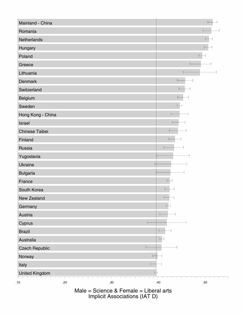
To illustrate the variation in implicit stereotypes beyond the 34 TIMSS nations, we used the complete data set and calculated the mean implicit stereotype among citizens of all available nations. Effects for 61 nations with samples greater than 100 are illustrated in Figure S1. All 61 nations evidenced a mean implicit gender‐science stereotype associating male with science and female with liberal arts more than the reverse. The strength of that association varied substantially across nations. If more of these nations participate in TIMSS or other standardized exams in the future, it will offer an opportunity to replicate and extend these findings.
Magnitude of implicit gender‐science stereotyping for 61 nations (N’s > 100) from data collected at Project Implicit websites (https://implicit.harvard.edu/). Higher positive values indicate stronger associations of male with science and female with liberal arts compared to male with liberal arts and female with science. The reference line is the mean implicit stereotyping effect across nations.
Weighted Regression Analysis Strategy
Because the Project Implicit national citizenship sample sizes varied so widely across the 34 nations involved in the TIMSS testing, analyses were weighted so that the more reliable estimates from larger samples, e.g., Australia with n = 8194, carried more weight than those from smaller samples, e.g., Moldova with n=15. On the other hand, the weighting needed to moderate the leverage of the huge U.S. sample, including more than 80% of the data. To accomplish these goals, we constructed inverse variance weights based on standard errors as opposed to sample sizes. For the IAT weights, we further log‐transformed the weights so as to attenuate the impact of the U.S., while no such transformation was necessary for the TIMSS data. Finally, as the IAT and TIMSS weights were uncorrelated, we averaged them to arrive at a single weighting variable for each IAT‐TIMSS analysis.
Example of SPSS syntax for weighting *weights based on IAT data . COMPUTE IAT_weight = (1 / (IAT_se)**2) . COMPUTE log_IAT_weight = LN(1 / (IAT_se)**2) . *weights based on TIMSS data . COMPUTE TIMSS03_sci_weight = 100 / (BOYSsciSE03 + GIRLSsciSE03)**2 . COMPUTE TIMSS99_sci_weight = 100 / (BOYSsciSE99 + GIRLSsciSE99)**2 . COMPUTE TIMSS03_math_weight = 100 / (BOYSmathSE03 + GIRLSmathSE03)**2 . COMPUTE TIMSS99_math_weight = 100 / (BOYSmathSE99 + GIRLSmathSE99)**2 . *Compute weights combining IAT and TIMSS . *Compute averaged weights. Start by getting means of the above weights * to allow computation of new weights with preserved zero points on scales * shrunk or stretched so that the weights being averaged have means = 1.0. COMPUTE DUMMY = 1 . AGGREGATE OUTFILE = * MODE = ADDVARIABLES / BREAK = DUMMY / Mn_sci03 Mn_sci99 Mn_math03 Mn_math99 Mn_IAT = MEAN(TIMSS03_sci_weight TIMSS99_sci_weight TIMSS03_math_weight TIMSS99_math_weight log_IAT_weight) . COMPUTE combined_03_sci_weight = MEAN(log_IAT_weight/(Mn_IAT), TIMSS03_sci_weight/(Mn_sci03) ) . COMPUTE combined_99_sci_weight = MEAN(log_IAT_weight/(Mn_IAT), TIMSS99_sci_weight/(Mn_sci99) ) . COMPUTE combined_03_math_weight = MEAN(log_IAT_weight/(Mn_IAT), TIMSS03_math_weight/(Mn_math03) ) . COMPUTE combined_99_math_weight = MEAN(log_IAT_weight/(Mn_IAT), TIMSS99_math_weight/(Mn_math99) ) . EXECUTE .
Example of SAS syntax for weighting DATA web.hastimss; SET web.hastimss; *weights based on IAT data; IAT_weight = (1 / (IAT_se)**2) ; log_IAT_weight = LOG(1 / (IAT_se)**2) ; *weights based on TIMSS data; TIMSS03_sci_weight = 100 / (BOYSsciSE03 + GIRLSsciSE03)**2 ; TIMSS99_sci_weight = 100 / (BOYSsciSE99 + GIRLSsciSE99)**2 ; TIMSS03_math_weight = 100 / (BOYSmathSE03 + GIRLSmathSE03)**2 ; TIMSS99_math_weight = 100 / (BOYSmathSE99 + GIRLSmathSE99)**2 ; RUN; /* Compute averaged weights. Start by getting means of the above weights to allow computation of new weights with preserved zero points on scales shrunk or stretched so that the weights being averaged have means = 1.0 */ PROC MEANS NOPRINT DATA = web.hastimss; VAR TIMSS03_sci_weight TIMSS03_math_weight TIMSS99_sci_weight TIMSS99_math_weight log_IAT_weight; OUTPUT OUT=meandat (DROP=_TYPE_ _FREQ_) MEAN=Mn_sci03 Mn_math03 Mn_sci99 Mn_math99 Mn_IAT Mn_raceIAT Mn_ageIAT; PROC PRINT DATA = meandat; RUN ; DATA meansub (DROP=i); IF _N_ = 1 THEN SET meandat; SET web.hastimss; ARRAY means(5) Mn_sci03 Mn_math03 Mn_sci99 Mn_math99 Mn_IAT; DO i = 1 TO 5; END; RUN; DATA web.hasTIMSS; SET meansub; RUN; /* Compute weights combining IAT and TIMSS */ DATA web.hastimss; SET web.hastimss; combined_03_sci_weight = ((log_IAT_weight/Mn_IAT) + (TIMSS03_sci_weight/Mn_sci03))/2; combined_99_sci_weight = ((log_IAT_weight/Mn_IAT) + (TIMSS99_sci_weight/Mn_sci99))/2; combined_03_math_weight = ((log_IAT_weight/Mn_IAT) + (TIMSS03_math_weight/Mn_math03))/2; combined_99_math_weight = ((log_IAT_weight/Mn_IAT) + (TIMSS99_math_weight/Mn_math99))/2; PROC PRINT; VAR countrycitzn combined_03_sci_weight combined_99_sci_weight combined_03_math_weight combined_99_math_weight; RUN;
Regression Analyses
Unless otherwise noted, all analyses are weighted by the respective inverse variances of the given IAT and TIMSS DVs. All variables used as predictors are country‐level and standardized within the set of 34 TIMSS countries to a mean of zero and variance of one. Unstandardized statistics are shown for each country in Table S1 and some key unweighted correlations are shown in Table S2.
corrIATexpsci 6.3 3.5 1.8 0.09percent male -1.9 2.0 -1.0 0.35
age mean 4.3 2.2 2.0 0.07GDPpc -0.8 2.3 -0.4 0.72
GGIindex -3.4 2.2 -1.6 0.13
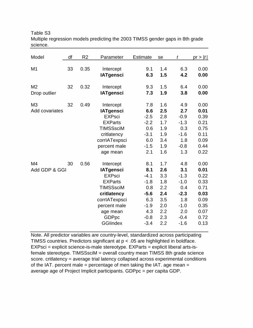
Multiple regression models predicting the 2003 TIMSS gender gaps in 8th grade science.
Note. All predictor variables are country-level, standardized across participating TIMSS countries. Predictors significant at p < .05 are highlighted in boldface. EXPsci = explicit science-is-male stereotype. EXParts = explicit liberal arts-is-female stereotype. TIMSSsciM = overall country mean TIMSS 8th grade science score. critlatency = average trial latency collapsed across experimental conditions of the IAT. percent male = percentage of men taking the IAT. age mean = average age of Project Implicit participants. GDPpc = per capita GDP.
Predicting the 2003 TIMSS 8th Grade Science Gender Gap
Table S3 is a summary of the results from the progression of multiple regression models described in the paper. Model M1 includes only country‐mean gender‐science IAT as a predictor of the 2003 8th grade TIMSS gender gap. After regression diagnostic analyses (see below) identified an extreme outlier for leverage on the regression, the model (M2) was re‐estimated without this observation. With the outlier still excluded, Model M3 adds covariates derived from Project Implicit and TIMSS data, and Model M4 adds the additional covariates of per capita GDP and Gender Gap Index. All model statistics can be viewed at http://briannosek.com/papers/timss/ST3.GLM.8thscidif03.html.
(5) Explicit LA stereotype -0.12 -0.11 0.00 0.13 1
(6) Percentage male 0.08 0.27 0.10 0.40 0.11 1
(7) Age 0.22 0.31 0.17 0.26 -0.11 0.31 1
TABLE S2Unweighted correlations between TIMSS 2003 8th-grade science and math sex differences in 34 countries and by-citizenship-means of stereotype and demographic variables collected through Project Implicit.
Note. T03 = TIMSS 2003, S = Science, M = Math, LA = Liberal Arts. Implicit stereotype measured by a gender-science-liberal arts Implicit Association Test and indexed by a D score effect size. Explicit stereotypes measured by 5- or 7-pt likert scales and standardized within scale type. Coefficients in boldface are significant, p < .05.
Predicting the 2003 TIMSS 8th Grade Math Gender Gap
The same pattern of consistent predictive utility for the IAT was found for the 2003 math gender gaps: http://briannosek.com/papers/timss/ST4.GLM.8thmathdif03.html
Predicting the 1999 TIMSS 8th Grade Science and Math Gender Gaps
As noted in the paper, with two outliers deleted, the gender‐science IAT as a lone predictor remained significantly related to the 1999 science gender gap, but did not persist as a unique predictor when the nine covariates were added to the regression model: http://briannosek.com/papers/timss/ST5.GLM.8thscidif99.html. For the 1999 math gap, exclusion of the one outlying country eliminated the significant relation with implicit stereotyping: http://briannosek.com/papers/timss/ST6.GLM.8thmathdif99.html.
The unweighted regressions of the four dependent variables, TIMSS science and math gender gaps in 2003 and 1999, on implicit stereotyping, yield results similar to those obtained with weighting. That is, the effect of national implicit stereotype was significant at p < .05 for both science outcomes and for math in 2003, but not for math in 1999 (p = .08). Regression diagnostics identified Tunisia as an outlier in all models, and Jordan for the 2003 science model in addition to the 1999 one identified in the weighted analysis. These two countries are among the three smallest IAT samples (both < 40), and Moldova, the smallest at n=15, was next highest in leverage in each model. When the regression models were refit without these outliers, implicit stereotype was a significant predictor (p < .05) of three of the four TIMSS gender gaps, science and math in 2003, science in 1999, just as in the weighted analyses: http://briannosek.com/papers/timss/ST7.GLM.allDVs.unweighted.html.
Regression Diagnostics for Influential Observations
Testing whether any observations are exerting undue influence on a regression analysis is always important, and especially when sample sizes are small. Following Cohen et al. (10), we calculated studentized residuals, leverage, Cook’s D and DFITS statistics for each of the four primary regression analyses, both weighted and unweighted.
We calculated, for the 2003 (N=34) and 1999 (N=29) regressions, respectively, the following thresholds for each index according to Cohen et al. (2003) guidelines for small sample regression diagnostics (p. 397‐404): studentized residuals (Bonferroni procedure) > |3.46|,|3.48|; leverage > .18, .21; Cook’s D (F distribution procedure) > .71 for both; DFITS > |1| for both. In the weighted regressions with gender‐science IAT as the sole predictor of each of the four focal TIMSS 8th grade gender differences (2003 science and math, 1999 science and math), Tunisia emerged as an extreme leverage outlier in each, and also on Cook’s D and DFITS for both math outcomes, while Jordan exceeded the DFITS threshold for the 1999 science regression. In the unweighted regressions, Tunisia, again, was an outlier on at least one index in all four models, and Jordan, in addition to outlying in the 1999 science model, was also outlying on DFITS for the 2003 science model. While we have no reason to suspect that these observations are spurious, as noted in the paper we have excluded them and re‐fit all regressions so as to increase our confidence in the replicability of our results.
Diagnostic statistics for all models regressing TIMSS outcomes on the IAT, weighted and unweighted, are here:
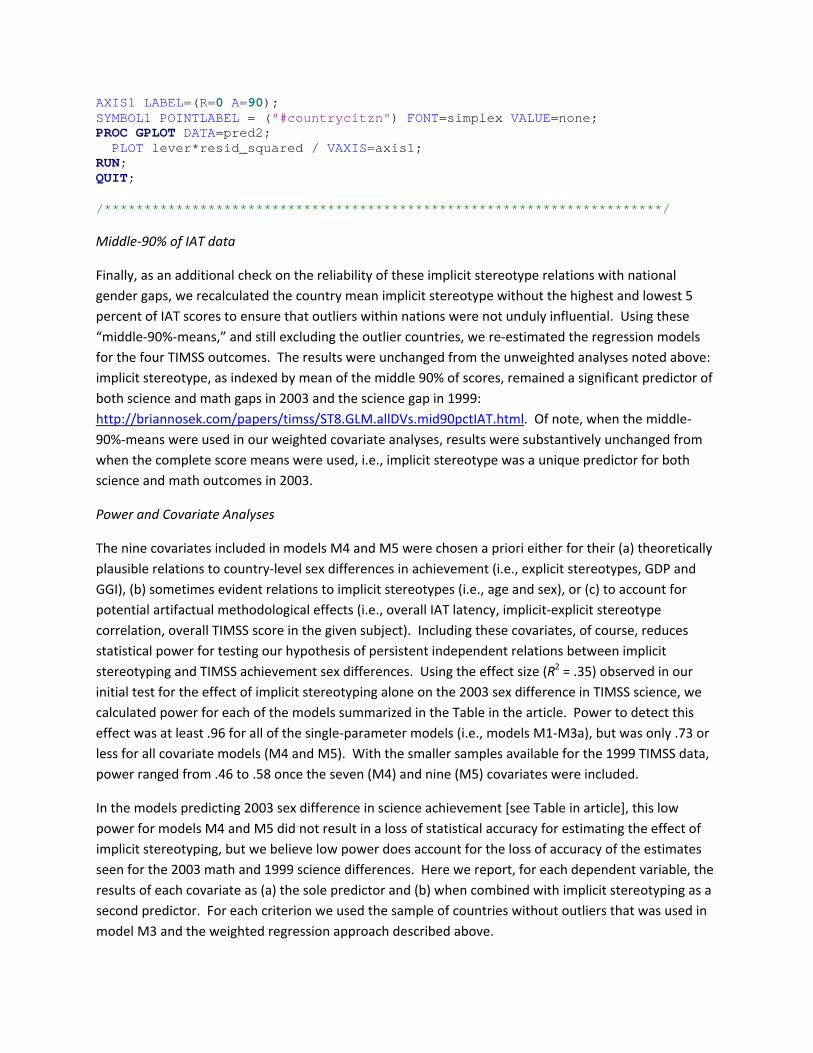
Finally, as an additional check on the reliability of these implicit stereotype relations with national gender gaps, we recalculated the country mean implicit stereotype without the highest and lowest 5 percent of IAT scores to ensure that outliers within nations were not unduly influential. Using these “middle‐90%‐means,” and still excluding the outlier countries, we re‐estimated the regression models for the four TIMSS outcomes. The results were unchanged from the unweighted analyses noted above: implicit stereotype, as indexed by mean of the middle 90% of scores, remained a significant predictor of both science and math gaps in 2003 and the science gap in 1999: http://briannosek.com/papers/timss/ST8.GLM.allDVs.mid90pctIAT.html. Of note, when the middle‐90%‐means were used in our weighted covariate analyses, results were substantively unchanged from when the complete score means were used, i.e., implicit stereotype was a unique predictor for both science and math outcomes in 2003.
Power and Covariate Analyses
The nine covariates included in models M4 and M5 were chosen a priori either for their (a) theoretically plausible relations to country‐level sex differences in achievement (i.e., explicit stereotypes, GDP and GGI), (b) sometimes evident relations to implicit stereotypes (i.e., age and sex), or (c) to account for potential artifactual methodological effects (i.e., overall IAT latency, implicit‐explicit stereotype correlation, overall TIMSS score in the given subject). Including these covariates, of course, reduces statistical power for testing our hypothesis of persistent independent relations between implicit stereotyping and TIMSS achievement sex differences. Using the effect size (R2 = .35) observed in our initial test for the effect of implicit stereotyping alone on the 2003 sex difference in TIMSS science, we calculated power for each of the models summarized in the Table in the article. Power to detect this effect was at least .96 for all of the single‐parameter models (i.e., models M1‐M3a), but was only .73 or less for all covariate models (M4 and M5). With the smaller samples available for the 1999 TIMSS data, power ranged from .46 to .58 once the seven (M4) and nine (M5) covariates were included.
In the models predicting 2003 sex difference in science achievement [see Table in article], this low power for models M4 and M5 did not result in a loss of statistical accuracy for estimating the effect of implicit stereotyping, but we believe low power does account for the loss of accuracy of the estimates seen for the 2003 math and 1999 science differences. Here we report, for each dependent variable, the results of each covariate as (a) the sole predictor and (b) when combined with implicit stereotyping as a second predictor. For each criterion we used the sample of countries without outliers that was used in model M3 and the weighted regression approach described above.
Overall, out of 36 single predictor models (nine covariate variables predicting, in turn, the four criteria) only two yielded statistically significant relationships at p < .05: 2003 science difference regressed on explicit science stereotype, and 1999 science difference regressed on Gender Gap Index (GGI). For the 2003 science and math criteria, when implicit stereotyping was added as a second predictor in each model, its independent effect remained statistically significant in every case (lowest standardized effect estimates were 0.58 and 0.48, respectively, for science and math outcomes). For the 1999 science criterion, however, despite the lack of significant prediction for all covariates except GGI, the coupling with implicit stereotyping was sufficient to reduce to non‐significance the estimate of the implicit stereotyping effect for 7 of 9 models. This was the case even though the lowest estimated effect size for implicit stereotyping (when combined in a model with explicit stereotyping) was a third of a standard deviation (standardized effect = 0.33, compared with 0.43 when implicit stereotyping was sole predictor). Thus, we believe low power, and not lack of considerable independent effect of implicit stereotyping, is the best explanation for non‐significant effects when covariates were added to the prediction of 2003 math (on model M4) and 1999 science criteria (M4 and M5).
2003 science criterion: Of the nine covariates, only explicit stereotype by itself was a significant predictor. Its effect was reduced to non‐significance with inclusion of implicit stereotyping, and implicit stereotyping was a significant predictor in every case when added to models with single covariates. http://briannosek.com/papers/timss/GLM.8thscidif03.covariatesimpact.html
2003 math criterion: None of nine covariates alone was a significant predictor. Implicit stereotyping was significant in every case when added to models with single covariates. http://briannosek.com/papers/timss/GLM.8thmathdif03.covariatesimpact.html
1999 science criterion: Of the nine covariates, only GGI by itself was a significant predictor. The estimated effect of implicit stereotyping, when added to each model as a second predictor, was not statistically significant in 7 of 9 models, even though its lowest standardized effect was a substantial 0.33. Of those added in M5, GDP was ns alone, and reduced IAT to ns, but GGI was significant (similar to Guiso 8), and IAT remained independently significant. http://briannosek.com/papers/timss/GLM.8thscidif99.covariatesimpact.html
1999 math criterion: None of nine covariates alone was a significant predictor. Implicit stereotyping was not a significant predictor in any model when added as second variable. http://briannosek.com/papers/timss/GLM.8thmathdif99.covariatesimpact.html
Covariates and Reversed Causal Direction
A reviewer suggested that, in keeping with our emphasis that stereotyping and sex differences in achievement are likely bi‐directional in influence, and especially since the 1999 TIMSS administration preceded our implicit stereotyping data collection, we examine the effects of our covariates with a reversed modeling strategy (i.e., predict stereotyping from sex differences instead of sex differences from stereotyping).
When replicating models M4 and M5 in this manner, with country‐level implicit stereotyping as the DV in each case, we found the same pattern of results for the effect of the covariates on the relation between implicit stereotyping and the given sex difference in TIMSS achievement. That is, for the effect of TIMSS science difference in 2003, a significant relation remained for both models M4 and M5; the effect of TIMSS math 2003 was non‐significant (p = .06) for M4 and significant for M5; and neither TIMSS science nor math in 1999 was significant in models M4 and M5.
We took this occasion, however, to fit some post‐hoc exploratory models for the prediction of implicit stereotyping based on observed variable correlations (see correlation tables and exploratory model results in the links below). The same three variables—TIMSS achievement sex difference, TIMSS overall score, and explicit gender‐science stereotyping—were correlated at p < .05 with implicit stereotyping for three of the four groups of variables (science and math in 2003, and science in 1999; for the 1999 math group, only explicit gender‐science stereotyping was significantly related to implicit stereotyping). Therefore, we entered these three variables as predictors in a simultaneous multiple regression model for implicit stereotyping in each of the four TIMSS groupings. The independent effect of TIMSS sex difference on implicit stereotyping remained significant, or nearly so, for all three of the models where it was a significant solo predictor: Science 2003, p < .05, Math 2003, p = .06., and Science 1999, p < .05. None of the other variables were independently significant at p < .08.
Other TIMSS Outcomes: Grade 8 in 1995 and Grade 4 in 2003 and 1995
Eighth graders were also measured by TIMSS in 1995, but by‐gender performance was only reported for N = 22 countries. Fourth grade performance was reported for 2003 and 1995, but with by‐gender performance for only N = 15 countries. Despite the very small samples, we estimated regressions of science and math gender gaps on implicit gender‐science stereotyping for each of these samples. None elicited significant effects. Because of the small samples, we are reluctant to make a substantive conclusion that 4th grade science and math performance is not reflected in national indicators of implicit stereotypes.
A substantive explanation for variation in correlation strengths between implicit stereotypes and different years of TIMSS study administration?
In the article, we suggested that that the most plausible explanation for variation in the significant effects, and robustness to our conservative tests was low statistical power. Though plausible, that is not the only possible explanation. Figure S2 includes 1995 TIMSS data with 1999 and 2003 and suggests a potential substantive explanation for the weaker relation between national implicit stereotyping, measured between 2000‐2008, and earlier, as opposed to more concurrent, measures of sex differences in performance. Specifically, Figure S2 displays, roughly in temporal order, the TIMSS sex differences in
science for 1995, 1999, and 2003, and implicit gender‐science stereotyping [math statistics are included at http://briannosek.com/papers/timss/CORR.IATandTIMSS039995.html].
The changing TIMSS mean sex difference reflects real change in addition to that caused by shifts in sample composition. For example, the 1995 and 1999 means for the 17 nations measured in each of those years are 19 and 17, respectively, while those for the 22 nations measured in both 1995 and 2003 are 19 and 11. This observation, combined with the changing TIMSS correlations, suggests that the national science sex differences are changing over time. The systematically increasing correlations between these differences and implicit stereotyping is suggestive of a closer temporal relation between these variables. Without concurrent measurement of implicit stereotypes in 1995 and 1999, these observations get us no closer to a causal inference, but they suggest a potentially more immediate relationship between the environment and implicit biases. Because of the small samples and the post‐hoc nature of this observation, we are reluctant to draw any definitive conclusions. At minimum, these data provide for intriguing speculation that there are temporal dynamics between implicit stereotypes and actual sex differences in performance.
Discriminant Validity Studies
Neither implicit racial attitudes nor implicit age attitudes predict gender differences in TIMSS performance
Even if implausible, selection factors and construct‐irrelevant influences on the IAT could be alternative explanations for the observed relationship between gender differences in TIMSS performance and implicit gender‐science stereotyping. To increase our confidence that the effect is a function of implicit gender stereotypes and not an irrelevant influence, we replicated the analysis using, in turn, country‐mean implicit racial and age attitudes – content domains that should not predict gender differences in TIMSS performance.
Race Attitude Participants
A total of 527,533 participants from 34 nations were included in the dataset for comparison with TIMSS. The median country sample n = 412.
Age Attitude Participants
A total of 209,984 participants from the 34 TIMSS nations were included with median country sample n = 446.
Materials
Implicit Association Tests. The race IAT measured association strengths between Black and White faces and good and bad words (Nosek, Smyth, et al., 2007), while the age IAT measured association strengths between Young and Old faces and good and bad words (Nosek, Smyth, et al., 2007). Otherwise, the measures were the same as the gender‐science IAT.
The procedure was identical to the gender‐science task except that the IAT and self‐report items referred to racial or age attitudes rather than gender stereotypes. The procedure can be self‐administered at https://implicit.harvard.edu/.
Analysis
We refit the full multiple regression model for each of the 2003 and 1999 TIMSS gender gaps, including the same nine covariates, but substituting, in turn, the national estimates of implicit race attitude and implicit age attitude in place of the implicit gender‐science stereotype. The race and age models were weighted with the inverse variances of the race and age IATs, respectively, in the same way that the gender‐science models were weighted.
Results
The national estimate of implicit race attitude did not account for unique variance in any of the four models (all p’s > .43). Complete model statistics are here http://briannosek.com/papers/timss/ST17.RaceIATanalysis.covariates.html. Likewise, country‐mean implicit age attitude did not contribute uniquely to the prediction of science and math gender differences (all p’s > .28) http://briannosek.com/papers/timss/ST18.AgeIATanalysis.covariates.html.
These null effects are in contrast with the significant unique effects of the national estimate of implicit gender‐science stereotyping in predicting the 2003 gender gaps in science and math.
1. TIMSS Appendices (2003) TIMSS science and math test score data by‐country, by‐sex, Appendix C. Retrieved March 31 from http://nces.ed.gov/pubs2005/timss03/pdf/timss_appendices.pdf.
2. Greenwald AG, McGhee DE, Schwarz JLK (1998) Measuring individual differences in implicit cognition: The Implicit Association Test. J of Pers and Soc Psychol 74:1464‐1480.
3. Nosek BA, Greenwald AG, Banaji MR (2006) in Social Psychology and the Unconscious: The Automaticity of Higher Mental Processes. ed Bargh JA (Psychology Press, New York), pp. 265‐292.
4. Greenwald AG, Nosek BA, Banaji, MR (2003) Understanding and using the Implicit Association Test: I. An improved scoring algorithm. J of Pers and Soc Psychol 85: 197‐216.
5. Nosek BA, Greenwald AG, Banaji MR (2005) Understanding and using the Implicit Association Test: II. Method variables and construct validity. Pers and Soc Psychol Bul 31: 166‐180.
6. Nosek BA et al (2007) Pervasiveness and correlates of implicit attitudes and stereotypes. Euro Rev of Soc Psychol 18: 36‐88.
7. Central Intelligence Agency (2008) The World Factbook. Retrieved July 17 from https://www.cia.gov/library/publications/the‐world‐factbook/rankorder/2004rank.html.
8. Guiso L, Monte F, Sapienza P, Zingales L (2008) Culture, gender and math. Science 320:1164‐1165.
9. World Economic Forum (2006) Gender Gap Index (GGI) 2006 data retrieved July 19, 2008 from http://www.weforum.org/en/Communities/Women%20Leaders%20and%20Gender%20Parity/GenderGapNetwork/index.htm.
10. Cohen J, Cohen P, West SG, Aiken LS (2003) Applied multiple regression/correlation analysis for the behavioral sciences, (Lawrence Erlbaum Associates, Mahway, NJ).
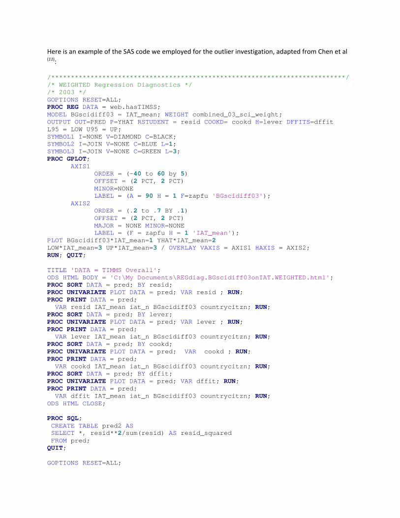
11. Chen X, Ender P, Mitchell M, Wells C (2008) Regression Diagnostics. Retrieved March 31 from http://www.ats.ucla.edu/stat/sas/webbooks/reg/chapter2/sasreg2.htm.
Magnitude of implicit gender‐science stereotyping for 61 nations (N’s > 100) from data collected at Project Implicit websites (https://implicit.harvard.edu/). Higher positive values indicate stronger associations of male with science and female with liberal arts compared to male with liberal arts and female with science. The reference line is the mean implicit stereotyping effect across nations.
Figure S2
Diagram of (a) mean TIMSS 8th‐grade science gender gaps for 1995, 1999, and 2003, (b) correlations with one another, and (c) with the national indicator of implicit gender‐science stereotyping (IAT) derived from tests administered between 2000 and 2008.