Abstract We present a computational method for the opti-mization of nanostructures, where our specific interest is incapturing and elucidating surface stress and surface elas-tic effects on the optimal nanodesign. XFEM is used tosolve the nanomechanical boundary value problem, whichinvolves a discontinuity in the strain field and the presence ofsurface effects along the interface. The boundary of the nano-structure is implicitly represented by a level set function,which is considered as the design variable in the optimiza-tion process. Two objective functions, minimizing the totalpotential energy of a nanostructure subjected to a mater-ial volume constraint and minimizing the least square errorcompared to a target displacement, are chosen for the numer-ical examples. We present results of optimal topologies of ananobeam subject to cantilever and fixed boundary condi-tions. The numerical examples demonstrate the importanceof size and aspect ratio in determining how surface effectsimpact the optimized topology of nanobeams.
1 Institute of Structural Mechanics, Bauhaus-UniversitätWeimar, Marienstraße 15, 99423 Weimar, Germany
2 Department of Mechanical Engineering, Boston University,730 Commonwealth Avenue, ENA 212, Boston, MA 02215,USA
3 School of Civil, Environmental and ArchitecturalEngineering, Korea university, Seoul, Republic of Korea
Keywords Nanomaterials · Surface effects · Shapeoptimization · Extended finite element method (XFEM) ·Level set method
1 Introduction
Due to their unique physical properties [1,2], nanostruc-tures have recently attracted significant attention from thescientific community. In addition to their electronic, thermaland optical properties, nanostructures can exhibit mechani-cal behavior and properties that are superior to those of thecorresponding bulk material. The underlying physical mech-anism for the changes in the mechanical, and other physicalproperties with decreasing structure size, is the increasingsignificance of surface effects, which is due to increasingsurface area to volume ratio [3].
The physical origin of the surface effects is that atomsat the surfaces of a material have fewer bonding neigh-bors than atoms that lie within the material bulk [4]. Thisso-called undercoordination of the surface atoms causesthem to exhibit different elastic properties than atoms inthe bulk, which can lead to either stiffening or softeningof the nanostructure, as described by Zhou and Huang [5]and recently reviewed by Park et al [6]. Surface effectsalso have a first order effect on the deformation mech-anisms and plasticity in nanostructures, as illustrated invarious works [7–9] and recently summarized byWeinbergerand Cai [10]. Therefore, it is critical to consider surfaceeffects when discussing the mechanical behavior and prop-erties of nanomaterials, particularly when any characteristicdimension of the nanostructure is smaller than about 100nm [6].
These unique mechanical properties have motivatedresearchers to develop computational approaches that capture
these surface effects based on either linear or nonlin-ear continuum theories. For example, many computationalapproaches [11–14] are based on the well-known Gurtin–Murdoch linear surface elasticity theory [15], which consid-ers the surface to be an entity of zero thickness that has itsown elastic properties that are distinct from the bulk. Otherapproaches have considered a bulk plus surface ansatz ofvarious forms incorporating finite deformation kinematics.The approaches not bound on the Gurtin–Murdoch frame-work include thework bySteinmann and co-workers [16,17],and the surface Cauchy–Born approach of Park and co-workers [18–20]. The interested reader is also referred tothe recent review of Javili et al [21].
However,most theoretical and computational studies havefocused on determining how surface effects impact spe-cific mechanical properties, i.e. the Young’s modulus [6],plastic deformation mechanisms [7,10], resonant frequen-cies [22,23], bending response [24,25], and more generallythemechanical response of nanostructures such as nanowiresor nanobeams. What has not been done to-date is to investi-gate how surface effects impact the topology of nanostruc-tures within the concept of optimally performing structures.This topic has a significant history and literature for bulkmaterials [26–28], but has not been studied for surface-dominated nanostructures.
The objective of this work is therefore to present a numer-ical method that can be used to study the optimization ofnanostructures, while accounting for the critical physics ofinterest, that of nanoscale surface effects. The formulationis general, and can be applied to different materials suchas FCC metals or silicon so long as the relevant surfaceelastic constants are known. This is done through a cou-pling of the extended finite element method (XFEM) [29]and the level set method [27]. By using XFEM to solvethe nanomechanical boundary value problem including sur-face effects based on Gurtin–Murdoch surface elasticitytheory [11,14,15], we are able to maintain a fixed back-ground FE mesh while only the structural topology varies.The level set method (LSM) in which the front velocityis derived from a shape sensitivity analysis by solving anadjoint problem is based on the ideas proposed by Allaire etal.[27].
The outline of the paper is as follows. In Sect. 2, based onGurtin–Murdoch surface elasticity theory [15], the contin-uum model for an elastic solid considering surface effectsis presented. Section 3 illustrates the LSM for structuraloptimization. In Sect. 4, the objective functions and themate-rial derivative for shape sensitivity analysis are presented. Abrief overview on the XFEM formulation is given in Sect. 5followed by numerical examples in Sect. 6, and finally con-cluding remarks.
2 Continuum model
We consider an elastic solid � with a material surface∂�. According to continuum theory of elastic material sur-faces [15], the equilibrium equations for a nanostructure canbe written as:
∇ · σ + b = 0 in� (1)
∇s · σ s + [σ · n] = 0 on� (2)
where the first equation refers to bulk equilibrium and thesecond equation refers to the generalized Young-LaplaceEq. [15] resulting from mechanical equilibrium on the sur-face. In the above equations, σ represents bulk Cauchy stresstensor, b represents the body force vector, σ s denotes the sur-face stress tensor, n is the outward unit normal vector to �,and∇s ·σ s = ∇σ s : P.HereP is the tangential projection ten-sor to� at x ∈ � which is defined as P(x) = I−n(x)⊗n(x),I is the second order unit tensor. Γ is the boundary of thedomain Ω . Furthermore, the boundary conditions are givenby
σ · n = t on�N
u = u on�D(3)
where t and u are the prescribed traction and displacement,respectively, and �N and �D are the Neumann and Dirichletboundaries. The bulk strain tensor ε and surface strain tensorεs are written as
ε = 1
2
(∇u + (∇u)T)
(4)
εs = P · ε · P (5)
where u is the displacement vector. Assuming a linear elas-tic bulk material and an isotropic linear elastic surface, theconstitutive equations for the bulk and surface can be writtenas
σ = Cbulk : ε (6)
σ s = ∂γ
∂εs(7)
where γ is the surface energy density given by
γ = γ0 + τ s : εs + 1
2εs : Cs : εs (8)
where γ0 is the surface free energy density that exists evenwhen εs = 0, and τ s = τsP is the surface residual stresstensor. By substituting Eq. 8 into Eq. 7, σ s can be obtainedby
123
Comput Mech (2015) 56:97–112 99
σ s = τ s + Cs : εs (9)
In the above equations, Cbulk and Cs are the fourth-order
elastic stiffness tensors associated with the bulk and surface,respectively, and are defined as
Cbulki jkl = λδi jδkl + μ
(δikδ jl + δilδ jk
)(10)
Csi jkl = λs Pi j Pkl + μs
(Pik Pjl + Pil Pjk
)(11)
where λ and μ, and λs and μs are the Lamé constants of thebulk and surface, respectively.
It should be noted that the surface is considered as a specialcase of a coherent imperfect interface between two materialswhen one of them exists in a vacuumphase [12]. It is assumedthat the surface adheres to the bulk and therefore we have:
�u� = 0 (i.e.) (u)+ − (u)− = 0 on� (12)
where �.� denotes the jump across the interface.Having defined the constitutive and field equations, we
derive theweak formof the boundary value problembased ontheprinciple of stationarypotential energy.The total potentialenergy Π of the system is given by
Π = Πbulk + Πs − Πext (13)
where Πbulk , Πs , and Πext represent the bulk elastic strainenergy, surface elastic energy and thework of external forces,respectively, which are given by
Πbulk = 1
2
∫
Ω
ε : Cbulk : ε dΩ (14)
Πs =∫
Γ
γ dΓ (15)
Πext =∫
ΓN
u · t dΓ +∫
Ω
u · b dΩ (16)
The stationary condition of Eq. 13 is given by
DδuΠ = 0 (17)
where Dmϒ is the directional derivative (or Gâteaux deriv-ative) of the functional ϒ in the direction m. Applying thestationary condition, the weak form of the equilibrium equa-tions can be obtained by finding u ∈ {
u = u on�D,u ∈H1(Ω)
}such that
∫
Ω
ε(u) : Cbulk : ε(δu) dΩ +∫
Γ
εs(u) : Cs : εs(δu) dΓ
= −∫
Γ
τ s : εs(δu) dΓ +∫
ΓN
δu · t dΓ +∫
Ω
δu · b dΩ
(18)
for all δu ∈ {δu = 0 on�D, δu ∈ H1(Ω)
}. This weak
form can be written in a simplified form as
a(u, δu) + as(u, δu) = −ls(δu) + l(δu) (19)
where the bilinear functionals a(u, δu) and as(u, δu), andlinear functionals l(δu) and ls(δu) are defined as
a(u, δu) =∫
Ωc(u, δu) dΩ =
∫
Ωε(u) : Cbulk : ε(δu) dΩ
as(u, δu) =∫
∂Ωcs(u, δu) dΓ =
∫
∂Ωεs(u) : Cs : εs(δu) dΓ
l(δu) =∫
∂ΩN
δu · t dΓ +∫
Ωδu · b dΩ
ls(δu) =∫
∂Ωτ s : εs(δu) dΓ
(20)
3 Level set method
The LSM, which was first introduced by Osher and Sethian[30] for tracking moving interfaces, has been extensivelyapplied to many different research fields such as imageprocessing, computer graphics, fluid mechanics, and crackpropagation over the past three decades. The first researchwork on incorporating the LSM [30] in structural shapeand topology optimization was performed by Sethian andWiegmann [31]. They used the LSM to represent the designstructure and to alter the design shape based on a Von Misesequivalent stress criterion. Later, Osher and Santosa [32],Allaire et al. [27], and Wang et al. [33] independently pro-posed a new class of structural optimization method basedon a combination of the level set method with the shape sen-sitivity analysis framework. The main idea of this method isto model the process of structural optimization via a scalarlevel set function which dynamically changes in time. There-fore, the evolution of the design shape is governed by theHamilton–Jacobi (H–J) partial differential equation (PDE)in which the front speed (or velocity vector) links the H–Jequation with the shape sensitivity analysis. This method isusually called conventional LSM and is widely used in struc-tural optimization [33,34].Wenote that there is no nucleationmechanism for new holes in this method. However the level-set method can easily handle topology changes, i.e. mergingor vanishing of holes, and thus this algorithm can be used toperform topology optimization.
We assume D ⊂ Rd (d = 2 or 3) as the whole structural
shape and topology design domain including all admissibleshapes Ω , i.e. Ω ⊂ D. A level set function (x) whichpartitions the design domain D into three parts, i.e. the solid,void and the boundary which are defined as
123
100 Comput Mech (2015) 56:97–112
Solid : (x) < 0 ∀x ∈ � \ ∂�
Boundary : (x) = 0 ∀x ∈ ∂� ∩ D
Void : (x) > 0 ∀x ∈ D \ �
(21)
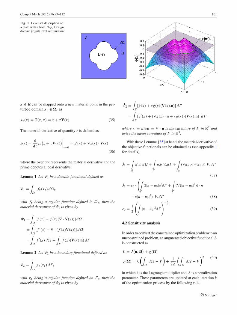
The basic idea of the LSM for structural optimization is todescribe the structural design boundary �(x) implicitly bythe zero level set of a higher dimensional level set function(see Fig. 1):
�(x) ={x ∈ R
d |(x) = 0}
(22)
To allow the design boundary for a dynamic evolution in theoptimization process, we introduce t as a fictitious time. Thusthe dynamic design boundary is defined as
�(t) ={x(t) ∈ R
d |(x(t), t
) = 0}
(23)
By differentiating{
(x(t), t
) = 0}with respect to time1,
we obtain the well-known Hamilton–Jacobi PDE
∂(x(t), t)∂t
+ ∇(x(t), t) · V = 0 (24)
where V = dxdt denotes the velocity vector of the design
boundary. This equation can be further written consideringthe unit outward normal n = ∇
|∇| to the boundary and nor-mal component of velocity vector Vn = V · n,∂
∂t+ Vn|∇| = 0 (25)
By solving this Hamilton–Jacobi equation, the level set func-tion and consequently the structural design boundary isupdated during the optimization process. It should be notedthat here Vn is a quantity that links the LSM to the shapedesign sensitivity analysis [33].
The Hamilton–Jacobi equations usually do not admitsmooth solutions. Existence and uniqueness are achievedin the framework of viscosity solutions which provide aconvenient definition of the generalized shape motion. Thediscrete solutionof theH–J equation is obtainedby an explicitfirst-order upwind scheme [27]. The level set function is reg-ularized periodically by solving
∂
∂t+ sign (0)
(‖∇∥∥ − 1) = 0. (26)
Solving this equation gives a signed distance function withrespect to an initial isoline,0. This ensures smoot-her inter-faces and also that the signed distance from the interface can
1 This is the same as taking the material derivative of{(x(t), t) = 0
}.
be used as enrichment values for the nodes whose support iscut by the zero level sets, for the XFEM analysis performedin each iteration.
4 Material derivative approach and sensitivityanalysis
In this work, we consider two objective functions. The firstconsiders the total potential energyof the nanostructure underequilibrium and volume constraints. For this case, the topol-ogy optimization problem can be defined as
Minimize J1(�) =∫
Ω
u · bdΩ +∫
ΓN
u · tdΓ (27)
Subject to∫
Ω
dΩ − V = 0 (28)
a(u, v,�) + as(u, v,�) = −ls(v,�) + l(v,�) (29)
The second is a least square error objective function com-pared to a target displacement, which can be written as
Minimize J2(�) =⎛
⎝∫
Γ
|u − u0|2dΓ
⎞
⎠
12
(30)
Subject to (31)
a(u, v,�
) + as(u, v,�
) = −ls(v,�) + l(v,�
)(32)
Here we assume v = δu and γ0 = 0. To perform shapeoptimization, it is essential to find the relationship betweena variation in design variables and the resulting variationsin cost functional [35] using a sensitivity analysis method.For this purpose, we use the material derivative concept fromcontinuum mechanics.
4.1 Material derivative
Consider an initial structural domain�which is transformedinto a deformed (or perturbed) structural domain �τ in afictitious time τ . This transformation can be viewed as amapping T : x → xτ (x), x ∈ � such that
xτ ≡ T(x, τ )
�τ ≡ T(�, τ )(33)
A design velocity field can be defined as
V(xτ , τ ) ≡ dxτ
dτ= dT(x, τ )
dτ= ∂T(x, τ )
∂τ(34)
Based on the linear Taylor’s series expansion of T(x, τ )
around τ = 0 [35], any material point in the initial domain
123
Comput Mech (2015) 56:97–112 101
Fig. 1 Level set description ofa plate with a hole. (left) Designdomain (right) level set function
x ∈ � can be mapped onto a new material point in the per-turbed domain xτ ∈ �τ as
xτ (x) = T(x, τ ) = x + τV(x) (35)
The material derivative of quantity z is defined as
z(x) = d
dτzτ
(x + τV(x)
)∣∣∣∣τ=0
= z′(x) + ∇z(x) · V(x)
(36)
where the over dot represents the material derivative and theprime denotes a local derivative.
Lemma 1 Let Ψ1 be a domain functional defined as
Ψ1 =∫
Ωτ
fτ (xτ ) dΩτ
with fτ being a regular function defined in Ωτ , then thematerial derivative of Ψ1 is given by
Ψ1 =∫
Ω
[ f (x) + f (x)(∇ · V(x))] dΩ
=∫
Ω
[ f ′(x) + ∇ · ( f (x)V(x))] dΩ
=∫
Ω
f ′(x) dΩ +∫
Γ
f (x)(V(x).n) dΓ
Lemma 2 Let Ψ2 be a boundary functional defined as
Ψ2 =∫
Γτ
gτ (xτ ) dΓτ
with gτ being a regular function defined on Γτ , then thematerial derivative of Ψ2 is given by
Ψ2 =∫
Γ
[g(x) + κg(x)(V(x).n)] dΓ
=∫
Γ
[g′(x) + (∇g(x) · n + κg(x))(V(x).n)] dΓ
where κ = divn = ∇ · n is the curvature of Γ in R2 and
twice the mean curvature of Γ in R3.
With these Lemmas [35] at hand, thematerial derivative ofthe objective functionals can be obtained as (see appendix 1for details),
J1 =∫
Ω
u′.b dΩ +∫
Γ
u.b VndΓ +∫
ΓN
(∇u.t.n + κu.t) VndΓ
(37)
J2 = c0 ·⎛
⎝∫
Γ
2|u − u0|u′dΓ +∫
Γ
(∇(|u − u0|2)) · n
+ κ|u − u0|2)VndΓ (38)
c0 = 1
2
⎛
⎝∫
Γ
|u − u0|2dΓ
⎞
⎠
− 12
(39)
4.2 Sensitivity analysis
In order to convert the constrainedoptimization problem to anunconstrained problem, an augmented objective functional Lis constructed as
L = J(u,�
) + χ(�)
χ(�) = λ
(∫
Ω
dΩ − V
)+ 1
2Λ
(∫
Ω
dΩ − V
)2 (40)
in which λ is the Lagrange multiplier and Λ is a penalizationparameter. These parameters are updated at each iteration kof the optimization process by the following rule
123
102 Comput Mech (2015) 56:97–112
λk+1 = λk + 1
Λk
(∫
Ω
dΩ − V
)
Λk+1 = ζΛk(41)
where ζ ∈ (0, 1) is a constant parameter.The shape derivative of augmented Lagrangian L is
defined as
L ′ = J ′(u,�) + χ ′(�) (42)
J ′ =∫
Γ
G.VndΓ (43)
G = −∫
Γ
ε(u) : Cbulk : ε(w) dΓ
−∫
Γ
κ(Pε(w)P : τ s)dΓ
−∫
Γ
κ(Pε(u)P : Cs : Pε(w)P)dΓ (44)
χ ′(�) =∫
∂Ω
max
{0, λ + 1
Λ
(∫
Ω
dΩ − V
)}Vn dΓ
(45)
Based on the steepest descent direction,
Vn = −∫
Γ
ε(u) : Cbulk : ε(w) dΓ
−∫
Γ
κ(Pε(w)P : τ s)dΓ
−∫
Γ
κ(Pε(u)P : Cs : Pε(w)P)dΓ (46)
J ′ = −∫
Γ
V 2n dΓ ≤ 0 (47)
Velocity extension The normal velocity of the front Vn is tobe extended from the front to the whole design domain inorder to solve the HJ Eq. 25. Different techniques for veloc-ity extension have been proposed in the literature e.g. thenormal, natural, Hilbertian andHelmholtz velocity extensionmethods (see [36] for a review on different velocity extensionstrategies). It is obvious from Eq. 47 that the velocity com-prises two parts, the bulk, Vb and surface terms, Vs . The bulkpart of velocity, Vb can be obtained at each node whereas thesurface part, Vs can be determined only along the surface. Inorder to solve HJ Eq. 25 that is posed throughout the domain,the surface part of velocity Vs is extended by extrapolationto the nodes that belong to the cut elements. The value of thespeed function at the closest point on the surface is assigned
as the extension velocity to the nodal point [37], such thatthe condition Vext = Vn at φ = 0 is satisfied.
5 Extended finite element method
XFEM is a robust numerical approach that enables mod-elling the evolution of discontinuities such as cracks withoutremeshing. It is used to analyze the nanobeams in each step ofthe iterative optimization process, where the XFEM formu-lation for solving nanomechanical boundary value problemsincluding surface effects is based on the work of Farsadet al.[14]. In XFEM, the cracks, voids and material inter-faces are implicitly represented by using level set functions[38,39]. In XFEM, the approximation of the displacementfield in a material with several material subdomains is givenby
uh(X) =∑
i∈INi (X)ui + uenr (48)
uenr =nc∑
N=1
∑
j∈J
N j (X)a(N)j F(X) (49)
where aj is the additional degrees of freedom (DOF) thataccounts for the jump in the strain field, nc denotes the num-ber of material interfaces, and J is the set of all nodes whosesupport is cut by the material interface. In this work, theabsolute enrichment function F(x) [40]
F(X) =∑
I
Ni (X)|φi (X)| − |Ni (x)φi (X)| (50)
is used in order to account for the discontinuous strain fieldalong Γ . The voids are assumed to be filled with a materialthat is 1000 times softer than the stiffness of the nanos-tructure. The usage of a softer material enables the tractionand displacement boundary to intersect with the void bound-ary. The stiffness coefficients are determined by numericalintegration performed over sub triangles on either side ofthe inclusion interface. Substituting the displacement fieldin Eq. 48 to the weak formulation, Eq. 18, the algebraicfinite element equations can be obtained. The expressionsfor a(u, δu), as(u, δu), ls(δu) and l(δu) for an element canbe rewritten using the FE approximation as,
ae(u, δu) = δueT
⎛
⎝∫
Ωe
BT{Cbulk}B dΩe
⎞
⎠ue (51)
aes (u, δu) + les (δu) =∫
Γ e
(Pε(u)P) {Cs} (Pε(δu)P)dΓ e
123
Comput Mech (2015) 56:97–112 103
+∫
Γ e
τ s (Pε(u)P)dΓ e
= δueT
⎛
⎝∫
Γ e
BTMpT{Cs}MpB dΓ e
⎞
⎠ue
+ δueT∫
Γ e
BTMpTτ s dΓ e (52)
le(δu) = δueT
⎛
⎜⎝
∫
Γ eN
NTt dΓ e +e∫
Ω
NTb dΩe
⎞
⎟⎠ (53)
where u ∈ H1(Ω) and δu ∈ H1(Ω).The final system of discrete algebraic XFEM equations is,
(Kb + Ks)u = −fs + fext (54)
Kb =∫
Ω
BT{Cbulk}BdΩ
Ks =∫
Γ
BTMTp · {Cs} · MpB dΓ
fs =∫
Γ
BT · MTpτ s dΓ
fext =∫
ΓN
NT t dΓ +∫
Ω
NTb dΩ (55)
where Ks is the surface stiffness matrix, while fs is the sur-face residual. MP and Cs are defined as [14],
MP =⎛
⎝P211 P2
12 P11P12P212 P2
22 P12P222P11P12 2P12P22 P2
12 + P11P22
⎞
⎠ (56)
Cs = MTp S
sMp (57)
Ss =⎛
⎝S1111 S1122 0S1122 S2222 00 0 S1212
⎞
⎠ (58)
The steps involved in the process of optimizing nano struc-tures using XFEM and level set coupled methodology isshown as a flowchart in Fig. 2.
6 Numerical examples
In this section, several examples are solved to determinethe influence of surface effects on the optimum topol-ogy of nanostructures, and specifically, nanobeams. Ourchoice of nanobeams is driven by multiple reasons. First,nanobeams are the basic functional element in most nano-electromechanical systems (NEMS) [41–43]. Second, the
Initialize level setfunction, φ0
Perform XFEManalysis of topol-ogy, φ0 with surfacestresses, so that Eq.18 is numericallysolved.
Determine velocityof level set, Vn atfixed Eulerian gridpoints for J1 or J2
Velocity due to surface ef-fects : Velocity value at thesurface is extended to thegrid point, so that the condi-tion Vext = Vn at the isolineis satisfied.
H-J eq. 25 is solvedto determine theupdated level setfunction φ1
φ1 is regularized pe-riodically by solving26 ; φ0 = φ1
Ifvelocity,Vn <
tolerancevalue
Stop. Opti-mum topol-ogy is ob-tained.
No
Yes
Fig. 2 Flowchart showing steps involved in the process of optimizingnano structures with surface effects
topology optimization of beams has been widely studiedin the literature, and as a result, it would be interesting toexamine how surface effects alter the optimal topologies of
123
104 Comput Mech (2015) 56:97–112
Table 1 E (bulk Youngs modulus), ν (Poisson ratio) and Si jkl (surfacestiffness) for Gold (Au) from atomistic calculations [44]
E(GPa) ν S1111 = S2222 (J/m2)
36 0.44 5.26
S1122 = S2211 (J/m2) S1212 (J/m2) τ 0 (J/m2)
2.53 3.95 1.57
nanobeams when surface effects are accounted for. Manu-facturability of the optimal topologies may be an issue withregards to the smallest nanobeams we have optimized in thiswork.
The topology optimization is performed for two differentbeams, i.e. cantilever and fixed beam. The objective func-tions discussed in Sect. 4 are employed, i.e. minimum totalpotential energy andminimum least square error compared toa target displacement. The nanobeam is assumed to be madeof gold, where the bulk and surface properties are given inTable 1. For the XFEM analysis, the domain is discretizedby using bilinear quadrilateral (Q4) elements.
In the following numerical examples, the velocity of thelevel set function, Vn is evaluated at all node points, so as tosolve the HJ equation throughout the domain. From Eq. 47,it can be seen that it also includes surface terms which areavailable only along the interface. The surface terms areextrapolated to nodes of those elements which are cut by theinterface, while these terms are neglected at all other nodallocations.
A short cantilever beam of size 32X20 units subjectedto a point load at the free end is optimized using the LSM.The optimum topology for a volume ratio of 0.4 is shown inFig. 3b. The optimum topology is similar to the one shownin [46], obtained by SIMP.
In order to obtain best results using conventional LSM,the optimization process is initialized with sufficiently largenumber of voids that are uniformly distributed all over thedomain [47] as shown in Fig. 3a.
6.1 Cantilever beam
6.1.1 Objective function J1
In this section, optimization of nanobeams subject to can-tilever boundary conditions is performed such that totalpotential energy is minimized. The first geometry is an80×20 nm nanobeam that is optimized for minimum totalpotential energy. The load applied at the free end is a pointload of magnitude 3.6 nN, while the volume ratio, which isdefined as the ratio of volume of the optimized beam to theinitial volume, is restricted to 70%. The optimum topologywith a mesh of 120×30 bilinear quadrilateral elements is
X
Y
0 5 10 15 20 25 300
5
10
15
20(a)
XY
0 5 10 15 20 25 30
0
5
10
15
20(b)
(c)
Fig. 3 a Initialization b optimum topology for a short cantilever beamsubjected to a point load at free end by Level set method (c) by SIMP[46]
shown in Fig. 4a. The optimization process is then repeatedby neglecting surface effects, i.e. taking Cs = 0 and τs = 0,with the result seen in Fig. 4b.
It is evident from the optimum topologies shown in Fig. 4that surface effects do not influence the optimum topology forthe minimum energy objective function. This occurs thoughthe stiffness ratio, which is defined as the ratio between thedifference in vertical displacement at the load location withand without surface effects, and the vertical displacement atthe load location with surface effects, is about 4.25%.
Besides the thickness, the aspect ratio is known to havean important effect on the mechanical properties of nanobeams [7,45], and thus we consider a nanobeamwith dimen-
123
Comput Mech (2015) 56:97–112 105
X
Y
0 20 40 60 80−20
−10
0
10
20
30
40(a)
X
Y
0 20 40 60 80−20
−10
0
10
20
30
40(b)
Fig. 4 Optimal topology for 80×20 nm cantilever nano beam forobjective function J1 a with surface effects , b without surface effects,i.e. taking Cs and τs to be zero
sions of 200×20 nm, for an aspect ratio of 10. The stiffnessratio of this beam is found to be 4.35%, while the volumeratio is again constrained to 70%.Again, no noticeable differ-ences for the J1 objective function was observed even whensurface effects are accounted for.
Themain reasonwhy little difference is observed betweenthe optimal topologies with and without surface effects inFigs. 4 and 5 is due to the fact that the volume constraint is thesame for both problems. As will be shown in the subsequentexamples with the J2 objective function, for that objectivefunction the volume fraction is allowed to vary. This willprove to be key in allowing surface effects to change theoptimal design as less material is needed due to the stiffeningthat is induced by surface effects [5,14].
6.1.2 Objective function J2
We now consider a different objective function, i.e. the min-imization of the least square error objective function, for thecantilever nanobeam.
X
Y
0 50 100 150 200
−60
−40
−20
0
20
40
60
80(a)
X
Y
0 50 100 150 200
−60
−40
−20
0
20
40
60
80(b)
Fig. 5 Optimal topology for 200×20 nm cantilever nano beam forobjective function J1 a with surface effects , b without surface effects,i.e. taking Cs and τs to be zero
A cantilever nanobeam of size 40×10 nm is subjected toa point load of 3.6 nN at the free (40, 0) nm end. The targetdisplacement at the load location is 16 nm. The optimumtopology obtained is shown in Fig. 6, where the volume ratioof the optimum topology is 0.59 and the stiffness ratio of the40×10 nm beam is 8.6%.
Now the aspect ratio is maintained as 4 and the thicknessof the beam is increased. Thus, Fig. 6 shows the optimumshape obtained for beam of size 320×80 nm, which havestiffness ratios of 1.05%, and volume ratio of 0.71.
The optimum topology obtained for the 320×80 nmbeam with and without surface effects appear similar, whichsuggests that for this particular aspect ratio and objectivefunction, surface effects lose their effect once the nanobeamthickness is larger than about 80 nm. However, the 10 nmthick nanobeam have different optimal designs, which isdrivenby the fact that the smaller nanostructures are stiffer [6]as demonstrated by the stiffness ratios, and thus requireless material to conform to the maximum displacement con-straint.
The intermediate topologies obtained at various iterationsteps are shown in Fig. 7, for the optimization of the 40×10
123
106 Comput Mech (2015) 56:97–112
X
Y
0 10 20 30 40−10
−5
0
5
10
15
20(a)
X
Y
0 10 20 30 40−10
−5
0
5
10
15
20(b)
X
Y
0 50 100 150 200 250 300
−50
0
50
100
150(c)
X
Y
0 50 100 150 200 250 300
−50
0
50
100
150(d)
Fig. 6 The optimal topology obtained for J2 objective function for40×10 nm and 320×80 nm cantilever beams without surface effects(a), (c) and with surface effects (b), (d)
cantilever nano beam with surface effects. The convergenceof the optimization process with decrease in mesh size isshown in Fig. 8. It is evident from the figure that volume ratio
X
Y
0 10 20 30 40−10
−5
0
5
10
15
20(a)
X
Y
0 10 20 30 40−10
−5
0
5
10
15
20(b)
X
Y
0 10 20 30 40−10
−5
0
5
10
15
20(c)
X
Y
0 10 20 30 40−10
−5
0
5
10
15
20(d)
Fig. 7 Intermediate topologies for optimization of objective functionJ2 for 40×10 nm cantilever nanobeam with surface effects at iterationa 1, b 15, c 35, d 75, e 200
of the optimum topology converges for a mesh size smallerthan 120×30 (i.e.) h = 1
3 for the problem solved in thisexample. The optimum topology obtained for three different
123
Comput Mech (2015) 56:97–112 107
2 2.5 3 3.5 4 4.5 5
0.58
0.59
0.6
0.61
0.62
0.63
0.64
0.65
1/h
Vol
ume
ratio
Fig. 8 Convergence of Volume ratio, for objective function J2 withiterations
X
Y
0 10 20 30 40−10
−5
0
5
10
15
20(a)
X
Y
0 10 20 30 40−10
−5
0
5
10
15
20(b)
X
Y
0 10 20 30 40−10
−5
0
5
10
15
20(c)
Fig. 9 Optimal topology for objective function J2 for 40×10 nmcantilever nanobeam with surface effects for mesh sizes a 120×30b 160×40 and c 180×45
X
Y
0 10 20 30 40−10
−5
0
5
10
15
20(a)
X
Y
0 10 20 30 40−10
−5
0
5
10
15
20(b)
Fig. 10 Optimal topology for objective function J1 for 80×10 nmfixed nanobeam a with surface effects, b without surface effects, i.e.taking Cs and τs to be zero
mesh sizes 120×30, 160×40 and 180×45 are shown in theFig. 9.
6.2 Fixed beam
6.2.1 Objective function J1
Wenowconsider a nanobeamwith fixed boundary conditionssubject to both objective functions. For the minimum poten-tial energy (J1) constraint, we first consider a fixed nanobeamof dimensions 80×10 nm. A load of 3.6 nN is applied at themidpoint and the volume ratio is constrained to 70%. Weexploit the symmetry boundary conditions and thus modelonly half of the nanobeam. The stiffness ratio of the 80×10nm nanobeam is found to be 6.9%, and the optimum topol-ogy both with andwithout surface effects is shown in Fig. 10,where again only slight differences are observed for the struc-ture including surface effects.
We also consider larger aspect ratio nanobeam of dimen-sions 200×10 nm, which leads to a stiffness ratio of 8.4%,while the volume ratio was constrained to be 70%. The
123
108 Comput Mech (2015) 56:97–112
X
Y
0 10 20 30 40−10
−5
0
5
10
15
20(a)
X
Y
0 20 40 60 80−20
−10
0
10
20
30
40(b)
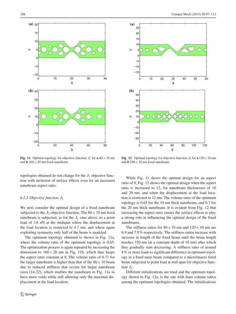
Fig. 11 Optimal topology for objective function J2 for a 80×10 nmand b 160×20 nm fixed nanobeam
topologies obtained do not change for the J1 objective func-tion with inclusion of surface effects even for an increasednanobeam aspect ratio.
6.2.2 Objective function J2
We next consider the optimal design of a fixed nanobeamsubjected to the J2 objective function. The 80×10 nm fixednanobeam is subjected, as for the J1 case above, to a pointload of 3.6 nN at the midspan where the displacement atthe load location is restricted to 4.7 nm, and where againexploiting symmetry only half of the beam is modeled.
The optimum topology obtained is shown in Fig. 11a,where the volume ratio of the optimum topology is 0.65.The optimization process is again repeated by increasing thedimension to 160×20 nm in Fig. 11b, which thus keepsthe aspect ratio constant at 8. The volume ratio of 0.71 forthe larger nanobeam is higher than that of the 80×10 beamdue to reduced stiffness that occurs for larger nanobeamsizes [14,22], which enables the nanobeam in Fig. 11a tohave more voids while still allowing only the maximal dis-placement at the load location.
X
Y
0 10 20 30 40 50 60
−15
−10
−5
0
5
10
15
20
25(a)
X
Y
0 20 40 60 80 100 120
−30
−20
−10
0
10
20
30
40
50(b)
Fig. 12 Optimal topology for objective function J2 for a 120×10 nmand b 240×20 nm fixed nanobeam
While Fig. 11 shows the optimal design for an aspectratio of 8, Fig. 12 shows the optimal design when the aspectratio is increased to 12, for nanobeam thicknesses of 10and 20 nm, and when the displacement at the load loca-tion is restricted to 12 nm. The volume ratio of the optimumtopology is 0.65 for the 10 nm thick nanobeam, and 0.7 forthe 20 nm thick nanobeam. It is evident from Fig. 12 thatincreasing the aspect ratio causes the surface effects to playa strong role in influencing the optimal design of the fixednanobeams.
The stiffness ratios for 80×10 nm and 120×10 nm are6.9 and 7.9% respectively. The stiffness ratios increase withincrease in length of the fixed beam until the beam lengthreaches 320 nm (at a constant depth of 10 nm) after whichthey gradually start decreasing. A stiffness ratio of around8% or more leads to significant difference in optimum topol-ogy in a fixed nano beam compared to a micro/macro fixedbeam subjected to point load at mid span for objective func-tion J2.
Different initializations are tried and the optimum topol-ogy shown in Fig. 12a, is the one with least volume ratiosamong the optimum topologies obtained. The initializations
123
Comput Mech (2015) 56:97–112 109
X
Y
0 10 20 30 40 50 60
−15−10
−505
10152025
(a)
X
Y
0 10 20 30 40 50 60
−15
−10
−5
05
10
15
20
25(b)
X
Y
0 10 20 30 40 50 60
−15−10
−505
10152025
(c)
X
Y
0 10 20 30 40 50 60
−15
−10
−5
05
10
15
20
25(d)
Fig. 13 Initialization a, c and their corressponding Optimal topologiesb, d for objective function J2 for 120×10 nm
and the corresponding optimum topologies are shown inFig. 13.
7 Conclusion
We have presented a coupled XFEM/level set methodologyto perform shape and topology optimization of nanostruc-tureswhile accounting for nanoscale surface effects. The newformulationwas used in conjunctionwith two objective func-tions, those of minimum potential energy and least squareerror in the targeted displacement. While surface effects didnot impact the optimized structure for theminimum potentialenergy objective function, substantial size and aspect ratioeffects were observed for the least square displacement errorobjective function. These arise due to the change in volumeand stiffness ratios. Thus optimum topologies are influencedby the size-dependent stiffening of nanostructures that occurswith decreasing size as a result of the surface effects. Overall,the methodology presented here should enable new insightsand approaches to designing and engineering the behaviorand performance of nanoscale structural elements.
There are many opportunities for future work. For exam-ple, due to the ubiquitous nature of nanobeams in NEMS,work could be done to optimize geometries to produce adesired resonant frequency. Opportunities also exist to pur-sue the optimization of nanobeams where the coupling ofphysics, i.e. electrical and mechanical, are of interest. Workis this respect is already underway.
Acknowledgments Timon Rabczuk and Navid Valizadeh gratefullyacknowledge the financial support of the Framework Programme 7 Ini-tial TrainingNetwork Funding under grant number 289361 “IntegratingNumerical Simulation andGeometricDesignTechnology”.HaroldParkacknowledges the support of the Mechanical Engineering departmentat Boston University. S. S. Nanthakumar gratefully acknowledges thefinancial support of DAAD.
Appendix: Derivation of shape derivative
Firstly, the total potential energy objective function is consid-ered. The objective function and its constraints are as follows,
The material derivative of the Lagrangian is defined as ,
L = J + l(w,Ω) − a(u,w,Ω)
− as(u,w,Ω) − ls(w,Ω). (63)
All the terms that contain w′ in the material derivative ofLagrangian are collected and the sum of these terms is set tozero, to get the weak form of the state equation,
∫
Ω
w′.b dΓ +∫
ΓN
w′.t dΓ =∫
Ω
ε(u) : Cbulk : ε(w′) dΩ
+∫
Γ
Pε(w′)P : τ s dΓ +∫
Γ
(Pε(u)P : Cs : Pε(w′)P) dΓ.
(64)
All the terms that contain u′ in the material derivative ofLagrangian are collected and the sum of these terms is set to
zero, to get the weak form of the adjoint equation,
∫
Ω
u′.b dΓ +∫
ΓN
u′.t dΓ =∫
Ω
ε(u′) : Cbulk : ε(w) dΩ
+∫
Γ
(Pε(u′)P : Cs : Pε(w)P) dΓ. (65)
Considering that ΓN and ΓD are not modified in theoptimization process and assuming that the body forces arezero, the shape derivative of the objective functional can beobtained from Eq. 63,
J ′ =∫
ΓH
G.VndΓ (66)
where,
G = −∫
Γ
ε(u) : Cbulk : ε(w) dΓ
−∫
Ω
κ(Pε(w)P : τ s)
)dΓ
−∫
Γ
κ(Pε(u)P : Cs : Pε(w)P
)dΓ (67)
The G obtained can be considered as the negative of veloc-ity, Vn required in order to optimize the level set function.Therefore,
J ′ = −∫
ΓH
G2dΓ. (68)
From the above equation it is evident that the derivative isnegative (i.e.) it ensures decrease in the objective functionwith iterations.
If the objective function is a least square error comparedto target displacement as shown below,
J (Ω) =⎛
⎜⎝
∫
ΓN
|u − u0|2dΓ
⎞
⎟⎠
12
(69)
J = c0 ·⎛
⎜⎝
∫
ΓN
2|u − u0|u′dΓ +∫
ΓN
(∇(|u − u0|2
)· n
+ κ|u − u0|2⎞
⎟⎠ Vn dΓ. (70)
123
Comput Mech (2015) 56:97–112 111
Substituting in Eq. 63 and collecting terms with u′, the weakform of the adjoint can be obtained as,
c0
∫
ΓN
2|u − u0| u′dΓ =∫
Ω
ε(u′)Cbulkε(w)dΩ
+∫
Γ
(Pε(u′)P : Cs : Pε(w)P)dΓ
(71)
where,
c0 = 1
2
⎛
⎜⎝
∫
ΓN
|u − u0|2dΓ
⎞
⎟⎠
− 12
(72)
References
1. Xia Y, Yang P, Sun Y, Wu Y, Mayers B, Gates B, Yin Y, Kim F,Yan H (2003) One-dimensional nanostructures:synthesis, charac-terization, and applications. Adv Mater 15(5):353–389
2. Lieber CM, Wang ZL (2007) Functional nanowires. MRS Bull32:99–108
3. Haiss W (2001) Surface stress of clean and adsorbate-coveredsolids. Rep Prog Phys 64:591–648
4. Cammarata RC (1994) Surface and interface stress effects in thinfilms. Prog Surf Sci 46(1):1–38
5. Zhou LG, HuangH (2004) Are surfaces elastically softer or stiffer?Appl Phys Lett 84(11):1940–1942
6. Park HS, Cai W, Espinosa HD, Huang H (2009) Mechanics ofcrystalline nanowires. MRS Bull 34(3):178–183
7. Park HS, Gall K, Zimmerman JA (2006) Deformation of FCCnanowires by twinning and slip. J Mech Phys Solids 54(9):1862–1881
8. Park HS, Gall K, Zimmerman JA (2005) Shape memory and pseu-doelasticity in metal nanowires. Phys Rev Lett 95:255504
9. Liang W, Zhou M, Ke F (2005) Shape memory effect in Cunanowires. Nano Lett 5(10):2039–2043
10. Weinberger CR, Cai W (2012) Plasticity of metal nano wires.J Mater Chem 22(8):3277–3292
11. Yvonnet J, QuangHL, HeQC (2008) AnXFEM/level set approachto modelling surface/interface effects and to computing the size-dependent effective properties of nanocomposites. Comput Mech42:119–131
12. Yvonnet J, Mitrushchenkov A, Chambaud G, He GC (2011) Finiteelement model of ionic nanowires with sizedependent mechanicalproperties determined by ab initio calculations. Comput MethodsAppl Mech Eng 200:614–625
13. Gao W, Yu SW, Huang GY (2006) Finite element characteriza-tion of the size-dependent mechanical behaviour in nanosystems.Nanotechnology 17(4):1118–1122
14. Farsad M, Vernerey FJ, Park HS (2010) An extended finite ele-ment/level set method to study surface effects on the mechanicalbehavior and properties of nanomaterials. Int J Numer MethodsEng 84:1466–1489
15. GurtinME,MurdochA (1975)A continuum theory of elasticmate-rial surfaces. Arch Ration Mech Anal 57:291–323
16. Javili A, Steinmann P (2009) A finite element framework for con-tinua with boundary energies. part I: the two dimensional case.Comput Methods Appl Mech Eng 198:2198–2208
17. Javili A, Steinmann P (2010) A finite element framework for con-tinua with boundary energies. part II: the three dimensional case.Comput Methods Appl Mech Eng 199:755–765
18. Park HS, Klein PA, Wagner GJ (2006) A surface cauchy-bornmodel for nanoscale materials. Int J NumerMethods Eng 68:1072–1095
19. Park HS, Klein PA (2007) Surface cauchy-born analysis of surfacestress effects on metallic nanowires. Phys Rev B 75:085408
20. Park HS, Klein PA (2008) A surface cauchy-born model for siliconnanostructures. Comput Methods Appl Mech Eng 197:3249–3260
21. Javili A, McBride A, Steinmann P (2012) Thermomechanics ofsolids with lower-dimensional energetics: on the importance ofsurface, interface, and curve structures at the nanoscale a unifyingreview. Appl Mech Rev 65:010802
22. Park HS, Klein PA (2008) Surface stress effects on the resonantproperties ofmetal nanowires: the importance of finite deformationkinematics and the impact of the residual surface stress. J MechPhys Solids 56:3144–3166
23. Natarajan S, Chakraborty S, Thangavel M, Bordas S, Rabczuk T(2012) Size-dependent free flexural vibration behavior of function-ally graded nanoplates. Comput Mater Sci 65:74–80
24. Yun G, Park HS (2009) Surface stress effects on the bending prop-erties of fcc metal nanowires. Phys Rev B 79:195421
25. He J, Lilley CM (2008) Surface effect on the elastic behavior ofstatic bending nanowires. Nano Lett 8(7):1798–1802
26. Bendsoe MP, Kikuchi N (1988) Generating optimal topologies instructural design using a homogenization method. Comput Meth-ods Appl Mech Eng 71:197–224
27. Allaire G, Jouve F, Toader AM (2004) Structural optimizationusing sensitivity analysis and a level-set method. J Comput Phys194:363–393
28. Luo Z,WangMY,Wang S,Wei P (2008) A level set-based parame-terization method for structural shape and topology optimization.Int J Nume Methods Eng 76(1):1–26
29. Melenk JM, Babuska I (1996) The partition of unity finite ele-mentmethod: basic theory and applications.ComputMethodsApplMech Eng 139(1–4):289–314
30. Osher SJ, Sethian JA (1988) Fronts propagating with curvaturedependent speed: algorithms based on the Hamilton-Jacobi formu-lations. J Comput Phys 79:12–49
31. Sethian JA, Wiegmann A (2000) Structural boundary design vialevel set and immersed interfacemethods. J Comput Phys 163:489–528
32. Osher S, Santosa F (2001) Level-set methods for optimizationproblem involving geometry and constraints: I frequencies of atwo-density inhomogeneous drum. J Comput Phys 171:272–288
33. Wang MY, Wang XM, Guo DM (2003) A level set method forstructural topology optimization.ComputMethodsApplMechEng192:217–224
34. Nanthakumar SS, Lahmer T, Rabczuk T (2014) Detection of mul-tiple flaws in piezoelectric structures using XFEM and level sets.Comput Methods Appl Mech Eng 275:98–112
35. Choi KK, Kim NH (2005) Structural sensitivity analysis and opti-mization. Springer, New York
36. van Dijk NP, Maute K, Langelaar M, Keulen FV (2013) Level-set methods for structural topology optimization: a review. StructMultidiscip Optim 48:437–472
37. Malladi R, Sethian JA, Vemuri BC (1995) Shape modeling withfront propagation: a level set approach. IEEE Trans Pattern AnalMach Intell 17:158–175
38. Stolarska M, Chopp DL, Moes N, Belytschko T (2001) Modelingcrack growth by level sets in the extended finite element method.Int J Numer Methods Eng 51:943–960
123
112 Comput Mech (2015) 56:97–112
39. Sukumar N, Chopp DL, Moes N, Belytschko T (2001) Modelingholes and inclusions by level sets in the extended finite-elementmethod. Comput Methods Appl Mech Eng 190:6183–6200
40. Moes N, Cloirec M, Cartraud P, Remacle JF (2003) A compu-tational approach to handle complex microstructure geometries.Comput Methods Appl Mech Eng 192:3163–3177