SURFACE FINITE ELEMENTS FOR PARABOLIC EQUATIONSmasgat/PAPERS/SurfacePDES/DziEll07... · Surface...

Journal of Computational Mathematics, Vol.25, No.4, 2007, 385–407.

SURFACE FINITE ELEMENTS FOR PARABOLICEQUATIONS *1)

G. Dziuk

(Abteilung fur Angewandte Mathematik, University of Freiburg, Hermann-Herder-Straße 10 D–79104,

Freiburg i. Br., Germany

Email: [email protected])

C. M. Elliott

(Department of Mathematics, University of Sussex, Falmer Brighton BN1 9RF, United Kingdom

Email: [email protected])

Abstract

In this article we define a surface finite element method (SFEM) for the numerical

solution of parabolic partial differential equations on hypersurfaces Γ in Rn+1. The key

idea is based on the approximation of Γ by a polyhedral surface Γh consisting of a union of

simplices (triangles for n = 2, intervals for n = 1) with vertices on Γ. A finite element space

of functions is then defined by taking the continuous functions on Γh which are linear affine

on each simplex of the polygonal surface. We use surface gradients to define weak forms

of elliptic operators and naturally generate weak formulations of elliptic and parabolic

equations on Γ. Our finite element method is applied to weak forms of the equations. The

computation of the mass and element stiffness matrices are simple and straightforward.

We give an example of error bounds in the case of semi-discretization in space for a fourth

order linear problem. Numerical experiments are described for several linear and nonlinear

partial differential equations. In particular the power of the method is demonstrated by

employing it to solve highly nonlinear second and fourth order problems such as surface

Allen-Cahn and Cahn-Hilliard equations and surface level set equations for geodesic mean

curvature flow.

Mathematics subject classification: 65M60, 65M30, 65M12, 65Z05, 58J35, 53A05, 74S05,

80M10, 76M10.

Key words: Surface partial differential equations, Surface finite element method, Geodesic

curvature, Triangulated surface.

1. Introduction

Partial differential equations on surfaces occur in many applications. For example, tradi-

tionally they arise naturally in fluid dynamics and material science and more recently in the

mathematics of images. In this paper we propose a mathematical approach to the formulation

and finite element approximation of parabolic equations on a surface in Rn+1 (n = 1, 2). We

give examples of linear and nonlinear equations. In particular we show how surface level set

and phase field models can be used to compute the motion of curves on surfaces.

* Received September 25, 2006; final revised February 8, 2007; accepted March 3, 2007.1) The work was supported by the Deutsche Forschungsgemeinschaft via DFG-Forschergruppe Nonlinear par-

tial differential equations: Theoretical and numerical analysis and by the UK EPSRC via the Mathematics

Research Network: Computation and Numerical analysis for Multiscale and Multiphysics Modelling. Part of

this work was done during a stay of the first author at the ICM at the University of Warsaw supported by the

Alexander von Humboldt Honorary Fellowship 2005 granted by the Foundation for Polish Science.

386 G. DZIUK AND C. M. ELLIOTT

1.1. The diffusion equation

Conservation on a hypersurface Γ of a scalar u with a diffusive flux −D∇Γw, where D is

the diffusivity tensor and w is a scalar, leads to the diffusion equation

ut −∇Γ · (D∇Γw) = 0 (1.1)

on Γ. Here ∇Γ is the tangential or surface gradient. If ∂Γ is empty then the equation does not

need a boundary condition. Otherwise we can impose Dirichlet or no flux boundary conditions

on ∂Γ. Choosing various constitutive relations to define the relationship between the flux and

u leads to a variety of second and fourth order linear and nonlinear parabolic equations. For

example the constitutive relations w = u and w = −∆Γu lead to linear second and fourth order

diffusion equations.

1.2. The finite element method

In this paper we propose a finite element approximation based on the variational form

∫

Γ

utϕ+

∫

Γ

D∇Γw · ∇Γϕ = 0 (1.2)

where ϕ is an arbitrary test function defined on the surface Γ in R3 with ∂Γ empty. This

provides the basis of our surface finite element method (SFEM) which is applicable to arbitrary

n–dimensional hypersurfaces in Rn+1 (curves in R

2) with or without boundary. Indeed this is

the extension of the method from [10] for the Laplace-Beltrami equation, which was extended

to linear second order diffusion equations on moving surfaces in [12]. We focus our description

on the case n = 2 but observe that the approach is directly applicable to n = 1.

The principal idea is to use a polyhedral approximation of Γ based on a triangulated surface.

It follows that a quite natural local piecewise linear parametrization of the surface is employed

rather than a global one. The finite element space is then the space of continuous piecewise

linear functions on the triangulated surface. The implementation is thus rather similar to that

for solving the diffusion equation on flat stationary domains. For example, for w = u, the

backward Euler time discretization leads to the SFEM scheme

1

τ

(

Mαm+1 −Mαm)

+ Sαm+1 = 0

where M and S are the surface mass and stiffness matrices and αm is the vector of nodal

values for the approximation of u at time tm. Here, τ denotes the time step size. Observe that

this approach to evolutionary surface partial differential equations was used in [11] to evolve a

surface by mean curvature flow. See also [5].

1.3. Level set or implicit surface approach

An alternative approach to our method based on the use of (1.2) is to embed the surface in a

family of level set surfaces [1, 3, 4, 13, 14, 21, 30]. This Eulerian approach can be discretized on

a Cartesian grid in Rn+1 and has the usual advantages and disadvantages of level set methods.

Equations on surfaces also arise in phase field models [7, 19, 25].

Surface Finite Elements for Parabolic Equations 387

1.4. Applications

Models involving partial differential equations on surfaces arise in many areas including ma-

terial science, bio-physics, fluid mechanics and image processing. For example, phase formation

of surface alloying by spinodal decomposition resulting in two dimensional structures has been

modelled by the Cahn-Hilliard equation on surfaces, [8]. See also [26, 27] for studies of the

Allen-Cahn and Cahn-Hilliard equations in the context of phase ordering on surfaces. Other

examples in the physical sciences include diffusion induced grain boundary motion [7, 19, 23]

and the Ginzburg-Landau model for superconductivity [9]. In image processing we mention

geodesic flow of curves on surfaces and active contours for segmentation on surfaces, [22, 24].

1.5. Outline of paper

The layout of the paper is as follows. We begin in Section 2 by defining notation and essential

concepts from elementary differential geometry necessary to describe the problem and numerical

method. Several linear and nonlinear partial differential equations of second and fourth order

are described in Section 3 together with a number of computational results. In Section 4 the

finite element method is defined and some preliminary approximation results are shown. Error

bounds for the semi-discretization in space are proved in Section 5. Implementation issues are

discussed in Section 6.

2. Basic Notation and Surface Derivatives

Let Γ be a compact smooth connected and oriented hypersurface in Rn+1 (n = 1, 2). In

order to formulate the model it is convenient to use a level set description of Γ.

We assume the existence of a smooth level set function d = d(x), x ∈ Rn+1, so that

Γ = {x ∈ N| d(x) = 0} ,

where N is an open subset of Rn+1 in which ∇d 6= 0 and chosen so that

d ∈ C2(N ).

The orientation of Γ is fixed by taking the normal ν to Γ to be in the direction of increasing d.

Hence we define a normal vector field by

ν(x) =∇d(x)

|∇d(x)|.

Throughout this paper we denote by P(x) the projection at x onto the tangent space of Γ with

i, j element

P(x)ij = δij − ν(x)iν(x)j . (2.1)

Observe that a possible choice for d is a signed distance function and in that case |∇d| = 1

on N . For later use we mention that N can be chosen such that for every x ∈ N there exists

a unique a(x) ∈ Γ such that

x = a(x) + d(x)ν(a(x)), (2.2)

where d denotes the signed distance function to Γ.


For any function η defined on an open subset N of Rn+1 containing Γ we define its tangential

gradient on Γ by

∇Γη = ∇η −∇η · ν ν = P∇η,

where, for x and y in Rn+1, x · y denotes the usual scalar product and ∇η denotes the usual

gradient on Rn+1. The tangential gradient ∇Γη only depends on the values of η restricted to Γ

and ∇Γη · ν = 0. The components of the tangential gradient will be denoted by

∇Γη =(

D1η, . . . , Dn+1η)

.

The Laplace-Beltrami operator on Γ is defined as the tangential divergence of the tangential

gradient:

∆Γη = ∇Γ · ∇Γη =

n+1∑

i=1

DiDiη.

Let Γ have a boundary ∂Γ whose intrinsic unit outer normal (conormal), tangential to Γ, is

denoted by µ. Then for i = 1, 2, . . . , n+ 1, the formula for integration on Γ is, see [15],

∫

Γ

Diη = −

∫

Γ

ηHνi +

∫

∂Γ

ηµi, (2.3)

yielding the divergence theorem for ξ = (ξ1, ξ2, . . . , ξn+1),

∫

∂Γ

ξ · µ =

∫

Γ

∇Γ · ξ +

∫

Γ

ξ · νH (2.4)

where H denotes the mean curvature of Γ with respect to ν, which is given by

H = −∇Γ · ν. (2.5)

The orientation is such that for a sphere Γ = {x ∈ Rn+1| |x − x0| = R} and the choice

d(x) = R − |x − x0| the normal is pointing into the ball BR(x0) = {x ∈ Rn+1| |x − x0| < R}

and the mean curvature of Γ is given by H = n/R. Note that H is the sum of the principle

curvatures rather than the arithmetic mean and hence differs from the common definition by a

factor n. The mean curvature vector Hν is invariant with respect to the choice of the sign of d.

Green’s formula on the surface Γ is∫

Γ

∇Γξ · ∇Γη =

∫

∂Γ

ξ∇Γη · µ−

∫

Γ

ξ∆Γη. (2.6)

If Γ is closed then ∂Γ is empty and the boundary terms in equations (2.3),(2.4), and (2.6) do

not appear. For these facts about tangential derivatives we refer to [20], pp. 389-391. Note

that, in general, higher order tangential derivatives do not commute.

We shall use Sobolev spaces on surfaces Γ. For a given surface Γ we define

H1(Γ) = {η ∈ L2(Γ) | ∇Γη ∈ L2(Γ)n+1}

and, if ∂Γ 6= ∅,

H10 (Γ) = {η ∈ H1(Γ) | η = 0 on ∂Γ}.

For smooth enough Γ we analogously define the Sobolev spaces Hk(Γ) for k ∈ N. See [29] for

additional information.


3. Parabolic Equations on Surfaces

3.1. Conservation and diffusion on a surface

Let u = u(x, t) (x ∈ Γ, t ∈ [0, T ]) be the density of a scalar quantity on Γ (for example

mass per unit area if n = 2 or mass per unit length if n = 1). The basic conservation law we

wish to consider can be formulated for an arbitrary portion M of Γ using a surface flux q. The

law is that, for every M,d

dt

∫

M

u = −

∫

∂M

q · µ, (3.1)

where ∂M is the boundary of M (a curve if n = 2 and the end points of a curve if n = 1) and

µ is the conormal on ∂M. Thus µ is the unit normal to ∂M pointing out of M and tangential

to Γ. Observe that components of q normal to M do not contribute to the flux, so, without

loss of generality, we assume that q is a tangent vector.

Using the divergence theorem (2.4) and the fact that q is a tangential vector we obtain∫

∂M

q · µ =

∫

M

∇Γ · q +

∫

M

q · νH =

∫

M

∇Γ · q,

so that∫

M

(ut + ∇Γ · q) = 0,

which implies the pointwise conservation law

ut + ∇Γ · q = 0 on Γ. (3.2)

We take q to be the diffusive flux

q = −D∇Γw, (3.3)

where D ≥ 0 is a symmetric mobility tensor with the property that it maps the tangent space

into itself at every point of Γ, i.e.,

Dν⊥ · ν = 0 (3.4)

for every tangent vector ν⊥. This leads to the equation

ut −∇Γ · (D∇Γw) = 0 on Γ. (3.5)

Since ∂Γ = ∅, i.e., the surface has no boundary, there is no need for boundary conditions. For

example, this would be the case if Γ is the bounding surface of a domain.

Remark 3.1. If ∂Γ is non-empty then we may impose the homogeneous Dirichlet boundary

condition

u = 0 on ∂Γ, (3.6)

or impose the no flux condition

D∇Γw · µ = 0 on ∂Γ. (3.7)

The variational form (1.2) then is an easy consequence of (1.1). We multiply equation (1.1) by

an arbitrary test function ϕ ∈ H1(Γ) and integrate over Γ. We then obtain using (2.4):∫

Γ

utϕ+

∫

Γ

D∇Γw · ∇Γϕ = 0. (3.8)

Here and in all subsequent equations we have to impose an initial condition u(·, 0) = u0. In the

following we will not mention this condition when it is obviously required.


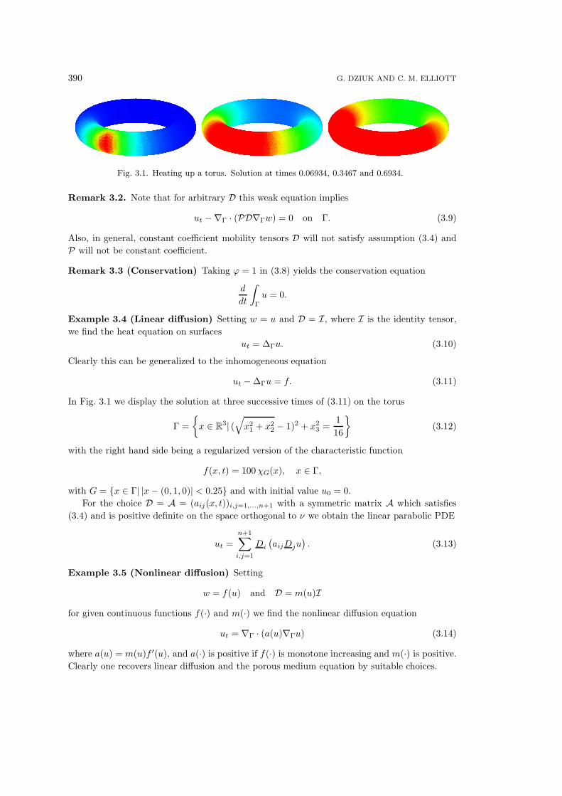
Fig. 3.1. Heating up a torus. Solution at times 0.06934, 0.3467 and 0.6934.

Remark 3.2. Note that for arbitrary D this weak equation implies

ut −∇Γ · (PD∇Γw) = 0 on Γ. (3.9)

Also, in general, constant coefficient mobility tensors D will not satisfy assumption (3.4) and

P will not be constant coefficient.

Remark 3.3 (Conservation) Taking ϕ = 1 in (3.8) yields the conservation equation

d

dt

∫

Γ

u = 0.

Example 3.4 (Linear diffusion) Setting w = u and D = I, where I is the identity tensor,

we find the heat equation on surfaces

ut = ∆Γu. (3.10)

Clearly this can be generalized to the inhomogeneous equation

ut − ∆Γu = f. (3.11)

In Fig. 3.1 we display the solution at three successive times of (3.11) on the torus

Γ =

{

x ∈ R3| (√

x21 + x2

2 − 1)2 + x23 =

1

16

}

(3.12)

with the right hand side being a regularized version of the characteristic function

f(x, t) = 100χG(x), x ∈ Γ,

with G = {x ∈ Γ| |x− (0, 1, 0)| < 0.25} and with initial value u0 = 0.

For the choice D = A = (aij(x, t))i,j=1,...,n+1 with a symmetric matrix A which satisfies

(3.4) and is positive definite on the space orthogonal to ν we obtain the linear parabolic PDE

ut =

n+1∑

i,j=1

Di

(

aijDju)

. (3.13)

Example 3.5 (Nonlinear diffusion) Setting

w = f(u) and D = m(u)I

for given continuous functions f(·) and m(·) we find the nonlinear diffusion equation

ut = ∇Γ · (a(u)∇Γu) (3.14)

where a(u) = m(u)f ′(u), and a(·) is positive if f(·) is monotone increasing and m(·) is positive.

Clearly one recovers linear diffusion and the porous medium equation by suitable choices.


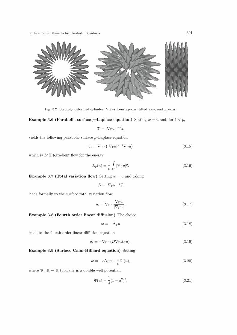
Fig. 3.2. Strongly deformed cylinder: Views from x3-axis, tilted axis, and x1-axis.

Example 3.6 (Parabolic surface p–Laplace equation) Setting w = u and, for 1 < p,

D = |∇Γu|p−2I

yields the following parabolic surface p–Laplace equation

ut = ∇Γ ·(

|∇Γu|p−2∇Γu

)

(3.15)

which is L2(Γ)-gradient flow for the energy

Ep(u) =1

p

∫

Γ

|∇Γu|p. (3.16)

Example 3.7 (Total variation flow) Setting w = u and taking

D = |∇Γu|−1I

leads formally to the surface total variation flow

ut = ∇Γ ·∇Γu

|∇Γu|. (3.17)

Example 3.8 (Fourth order linear diffusion) The choice

w = −∆Γu (3.18)

leads to the fourth order linear diffusion equation

ut = −∇Γ · (D∇Γ∆Γu) . (3.19)

Example 3.9 (Surface Cahn-Hilliard equation) Setting

w = −ǫ∆Γu+1

ǫΨ′(u), (3.20)

where Ψ : R → R typically is a double well potential,

Ψ(u) =1

4(1 − u2)2, (3.21)


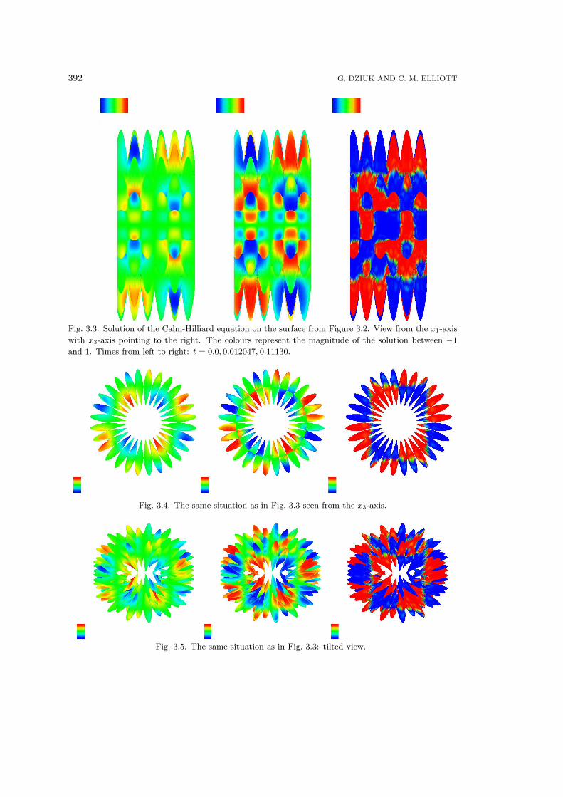
Fig. 3.3. Solution of the Cahn-Hilliard equation on the surface from Figure 3.2. View from the x1-axis

with x3-axis pointing to the right. The colours represent the magnitude of the solution between −1

and 1. Times from left to right: t = 0.0, 0.012047, 0.11130.

Fig. 3.4. The same situation as in Fig. 3.3 seen from the x3-axis.

Fig. 3.5. The same situation as in Fig. 3.3: tilted view.


leads to the fourth order Cahn-Hilliard equation

ut = −∇Γ ·

(

D∇Γ(ǫ∆Γu−1

ǫΨ′(u))

)

. (3.22)

Using second order splitting as introduced in [17] we formulate the problem as a system of

second order equations in space. We solved the Cahn-Hilliard equation for D = I on a strongly

deformed surface (see Fig. 3.2). The topology of the surface is cylindrical: Γ = F (Γ0), where

F (x1, x2, x3) = f(x1, x2, x3)(x1, x2, 0) + (0, 0, x3)

with f(x) = 1+0.5 sin (14ϕ) sin (15x3) and ϕ is the polar angle in the x1, x2-plane. As reference

surface we have chosen the cylinder Γ0 = {x ∈ R3|x2

1 + x22 < 1, 0 < x3 < 1.2}. As initial value

we have taken

u0(x) = sin (4x1) sin (3x2) sin (5x3).

The grid contained N = 24960 nodes. We have used ε = 0.01. Colour maps of the solution are

depicted in Figs. 3.3, 3.4 and 3.5.

3.2. Equations in non-conservation form

Here we formulate several time dependent equations on surfaces which are not in conserva-

tion form.

Example 3.10 (Surface Allen-Cahn equation) Consideration of the L2(Γ)-gradient flow

for the gradient energy functional

E(v) =

∫

Γ

(

ǫ

2|∇Γv|

2 +Ψ(v)

ǫ

)

, (3.23)

(ǫ > 0) leads to

ǫut = ǫ∆Γu−1

ǫΨ′(u). (3.24)

Here the potential (3.21) gives the classical Allen-Cahn equation on a surface Γ.

In Fig. 3.6 we show results of the numerical solution of the surface Allen-Cahn equation on

the torus (3.12) with initial data

u0(x) = sin (3πx3) cos (3ϕ),

where ϕ denotes the polar angle in the x1, x2-plane. We observe the rapid evolution to a

checkerboard pattern on the torus (first row). After some time this pattern is dissolved and the

solution evolves to an interesting stationary solution (second row). It is interesting to observe

that the red and blue regions are connected, so that there is just one diffuse interface which

approximates a curve of zero geodesic curvature.

In Fig. 3.7 we show the typical decomposition effect of the Allen-Cahn equation on a de-

formed cylinder. Here the initial value u0 was chosen to be a random distribution of matter on

the surface.

Example 3.11 (Level set geodesic mean curvature flow) We formulate the level set equa-

tion

ut = |∇Γu| ∇Γ ·∇Γu

|∇Γu|. (3.25)


Fig. 3.6. Solution of the surface Allen-Cahn equation on a torus.

Fig. 3.7. Solution of the Allen-Cahn equation on a deformed cylinder (surface, initial distribution,

distribution after some time).

For example, we have in mind the evolution, on the fixed surface Γ in R3, of a closed curve C(t)

which is evolving in the “intrinsic” normal direction νg with a velocity Vg given by minus its

geodesic curvature κg. The curve C(t) is given by the zero level set on Γ of u(·, t) and

νg =∇Γu

|∇Γu|, κg = ∇Γ ·

∇Γu

|∇Γu|, Vg = −

ut

|∇Γu|.

Fig. 3.8 shows how circles on a dumbbell shaped surface move under geodesic mean curvature

flow. The surface Γ is given as Γ = F (S2) where F (x) = (x1, η(x)x2, η(x)x3) with

η(x) =√

1 − x21

√

1 − 0.8(1 − x21)

2/√

x22 + x2

3

for x ∈ S2. The initial function is u0(x) = x1 − 0.25. In Fig. 3.8 we display all the level lines

{x ∈ Γ|u(x, t) = c} for c between −1.05 and 1.25 with intervals of 0.2.

We observe that circles shrink and either move to the center of the dumbbell’s neck or shrink

to round points at the extreme ends of the dumbbell. Each of these possibilities is displayed in

Fig. 3.9 for a single circle.

Finally in Fig. 3.10 we show the evolution of many level sets on the sphere. We see topology

change of the level sets. In this computation we use the initial value

u0(x) = sin(5π(x1 − 0.25)) sin (3π(x3 + 0.25)).

In all these computations of geodesic curve shortening flow we regularized the equations by

replacing |∇Γu| by√

ε2 + |∇Γu|2, and we have taken the parameter ε proportional to the grid

size h.


Fig. 3.8. Geodesic curve shortening flow on a dumbbell.

Fig. 3.9. Geodesic curve shortening flow for two circles on a dumbbell.

Fig. 3.10. Level set mean curvature flow on the sphere.

Example 3.12 (Level Set Surface Active Contours) We formulate the level set equation

ut = |∇Γu|∇Γ ·

(

f∇Γu

|∇Γu|

)

(3.26)

where

f =1

1 + |∇ΓIσ|2. (3.27)

In (3.27), Iσ is a smoothed image which is essentially a characteristic function with sharp edges.

The evolution of the zero level set curve C(t) is designed to detect the edge.

Example 3.13 (Anisotropic geodesic level set mean curvature flow) We formulate the

level set equation for anisotropic mean curvature flow on the given surface Γ as

µ(∇Γu)ut = |∇Γu|∇Γ ·Dγ(∇Γu), (3.28)

where γ : Rn+1 \ {0} → (0,∞), γ(0) = 0, is an anisotropy function, smooth and positively ho-

mogeneous of degree one. Here Dγ denotes the gradient of γ. µ is a positive and 0-homogeneous

function.

Example 3.14 (Level set geodesic surface diffusion) We formulate the level set equation

ut = ∇Γ · (|∇Γu|(I − νg ⊗ νg)∇Γw), (3.29)

w = ∇Γ ·∇Γu

|∇Γu|. (3.30)

For example, we have in mind the evolution, on the fixed surface Γ in R3, of a closed curve C(t)

which is evolving in the “intrinsic” normal direction νg with a velocity V given by the geodesic

Laplacian of the geodesic curvature κg. The curve C(t) is given by the zero level set on Γ of

u(·, t).


Example 3.15 (Level set geodesic Willmore flow) We formulate the level set equation

ut = −|∇Γu|∇Γ ·

(

1

|∇Γu|(I − νg ⊗ νg)∇Γw

)

+1

2|∇Γu|∇Γ ·

(

w2

|∇Γu|2∇Γu

|∇Γu|

)

,(3.31)

w = −|∇Γu| ∇Γ ·∇Γu

|∇Γu|. (3.32)

Here the zero level set of u is the curve C(t) constrained to lie on Γ which evolves according to

L2 gradient flow for the energy

EC =1

2

∫

C

κ2g. (3.33)

4. Finite Element Approximation

4.1. Finite elements on surfaces

The smooth surface Γ (∂Γ = ∅) is approximated by a Lipschitz continuous surface Γh ⊂ N

(∂Γh = ∅). In particular for n = 2, Γh = ∪e∈The is a triangulated (and hence polyhedral)

surface consisting of triangles e in Th with maximum diameter being denoted by h and inner

radius bounded below by ch with some c > 0. The vertices {Xj}Nj=1 of the triangles are taken

to sit on Γ so that Γh is an interpolation. Each edge of a triangle e1 ∈ Th is an edge of another

triangle e2 ∈ Th. Note that by (2.2) for every triangle e ⊂ Γh there is a unique curved triangle

T = a(e) ⊂ Γ. In order to avoid a global double covering (see [12]) we assume that,

for each point a ∈ Γ there is at most one point x ∈ Γh with a = a(x). (4.1)

This implies that there is a bijective correspondence between the triangles on Γh and the induced

curvilinear triangles on Γ.

For any continuous function η defined on the discrete surface Γh we may define an extension

or lift onto Γ by

ηl(a) = η(x(a)), a ∈ Γ, (4.2)

where by (2.2) and our assumptions, x(a) is defined as the unique solution of

x = a+ d(x)ν(a). (4.3)

Furthermore we understand by ηl(x) the constant extension from Γ in the normal direction

ν(a). We denote by νh the normal to Γh which is constant on each element e. An application

of the chain rule for differentiation gives

∇Γhη = Ph(I − dH)∇Γη

l(a(x)) (4.4)

where Ph is the discrete projection

Ph,ij = δij − νh,iνh,j

and H is the matrix of second derivatives of the distance function d with i, j element

Hi,j = dxixj.

We have a finite element space

Sh ={

φ ∈ C0(Γh)|φ|e is linear affine for each e ∈ Th

}

= span{χj | j = 1, . . . , N}.


By χj we denote the common nodal basis function from Sh which is 1 at the node Xj and zero

at all other nodes.

It is convenient to introduce

Slh =

{

ηl ∈ C0(Γ)| ηl(a) = η(x(a)), η ∈ Sh and x(a) given by (4.3)}

.

In the error analysis of the finite element scheme we shall need the following technical lemmas

[10].

Lemma 4.1. Assume Γ and Γh are as above and let d denote the oriented distance function

of Γ. Then

‖d‖L∞(Γh) ≤ ch2. (4.5)

Let δh be the quotient between the smooth and discrete surface measures dA on Γ and dAh on

Γh so that δhdAh = dA, and let

Rh =1

δhP(I − dH)Ph(I − dH).

Then we have the following estimates

supΓh

|1 − δh| ≤ ch2, (4.6)

supΓh

|(I −Rh)P| ≤ ch2. (4.7)

Lemma 4.2. Let η : Γh → R with lift ηl : Γ → R. Then for the planar and curved triangles

e ⊂ Γh and T ⊂ Γ the following estimates hold. There is a constant c > 0 independent of h

such that

1

c‖η‖L2(e) ≤ ‖ηl‖L2(T ) ≤ c‖η‖L2(e), (4.8)

1

c‖∇Γh

η‖L2(e) ≤ ‖∇Γηl‖L2(T ) ≤ c‖∇Γh

η‖L2(e), (4.9)

‖∇2Γhη‖L2(e) ≤ c‖∇2

Γηl‖L2(T ) + ch‖∇Γη

l‖L2(T ). (4.10)

In the above we employ the convention that the L2 norm of a vector or matrix is simply the

L2 norm of the l2 norm of the components. We denote by ∇2Γη the matrix of second tangential

derivatives.

It is convenient to introduce a piecewise linear interpolant which is constructed in an obvious

way. Observing that the pointwise linear interpolation Ihη ∈ Sh is well defined for η belonging

to H2(Γ), Ihη is defined by lifting Ihη onto Γ according to (4.2), so that Ihη = (Ihη)l. The

following interpolation results hold, [10].

Lemma 4.3. For given η ∈ H2(Γ) there exists a unique Ihη ∈ Slh such that

‖η − Ihη‖L2(Γ) + h‖∇Γ(η − Ihη)‖L2(Γ) ≤ ch2(

‖∇2Γη‖L2(Γ) + h‖∇Γη‖L2(Γ)

)

. (4.11)

4.2. Semi-discrete approximation

Our SFEM, based on the finite element spaces introduced in this section, is applicable to

all the partial differential equations described in Section 3. Here we give some representative

examples. They show that solving partial differential equations on surfaces in Rn+1 is analogous

to solving equations on domains in Rn. The fourth order problems considered here are treated

by the second order splitting approach of [17].


4.2.1. Conservation and diffusion

We begin by describing the semi-discretization of (3.8) in space. Let (U(·, t),W (·, t)) ∈ Sh ×Sh

be such that∫

Γh

Utφ+

∫

Γh

D−l∇ΓhW · ∇Γh

φ = 0 ∀φ ∈ Sh. (4.12)

Setting

U(·, t) =

N∑

j=1

αj(t)χj(·), W (·, t) =

N∑

j=1

βj(t)χj(·)

we find that, ∀φ ∈ Sh,

∫

Γh

N∑

j=1

αj,tχjφ+

∫

Γh

D−l

N∑

j=1

βj(t)∇Γhχj · ∇Γh

φ = 0

and taking φ = χk, k = 1, . . . , N we obtain

Mα+ Sβ = 0 (4.13)

where

Mjk =

∫

Γh

χjχk , Sjk =

∫

Γh

D−l∇Γhχj∇Γh

χk.

Here D−l is such that its lift is the diffusivity D so that(

D−l)l

= D.

Example 4.4 (Linear diffusion) In this case W=U so that the problem becomes: Find

U(·, t) ∈ Sh such that∫

Γh

Utφ+

∫

Γh

D−l∇ΓhU · ∇Γh

φ = 0 ∀φ ∈ Sh (4.14)

yielding the time dependent ordinary differential equations

Mα+ Sα = 0. (4.15)

Example 4.5 (Fourth order linear diffusion) In this case we employ the following finite

element approximation of (3.18)∫

Γh

Wφ−

∫

Γh

∇ΓhU · ∇Γh

φ = 0 ∀φ ∈ Sh (4.16)

which yields Mβ − S0α = 0, where

S0jk =

∫

Γh

∇Γhχj∇Γh

χk.

Substituting into (4.13) yields

Mα+ SM−1S0α = 0. (4.17)

Example 4.6 (Surface Cahn Hilliard equation) Find (U(·, t),W (·, t)) ∈ Sh×Sh such that∫

Γh

Utφ+

∫

Γh

D−l∇ΓhW · ∇Γh

φ = 0 ∀φ ∈ Sh, (4.18)

∫

Γh

ǫ∇ΓhU · ∇Γh

φ+IhΨ′(U)

ǫφ =

∫

Γh

Wφ ∀φ ∈ Sh. (4.19)


Note the use of IhΨ′(U). The discrete equations become

Mα+ Sβ = 0, Mβ − ǫS0α−1

ǫMΨ′(α) = 0

and eliminating β we obtain

Mα+ ǫSM−1S0α+1

ǫSΨ′(α) = 0. (4.20)

Here we use the notation that (Ψ′(α))j = Ψ′(αj).

4.2.2. Equations in non-conservation form

Example 4.7 (Surface Allen-Cahn equation) The approximate problem is to find U(·, t) ∈

Sh such that

ǫ

∫

Γh

Utφ+

∫

Γh

(

ǫ∇ΓhU · ∇Γh

φ+1

ǫIhΨ′(U)φ

)

= 0 ∀φ ∈ Sh, (4.21)

which may be rewritten in matrix form as

ǫMα+ ǫS0α+1

ǫMΨ′(α) = 0. (4.22)

Example 4.8 (Level set geodesic mean curvature flow) The semi-discrete finite element

approximation is: Find U(·, t) ∈ Sh such that∫

Γh

Ut

|∇ΓhU |ǫ

φ+

∫

Γh

∇ΓhU

|∇ΓhU |ǫ

· ∇Γhφ = 0 ∀φ ∈ Sh. (4.23)

Here we have introduced the following regularized l2 norm |p|ǫ =√

|p|2 + ǫ2 in order to avoid

dividing by zero when ∇ΓhU = 0. It follows that the discrete equations may be written as

MU α+ SUα = 0 (4.24)

where the weighted mass and stiffness matrices are

(MU )jk =

∫

Γh

χjχk

|∇ΓhU |ǫ

, (SU )jk =

∫

Γh

∇Γhχj∇Γh

χk

|∇ΓhU |ǫ

.

Example 4.9 (Level set geodesic surface diffusion) Find (U(·, t),W (·, t)) ∈ Sh×Sh such

that∫

Γh

Utφ+

∫

Γh

|∇ΓhU |Ph

g ∇ΓhW · ∇Γh

φ = 0 ∀φ ∈ Sh, (4.25)

∫

Γh

Wφ+

∫

Γh

∇ΓhU

|∇ΓU |ǫ· ∇Γh

φ = 0 ∀φ ∈ Sh. (4.26)

Here we have used the notation

νhg =

∇ΓhU

|∇ΓhU |ǫ

, Phg = I − νh

g ⊗ νhg .

The discrete equations become

Mα+ Shg β = 0, Mβ − SUα = 0,

and eliminating β we obtain

Mα+ Shg M

−1SUα = 0, (4.27)

where

(Shg )jk =

∫

Γh

|∇ΓhU |Ph

g ∇Γhχj∇Γh

χk.


5. Error Bounds

In this section we will prove convergence results for the parabolic plate equation on a surface

Γ. We do this in order to give a nontrivial example for our approximation methods. Several of

the equations discussed in the previous sections can be treated along the lines of the convergence

proof for the parabolic plate equation on a surface. In order to simplify the presentation we

treat the case D = I only.

5.1. Linear Diffusion

Lemma 5.1 (Stability) Let U , W be a solution of the semi-discrete scheme as in Example

3.8 with initial value U(·, 0) = U0 and U l, W l its lift according to (4.2). Then the following

stability estimates hold:

sup(0,T )

‖U l‖2L2(Γ) +

∫ T

0

‖W l‖2L2(Γ) ≤ c‖U l

0‖2L2(Γ), (5.1)

∫ T

0

‖U lt‖

2L2(Γ) + sup

(0,T )

‖W l‖2L2(Γ) ≤ c‖W l(·, 0)‖2

L2(Γ), (5.2)

sup(0,T )

‖∇ΓUl‖2

L2(Γ) +

∫ T

0

‖∇ΓWl‖2

L2(Γ) ≤ c(‖U l0‖

2L2(Γ) + ‖W l(·, 0)‖2

L2(Γ)). (5.3)

Proof. If we test the diffusion equation (4.12) with φ = Ut and take the time derivative

of the equation (4.16) and then test that equation with φ = W and take the sum of the two

resulting equations we get∫

Γh

U2t +

1

2

d

dt

∫

Γh

W 2 = 0,

which leads to the estimate (5.2).

Choosing φ = U in (4.12), φ = W in (4.16) and taking the sum leads to

1

2

d

dt

∫

Γh

U2 +

∫

Γh

W 2 = 0

and this gives the estimate (5.1).

The estimate (5.3) follows by taking φ = U in (4.16) with the use of the previous estimates.

Similarly the choice φ = W in (4.12) gives the estimate for the gradient of W .

We now can prove a convergence result for piecewise linear finite elements on two dimensional

surfaces. Note that as discrete initial value we take a realistic function which can be computed.

Theorem 5.2 (Convergence) Let u,w = −∆Γu be a sufficiently smooth solution of

ut + ∆2Γu = 0, u(·, 0) = u0 on Γ

on the sufficiently smooth closed surface Γ and let U,W be the discrete solution according to

(4.12) and (4.16). As initial value U0 we take the discrete Ritz projection of the continuous

initial value u0 defined by

∫

Γh

∇ΓhU0 · ∇Γh

φ =

∫

Γh

∇Γhu−l

0 · ∇Γhφ ∀φ ∈ Sh (5.4)


and∫

ΓhU0 = 0. With the lifts U l of U and W l of W we then have the error estimates

supt∈(0,T )

‖u(·, t) − U l(·, t)‖L2(Γ) + h supt∈(0,T )

‖∇Γ(u(·, t) − U l(·, t))‖L2(Γ) ≤ C1h2, (5.5)

and

(

∫ T

0

‖w(·, t) −W l(·, t)‖2L2(Γ) dt

)1

2

+ h

(

∫ T

0

‖∇Γ(w(·, t) −W l(·, t))‖2L2(Γ) dt

)1

2

≤ C2h2,

(5.6)

where

C1 = c( supt∈(0,T )

‖u(·, t)‖H4(Γ) +

(

∫ T

0

‖ut(·, t)‖2H2(Γ)dt

)1

2

+ ‖u0‖H4(Γ)),

C2 = c(

(

∫ T

0

‖u(·, t)‖2H4(Γ)

)1

2

+

(

∫ T

0

‖ut(·, t)‖2H2(Γ) dt

)1

2

+ ‖u0‖H4(Γ)).

Proof. In order to make the proof clearer we only treat the case D = I here. The proof is

easily extended to the general case. The error bounds follow the classic Galerkin error analysis

for parabolic equations [28] and rely on a suitable form of the error equation. In order to

compare discrete and continuous solution both should be defined on the same surface which we

take to be the continuous surface Γ. The continuous equations read

∫

Γ

utϕ+

∫

Γ

∇Γw · ∇Γϕ = 0,

∫

Γ

wψ −

∫

Γ

∇Γu · ∇Γψ = 0 (5.7)

for all ϕ, ψ ∈ H1(Γ), and the discrete equations are given by

∫

Γh

Utφ+

∫

Γh

∇ΓhW · ∇Γh

φ = 0,

∫

Γh

Wψ −

∫

Γh

∇ΓhU · ∇Γh

ψ = 0 (5.8)

for all φ, ψ ∈ Sh. We lift the discrete equations to the continuous surface as it was described in

(4.2). We define U l,W l and φl, ψl by

U(x, t) = U l(a(x), t), W (x, t) = W l(a(x), t),

φ(x) = φl(a(x)), ψ(x) = ψl(a(x))

for points x ∈ Γh. For better understanding of the following, we introduce the notation

uh(x, t) = U l(x, t), wh(x, t) = W l(x, t), x ∈ Γ.

We recall the abbreviation (see Lemma 4.1)

Rh(x) =1

δh(x)P(x)(I − d(x)H(x))Ph(x)(I − d(x)H(x)), x ∈ Γh

together with its lifted version Rlh(a(x)) = Rh(x), x ∈ Γh. Thus (5.8) leads to

∫

Γ

uh,tϕh

1

δlh

+

∫

Γ

Rlh∇Γwh · ∇Γϕh = 0,

∫

Γ

whψh

1

δlh

−

∫

Γ

Rlh∇Γuh · ∇Γψh = 0 (5.9)


for all ϕh, ψh ∈ Slh. We take the differences of the equations (5.7) at ϕh, ψh and (5.9).

The error relation between continuous and lifted discrete solution then is given by

∫

Γ

(ut −1

δlh

uh,t)ϕh +

∫

Γ

(

∇Γw −Rlh∇Γwh

)

· ∇Γϕh = 0, (5.10a)

∫

Γ

(w −1

δlh

wh)ψh −

∫

Γ

(

∇Γu−Rlh∇Γuh

)

· ∇Γψh = 0 (5.10b)

for all ϕh, ψh ∈ Slh, and with the use of the estimates from Lemma 4.1 we obtain

∫

Γ

(u − uh)tϕh +

∫

Γ

∇Γ(w − wh) · ∇Γϕh ≤ ch2

∫

Γ

(|∇Γwh||∇Γϕh| + |uh,t||ϕh|), (5.11a)

∫

Γ

(w − wh)ψh −

∫

Γ

∇Γ(u− uh) · ∇Γψh ≤ ch2

∫

Γ

(|∇Γuh||∇Γψh| + |wh||ψh|) (5.11b)

for all ϕh, ψh ∈ Slh.

We define the Ritz-Galerkin projection vh of a function v as the unique solution vh ∈ Slh

with∫

Γvh = 0 of

∫

Γ

∇Γvh · ∇Γϕh =

∫

Γ

∇Γv · ∇Γϕh ∀ϕh ∈ Slh. (5.12)

It is easily shown, with the help of Lemma 4.3, that for a sufficiently smooth function v one

has the estimates

‖v − vh‖L2(Γ) + h‖∇Γ(v − vh)‖L2(Γ) ≤ ch2‖v‖H2(Γ) (5.13)

and similar estimates for the time derivative of v if vt ∈ H2(Γ).

We now use ϕh = uh − uh and ψh = wh − wh as test functions in (5.11), take the sum of

the two resulting equations, and arrive at

1

2

d

dt‖uh − uh‖

2L2(Γ) + ‖wh − wh‖

2L2(Γ)

≤ ‖uh,t − ut‖L2(Γ)‖uh − uh‖L2(Γ) + ‖wh − w‖L2(Γ)‖wh − wh‖L2(Γ)

+ch2(

‖∇Γwh‖L2(Γ)‖∇Γ(uh − uh)‖L2(Γ) + ‖uh,t‖L2(Γ)‖uh − uh‖L2(Γ)

)

+ch2(

‖∇Γuh‖L2(Γ)‖∇Γ(wh − wh)‖L2(Γ) + ‖wh‖L2(Γ)‖wh − wh‖L2(Γ)

)

≤ ε‖uh − uh‖2L2(Γ) +

1

2‖wh − wh‖

2L2(Γ)

+cεh4(

‖∇Γuh‖2L2(Γ) + ‖∇Γwh‖

2L2(Γ) + ‖uh,t‖

2L2(Γ) + ‖wh‖

2L2(Γ) + ‖ut‖

2H2(Γ)

+‖w‖2H2(Γ)

)

+ ε‖∇Γ(uh − uh)‖2L2(Γ) + ε‖∇Γ(wh − wh)‖2

L2(Γ). (5.14)

Here ε is a positive number which will be chosen later. The last two terms on the right hand side

of this inequality are treated as follows. In (5.10) we choose ϕh = wh −wh and ψh = uh,t −uh,t

as test functions and subtract the resulting equations. Thus

∫

Γ

(∇Γwh −Rlh∇Γwh) · ∇Γ(wh − wh) +

∫

Γ

(∇Γuh −Rlh∇Γuh) · ∇Γ(uh,t − uh,t)

= −

∫

Γ

(

(ut −1

δlh

uh,t)(wh − wh) − (w −1

δlh

wh)(uh,t − uh,t)

)

. (5.15)


We estimate the terms in this equation separately. For the first term on the left hand side we

have with Lemma 4.1∫

Γ

(∇Γwh −Rlh∇Γwh) · ∇Γ(wh − wh)

≥

∫

Γ

|∇Γ(wh − wh)|2 − ch2

∫

Γ

|∇Γwh||∇Γ(wh − wh)|

≥1

2

∫

Γ

|∇Γ(wh − wh)|2 − ch4

∫

Γ

|∇Γwh|2. (5.16)

The second term on the left hand side of (5.15) is treated as follows:

∫

Γ

(∇Γuh −Rlh∇Γuh) · ∇Γ(uh,t − uh,t)

≥1

2

d

dt

∫

Γ

Rlh∇Γ(uh − uh) · ∇Γ(uh − uh) +

d

dt

∫

Γ

(I −Rlh)∇Γuh · ∇Γ(uh − uh)

−ε

∫

Γ

|∇Γ(uh − uh)|2 − cεh4

∫

Γ

|∇Γuh,t|2. (5.17)

Here we have used the symmetry of the matrix PRlhP .

And the right hand side of (5.15) is rewritten as

∫

Γ

(

(ut −1

δlh

uh,t)(wh − wh) − (w −1

δlh

wh)(uh,t − uh,t)

)

=d

dt

∫

Γ

(u− uh)(1

δlh

wh − w) −

∫

Γ

(u− uh)(1

δlh

wh,t − wt)

+

∫

Γ

(ut − uh,t)(w − wh) +

∫

Γ

(utwh − uh,twh)(1 −1

δlh

)

≥d

dt

∫

Γ

(u− uh)(1

δlh

wh − w) − ε

∫

Γ

(uh − uh)2 − ε

∫

Γ

(wh − wh)2

−cεh4(‖u‖2

H2(Γ) + ‖ut‖2H2(Γ) + ‖w‖2

H2(Γ) + ‖wt‖2H2(Γ)). (5.18)

We now collect the estimates (5.16), (5.17) and (5.18), integrate with respect to time. For

h ≤ h0 this gives the estimate

‖∇Γ(uh − uh)‖2L2(Γ) +

∫ t

0

‖∇Γ(wh − wh)‖2L2(Γ) dt

≤ ε‖uh − uh‖2L2(Γ) + ε

∫ t

0

‖uh − uh‖2H1(Γ) dt+ ε

∫ t

0

‖wh − wh‖2L2(Γ) dt

+cεh4

(

‖u‖2H2(Γ) + ‖w‖2

H2(Γ) +

∫ t

0

‖u‖2H2(Γ) + ‖w‖2

H2(Γ) dt

)

+A0,h. (5.19)

By A0,h we denote the contribution of the initial values

A0.h =1

2

∫

Γ

Rlh∇Γ(uh(·, 0) − uh(·, 0)) · ∇Γ(uh(·, 0) − uh(·, 0))

+

∫

Γ

(I −Rlh)∇Γuh(·, 0) · ∇Γ(uh(·, 0) − uh(·, 0))

+

∫

Γ

(u0 − uh(·, 0))(1

δlh

wh(·, 0) − w(·, 0)).


Our choice of uh0 = U l0 (see (5.4)) leads to

‖∇Γ(uh(·, 0) − uh0)‖L2(Γ) ≤ ch3‖u0‖H2(Γ), (5.20)

‖uh(·, 0) − uh0‖L2(Γ) ≤ ch2‖u0‖H2(Γ). (5.21)

This estimate is left to the reader. It is an easy consequence of the definition of the discrete

initial value, the geometric estimates from Lemma 4.1 and the assumptions on the mean values

of uh(·, 0) and uh0.

Altogether we arrive at the following estimate for the gradient terms:

‖∇Γ(uh − uh)‖2L2(Γ) +

∫ t

0

‖∇Γ(wh − wh)‖2L2(Γ) dt

≤ ε‖uh − uh‖2L2(Γ) + ε

∫ t

0


∫ t

0


+cεh4

(

‖u‖2H2(Γ) + ‖w‖2

H2(Γ) +

∫ t

0

‖u‖2H2(Γ) + ‖w‖2

H2(Γ) dt+ ‖u0‖2H2(Γ)

)

. (5.22)

We now integrate estimate (5.14) with respect to time and get

‖uh − uh‖2L2(Γ) +

∫ t

0


≤ ε

∫ t

0


∫ t

0

‖∇Γ(wh − wh)‖2L2(Γ) dt+ cεh

4

(∫ t

0

‖∇Γuh‖2L2(Γ)

+‖wh‖2H1(Γ) + ‖uh,t‖

2L2(Γ) + ‖ut‖

2H2(Γ) + ‖w‖2

H2(Γ) dt)

+ ch4‖u0‖2H2(Γ). (5.23)

We now add the estimates (5.22) and (5.23) and choose ε small enough to obtain

‖uh − uh‖2H1(Γ) +

∫ t

0

‖wh − wh‖2H1(Γ) dt

≤

∫ t

0

‖uh − uh‖2H1(Γ) dt + ch4

∫ t

0

‖∇Γuh‖2L2(Γ) + ‖wh‖

2H1(Γ) + ‖uh,t‖

2L2(Γ) dt

+ch4

∫ t

0

‖ut‖2H2(Γ) + ‖u‖2

H2(Γ) + ‖w‖2H2(Γ) dt

+ch4(

‖u‖2H2(Γ) + ‖w‖2

H2(Γ) + ‖u0‖2H2(Γ) + ‖w(·, 0)‖2

H2(Γ)

)

. (5.24)

After an additional Gronwall argument we deduce the final estimate

sup(0,T )

‖uh − uh‖2H1(Γ) +

∫ T

0

‖wh − wh‖2H1(Γ) dt

≤ ch4(

∫ T

0

‖uh,t‖2L2(Γ) + ‖∇Γuh‖

2L2(Γ) + ‖wh‖

2H1(Γ) dt

+‖u0‖2H4(Γ) +

∫ T

0

‖ut‖2H2(Γ) + ‖u‖2

H4(Γ) dt).

The stability estimates from Lemma 5.1 together with the error estimates for the Ritz-Galerkin

projections finally prove the theorem.


We finally mention how the initial value of W is treated. For the estimate of ‖W l(·, 0)‖L2(Γ)

we use an inverse inequality. From (4.16) and (5.4) we infer

‖W (·, 0)‖2L2(Γh) =

∫

Γh

∇ΓhU0 · ∇Γh

W (·, 0) =

∫

Γh

∇Γhu−l

0 · ∇ΓhW (·, 0)

=

∫

Γ

Rlh∇Γu0 · ∇ΓW

l(·, 0) =

∫

Γ

(Rlh − I)∇Γu0 · ∇ΓW

l(·, 0) +

∫

Γ

∇Γu0 · ∇ΓWl(·, 0)

≤ ch2‖∇Γu0‖L2(Γ)‖∇ΓWl(·, 0)‖L2(Γ) + ‖∆Γu0‖L2(Γ)‖W

l(·, 0)‖L2(Γ)

≤ ch2‖∇Γu0‖L2(Γ)‖∇ΓhW (·, 0)‖L2(Γh) + c‖u0‖H2(Γ)‖W (·, 0)‖L2(Γ)

≤ c‖u0‖H2(Γ)‖W (·, 0)‖L2(Γh),

and so,

‖W (·, 0)‖L2(Γh) ≤ c‖u0‖H2(Γ).

6. Implementation

For our computations we used the same time discretizations as in the Cartesian case. For

the linear problems these were the standard first order implicit time discretizations. For the

nonlinear problems time discretizations were used to linearize the problem. A survey of such

time discretizations can be found in [6, 16, 18]. The resulting linear systems were solved with

CG algorithms.

Algorithm 6.1 (Element stiffness matrix)

For a given triangle e with vertices a0, a1, a2 ∈ R3 calculate the area

area =1

2|(a1 − a0) ∧ (a2 − a0)|,

calculate the vectors

bk = ak+1 − ak (k = 0, 1, 2 mod 3),

ck = bk · bk+1 bk−1 − bk · bk−1 bk+1 (k = 0, 1, 2 mod 3),

and then set up the element stiffness matrix as

Seij =

1

16 areaci · cj (i, j = 0, 1, 2).

We would like to point out that the implementations of the fully discrete schemes are nearly

the same as for plane problems. The only difference for the finite element code is that the nodes

lie in Rn+1. A finite element program sets up the stiffness matrix, the mass matrix and the right

hand side of the linear system by looping over all triangles. In this loop it visits each element

once and computes the element stiffness matrix, the element mass matrix and the element right

hand side and sums the result to the correct places in the matrices or the right hand side. In

order to demonstrate the simplicity of the algorithm we give a program, Algorithm 6.1, for the

computation of the element stiffness matrix

Seij =

∫

e

∇Γχei · ∇Γχ

ej =

∫

e

∇eχei · ∇eχ

ej , i, j = 0, 1, 2


for two dimensional surfaces in three space dimensions. Here χe0, χ

e1, χ

e2 are the element basis

functions, i.e., the restrictions of the global basis functions to the element e. Note that in the

definition of the element stiffness matrix the tangential gradients become Cartesian gradients

because e is planar. In the formula for the area ”∧” denotes the vector product in R3.

7. Concluding Remarks

The approach described here is directly applicable to other boundary conditions when ∂Γ

is non-empty such as the non-homogeneous Dirichlet condition

u = g on ∂Γ,

or Neumann boundary condition

∇Γu · µ = g on ∂Γ.

The method could be developed to apply to a coupling with field equations away from the

surface.

Observe that the approximating surfaces are polyhedral. It is a challenge to extend this

approach to higher order approximations of the surface and higher order finite element meth-

ods. Although the exposition has been concerned with triangulated surfaces in R3, immediately

applicable to curves, the methodology is also applicable to hypersurfaces in higher space dimen-

sions. Furthermore equations can be solved by this approach on surfaces with self-intersections

and on non-oriented surfaces.

Acknowledgements. This work was began whilst the authors participated in the 2003 pro-

gramme Computational Challenges in Partial Differential Equations at the Isaac Newton Insti-

tute, Cambridge, UK. The graphical presentations were performed with the package GRAPE.

References

[1] D. Adalsteinsson and J.A. Sethian, Transport and diffusion of material quantities on propagating

interfaces via level set methods, J. Comput. Phys., 185 (2003), 271-288.

[2] Th. Aubin, Nonlinear Analysis on Manifolds. Monge-Ampere Equations, Springer, Berlin-

Heidelberg-New York, 1982.

[3] M. Bertalmio, L.T. Cheng, S. Osher and G. Sapiro, Variational problems and partial differential

equations on implicit surfaces, J. Comput. Phys., 174 (2001), 759-780.

[4] M. Burger, Finite element approximation of elliptic partial differential equations on implicit sur-

faces, Comput. Visual. Sci., (2007), to appear.

[5] U. Clarenz, U. Diewald, G. Dziuk, M. Rumpf and R. Rusu, A finite element method for surface

restoration with smooth boundary conditions, Comput. Aid. Geom. Des., 21 (2004), 427-445.

[6] K. Deckelnick, G. Dziuk and C.M. Elliott, Computation of geometric PDEs and mean curvature

flow, Acta Numerica, (2005), 139-232.

[7] K. Deckelnick, C.M. Elliott and V. Styles, Numerical diffusion induced grain boundary motion,

Interface. Free Bound., 3 (2001), 393-414.

[8] J. Dogel, R. Tsekov and W. Freyland, Two dimensional connective nano-structures of electrode-

posited Zn on Au (111) induced by spinodal decomposition, J. Chem. Phys., 122 (2005), 1-8.

[9] Q. Du and L. Ju, Approximations of a Ginzburg-Landau model for superconducting hollow spheres

based on spherical centroidal Voroni tesselations, Math. Comput., 74 (2005), 1257-1280.


[10] G. Dziuk, Finite Elements for the Beltrami operator on arbitrary surfaces, In: S. Hildebrandt, R.

Leis (Herausgeber): Partial Differential Equations and Calculus of Variations. Lecture Notes in

Mathematics, Springer, 1357 (1988), 142-155.

[11] G. Dziuk, An algorithm for evolutionary surfaces, Numer. Math., 58 (1991), 603-611.

[12] G. Dziuk and C.M. Elliott, Finite elements on evolving surfaces, IMA J. Numer. Anal., 27 (2007),

262-292.

[13] G. Dziuk and C.M. Elliott, Eulerian finite element method for parabolic PDES on implicit surfaces,

Interface. Free Bound., (2006), submitted.

[14] G. Dziuk and C.M. Elliott, Eulerian level set method for PDEs on evolving surfaces, (2006), in

preparation.

[15] K. Ecker, Regularity theory for mean curvature flow, Progress in Nonlinear Differential Equations

and Their Applications, 57, Birkhauser, (2004).

[16] C.M. Elliott, The Cahn-Hilliard model for the kinetics of phase separation. In Mathematical Mod-

els for Phase Change Problems, J.F. Rodrigues (Ed.), International Series of Numerical Mathe-

matics 88, Birkhauser Verlag, (1989), 35-73.

[17] C.M. Elliott, D. French and F. Milner, A second order splitting method for the Cahn-Hilliard

equation, Numer. Math., 54 (1989), 575-590.

[18] C.M. Elliott and A. Stuart, The global dynamics of discrete semilinear parabolic equations, SIAM

J. Numer. Anal., 30 (1993), 1622-1663.

[19] P. Fife, J.W. Cahn and C.M. Elliott, A free boundary model for diffusion induced grain boundary

motion, Interface. Free Bound., 3 (2001), 291-336.

[20] D. Gilbarg and N.S. Trudinger, Elliptic Partial Differential Equations of Second Order, Springer,

1988.

[21] J. Greer, A. Bertozzi and G. Sapiro, Fourth order partial differential equations on general geome-

tries, J. Comput. Phys., 216:1 (2006), 216-246.

[22] R. Kimmel, Intrinsic scale space for images on surfaces: The geodesic curvature flow, Graph.

Models Image Process., 59 (1997), 365-372.

[23] U.F. Mayer and G. Simonett, Classical solutions for diffusion induced grain boundary motion, J.

Math. Anal., 234 (1999), 660-674.

[24] F. Memoli, G. Sapiro and P. Thompson, Implicit brain imaging, NeuroImage, 23 (2004), S179-

S188.

[25] A. Ratz and A. Voigt, PDEs on surfaces–a diffuse interface approach, Commun. Math. Sci., 4

(2006), 575-590.

[26] O. Schonborn, R. C. Desai, Kinetics of phase ordering on curved surfaces, Physica A, 239 (1997),

412-419.

[27] P. Tang, F. Qiu, H. Zhang and Y. Yang, Phase separation patterns for diblock copolymers on

spherical surfaces: A finite volume method, Phys. Rev. E, 72 (2005), 1-7.

[28] V. Thomee, Galerkin Finite Element Methods for Parabolic Problems, Lecture Notes in Mathe-

matics, 1054, Springer-Verlag, (1997).

[29] J. Wloka, Partielle Differentialgleichungen, Teubner Stuttgart, 1982.

[30] J.-J. Xu and H.-K. Zhao, An Eulerian formulation for solving partial differential equations along

a moving interface, J. Sci. Comput., 19 (2003), 573-594.

Date post:	20-Mar-2020
Category:	Documents
Upload:	others
View:	2 times
Download:	0 times

SURFACE FINITE ELEMENTS FOR PARABOLIC EQUATIONSmasgat/PAPERS/SurfacePDES/DziEll07... · Surface...

Documents