Technical Article Surface Impedance Boundary Conditions Abstract — The concept of surface impedance boundary condition (SIBC) is first reviewed and then followed by a discussion of a class of flexible SIBCs based on power series expansion. The order of the SIBC can be selected by the user to fit the application. The SIBCs are useful at high and low frequencies and are particularly adapted to incorporation in numerical calculations since they do not require modifications to the basic formulations. The emphasis in this work is on implementation in BEM and FEM formulations but there is no restriction regarding formulations and the SIBCs have been implemented in FDM and FIT formulations as well. Some results drawing from modeling of nondestructive evaluation geometries and p.u.l parameters in transmission lines are shown to demonstrate their use. The discussion concludes with a simple method that allows selection of the order of SIBCs for particular applications.

I. INTRODUCTION

A. The Concept of Surface Impedance In most electromagnetic problems the domain under consideration consists of several different media. The electromagnetic field governing equations written for each region are linked by the boundary conditions, involving values on both sides of the interface between them. Thus one has to solve the problem for all media simultaneously even if the main interest is focused only on one of them. However, under certain conditions, the number of regions involved in the solution procedure may be reduced. A classical example is elimination of a body of infinite conductivity - a perfect electrical conductor (PEC) - from the computational space by enforcing the tangential electric field or normal magnetic flux to be equal to zero at the boundary (the so-called PEC boundary condition):

!n ×!Einterface

= 0 ; !n ⋅!Binterface

= 0 (1)

In practice, any real material has finite conductivity so that the perfect electrical conductor is merely a model of a good conductor in which the skin depth is assumed to be zero. Although the PEC-condition is very attractive for implementation, the diffusion of electromagnetic fields into the conductor may be neglected only in a limited number of practical cases. This means that the application of the PEC-limit in practical design is very limited. For example, the electromagnetic penetration depth δ in copper at 1 MHz is approximately 20 µm. Is this skin layer thin or thick? Obviously, the question is meaningful only in relation to the dimension of the medium so that they may be compared. The characteristic size D of the conductor may be used for this comparison. In our example, the penetration depth in the conductor is definitely not small if the conductor’s thickness is equal to 50 µm (typical thicknesses of traces in printed circuit boards) and the PEC-condition may not be applied in this case. One may expect the use of the PEC-condition to lead to errors proportional to δ D . Since the PEC is the limiting case of a real conductor, it is only natural to expect that the PEC-condition should also be a particular case of a more general approximate boundary

condition relating electromagnetic quantities at conductor/dielectric interfaces. Existence of approximate boundary conditions of this genre follows directly from Snell’s law of refraction; if the electromagnetic wave propagates from a low-conductivity to a high-conductivity medium, the refraction angle is about 90 degrees and, in practical terms, does not depend on the incidence angle. Suppose the conducting region is so large that the wave attenuates completely inside the region. Then, the electromagnetic field distribution in the conductor’s skin layer can be described as a damped plane wave propagating in the bulk of the conductor normal to its surface. In other words, the behavior of the electromagnetic field in the conducting region may be assumed to be known a priori as in the case of the PEC. The electromagnetic field is continuous across the conductor’s surface so that the intrinsic impedance of the wave remains the same at the interface. Therefore, the ratio Ex H y at the xy-plane of a dielectric/conductor interface is assumed to be equal to the intrinsic impedance of the plane wave propagating in the conductor, in the positive z-direction:

int

12

x source condsource cond

y cond source conderface

E j jH j

σ>>ωε

ω µ += ≈ ω µ δ

σ + ω ε;

2source cond cond

δ =ω σ µ

(2)

The relation in (2) does not depend on coordinates and therefore, the surface impedance is assumed to be constant over the conductor’s surface. The Surface relation in (2), taking into account parameters of the conductor’s material and the source, contains all necessary information about the field distribution in the conductor’s volume. Thus it may be used as a boundary condition to the governing equations for the dielectric space and by doing so exclude the conductor from the solution region. In contrast to (1), which is a Dirichlet boundary condition, (2) can be viewed as an additional equation relating different unknowns at the interface. This is the basic idea of the surface impedance concept.

B. The Historical Perspective

The roots of the surface impedance concept can be traced to the end of the 19th century, a time when the main computational tool of electrical engineers was circuit theory. The lumped circuit representation is based on the approximation that it is acceptable to assign electromagnetic processes such as energy supply, dissipation and storage to individual components, concentrated virtually at a point (lumped) in space. A lumped circuit is considered to be a group of components (resistors, capacitors and inductors) interconnected in a certain topology occupying no physical space; a signal propagates from one point to another without time delay. To denote the ratio of amplitudes of an alternating current I and an electromotive force V that produces it in a circuit comprised of a resistance R and an inductance L, Oliver Lodge has introduced the term “impedance” in 1889 in the form [1]:

circZ V I R j L= = + ω (3)

Here R and L are series resistance and inductance, respectively, and ω is the angular frequency. In real physical systems energy storage and dissipation are mixed together and distributed over relatively large areas. The lumped component representation is applicable if the physical size of the problem is much smaller than the wavelength (electrically small system) and the propagation time of disturbances is negligible compared to their period. However, it is also possible to use a “circuit” approach in devices that do not satisfy this condition, such as transmission lines. The characteristic impedance of the line is again the ratio of the voltage and the current, but involves the shunt conductance G and shunt capacitance C in addition to R and L:

Z0 =

R+ jωLγ

=γ

G+ jωC=

R+ jωLG+ jωC

;

( )( )j ZY R j L G j Cγ = α + β = = + ω + ω (4) The governing equations of transmission line theory are of the same form as the equations governing propagation of plane electromagnetic waves, and even the physical meanings of the electric (E) and magnetic (H) fields are closely related to those of V and I (E is voltage per unit length and H is current per unit length). Thus the term of impedance are naturally extended to the electromagnetic wave theory and applications. By analogy with (4), the quantity

Z0 =

EH=

jωµσ + jωµ

≈jωσµσ

σ>>ωε

(5)

has received the name intrinsic impedance of the medium. In the general case Z0 is complex, but in the particular case of a lossless medium it is real. The intrinsic impedance will frequently occur as a multiplier in expressions for the impedances of various types of waves. Practical applications of impedance in power engineering, transmission lines, shielding, etc., have been analyzed by Schelkunoff who introduced the term “impedance concept” in 1938 to generalize the idea of impedance [2]. Schelkunoff also recognized analogies between circuit impedance and similar ratios of major quantities in other engineering disciplines where the term impedance is also common (such as mechanics) or not so common (such as hydrodynamics and thermodynamics). In the 1930s the newly evolving radio technology required development of the theory of propagation of electromagnetic waves of an antenna over the earth’s surface. An analytical solution for the particular case of a vertical dipole radiating over a conducting half-space has been obtained by Sommerfeld [3], but the more general problem involving layered media separated by curved interfaces has not been solved so far. Leontovich [4,5] and Schukin [6] (independently of one another) proposed a different approach, namely: to restrict the general problem by considering only the air region using the surface impedance boundary condition (SIBC) at the air/earth interface. Of course, the earth is not a good conductor in the common sense. On the other hand, the characteristic dimensions in this class of electromagnetic problems are sufficiently large for attenuation of the wave in the earth so that the surface impedance method may be applied. The

considerations of both Leontovich and Schukin are based on the assumption that the variation of the field along the surface is small compared to the variation inside the earth. Thus the field derivatives in the directions tangential to the surface may be neglected compared to the normal derivative and the original two- or even three-dimensional equation of the field diffusion into the conductor is reduced to a one-dimensional problem that yields the relationship in (2). This is frequently referred to as the skin effect approximation [7]. Note that the same approximation is at the root of the theory of boundary layers in fluid mechanics. Schukin published this derivation in 1940 [6]. Leontovich published his results without derivation later, in 1944 [4]. However, there is evidence that Leontovich has actually come to the idea of approximate boundary conditions at the end of the thirties, at the same time as Schukin. The first rigorous mathematical analysis was done by Rytov [8]. Rytov’s fundamental contribution is the development of the perturbation approach to the problem of the field inside and outside the conductor [9]. He sought a solution in the form of power series in a small parameter proportional to the ratio δ D . The first order terms of the expansions (actually, first non-zero terms) gave Leontovich’s condition. Thus, an improvement of the Leontovich condition can be obtained by inclusion of the next higher order terms of the expansion. Rytov also stated the problems of calculation of the surface impedance at curved interfaces and non-homogeneous conductors. Unfortunately, even though [9] has been translated into French [10] Rytov’s contribution is not as well known as Leontovich’s work. One may think that the time for approximate analytical approaches passed with the advent of robust numerical methods and fast computers. However, computational electromagnetics is called upon to solve and analyze problems in structures so vast and complex that the cliche “one basic truth to life is that demand will fill up all available resources!” [11] has never sounded truer. Because of this the surface impedance concept is gaining acceptance as a technique that allows significant savings in computer resources and improved solutions. The Leontovich SIBC is efficiently used in combination with such numerical methods as the finite element method [12-35], boundary integral equation method [36-52] and finite difference time domain method [53-69]. Among practical applications of the surface impedance concept are transformers [16, 19, 24, 34, 70-72], waveguides [25, 73-76], inductive heating devices [26-28, 77,78], microstrip and transmission lines [41, 79-84], electric machines [85-87], electromagnetic scattering [46, 61, 88-93], electromagnetic compatibility [29, 94-96], non-destructive testing analysis [30, 97-99], plasma and magnetic levitation devices [18, 100, 101], electromagnetic casting [102, 103] and many others, including applications outside the sphere of electromagnetics.

II. SURFACE IMPEDANCE AS ASYMPTOTIC EXPANSION IN THE

SKIN DEPTH Rytov’s approach to the idea of surface impedance boundary condition was much more radical and general than his contemporaries while also preceding most of them. It all started in an attempt to verify and quantify the Leontovich SIBC at the request of Leontovich [8, 104]. In the process, Rytov developed a general approach to low and high order surface impedance boundary conditions based on the perturbation method [8,104]. This approach also allowed systematic analysis of the accuracy and applicability of the

method and pointed to the relative value of higher order SIBCs. Rytov started with the source free Maxwell’s equations and proceeded to calculate the electromagnetic fields inside and outside the conductor. The electric and magnetic fields were assumed to vary exponentially inside the conductor and were written as a power series expansion in the skin depth δ. The expansion coefficients were evaluated for a system of equations obtained by equating terms with equal powers of δ. Equating the external and internal approximations leads to the Rytov boundary conditions. The number of terms retained in the expansion defines the order of the SIBC obtained. Thus, higher order SIBCs are as easily obtained as lower order SIBCs. Further, since a higher order SIBC is obtained by adding terms to the lower order SIBC, the method is ideally suited for numerical computation since the form of the expansion allows a modular approach whereby addition of terms does not require re-writing software. We consider the skin effect problems in a local system of coordinates related to the conductor’s surface. Let the tangential coordinates ξ1 and ξ2 be directed along the surface. Their radii of curvature are d1 and d2 respectively. The third coordinate η is directed into the conductor normal to its surface. In these coordinates, Rytov’s boundary condition can be represented in the form:

!Eξ3−k= −1( )k jωσµ

σ!Hξk

−1

jωσµdk − d3−k

2dkd3−k

!Hξk

%

&''

−

1jωσµ

dk2 + 2dk d3−k −3d3−k

2

8dk2d3−k

2!Hξ3−k

−%

&''

12∂2 !Hξk

∂ξk2 +

12∂2 !Hξk

∂ξ3−k2 −

∂2 !Hξ3−k

∂ξk ∂ξ3−k

$

%&&

'

())=

−1( )k

Z0!Hξk

−1− j

2δ

dk − d3−k

2dkd3−k

!Hξk+

$

%&

j2δ2 dk

2 + 2dk d3−k −3d3−k2

8dk2d3−k

2!Hξ3−k

−$

%&&

12∂2 !Hξk

∂ξk2 +

12∂2 !Hξk

∂ξ3−k2 −

∂2 !Hξ3−k

∂ξk ∂ξ3−k

$

%&&

'

())

(6)

The condition in (6) has clear physical meaning namely: (1) The right hand side of (6) does not contain terms of the

zero-order degree of δ . For a perfectly conducting body (σ →∞ ) δ → 0 , Z0 = 0 and condition (6) reduces to

!Eξ3−k

= 0 (7)

The condition in (7) gives the solution of the problem in the perfect electrical conductor limit (PEC), in which the electromagnetic field diffusion into the body is neglected (the tangential component of the electric field vanishes at the interface)

(2) If one keeps only the first-order term on the right hand side and neglects all others, equation (6) reduces to (5), that is well-known as the Leontovich approximation, in which the body’s surface is considered as a plane and the field is assumed to be penetrating into the body only in the direction normal to the body’s surface.

(3) The second-order term in (6) yields a correction by taking into account the curvature of the body’s surface, but the diffusion is assumed to be only in the direction normal to the surface as in the Leontovich approximation. This is Mitzner’s approximation.

(4) The third-order terms (and higher) allow for the electromagnetic field diffusion in directions tangential to the body’s surface. This approximation is referred to as Rytov’s approximation.

The condition in (6) can be generalized to the time domain, if the duration τ of the current pulse is so short that the electromagnetic penetration depth δ remains much smaller than the characteristic size D of the conductor’s surface:

δ = τ σµ( ) << D (8)

In transient case the SIBC can be written in the form:

Eξk

= (−1)3−kµ∂∂t

Hξ3−k*T1+

dk − d3−k

2dkd3−k

Hξ3−k*T2 −

$%&

dk2 − 2dk d3−k + d3−k

2

8dk2d3−k

2 Hξ3−k*T3 −

12∂2 Hξ3−k

∂ξk2 −

∂2 Hξ3−k

∂ξ3−k2 − 2

∂2 Hξk

∂ξk ∂ξ3−k

$

%&&

'

())*T3

*+,

-,, k=1,2 (9)

Here “*” denotes the convolution product and T1 , T2 and T3 are time domain functions defined as follows:

T1 = πt( )−1 2

, T2 =U (t) , T3 = 2t1 2π−1 2 where U(t) is the step function. Application of the Duhamel theorem yields:

ddt

Tm(t)∗ f (!r ,t)( ) = dTm(t)dt

* f (!r ,t)+Tm(0) f (!r ,t) =

dTm(t)

dt* f (!r ,t) = Tm(t)∗ f (!r ,t) , m=1,2,3 (10)

Here the functions Tm are written in the form:

T1 = dT1 dt = − 4πt3( )

−1 2, T2 = dT2 dt =U '

T3 = dT3 dt = πt( )−1 2

Thus (9) can be represented in the form:

Eξk

= (−1)3−kµ Hξ3−k*T1+

dk − d3−k

2dkd3−k

Hξ3−k*T2 −

#$%

dk2 − 2dk d3−k + d3−k

2

8dk2d3−k

2 Hξ3−k*T3 −

12∂2 Hξ3−k

∂ξk2 −

∂2 Hξ3−k

∂ξ3−k2 − 2

∂2 Hξk

∂ξk ∂ξ3−k

$

%&&

'

())*T3

*+,

-,, k=1,2 (11)

The normal component of the magnetic field on the surface of the conductor can also be expressed in terms of tangential components as follows:

!Hη

b = ( jωσµ )−1 2∂

∂ξ i

!Hξ i

b − ( jωσµ )−1 2di − d3−i2did3−i

!Hξ i

b −'

()

i=1

2

∑

12∂2 !Hξi

b

∂ξi2 +

12∂2 !Hξi

b

∂ξ3−i2 −

∂2 !Hξ3−i

b

∂ξi ∂ξ3−i

$

%&&

'

())

FD (12a)

Hη

b = (σµ)−1 2 ∂∂ξi

Hξi

b *T2b − (σµ)−1 2 di − d3−i

2did3−i

Hξi

b *T3b −

&

'(

i=1

2

∑

(σµ)−1 Hξi

b di2 + 2did3−i −3d3−i

2

8di2d3−i

2

$

%&& −

12∂2 Hξi

b

∂ξi2 +

12∂2 Hξi

b

∂ξ3−i2 −

∂2 Hξ3−i

b

∂ξi ∂ξ3−i

$

%&&*T4

b'

())

TD (12b)

Here “FD” and “TD” denote frequency and time domains, respectively In modern computational electromagnetics, formulations in terms of potential-based functions are more popular than field-based formulations. To respond to this need, SIBCs in terms of magnetic scalar and vector potentials have also been derived. The magnetic scalar potential φ can be introduced as follows:

!

H =!

H s −∇φ (13) where

!H s is the “source” magnetic field. The SIBC, relating

the scalar potential and its normal derivative at the interface, can be written in the form:

∂φ∂η

$

%&

'

()=!n ⋅ (!H s −

!H ) = Hη

s −Hη = Hηs −

∂∂ξii=1

2

∑ F Hξi

s$%

&'+

∂∂ξii=1

2

∑ F ∂φ ∂ξi$% &' (14)

where the operator-function F takes the following forms depending on the approximation order and excitation applied:

F fξk"# $% =

1− j2

δ!fξk−

j2δ2 d3−k − dk

2dkd3−k

!fξk+

δ3 1+ j

43d3−k

2 − dk2 − 2dk d3−k

8dk2d3−k

2!fξk+

$

%&

+12−∂2 !fξk

∂ξ3−k2 +

∂2 !fξk

∂ξk2 + 2

∂2 !fξ3−k

∂ξk ∂ξ3−k

$

%&&

'

())

*

+,,

FD (15a)

F fξk"# $% = fξk

*T1+d3−k − dk

2dkd3−kfξk

*T2 +'()

3d3−k2 − dk

2 − 2dk d3−k

8dk2d3−k

2 fξk*T3 +

+12−∂2 fξk

∂ξ3−k2 +

∂2 fξk

∂ξk2 + 2

∂2 fξ3−k

∂ξk ∂ξ3−k

$

%&&

'

())*T3

*+,

-,TD (15b)

The product F f[ ] has the dimension of fD where f is the scale factor of the function f .

The magnetic vector potential !A is defined as follows:

!B =∇×

!A (16)

Substituting (16) into the Maxwell equations and neglecting displacement current, the following equations describing the distribution of the vector potential in the conductor can be written:

∇×!E = −∇×

∂!A∂t

(17)

∇×∇×!A=σ

!E (18)

From (17) one obtains:

!E = −

∂!A∂t

+∇V (19)

Here V is the electric scalar potential. Substitution of (19) into (18) yields:

∇×∇×

!A= −σ ∂

!A∂t

+σ∇V (20)

Following the approach developed by Emson and Simkin [105], we split the vector potential into “source” and “eddy” components:

!A=!As +!Ae (21)

where the “source” component

!As can be represented in the

form:

!As = ∇V dt∫ (22)

Substitution of (22) into (19) yields a relation between the electric field and the eddy component of the magnetic vector potential is obtained:

!E = −

∂!Ae

∂t (23)

Substituting (6) and (9) into (23) yields the SIBCs relating the tangential components of the magnetic vector potential and magnetic fields at the surface of the conductor:

(!"Ae )ξk

= −1( )3−kµ

1− j2

δ "Hξ3−k−

j2δ2 dk − d3−k

2dkd3−k

"Hξ3−k+

$%&

1+ j4

δ3 dk2 − 2dk d3−k + d3−k

2

8dk2d3−k

2!Hξ3−k

+1+ j

8δ3 ∂2 !Hξ3−k

∂ξk2 −

%

&''

∂2 !Hξ3−k

∂ξ3−k2 − 2

∂2 !Hξk

∂ξk ∂ξ3−k

$

%&&

'()

*) FD k=1,2 (24)

(!Ae )ξk

= (−1)3−kµ Hξ3−k

b *T1+dk − d3−k

2dkd3−k

Hξ3−k*T2 −

#$%

dk2 − 2dk d3−k + d3−k

2

8dk2d3−k

2 Hξ3−k*T3 −

12∂2 Hξ3−k

∂ξk2 −

$

%&&

∂2 Hξ3−k

∂ξ3−k2 − 2

∂2 Hξk

∂ξk ∂ξ3−k

$

%&&*T3

'()

*) TD k=1,2 (25)

III. COMMON REPRESENTATION OF VARIOUS SIBCS USING

SURFACE IMPEDANCE FUNCTIONS Above we have considered approximate boundary conditions expressing tangential electric field, normal magnetic field/normal derivative of the magnetic scalar potential and tangential magnetic vector potential in terms of the tangential magnetic field. Since derivations of all mentioned conditions are based on the same concept of surface impedance, it is intuitively clear that the expressions in (6), (9), (12), (14) and (24)-(25) can be represented in a “common” form using the “common” operator-function F defined in (15). With the use of (15), we represent (9) in the form:

Eξk

= (−1)3−kµ∂∂t

F Hξ3−k$%

&' k=1,2 (26)

The frequency domain form of (27) is the following:

!Eξk

= (−1)3−k jωµF !Hξ3−k$%

&' k=1,2 (27)

The SIBC in (24)-(25) can also be represented using the operator-function F as follows:

(!Ae )ξk

= (−1)k F Hξ3−k#$

%& k=1,2 (28)

Finally, substituting (15) into (12), we obtain:

Hη =

∂∂ξii=1

2

∑ F Hξi%&

'( (29)

The operator-function F can be called a surface impedance function since it describes the perturbation of the external field surrounding the body due to the field diffusion into the body and dissipation of its energy by the body. The first term on the right-hand side of (15) gives the contribution from the field diffusion in the direction normal to the planar surface. The second and third terms describe the field diffusion in the direction normal to the curvilinear surface. The fourth term takes into account the field diffusion in the directions tangential to the planar surface. The functions Tm or Tm demonstrate the evolution of these processes in time.

IV. APPLICATIONS: FIRST ORDER SIBCS As indicated above, SIBCs have been used extensively in many applications, virtually in all domains of computational electromagnetics as well as other areas. In the following we bring forth a few applications of the methods described above, emphasizing low and high order SIBCs in connection with the finite element method. Many other applications and

formulations can be found in the references listed here and in particular in [106]. We start with an application in NDT where a simple, first order SIBC is used to reduce the size of the solution domain to a size that can be solved in practice with excellent accuracy. Following that we focus on the issues of high order formulations using the example of calculation of p.u.l parameters in transmission lines and finally discuss the issue of accuracy and selection of the order of SIBCs for practical applications.

A. First order SIBC for modeling of clogging in steam generators

An important problem in NDT in nuclear power plants is the clogging of the gap between steam generator tubing the their support plate due to corrosion (primarily magnetite), a process that can lead to damage to the tubes and leakage of the primary radioactive fluid into secondary fluid (steam) and into the environment. To prevent that, the corrosion products are flushed chemically and the flushing process is stopped when the gaps are clean. To guide the cleaning process, the signals expected may be reproduced using a model of the steam generator provided an accurate enough signal may be obtained. Eddy current inspection is one of the primary methods of detection of corrosion products and hence of the clean gaps [107, 108]. The geometry considered is shown in Fig. 1 [109]. It consists of an Inconel 600 tube (22.22mm outer diameter, 1.27mm wall thickness) passing through a carbon steel support plate with a gap in a four-leaved shape and a minimum gap of 0.2 mm. A differential eddy current probe operating at 100 kHz and made of two identical coils, each 2mm wide and

separated 0.5 mm.

Fig. 1 Geometry of the NDT model [109].

From a computational point of view, the difficulty lies in three issues; the first is the support plate in which, because of its high conductivity and permeability, the skin depth is of the order of 5 µm. The second is the high accuracy required, especially if flaws are to be detected and the third, is the fact that to obtain a signal one requires the solution of at least 100 probe positions. This means that the mesh required is simply not practical for solution. The problem was handled using Code_Carmel3D [110]. The code uses either the A-φ or the T-Ω FEM formulations with first order tetrahedral Whitney elements. Because in first order elements, the first derivatives are constant, the only SIBC that can be implemented is a first order SIBC. The tube, magnetite and air are modeled in the normal fashion whereas the support plate is replaced with a surface impedance boundary condition. The details of the surface discretization on the support plate is shown in Fig. 2a whereas that of the tube, coils and gaps is volumetric and shown in Fig. 2b.

Fig. 2 a. Details of the surface discretization on which the SIBC is applied. b.

Volume discretization of the tube, coils and gap [109]. The whole model consists of 1,367,512 tetrahedra. The computed results were compared with carefully generated experimental signals, shown in Fig. 3 for the case in which the four lobes of the gap are filled with corrosion products. Although the experimental and simulated signals are not the same, they are in fact quite close. In practice, the ratio

ΔYmax −ΔYmin( ) / ΔYmax is used to correlate with the degree of

clogging. In Fig. 3, this ratio is 0.58 for the measured signal and 0.59 for the simulation.

Fig. 3 Experimental (blue) and simulated signals for a fully clogged gap [109].

V. APPLICATIONS: HIGH ORDER SIBCS High order SIBCs require the computation of the curvature of the conductors as well as the computation of successive tangential derivatives. Both these features make the discretization of the equations arising from high order SIBCs delicate and challenging, and clearly, the use of standard piecewise constant discretization is not well suited for this purpose. On the one hand, for complicated geometries the information about the curvature cannot be encoded in a piecewise linear representation of the geometry. On the other hand, it is not feasible to obtain reliable approximations of the second or successive derivatives with piecewise constant functions. If these two features make the standard piecewise constant discretization not suited in the 2D case, they make the implementation of high order SIBCs totally unfeasible in 3D. Our approach makes use of a recent paradigm, called Isogeometric Analysis, introduced in [111, 112] with the aim of improving the communication between Computer Aided Design (CAD) software and numerical solvers. The method can be understood as a generalization of finite elements, where the standard polynomial shape functions are replaced by the functions used in CAD to describe the geometry.

A. NURBS-based BEM implementation The most widespread functions in CAD are probably non-uniform rational B-splines (NURBS), due to their flexibility and their ability to design smooth geometries. The method proposed recently to solve a problem already discretized with BEM constant elements in [113] is based on NURBS to

represent the contour of the cross section of the conductors, whereas the discrete solution is sought as a B-spline. The use of NURBS not only gives a good representation of complex geometries, but it also allows an exact computation of their curvature, as required by high order SIBCs. Moreover, a discretization based on high order B-splines makes the computation of tangential derivatives appearing in SIBCs easy and robust, which cannot be obtained with low order BEM.

B. Magnetic vector potential formulation Consider a set of N infinitely long parallel conductors, with cross sections Ωi, i=1,…,N. Each conductor is assumed to have electrical conductivity σi, permittivity εi, and magnetic permeability equal to the permeability of free space, i.e., µi = µ0. We work under the hypothesis of a time-harmonic regime with angular frequency ω, for which vector fields are represented using phasors, and all field quantities are assumed to be complex. A time-domain formulation of the same problem can be found in [114, 115]. We also assume that for each conductor the condition σi >>ωεi is satisfied, and that the size of the computational domain is much smaller than the wavelength, thus the displacement currents are neglected in Ampére's law. We assume that the conductors are infinitely long in the z-direction, and choose a 2D formulation in terms of the magnetic vector potential with the unknown in the z-component of the potential. We split into ``source'' and ``eddy'' components as in (21) with As constant in each conductor.

Fig. 4. Geometry of the problem for BEM modeling.

The eddy component Ae satisfies the following equation in each conductor

∇2 Aint

e = jωµ0σ i Ainte in Ωi , (29)

and in the non-conducting domains it satisfies

∇2 Aext

e = 0 in Ω0. (30) with a radiation condition at infinity. Denoting by Γi the boundary of (the cross section of) each conductor, and by n the unit exterior normal vector, the equations for Ae are completed with interface conditions on Γi:

Ae!"

#$Γi

= −As , ∂A∂n

e!

"((

#

$))Γi

= 0 (31)

where the brackets denote the jump on the interface, [Ae] = Ae

int - Aeext.

C. Integral formulation

Let us, for simplicity, denote the normal derivative at each interface by

K i =

∂Aexte

∂nΓi

, i =1,…, N (32)

We know that Ae and As satisfy the equation

As y( )+i=1

N

∑SiKi y( ) = −I

2+

i=1

N

∑Di

#

$

%%

&

'

((Aint

e y( ) (33)

where I is the identity operator, and Si and Di are the operators for the single and double layer potential on the interface ΓI [116]. Since the source component As is unknown, the equations are completed with a condition on the intensity flowing in each conductor

Γi

∮1µ0

K i x( )dγ x( ) = Ii , i =1,…, N (34)

The general idea of applying SIBCs is to replace the solution of the problem inside the conductor given by (29), with an approximate boundary condition that replaces the field Ae

int in (33). Applying the SIBCs to (33), we obtain the equations of our problem

A0s +

i=1

N

∑SiK0i = 0 (35)

A1s +

i=1

N

∑SiK1i =

−I2+

i=1

N

∑Di

#

$

%%

&

'

((ψ1 K0

i*+

,- (36)

A2s +

i=1

N

∑SiK2i =

−I2+

i=1

N

∑Di

#

$

%%

&

'

(( ψ1 K1

i*+

,-+ψ2 K0

i*+

,-( ) (37)

A3s +

i=1

N

∑SiK3i =

−I2+

i=1

N

∑Di

#

$

%%

&

'

(( ψ1 K2

i*+

,-+ψ2 K1

i*+

,-+ψ3 K0

i*+

,-( ) (38)

where

ψ1 u"# $%=

−1α

u, (39)

ψ2 u"# $%=

c2α2 u, (40)

ψ3 u"# $%= −

12α3

∂2u∂ξ2 −

3c2

8α3 u. (41)

and 𝛼 = 2𝑗. The equations are completed with the condition (34), that using the asymptotic expansion gives a condition for each coefficient Ki:

Γi

∮1µ0

K0i x( )dγ x( ) = Ii , i =1,…, N (42)

Γi

∮1µ0

Kli x( )dγ x( ) = 0 , i =1,…, N , l =1,2,3. (43)

The equations for K0, i.e., equations (36) and (43), give an approximation of the fields in the PEC regime, where the current is assumed to flow on the conductor surface only. Solving for K1, K2 and K3, and reconstructing the field with the expansion

K i =

∂Aexte

∂nΓi

= K0i +δK1

i +δ2K2i +δ3K3

i +… (44)

gives the approximation of the field using the Leontovich, Mitzner and Rytov SIBCs, respectively. In [117] it is proven that the approximation errors under these conditions are

O δ2( ) ,

O δ2( ) and

O δ3( ) respectively. A rigorous

mathematical proof for the range of frequencies at which each condition can be applied is not available, but the numerical results suggest that high order SIBCs can be used at lower frequencies than Leontovich SIBC. We note that to solve the problem for each Kl, with l=1,2,3, it is required to compute first the solution for the previous Kl-1, hence the four problems must be solved sequentially. However, the matrix is the same in all four cases, and the computation of the matrix and its factorization need to be done only once. Moreover, the solution of the system is independent of the angular frequency ω, that only appears in the parameter δ of the asymptotic expansion and it is taken into account during post-processing.

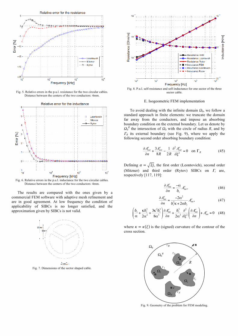
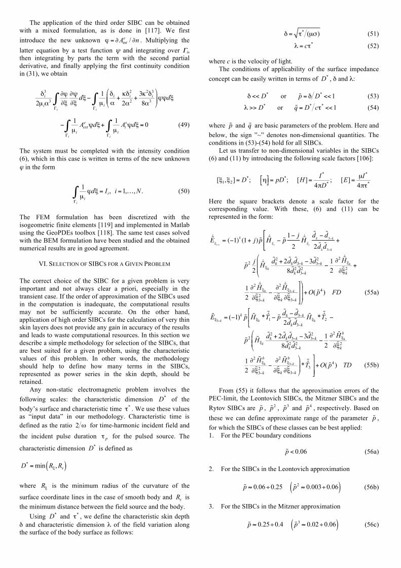
D. BEM numerical results We have implemented the NURBS discretization presented above in a Matlab code, which is mainly based on the GeoPDEs isogeometric software, described in [118]. The code has been used to solve the equations (8)-(16) in several cable configurations, and with the numerical solution we have computed their per unit length (p.u.l.) resistance and inductance, following the procedure described in [113]. The implementation has been first validated by solving the canonical case of two parallel circular copper conductors, with conductivity σ= 5.8 ⋅107 S/m. The diameter of each conductor is 2 mm, and the distance between their centers is 4 mm. The results confirm that high order SIBCs work better at high frequency, and they also increase the frequency range for which the model is valid (Figs. 5-6). In order to deal with a more realistic geometry, we applied the method to the simulation of a three sector-shaped cable with a shield (that we consider infinitely thick). Each sector is made of copper and the same electrical conductivity is also considered for the shield. The dimensions of the cross section of the cable are given in Fig 7. We note that the corners of each sector have been rounded, because the SIBCs discussed here can only be applied in smooth geometries.

Fig. 5. Relative errors in the p.u.l. resistance for the two circular cables. Distance between the centers of the two conductors: 4mm.

Fig. 6. Relative errors in the p.u.l. inductance for the two circular cables.

Distance between the centers of the two conductors: 4mm. The results are compared with the ones given by a commercial FEM software with adaptive mesh refinement and are in good agreement. At low frequency the condition of applicability of SIBCs is no longer satisfied, and the approximation given by SIBCs is not valid.

Fig. 7. Dimensions of the sector shaped cable.

Fig. 8. P.u.l. self-resistance and self-inductance for one sector of the three

sector cable.

E. Isogeometric FEM implementation To avoid dealing with the infinite domain Ω0, we follow a standard approach in finite elements: we truncate the domain far away from the conductors, and impose an absorbing boundary condition on the external boundary. Let us denote by Ω0

R the intersection of Ω0 with the circle of radius R, and by ΓR its external boundary (see Fig. 9), where we apply the following second order absorbing boundary condition:

∂Aexte

∂n+

3Aexte

8R−

12R

∂2 Aexte

∂ξ2= 0 on ΓR (45)

Defining 𝛼 = 2𝑗, the first order (Leontovich), second order (Mitzner) and third order (Rytov) SIBCs on Γi are, respectively [117, 119]:

∂Ainte

∂n=−αδi

Ainte , (46)

∂Ainte

∂n=

−2α2

δi2κ+ 2αδi

Ainte , (47)

δi

α+κδi

2

2α2 +3κ2δi

3

8α3

$

%&&

'

())∂Aint

e

∂n+δi

3

2α3∂2

∂ξ2∂Aint

e

∂n

$

%&&

'

())+ Aint

e = 0 (48)

where 𝜅 = 𝜅 𝜉 is the (signed) curvature of the contour of the cross section.

Fig. 9. Geometry of the problem for FEM modeling.

The application of the third order SIBC can be obtained with a mixed formulation, as is done in [117]. We first introduce the new unknown ϕ = ∂Aint

e / ∂n . Multiplying the latter equation by a test function ψ and integrating over Γi, then integrating by parts the term with the second partial derivative, and finally applying the first continuity condition in (31), we obtain

δi3

2µ iα3

Γi

∫ ∂ϕ∂ξ∂ψ∂ξ

dξ−Γi

∫ 1µ i

δi

α+κδi

2

2α2 +3κ2δi

3

8α3

+

,--

.

/00ϕψdξ

−

Γi

∫ 1µ i

Aexte ψdξ+

Γi

∫ 1µ i

Aisψdξ = 0 (49)

The system must be completed with the intensity condition (6), which in this case is written in terms of the new unknown ϕ in the form

Γi

∫ 1µ iϕdξ = Ii , i =1,…, N . (50)

The FEM formulation has been discretized with the isogeometric finite elements [119] and implemented in Matlab using the GeoPDEs toolbox [118]. The same test cases solved with the BEM formulation have been studied and the obtained numerical results are in good agreement.

VI. SELECTION OF SIBCS FOR A GIVEN PROBLEM The correct choice of the SIBC for a given problem is very important and not always clear a priori, especially in the transient case. If the order of approximation of the SIBCs used in the computation is inadequate, the computational results may not be sufficiently accurate. On the other hand, application of high order SIBCs for the calculation of very thin skin layers does not provide any gain in accuracy of the results and leads to waste computational resources. In this section we describe a simple methodology for selection of the SIBCs, that are best suited for a given problem, using the characteristic values of this problem. In other words, the methodology should help to define how many terms in the SIBCs, represented as power series in the skin depth, should be retained. Any non-static electromagnetic problem involves the following scales: the characteristic dimension D* of the body’s surface and characteristic time τ* . We use these values as “input data” in our methodology. Characteristic time is defined as the ratio 2 ω for time-harmonic incident field and the incident pulse duration τ p for the pulsed source. The

characteristic dimension D* is defined as

D* =min Rξ , Rs( ) where Rξ is the minimum radius of the curvature of the

surface coordinate lines in the case of smooth body and Rs is the minimum distance between the field source and the body. Using D* and τ* , we define the characteristic skin depth δ and characteristic dimension λ of the field variation along the surface of the body surface as follows:

δ = τ* (µσ) (51)

λ = cτ* (52) where c is the velocity of light. The conditions of applicability of the surface impedance concept can be easily written in terms of D* , δ and λ:

δ << D* or !p = δ D* <<1 (53)

λ >> D* or !q = D* cτ* <<1 (54) where !p and !q are basic parameters of the problem. Here and below, the sign ”~” denotes non-dimensional quantities. The conditions in (53)-(54) hold for all SIBCs. Let us transfer to non-dimensional variables in the SIBCs (6) and (11) by introducing the following scale factors [106]:

[ξ1,ξ2]= D*; η"# $%= pD*;

[H ]= I *

4πD* ; [E]= µI *

4πτ*

Here the square brackets denote a scale factor for the corresponding value. With these, (6) and (11) can be represented in the form:

!"Eξ3−k= (−1)k (1+ j) !p !"H

ξ k− !p

1− j

2!"Hξ k

!dk −!d3−k

2 !dk!d3−k

+#

$%

!p2 j2!"Hξk

!dk2 + 2 !dk

!d3−k −3 !d3−k2

8 !dk2 !d3−k

2 −12∂2 !"Hξk

∂!ξk2 +

$

%

&&

12∂2 !"Hξk

∂!ξ3−k2 −

∂2 !"Hξ3−k

∂!ξk ∂!ξ3−k

$

%

&&

'

(

))+O( !p4 ) FD (55a)

!Eξ3−k= (−1)k !p !Hξk

* !T1 − !p!dk − !d3−k

2 !dk!d3−k

!Hξk* !T2 −

#

$%

!p2 !Hξk

!dk2 + 2 !dk

!d3−k −3 !d3−k2

8 !dk2 !d3−k

2 −12∂2 !Hξk

b

∂!ξk2

$

%&&

12∂2 !Hξk

b

∂!ξ3−k2 −

∂2 !Hξ3−kb

∂!ξk ∂!ξ3−k

$

%&&* !T3

'

())+O( !p4 ) TD (55b)

From (55) it follows that the approximation errors of the PEC-limit, the Leontovich SIBCs, the Mitzner SIBCs and the Rytov SIBCs are !p , !p

2 , !p3 and !p

4 , respectively. Based on these we can define approximate range of the parameter !p , for which the SIBCs of these classes can be best applied: 1. For the PEC boundary conditions

!p < 0.06 (56a)

2. For the SIBCs in the Leontovich approximation

!p ≈ 0.06÷0.25 !p2 ≈ 0.003÷0.06( ) (56b)

3. For the SIBCs in the Mitzner approximation

!p ≈ 0.25÷0.4 !p3 ≈ 0.02÷0.06( ) (56c)

4. For the SIBCs in the Rytov approximation

!p ≈ 0.4÷0.5 !p4 ≈ 0.03÷0.06( ) (56d)

The range of the parameter !q can be defined as

!q < 0.06 (57)

Under the definition (56)-(57) the approximation error due to using the SIBCs will not exceed 6%. As an example we considered a pair of identical copper parallel conductors with circular cross section where equal and opposite directed pulses of current 1 A are flowing from an external source as shown in Fig. 10. The radius of each conductor and the distance between the conductors were taken equal to 0.1 m (characteristic value D* ). Under these conditions the current density has only one component directed along the conductors. To illustrate the theory, the distributions of the surface current density over one half of the cross section of one conductor were calculated for the following current pulses:

τ* =10−3 s ( !p = 3.7 ⋅10−2 and !q = 3.3⋅10−7 ). From (56)-(57)

it follows that the PEC-conditions are suitable for this problem. Figure 10 shows that the use of the SIBC of the next order (Leontovich’s SIBC) will not provide significant increase in the accuracy of the results (the difference between the curves does not exceed 4%).

τ* =10−2 s ( !p =1.2 ⋅10−1 and !q = 3.3⋅10−8 ). In this case the

Leontovich SIBC seems to be optimal. From Fig. 11 it follows that the difference between the curves obtained using the PEC- and Leontovich conditions is about 15% whereas application of the Mitzner SIBC increases the accuracy by only 2%. 3. τ

* =10−1 s ( !p = 3.7 ⋅10−1 and !q = 3.3⋅10−9 ). Figure 12 shows that the use of the Leontovich SIBC leads to an unacceptable computational error (about 18%). On the other hand, the difference between the curves obtained in the Mitzner and Rytov approximations does not exceed 3%. Therefore, in this problem it is necessary to use the Mitzner SIBC as the methodology predicts. Note that the methodology employs only two parameters of the problem, and neglects such factors as the shape of the incident pulse. For estimation of the required order of SIBC in more complex, ”grey areas”, application of a more detailed methodology is recommended [106]

Fig. 10. Distribution of the surface current density over the conductor surface

Fig. 11. Distribution of the surface current density over the conductor surface

Fig. 12. Distribution of the surface current density over the conductor surface

VII. ACKNOWLEDGEMENTS

The authors gratefully acknowledge the following: 1. Rafael Vásquez and Annalisa Buffa of the Institute of

Applied Mathematics and Computer Technology of Pavia for their work on the implementation in the BEM context using NURBs as well as in the isogeometric FEM presented above.

2. Olivier Moreau and Valentin Costan from Electricite de France for the support afforded and the results in nondestructive evaluation presented in this work.

3. Stephane Clenet, Yvonnick Le Menach, Thomas Henneron and Francis Piriou from L2EP, Lille, for their help in implementation of SIBCs in code Carmel and for facilitating some of the results presented here.

VIII. CONCLUSIONS

The surface impedance boundary conditions described above and the examples given show the extent of applicability of SIBCs. The main characteristics of the SIBCs are their modular nature with respect to order and the fact that they can be implemented in existing software with little if any additional complexity. In addition, one can estimate the required order a-priory from properties of the geometry and frequency. Although SIBCs for anisotropic media and for coated conductors have been reported, the issue of SIBCs for nonlinear media remains open and is the subject of current work.

0,0 0,1 0,2 0,3

0,5

1,0

1,5

2,0

2,5

3,0

3,5

4,0I(t)

b

ba

τ∗ = 10-3 s

(p = 0.037)

C

B B PEC-limit C Leontovich's SIBC

surfa

ce c

urre

nt d

ensi

ty J

, A/m

surface coordinate υ, m

I(t)2D*

aυ

0,0 0,1 0,2 0,3

0,5

1,0

1,5

2,0

2,5

3,0

3,5

4,0

ba

τ∗ = 10-2 s

D

C

B

(p = 0.12)

B PEC-limit C Leontovich's SIBC D Mitzner's SIBC

surfa

ce c

urre

nt d

ensi

ty J

, A/m

surface coordinate υ, m

0,0 0,1 0,2 0,3

0,5

1,0

1,5

2,0

2,5

3,0

3,5

4,0

ba

τ∗ = 10-1 s(p = 0.37)

ED

C

B B PEC-limit C Leontovich's SIBC D Mitzner's SIBC E Rytov's SIBC

surfa

ce c

urre

nt d

ensi

ty J

, A/m

surface coordinate υ, m

IX. REFERENCES [1] O. Lodge, “On lightning, lightning conductors, and

lightning protectors,” Electrical Review, May 1889, p. 518, John Wiley & Sons, NY, pp 210-213.

[2] S.A. Shelkunoff, “The impedance concept and its application to problems of reflection, radiation, shielding and power absorption”, Bell System Technical Journal, Vol. 17, pp.17-48, 1938.

[3] A. Ishimaru, J.D. Rockway, Y. Kuga and S-W. Lee, “Sommerfeld and Zenneck wave propagation for a finitely conducting one-dimensional rough surface”, IEEE Transactions on Antennas Propagations, Vol. 48, No. 9, pp.1475-1484, 2000.

[4] M.A.Leontovich, "On one approach to a problem of the wave propagation along the Earth's surface", Academy of Science. USSR, Series Physics, Vol. 8, pp. 16-22, 1944.

[5] M.A. Leontovich, “On the approximate boundary conditions for the electromagnetic field on the surface of well conducting bodies”, in Investigations of Radio Waves, B.A. Vvedensky Ed., Moscow: Acad. of Sciences of USSR, 1948.

[6] A.N.Shchukin, Propagation of radio waves, Moscow Svyazizdat, 1940.

[7] G.S. Smith, “On the skin effect approximation”, Am. J. Phys., Vol. 58, No. 10, pp. 996-1002, 1990.

[8] S.M. Rytov, “In the oscillations laboratory”, in Memoires to academician Leontovich, Moscow: Nauka, 1996, pp. 40-66 (in Russian).

[9] M. Rytov, “Calculation of skin effect by perturbation method” J. Experimental’noi i Teoreticheskoi Fiziki, Vol. 10, No. 2, pp.180-189, 1940 (in Russian).

[10] S.M. Rytov, “Calcul du skin-effet par la methode des perturbations, Journal of Physics, Vol. II, No. 3, 1940.

[11] C.Brench, "TC-9 Computational EMC", IEEE EMC Society Newsletter, No. 186, p.13, 2000.

[12] E.M.Deeley and J.Xiang, “Improved surface impedance methods for 2-D and 3-D problems”, IEEE Trans. on Magnetics, Vol. 24, No. 1, pp. 209-211, 1988.

[13] J. Sakellaris, G. Meunier, A. Raizer and A. Darcherif, “The impedance boundary condition applied to the finite element method using the magnetic vector potential as state variable: a rigorous solution for high frequency axisymmetric problems”, IEEE Trans. on Magnetics, Vol. 28, No. 2, pp. 1643-1646, 1992.

[14] A.M. El-Sawy Mohamed, “Finite-element variational formulation of the impedance boundary condition for solving eddy current problems”, IEE Proceedings-Science Measurements and Technology, Vol. 142, No. 4, pp. 293-298, 1995.

[15] M. Gyimesi, J.D. Lavers, T. Pawlak and D. Ostergaard, “Impedance boundary condition for multiply connected domains with exterior cicuit conditions”, IEEE Trans. on Magnetics, Vol. 30, No. 5, pp. 3056-3059, 1994.

[16] J. Sakellaris, G. Meunier, X. Brunotte, C.Guerin and J.C.Sabonnadiere, ”Application of the impedance boundary condition in a finite element enviroment using the reduced potential formulation”, IEEE Trans. on Magnetics, Vol. 27, No. 6, pp. 5022-5024, 1991.

[17] S. Subramaniam, M. Feliziani and S.R. Hoole, “Open boundary eddy-current problems using edge elements”, IEEE Trans. on Magnetics, Vol. 2, pp. 1499-1503, No. 2, 1992.

[18] M. Enokizono and T. Todaka, “Approximate boundary element formulation for high-frequency eddy current

problems”, IEEE Trans. on Magnetics, Vol. 29, No. 2, pp. 1504-1507, 1993.

[19] S.A. Holland, G.P. O’Connel and L. Haydock, “Calculating stray losses in power transformers using surface impedance with finite elements”, IEEE Trans. on Magnetics, Vol. 28, No. 2, pp. 1355-1358, 1992.

[20] D. Rodger, P.J. Leonard, H.C.Lai and P.C.Coles, “Finite element modeling of thin skin depth problems using magnetic vector potential”, IEEE Trans. on Magnetics, Vol. 33, No. 2, pp. 1299-1301, 1997.

[21] G. Pan and J. Tan, “General edge element approach to lossy and dispersive structures in anisotropic media”, IEE Proceedings – Microwaves, Antennas and Propagation, Vol. 144, No. 2, pp. 81-90, 1997.

[22] I. Mayergoyz and C. Bedrosian, “On finite element implementation of impedance boundary conditions”, Journal of Applied Physics, Vol. 75, pp. 6027-6029, 1994.

[23] S.Yuferev and L.Kettunen, “Implementation of high order surface impedance boundary conditions using vector approximating functions”, ”, IEEE Trans. on Magnetics, Vol. 36, No. 4, pp. 1606-1609, 2000.

[24] C. Guerin, G. Tanneau and G. Meunier, “3D eddy current losses calculation in transformer tanks using the finite element method”, IEEE Trans. on Magnetics, Vol. 29, No. 2, pp. 1419-1422, 1993.

[25] J. Tan and G. Pan, “A new edge element analysis of dispersive waveguide structures”, IEEE Transactions on Microwave Theory and Thechniques, Vol. 43, No. 11, pp. 2600-2607, 1995.

[26] S.M. Mimoune, J. Fouladgar, A. Chentouf and G. Develey, “A 3D impedance calculation for an induction heating system for materials with poor conductivity”, IEEE Trans. on Magnetics, Vol. 32, No. 3, pp. 1605-1608, 1996.

[27] W. Mai and G. Henneberger, “Field and temperature calculations in transverse flux inductive heating devices heating non-parametric materials using surface impedance formulations for non-linear eddy-current problems”, IEEE Trans. on Magnetics, Vol. 35, No. 3, pp. 1590-1593, 1999.

[28] J. Nerg and J. Partanen, “A simplified FEM based calculation model for 3-D induction heating problems using surface impedance formulations”, IEEE Trans. on Magnetics, Vol. 37, No. 5, pp. 3719-3722, 2001.

[29] A. Darcherif, A. Raizer, J. Sakellaris and G. Meunier, “On the use of the surface impedance concept in shielded and multiconductor cable characterization by the finite element method”, IEEE Trans. on Magnetics, No. 2, Vol. 2, pp. 1446-1449, 1992.

[30] Z. Badics, Y. Matsumoto, K. Aoki and F. Nakayasu, “Effective probe response calculation using impedance boundary condition in eddy current NDE problems with massive conducting regions present”, IEEE Trans. on Magnetics, Vol. 32, No. 3, pp. 737-740, 1996.

[31] K.R. Davey, “Shell impedance conditions for steady state and transient eddy current problems”, IEEE Trans. on Magnetics, Vol. 25, No. 4, pp. 3007-3009, 1989.

[32] D. Zheng and K.R. Davey, “A boundary element formulation for thin shell problems”, IEEE Trans. on Magnetics, Vol. 32, No. 3, pp. 675-677, 1996.

[33] D. Rodger, P.J. Leonard, H.C.Lai and R.J. Hill-Cottingham, “Surface elements for modeling eddy currents in high permeability materials”, IEEE Trans. on Magnetics, Vol. 27, No. 6, pp. 4995-4997, 1991.

[34] C. Guerin, G. Tanneau, G. Meunier, P. Labie, T. Ngnegueu and M. Sacotte, “A shell element for

computing 3D eddy currents – application to transformers”, IEEE Trans. on Magnetics, Vol. 31, No. 3, pp. 1360-1363, 1995.

[35] L. Krahenbuhl and D. Muller, “Thin layers in electrical engineering. Example of shell models in analyzing eddy-currents by boundary and finite element methods”, IEEE Trans. on Magnetics, Vol. 29, No. 2, pp. 1450-1455, 1993.

[36] S. Subramaniam and S.R. Hoole, “The impedance boundary condition in the boundary element vector potential formulation”, IEEE Trans. on Magnetics, Vol. 4, pp. 2503-2505, Nov 1988.

[37] P. Dular, V. Peron, R. Perrussel, L. Krahenbuhl and C. Geuzaine, “Perfect conductor and impedance boundary condition correction via a finite element subproblem model,” IEEE Transactions on Magnetics, vol. 50, no. 2, 2014.

[38] M.T. Ahmed, J.D. Lavers and P.E. Burke, “On the use of the impedance boundary condition with an indirect boundary formulation”, IEEE Transactions on Magnetics, Vol. 24, No. 6, pp. 2512-2514, 1988.

[39] M.T. Ahmed, J.D. Lavers and P.E. Burke, “Direct BIE formulation for skin and proximity effect calculation with and without the use of the surface impedance approximation”, IEEE Trans. on Magnetics, Vol. 25, pp. 3937-3939, Sep. 1989.

[40] K. Ishibashi, “Eddy current analysis by boundary element method utilizing impedance boundary condition”, IEEE Trans. on Magnetics, Vol. 31, No. 3, pp.1500-1503, 1995.

[41] T.E. van Deventer, P. Katehi and A. Cangellaris, “An integral equation method for the evaluation of conductor and dielectric losses in high-frequency interconnects”, IEEE Transactions on Microwave Theory and Techniques, Vol. 37, No. 12, 1964-1972, 1989.

[42] H. Tsuboi, K. Sue and K. Kunisue, “Surface impedance method using boundary elements for exterior regions”, IEEE Transactions on Magnetics, Vol. 27, No. 5, pp.4118-4121, 1991.

[43] A.A. Kishk and R.K. Gordon, “Electromagnetic scattering from conducting bodies of revolution coated with thin magnetic materials”, IEEE Transactions on Magnetics, Vol. 30, No. 2, pp. 3152-3155, 1994.

[44] A.H. Chang. K.S. Yee and J. Prodan, “Comparison of different integral equation formulations for bodies of revolution with anysotropic surface impedance boundary conditions”, IEEE Transactions on Antennas and Propagation, Vol. 40, No. 8, pp. 989-991, 1992.

[45] A. Bendali, M’B. Fares and J. Gay, “A boundary-element solution of the Leontovich problem”, IEEE Transactions on Antennas and Propagation, Vol. 47, No. 10, pp. 1597-1605.

[46] P.L. Huddleston, “Scattering by finite, open cylinders using approximate boundary conditions”, IEEE Transactions on Antennas and Propagation, Vol. 37, No. 2, pp. 253-257, 1989.

[47] O. Sterz and C. Schwab, “A scalar boundary integrodifferential equation for eddy current problems using an impedance boundary condition”, Comput. Vis. Sci., Vol. 3, pp. 209-217, 2001.

[48] H.C. Jayatilaka and I.R. Ciric, “Performance of surface impedance integral equations for quasi-stationary field analysis in axisymmetric systems”, IEEE Transactions on Magnetics, Vol. 40, No. 2, pp. 1350-1353, 2004.

[49] S. Yuferev and V. Yuferev, “Calculation of the electromagnetic field diffusion in a system of parallel

conductors”, Soviet Physics Technical Physics Journal, Vol. 36, pp. 1208-1211, 1991.

[50] S. Yuferev, “Generalized BIE-BLA formulation of skin and proximity effect problems for an arbitrary regime of the magnetic field generation”, Second International IEE Conference on Computation in Electromagnetics, IEE Conference Publication No. 384, pp. 307-310, 1994.

[51] S. Yuferev and N. Ida, “Application Of Approximate Boundary Conditions To Electromagnetic Transient Scattering Problems”, Third Intern. IEE Conference on Computation in Electromagnetics, IEE Conference Publication No. 420, pp. 51-56, 1996.

[52] S. Yuferev and N. Ida, “Efficient implementation of the time domain surface impedance boundary conditions for the boundary element method”, IEEE Trans. on Magnetics, Vol. 34, No. 2, pp. 2763-2766, 1998.

[53] J.A. Roden and S.D. Gedney, “The efficient implementation of the surface impedance boundary condition in general curvilinear coordinates”, IEEE Transactions on Microwave Theory and Techniques, Vol. 47, No. 10, pp. 1954-1963, 1999.

[54] J.G. Maloney and G.S. Smith “The use of surface impedance concepts in the finite-difference time-domain method”, IEEE Transactions on Antennas and Propagation, Vol. 40, No. 1, pp. 38-48, 1992.

[55] K.S. Yee, K. Shlager and A.H. Chang “An algorithm to implement a surface impedance boundary condition for FDTD”, IEEE Transactions on Antennas and Propagation, Vol. 40, No. 7, pp. 833-837, 1992.

[56] C.F. Lee, R.T. Shin and J.A. Kong “Time domain modeling of impedance boundary condition”, IEEE Transactions on Microwave Theory and Techniques, Vol. 40, No. 9, pp. 1847-1851, 1992.

[57] S. Kellahi and B.J.J ecko “Implementation of a surface impedance formalism at oblique incidence in FDTD method”, IEEE Transactions on Electromagnetic Compatibility, Vol. 35, No. 3, pp. 347-356, 1993.

[58] K.S. Oh and J.E. Schutt-Aine “An efficient implementation of surface impedance boundary conditions for the finite-difference time-domain method”, IEEE Transactions on Antennas and Propagation, Vol. 43, No. 7, pp. 660-666, 1995.

[59] C.F. Lee, R.T.Shin and J.A. Kong, “Time domain modeling of impedance boundary condition”, IEEE Transactions on Micrwave Theory and Techniques, Vol. 40, No. 9, pp. 1847-1851, 1992.

[60] J.H. Beggs, R.J. Lubbers, K.S. Yee and K.S. Kunz, “Finite-difference time-domain implementation of surface impedance boundary conditions”, IEEE Transactions on Antennas and Propagation, Vol. 40, No. 1, pp. 49-56, 1992.

[61] C.W. Penney, R.L. Luebbers and J.W. Schuster, “Scattering from coated targets using a frequency-dependent, surface impedance boundary condition in FDTD”, IEEE Transactions on Antennas and Propagation, Vol. 44, No. 4, pp. 434-443, 1996.

[62] K.S. Yee and J.S. Chen, “Impedance boundary condition simulation in the FDTD/FVTD hybrid”, IEEE Transactions on Antennas and Propagation, Vol. 45, No. 6, pp. 921-925, 1997.

[63] J.H. Beggs, “A FDTD surface impedance boundary condition using Z-transform”, Applied Computational Electromagnetics Society Journal, Vol. 13, No. 3, pp. 14-24, 1998.

[64] M.K. Karkkainen and S.A. Tretiakov, ”Finite-difference time domain model of interfaces with metals

and semiconductors based on a higher order surface impedance boundary conditions”, IEEE Transactions on Antennas and Propagation, Vol. 51, No. 9m pp. 2448-2455, 2003.

[65] M.K. Karkkainen, “FDTD surface impedance model for coated conductors”, IEEE Transactions on Electromag. Compatibility, Vol. 46, No. 2, pp. 222-233, 2004.

[66] P.G. Petropoulos, Approximating the surface impedance of a homogeneous lossy half-soace: an example of “dialable” accuracy”, IEEE Transactions on Antennas and Propagation, Vol. 50, No. 7, pp. 941-943, 2002.

[67] R. Makinen, “An efficient surface-impedance boundary condition for thin wires of finite conductivity”, IEEE Transactions on Antennas and Propagation, Vol. 52, No. 12, 3364-3372, 2004.

[68] S.Yuferev, N. Farahat, N.Ida, “Use of the perturbation technique for implementation of surface impedance boundary conditions for the FDTD method”, IEEE Transactions on Magnetics, Vol. 36, No. 4, pp.942 – 945, 2000.

[69] N. Farahat, S.Yuferev, N.Ida, “High order surface impedance boundary conditions for the FDTD method”, IEEE Transactions on Magnetics, Vol. 37, No. 5, pp.3242 – 3245, 2001.

[70] L. Lin and C. Xiang, “Losses calculation in transformer tie plate using the finite element method”, IEEE Transactions on Magnetics, Vol. 34, No. 5, pp. 3644-3647, 1998.

[71] Y. Higuchi and M. Koizumi, “Integral equation method with surface impedance model for 3D eddy current analysis in transformers”, IEEE Transactions on Magnetics, Vol. 36, No. 4, pp. 774-779, 2000.

[72] C. Guerin, G. Meunier and G. Tanneau, “Surface impedance for 3D non-linear eddy current problems – application to loss computation in transformers”, IEEE Transactions on Magnetics, Vol. 32, No. 3, pp. 808-811, 1996.

[73] A. Weisshaar, “Impedance boundary method of moments for accurate and efficient analysis of planar graded-index optical waveguides”, Journal of Lightwave Technology, Vol. 12, No. 11, pp.1943-1951, 1994.

[74] M.S. Islam, E. Tuncer and D.P. Neikirk, “Calculation of conductor loss in coplanar waveguide using conformal mapping”, Electronic Letters, Vol. 29, No. 13, pp. 1189-1191, 1993.

[75] K. Yoshitomi and H.R. Sharobim, “Radiation from a rectangular waveguide with a lossy flange”, IEEE Transactions on Antennas and Propagation, Vol. 42, No. 10, pp. 1398-1403, 1994.

[76] K.A. Remley and A. Weisshaar, “Impedance boundary method of moments with extended boundary conditions”, Journal of Lightwave Technology, Vol. 13, No. 12, pp. 2372-2377, 1995.

[77] F. Bioul, F. Dupret, “Application of asymptotic expansions to model two-dimensional induction heating systems. Part I: calculation of electromagnetic field distribution”, IEEE Transactions on Magnetics, Vol. 41, No. 9, pp. 2496-2505, 2005.

[78] F. Bioul, F. Dupret, “Application of asymptotic expansions to model two-dimensional induction heating systems. Part II: calculation of equivalent surface stresses and heat flux”, IEEE Transactions on Magnetics, Vol. 41, No. 9, pp. 2506-2514, 2005.

[79] W. Thiel, “A surface impedance approach for modeling transmission line losses in FDTD”, IEEE Microwave

and Guided Wave Letters, Vol. 10, No. 3, pp. 89-91, 2000.

[80] S. Kim and D.P. Neikirk, “Time domain multiconductor transmission line analysis using effective internal impedance,”IEEE 6th Topical Meeting on Electronic Packaging, IEEE Cat. Number 97TH8318, San Jose, CA, October 27-29, pp. 255-258. (EPE97_reprint.pdf)

[81] E.M. Deeley, “Microstrip calculations using an improved minimum-order boundary element method”, IEEE Transactions on Magnetics, Vol. 30, No. 5, pp. 3753-3756, 1994.

[82] I.P. Theron and J.H. Cloete, “On the surface impedance used to model the conductor losses of microstrip structures”, IEE Proceedings-Microwaves, Antennas and Propagation, Vol. 142, No. 1, pp.35-40, 1995.

[83] L.L. Lee, W.G. Lyons, T.P. Orlando, S.M. Ali and R.S. Withers, “Full-wave analysis of superconducting microstrip lines on anisotropic substrates using equivalent surface impedance approach”, IEEE Transactions on Microwave Theory and Techniques, Vol. 41, No. 12, pp. 2359-2367, 1993.

[84] D. De Zutter, L. Knockaert, “Skin Effect Modeling Based on a Differential Surface Admittance Operator”, IEEE Trans. Microwave Theory Techn., Vol. 53, No. 8, pp. 2526-2538, 2005.

[85] K. Adamiak, G.E. Dawson and A.R. Eastham, “Application of impedance boundary conditions in finite element analysis of linear motors”, IEEE Transactions on Magnetics, Vol. 27, No. 6, pp. 5193-5195, 1991.

[86] V.C. Silva, Y. Marechal and A. Foggia, “Surface impedance method applied to the prediction of eddy currents in hydrogenerator stator end regions”, IEEE Transactions on Magnetics, Vol. 31, No. 3, pp. 2072-2075, 1995.

[87] J.F. Eastham, D. Rodger, H.C. Lai and H. Nouri, “Finite element calculation of fields around the end region of a turbine generator test rig”, IEEE Transactions on Magnetics, Vol. 29, No. 2, pp. 1415-1418, 1993.

[88] A. Sebak and L. Shafai, “Scattering from arbitrarily-shaped objects with impedance boundary conditions”, IEE-Proceedings-H, Vol. 136, No. 5, pp. 371-376, 1989.

[89] M. Osuda and A. Sebak, “Scattering from lossy dielectric cylinders using a multifilament current model with impedance boundary conditions”, IEE Proceedings-H, Vol. 139, No. 5, pp. 429-434, 1992.

[90] T.B.A. Senior and J.L. Volakis, “Generalized impedance boundary conditions in scattering”, Proceedings of the IEEE, Vol. 79, No. 10, pp. 1413-1420, 1991.

[91] A.A. Kishk, “Electromagnetic scttering from composite objects using mixture of exact and impedance boundary conditions”, IEEE Transactions on Atennas and Propagation, Vol. 39, No. 6, pp. 826-833, 1991.

[92] R.D. Graglia, P.L.E. Uslenghi, R. Vitiello and U. D’Elia, “Electromagnetic scttering for oblique incidence on impedance bodies of revolution”, IEEE Transactions on Antennas and Propagation, Vol. 43, No. 1, pp. 11-26, 1995.

[93] L.N. Medgyesi-Mitschang and J.M.Putnam, “Integral equation formulations for imperfectly conducting scatters”, IEEE Transactions on Antennas and Propagation, Vol. 33., No. 2, pp. 206-214, 1985.

[94] M. D’Amore and M.S. Sarto, “Theoretical and experimental chracterization of the EMP-interaction

with composite-metallic enclosures”, IEEE Transactions on Electromagnetic Compatibility, Vol. 42, No. 1, pp. 152-163, 2000.

[95] C. Yang, V. Jandhyala, “A time-domain surface integral technique for mixed electromagnetic and circuit simulation”, IEEE Transactions on Advanced Packaging, 2005 (accepted for publication).

[96] M.S. Sarto, “A new model for the FDTD analysis of the shielding performances of thin composite structures”, IEEE Transactions on Electromagnetic Compatibility, Vol. 41, No. 4, pp. 298-306, 1999.

[97] H. Sahinturk, “On the reconstruction of inhomogeneous surface impedance of cylindrical bodies”, IEEE Transactions on Magnetics, Vol. 40, No. 2, pp. 1152-1155, 2004.

[98] R. Grimberg, H. Mansir, J.L. Muller and A. Nicolas, “A surface impedance boundary condition for 3-D non destructive testing odeling,” IEEE Transactions on Magnetics, Vol. MAG-22, No. 5, September, pp. 1272-1274, 1986.

[99] T.H.Fawzi, M.T.Ahmed and P.E.Burke, “On the use of the surface impedance boundary conditions in eddy current problems”, IEEE Transactions on Magnetics, Vol. 21, No. 5, pp. 1835-1840, 1985.

[100] F.-Z. Louai, D. Benzerga and M. Feliachi, “A 3D finite element analysis coupled to the impedance boundary condition for the magnetodynamic problem in radiofrequency plasma devices”, IEEE Transactions on Magnetics, Vol. 32, No. 3, pp. 812-815, 1996.

[101] A. Helaly, E.A. Soliman and A.A. Megahed, “Electromagnetic waves scattering by non-uniform plasma cylinder”, IEE-Proceedings – Microwaves, Antennas and Propagation, Vol. 144, No. 2, pp. 61-66, 1997.

[102] M.R. Ahmed and J.D Lavers, “Boundary element analysis of the electromagnet casting mould”, IEEE Transactions on Magnetics, Vol. 25, No. 4, pp. 2843-2845, 1989.

[103] B. Dumont and A. Gagnoud, “3D finite element method with impedance boundary condition for the modeling of molten metal shape in electromagnetic casting”, IEEE Transactions on Magnetics, Vol. 36, No. 4, pp. 1329-1332, 2000.

[104] J.R. Wait, “The ancient and modern history of EM ground-wave propagation”, IEEE Antennas and Propagation Magazine, Vol. 40, No. 5, pp. 7-24, 1998.

[105] C. R. I. Emson and J. Simkin, “An optimal method for 3-D eddy currents,” IEEE Transactions on Magnetics, Vol. MAG-21, No. 6, November, pp. 2231-2234, 1985.

[106] S. Yuferev and N. Ida, Surface Impedance Boundary Conditions, CRC Press, Boca Raton, June 2010.

[107] O. Moreau, F. Buvat, C. Gilles-Pascaud, C. Reboud: "An Approach for Validating NDT Eddy Currents Simulation Codes", 7th International Conference on NDE in relation to structural integrity for nuclear and pressurized components, Yokohama, May 2009.

[108] M. Piriou, S. W. Glass: "Steam Generator Secondary Side Deposit-NDE Method for Support Plate Clogging", 7th International Conference on NDE in relation to structural integrity for nuclear and pressurized components, Yokohama, May 2009.

[109] O. Moreau, V. Costan, J.M. Devinck, and N. Ida, “Finite Element Modeling of Support Plate Clogging-up in Nuclear Plant Steam Generator,” Proceedings of the 8th International Conference on NDE in Relation to

Structural Integrity for Nuclear and Pressurised Components, 29 September to 1 October 2010, Berlin, Germany (PDF).

[110] http://code-carmel.univ-lille1.fr/ (an FEM code developed jointly by the EDF R&D and the L2EP Laboratory at the University of Lille, a code destined to become open-source in the near future)

[111] T. J. R. Hughes, J. A. Cottrell, and Y. Bazilevs, “Isogeometric analysis: CAD, finite elements, NURBs, exact geometry and mesh refinement,” Computational Methods in Applied Mechanics and Engineering, Vol. 194, No. 39-41, pp. 4135-4195, 2005.

[112] R. Vázquez and A. Buffa, “Isogeometric analysis in electromagnetics: B-splines approximation,” Computational Methods in Applied Mechanics and Engineering, vol. 199, no. 17-20, pp. 1143-1152, 2010.

[113] L. Di Rienzo, S. Yuferev, and N. Ida, "Computation of the impedance matrix of multiconductor transmission lines using high order surface impedance boundary conditions," IEEE Transactions on Electromagnetic Compatibility, vol. 50, No. 4, November, pp. 974-984, 2008.

[114] S. Barmada, L. Di Rienzo, N. Ida, and S. Yuferev, “The use of the surface impedance boundary condition in time domain problems: numerical and experimental validation,” Applied Computational Electromagnetics Society Journal, vol. 19, No. 2, July 2004, pp. 76-83.

[115] S. Barmada, L. Di Rienzo, N. Ida, and S. Yuferev “Time domain surface impedance concept for low frequency electromagnetic problems—part II: application to transient skin and proximity effect problems in cylindrical conductors,” IEE Proceedings – Science, Measurement and Technology, vol. 152, No. 5, September, pp. 207-216, 2005.

[116] C. Brebbia, The Boundary Element Method for Engineers, London, U.K., Pentech, 1980.

[117] H. Haddar, P. Joly, and H.-M. Nguyen, “Generalized impedance boundary conditions for scattering by strongly absorbing obstacles: the scalar case,” Math. Models Methods in Applied Science, vol. 15, no.. 88, pp. 1273-1300, 2005.

[118] C. de Falco, A. Reali, and R. Vázquez, “GeoPDEs: a research tool for isogeometric analysis of PDEs,” Advances in Engineering Software, vol. 42, no. 12, pp. 1020-1034, 2011.

[119] R. Vázquez, A. Buffa, and L. Di Rienzo, "Isogeometric FEM implementation of high order surface impedance boundary conditions," to appear in IEEE Transactions on Magnetics, 2014.

AUTHORS NAME AND AFFILIATION

Sergey S. Yuferev, Infineon Technologies, Siemensstrasse 2,

Vilach, Austria, Sergey.Yuferev@infineon.com Luca di Rienzo, Politecnico di Milano, Dipartimento di

Elettronica, Informazione e Bioingegneria – Sezione Elettrica, Piazza L. da Vinci, 32, Milano, Italy, luca.dirienzo@polimi.it

Nathan Ida, The University of Akron, Department of Electrical and Computer Engineering, Akron, Ohio 44325-3904, USA, ida@uakron.edu