Contents lists available at SciVerse ScienceDirect

Journal of Fluids and Structures

Journal of Fluids and Structures 34 (2012) 123–137

0889-97

http://d

n Corr

E-m

journal homepage: www.elsevier.com/locate/jfs

Surface pressure survey in a parallel triangular tube array

John Mahon, Craig Meskell n

School of Engineering, Trinity College Dublin, Ireland

a r t i c l e i n f o

Article history:

Received 18 August 2011

Accepted 18 May 2012Available online 22 June 2012

Keywords:

Fluidelastic instability

Fluid forces

Flow instability

Jet switching

Heat exchanger

Tube arrays

Bistable flow

46/$ - see front matter & 2012 Elsevier Ltd. A

x.doi.org/10.1016/j.jfluidstructs.2012.05.005

esponding author.

ail address: cmeskell@tcd.ie (C. Meskell).

a b s t r a c t

An experimental parametric study of the surface pressure on a cylinder in the sixth row

of a rotated triangular tube array (P/d¼1.375) with air cross-flow has been conducted.

A range of static displacements were examined. Jet switching was observed in this array

and resulted in large asymmetry in the pressure distribution around the static cylinder

even in a geometrically symmetric configuration. The large fluctuations in lift force due

to jet switching suggest that it should be more seriously considered when designing

against failure. The effect of jet switching on the pressure distribution data was

mitigated by deconstructing the pressure distribution into two modes. Forces were

calculated from the pressure measurements. No simple parameterisation was found for

either the lift or drag force, but it was found that the drag force was only weakly

affected by the tube displacement. The data set presented here compliments the data

previously presented for normal triangular arrays and represents a valuable reference

for validation of simulations and flow-induced vibration models.

& 2012 Elsevier Ltd. All rights reserved.

1. Introduction

Paidoussis (1979) presented details of case studies of flow-induced vibration problems in heat exchangers and nuclearreactors. We are interested in the 33 cases presented on flow induced vibration due to a cross-flow. The flow inducedvibration mechanisms were classified under a number of headings: vortex shedding, vortex shedding and acousticresonance, fluidelastic instability, turbulent buffeting, and unknown. It is generally accepted that the mechanism offluidelastic instability has the greatest potential to cause damage and it occurs when a critical velocity is reached. Themechanism has the potential to destroy a unit in a few hundred hours of operation. As such, the operating cross-flowvelocity chosen should be on the conservative side compared to the fluidelastic threshold. However, as the fluid mechanicsare not fully understood it is difficult to determine whether the design cross-flow velocity is conservative or not even if thecross-flow velocity does not cause the onset of fluidelastic instability. Furthermore, even if the cross-flow velocity issufficiently low so that fluidelastic instability does not occur, the fluidelastic forces are not zero. These fluid stiffness andfluid damping forces are important in assessing the response of the system to turbulent buffeting (e.g. Piteau et al., 2012).

The mechanism responsible for fluidelastic instability in tube arrays has been described by three theoretical frameworks: the‘‘wavy-wall’’ model (Lever and Weaver, 1986); the quasi-static model (Connors, 1970); and the quasi-steady model (Price andPaidoussis, 1984). There are also a number of empirical models. In addition, there have been a number of numerical simulations offlow through heat exchangers tube arrays and fluideleastic instability using large eddy simulation, Reynolds averaged NavierStokes and vortex methods (e.g. Beale and Spalding, 1999; Kassera et al., 1995; Sweeney and Meskell, 2003). Indeed,computational approach to studying tube arrays is not confined to heat exchangers; recently, Hillewaere et al. (2012) haveused unsteady RANS to model the flow around a densely packed array of circular storage tanks. These models for fluidelastic

ll rights reserved.

Nomenclature

a pitch velocity constant [P/(P�d)]b,c,K1�3 model constantsCD drag coefficientCL lift coefficientCP mean pressure coefficientd tube diameterf frequency (Hz)FD drag forceFL lift forceFy fluidelastic forcel tube lengthm tube massmr mass damping parameter ð ¼md=rd2

Þ

P pitchP/d pitch ratioPy mean pressure at a given position anglePo mean pressure at stagnation pointRe Reynolds numberUr reduced critical gap velocity (¼Upc/fd)y tube displacement_y tube velocityy/d dimensionless tube displacement (yn)d logarithmic decrementy position angler fluid density (air)t time delayo frequency (rad/s)oo natural frequency (rad/s)

J. Mahon, C. Meskell / Journal of Fluids and Structures 34 (2012) 123–137124

instability, whether semi-empirical or numerical, are based on very different assumptions of the fluid mechanics. However, theapproach for validating these models depend primarily on comparison of predicted critical velocity to experimental values.Unfortunately, while this threshold is ultimately of greatest interest from a practical point of view, the experimental data availableshow a significant unexplained scatter and hence confidence in model validation is poor. In order to provide an initial validationof the assumptions and predictions of these models, a detailed survey of the surface pressure distribution on a statically displacedcylinder in a rotated triangular tube array has been conducted. While there is already limited pressure data in the literature(Achenbach, 1969; Zdravkovich and Namork, 1980; Zukauskas et al., 1983), pressure distributions were measured for only a fewReynolds numbers. Furthermore, until recently there have been no comprehensive studies of the pressure field around a staticallydisplaced cylinder within a tube array available. Batham (1973) presented a limited study of the pressure distribution around astatically displaced cylinder in an array. The configuration used was a ten row in-line array with pitch ratio of 1.25. It wasreported that tubes in the first three rows were displaced by 0.25 mm which corresponds to � 0:5% tube displacement and thatthe pressure distribution ‘‘completely changed’’. However, no detailed results were presented. More recently, Mahon and Meskell(2009a) presented pressure distributions around a cylinder in three normal triangular tube arrays, for a range of Reynolds numberand static tube displacements. Nonetheless, there is still limited information on parallel (rotated) triangular tube arrays. Thisstudy presents a survey of surface pressure in a parallel triangular tube array with static tube displacement.

2. Experimental set-up

A draw-down wind tunnel was used in these experiments. The test-section dimensions are 750 mm long with a cross-section of 300 mm high�272 mm wide. The flow velocity in the wind tunnel test-section ranged from 2 m/s to 10 m/swith a free stream turbulence intensity of less than 1%. The flow velocity was measured using a pitot-static tube installedupstream of the test section.

The array under test was an eight row rotated triangular array with a pitch ratio of 1.375. A schematic of the test-section is shown in Fig. 1. The tubes are manufactured of aluminium and are 38 mm in diameter. The tubes in the array arerigidly fixed, except for one tube which will be referred to as the instrumented cylinder. The instrumented cylinder has 36pressure taps with a diameter of 1 mm located at the mid-span around the circumference of the cylinder (equispaced at101 intervals). The length of the cylinder assembly within the test section was 298 mm. A schematic illustrating the bulkflow direction and tube position angle (angular position) is shown Fig. 2. Note the position angle is defined as the positive

U P (52.8mm)

d (38mm)

y

x

Fig. 1. Test section schematic: parallel (rotated) triangular array, P/d¼1.375.

Fig. 2. Schematic of position angle.

Table 1Free stream velocities (U), gap velocities (Ug) and Reynolds numbers (Re) tested.

U (m/s) Ug (m/s) Re (�104)

2 7.3 1.97

3 11.0 2.95

4 14.7 3.93

5 18.3 4.91

6 22.0 5.90

7 25.7 6.88

8 29.3 7.86

9 33.0 8.84

10 36.7 9.83

Table 2Tube displacements tested.

y/d (%) 0 1 3 5 7 10 �5

J. Mahon, C. Meskell / Journal of Fluids and Structures 34 (2012) 123–137 125

clockwise angle starting from the front of the cylinder. The tube was mounted on a traverse (located outside the windtunnel) allowing a specific static displacement to be applied to the cylinder. The traverse facilitated fine displacements andthe displacement was monitored with a clock gauge with a precision of 0.01 mm. Displacements were applied in thedirection perpendicular to the flow only (i.e. y direction in Fig. 1).

The instrumented tube was connected to the pressure transducers with short lengths of 2 mm internal diametersilicone tubing. Each pressure tap was monitored with a differential pressure transducer (Honeywell 164PC01D37). Theother port of the pressure transducer was vented to atmosphere. In effect the gauge pressure was measured.

The signals from the pressure transducers were acquired simultaneously at a sample frequency of 1024 Hz. As theprimary focus of this study is the mean pressure distribution, the pressure transducers were calibrated by applying aconstant known pressure. From this, the sensitivity of the pressure transducer was obtained (i.e. a relationship betweenthe output voltage from the pressure transducer due to a known pressure). The other pressure transducers were thencalibrated with respect to this reference pressure transducer. The readings from the pressure transducers were digitisedand logged using an NI 48 channel, 24 bit data acquisition frame. Each channel was simultaneously sampled andautomatically low pass filtered to avoid aliasing. Additional information on the test set-up including schematics andphotographs of the pressure tap tube can be found in Mahon (2008) and Mahon and Meskell (2009a).

3. Results

An eight-row rotated triangular array with a pitch ratio of 1.375 with air cross-flow was investigated. Surface pressuremeasurements on a cylinder in the centre of the sixth row have been obtained for a range of flow velocities and static tubedisplacements. Table 1 details the free stream velocities tested as well as the associated gap velocities and Reynoldsnumbers (based on the gap velocities), while Table 2 outlines the tube displacements tested.

The pressure distribution around the cylinder was non-dimensionalised and the results presented in terms of the meanpressure coefficient, CP

CP ¼ 1�Po�Py1

2rU2

g

, ð1Þ

0 45 90 135 180 225 270 315 360−260

−240

−220

−200

−180

−160

−140

−120

−100

Pre

ssur

e (P

a)

θ

Fig. 3. Mean pressure distribution, y/d¼0% and U¼4 m/s (Re¼3.93�104).

J. Mahon, C. Meskell / Journal of Fluids and Structures 34 (2012) 123–137126

where Po refers to the mean pressure at the stagnation point, Py refers to the local mean static pressure at a given angularposition, Ug is the gap velocity ðUg ¼U½P=ðP�dÞ�Þ and r is the fluid density.1 The pressure coefficient was expressed in thisway since taking the free stream static pressure as the reference pressure was not appropriate as the mean static pressurevaries throughout the array.

The experimental set-up has been validated previously (Mahon and Meskell, 2009a) by measuring the mean pressuredistribution around an isolated cylinder and comparing the results with those in the literature.

3.1. Pressure distribution

Fig. 3 shows the typical mean pressure distribution around a cylinder in the sixth row of the parallel triangular tube arraywith zero static displacement for a record length of 100 s and a sample frequency of 1024 Hz. It is apparent that the pressuredistribution is not symmetric. The asymmetry was significantly larger than that associated with a rotational offset in theposition angle. Asymmetry due to misalignment of the tube’s position can be ruled out as the misalignment would have to bevery large to cause such distortion. Furthermore, when the tests were repeated the pressure distribution changed. Thisbehaviour was also observed at other flow velocities. Hence, the authors are satisfied that the asymmetry in the pressuredistribution was not as a result of misalignment. Mahon and Meskell (2009a) observed large asymmetry in one of the normaltriangular arrays (P/d¼1.58) investigated and this was attributed to bi-stable flow structures. This effect has also been observedby others; for example Zdravkovich and Stonebanks (1990), Indrusiak et al. (2005) and Zdravkovich (1993).

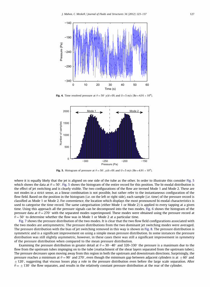
Further investigation revealed that there is a bi-stable flow regime. Fig. 4 shows the time resolved pressure signal aty¼ 501, at a flow velocity of 4 m/s. It is clear that there is significant variation in the pressure signal. Plotting a histogram ofthe signal (Fig. 5), it is apparent that there is a bi-modal flow instability (jet switching). This bi-modal behaviour wasobserved at most flow velocities and tube displacements tested with the exception of flow velocities of 2 and 3 m/s. It ispossible that flow instability was occurring at those velocities but it was not as pronounced as in the other cases and wasmasked by turbulence. Olinto et al. (2009) reported that the bi-modal jet switching did not occur in water flow, but did inair flows at the same Reynolds number, but at higher flow velocity. So, an alternative explanation for an absence of jetswitching at low velocities in this study, might be that there is some minimum flow velocity (i.e. dynamic head) requiredto initiate the jet switching process. The presence of a flow instability (jet switching) complicates the analysis of the dataas the pressure distribution changes from test to test regardless of whether the velocity or displacement parameters arechanged. The mean pressure will show a bias towards one of the modes as the test duration (100 s) is small whencompared to temporal spacing of the jet switching phenomenon which is of the order of tens of seconds. Note that the jetswitching is not periodic, rather the switch from one regime to another occurs intermittently at random intervals.

It was found that generally only two modes exist. If the time record was sufficiently long the mean pressuredistribution would be unbiased. However, as the jet switching is a random intermittent phenomenon with a temporalspacing of tens of seconds, the necessary record length would be prohibitive. Thus, the approach taken to generate the longterm average was to decompose the pressure records into two modes, and to take the average of these two modes. Notethat this does not remove the effect of jet switching; rather it offers the mean pressure distribution for the hypothetical case

1 The gap velocity implicitly assumes a constant tangential velocity along a curvilinear stream tube passing through the array. The actual local

velocity in the region of the tube will vary considerably as will the streamwise component. Nonetheless, use of this gap velocity as the reference velocity

in tube arrays is standard.

0 10 20 30 40 50 60−340

−290

−240

−190

−140

Time (s)

Pre

ssur

e (P

a)

Fig. 4. Time resolved pressure at y¼ 501 y/d¼0% and U¼5 m/s (Re¼4.91�104).

Fig. 5. Histogram of pressure at y¼ 501, y/d¼0% and U¼5 m/s (Re¼4.91�104).

J. Mahon, C. Meskell / Journal of Fluids and Structures 34 (2012) 123–137 127

where it is equally likely that the jet is aligned on one side of the tube as the other. In order to illustrate this consider Fig. 5which shows the data at y¼ 501. Fig. 5 shows the histogram of the entire record for this position. The bi-modal distribution isthe effect of jet switching and is clearly visible. The two configurations of the flow are termed Mode 1 and Mode 2. These arenot modes in a strict sense, as a linear combination is not possible, but rather refer to the instantaneous configuration of theflow field. Based on the position in the histogram (i.e. on the left or right side), each sample (i.e. time) of the pressure record isclassified as Mode 1 or Mode 2. For convenience, the location which displays the most pronounced bi-modal characteristics isused to categorise the time record. The same categorisation (either Mode 1 or Mode 2) is applied to every tapping at a giventime. Using this approach all the pressure signals can be decomposed into the two modes. Fig. 6 shows the histogram of thepressure data at y¼ 2701 with the separated modes superimposed. These modes were obtained using the pressure record aty¼ 501 to determine whether the flow was in Mode 1 or Mode 2 at a particular time.

Fig. 7 shows the pressure distribution of the two modes. It is clear that the two flow field configurations associated withthe two modes are antisymmetric. The pressure distributions from the two dominant jet switching modes were averaged.The pressure distribution with the bias of jet switching removed in this way is shown in Fig. 8. The pressure distribution issymmetric and is a significant improvement on using a simple mean pressure distribution. In some instances the pressuredistribution was still slightly asymmetric, however, in these cases there was still a significant improvement in symmetryof the pressure distribution when compared to the mean pressure distribution.

Examining the pressure distribution in greater detail at y¼ 302401 and 320–3301 the pressure is a maximum due to theflow from the upstream tubes impinging on to the tube (reattachment of the shear layers separated from the upstream tubes).The pressure decreases upon moving away from this region in both the upstream and downstream directions. Surprisingly, thepressure reaches a minimum at y¼ 901 and 2701, even though the minimum gap between adjacent cylinders is at 7601 and71201, suggesting that viscous losses play a role in the pressure distribution even before the large scale separation. Aftery¼71301 the flow separates, and results in the relatively constant pressure distribution at the rear of the cylinder.

Fig. 6. Histogram of pressure at y¼ 2701, y/d¼0% and U¼5 m/s (Re¼4.91�104) Red - Mode 1, Green - Mode 2, Blue - Combination of both modes. (For

interpretation of the references to color in this figure legend, the reader is referred to the web version of this article.)

0 45 90 135 180 225 270 315 360−260

−240

−220

−200

−180

−160

−140

−120

−100

Pre

ssur

e (P

a)

θ

Fig. 7. Mode 1 and Mode 2 of the pressure distribution, y/d¼0% and U¼4 m/s.

0 45 90 135 180 225 270 315 360−260

−240

−220

−200

−180

−160

−140

−120

Pre

ssur

e (P

a)

θ

Fig. 8. Mode average pressure distribution, y/d¼0% and U¼4 m/s.

J. Mahon, C. Meskell / Journal of Fluids and Structures 34 (2012) 123–137128

J. Mahon, C. Meskell / Journal of Fluids and Structures 34 (2012) 123–137 129

Figs. 9 and 10 present pressure coefficient data for a range of Reynolds numbers at y/d¼0% and y/d¼5%, respectively.The pressure distribution around the tube changes with Reynolds number. At Re¼7–8�104 (U¼7–8 m/s) the locations ofminimum and maximum pressure change suggesting a change in the flow structure. Furthermore, at the rear of thecylinder the point of separation moves closer to the rear of the cylinder. It is clear that pressure coefficient curves do notcollapse and that there is a Reynolds number dependency, hence, the results discussed below are presented in terms ofgauge pressure as there is limited benefit to non-dimensionalising the pressure distribution with dynamic head.

3.2. Tube displacement

Static tube displacements of 1%, 3%, 5%, 7% and 10% tube diameter were examined. Figs. 11–13 show pressuredistribution around a cylinder in the sixth row for the range of static tube displacements at flow velocities of 4, 6 and 8 m/s,respectively. The effect of tube displacement is apparent. The region y¼ 302401 shows a decrease in pressure whereas theregion y¼ 32023301 on the opposite side of the cylinder shows an increase in pressure. These effects get more pronouncedas the tube displacement increases. The reason for the change in pressure is due to the reattachment of the shear layersseparated from the upstream tubes. The region y¼ 32023301 is shifted into the shear layer path from the upstreamcylinder while the region y¼ 302401 on the opposite side moves away from the shear layer from the upstream cylinder. Atthe top and bottom of the cylinder there is also a significant change in the pressure distribution with the pressure in the

0 45 90 135 180 225 270 315 3600.4

0.5

0.6

0.7

0.8

0.9

1

1.1

1.2

1.3

1.4

θ

CP

Re = 1.97x104

Re = 3.93x104

Re = 5.90x104

Re = 7.86x104

Re = 9.83x104

Fig. 9. Mode average CP at various Reynolds numbers, y/d¼0%.

0 45 90 135 180 225 270 315 3600.2

0.4

0.6

0.8

1

1.2

1.4

1.6

1.8

θ

CP

Re = 2.95x104

Re = 4.91x104

Re = 6.88x104

Re = 8.84x104

Re = 9.83x104

Fig. 10. Mode average CP at various Reynolds numbers, y/d¼5%.

0 45 90 135 180 225 270 315 360−260

−240

−220

−200

−180

−160

−140

−120

−100

θ

Pre

ssur

e (P

a)

y/d = 0%y/d = 1%y/d = 3%

Fig. 11. Mode average pressure distribution, U¼4 m/s (Re¼3.93�104).

0 45 90 135 180 225 270 315 360−600

−550

−500

−450

−400

−350

−300

−250

−200

−150

θ

Pre

ssur

e (P

a)

y/d = 0%y/d = 1%y/d = 3%y/d = 5%y/d = 7%y/d = 10%

Fig. 12. Mode average pressure distribution, U¼6 m/s (Re¼5.9�104).

0 45 90 135 180 225 270 315 360−1100

−1000

−900

−800

−700

−600

−500

−400

−300

θ

Pre

ssur

e (P

a)

y/d = 0%y/d = 5%y/d = 7%

Fig. 13. Mode average pressure distribution, U¼8 m/s (Re¼7.86�104).

J. Mahon, C. Meskell / Journal of Fluids and Structures 34 (2012) 123–137130

J. Mahon, C. Meskell / Journal of Fluids and Structures 34 (2012) 123–137 131

region y¼ 901 reducing, with the opposite occurring on the other side of the cylinder at y¼ 2701. There are also changes atthe rear of the cylinder where the distribution becomes slightly skewed. This is due to the deflection of the separatedregion. However, this is a minor effect.

3.3. Fluid forces

As the current study only measured pressure, the contribution of skin friction cannot be assessed. However, in thecurrent study, the lowest Reynolds number tested was approximately 2�104. At these Reynolds numbers, it is reasonableto assume that skin friction forces are small and can be neglected. Hence, the lift and drag forces are well estimated byintegrating the pressure force around the circumference:

FD ¼

Z 2p

0Pdl cosðyÞ dy, ð2Þ

FL ¼

Z 2p

0Pdl sinðyÞ dy: ð3Þ

Before examining the mean lift and drag forces on the cylinder for a range of flow velocities and tube displacements, itis interesting to consider the effect of the jet switching on the fluid forces. Fig. 14(a) presents the time resolved lift forcewhere it was observed that the lift force varied significantly over time. Furthermore, Fig. 14(b) shows that the lift forcefluctuations were both positive and negative. As can be seen in Fig. 15(a) and (b), the effect of jet switching on the dragforce was weak as demonstrated by the random fluctuations about a mean drag force and a distribution similar toGaussian with a skewness of 0 and a kurtosis of 0.37.

It is interesting to note that Mahon et al. (2010) have recently completed a preliminary investigation of the spanwisecoherence pressure in normal triangular arrays. These results strongly suggest that variation in lift force due to the jetswitching phenomenon will be correlated along the tube length. This is consistent with the observations of Olinto et al.(2009).

3.3.1. Drag coefficient

As would be expected, the drag force increases in magnitude with increasing velocity. Furthermore, the drag force behavesin a similar fashion for all tube displacements. However, no simple parameterisation in terms of velocity was found.

0 20 40 60−1

−0.5

0

0.5

1

Time (sec)

Lift

Forc

e (N

)

−1 −0.5 0 0.5 10

600

1200

1800

Lift Force (N)

Fig. 14. (a) Time resolved lift force y/d¼0% and U¼4 m/s (Re¼3.93�104). (b) Histogram of the lift force y/d¼0% and U¼4 m/s (Re¼3.93�104).

0 20 40 600

0.5

1

1.5

Time (sec)

Dra

g Fo

rce

(N)

Drag Force (N)

Num

ber o

f sam

ples

2400

1600

800

00 0.5 1 1.5

Fig. 15. (a) Time resolved drag force y/d¼0% and U¼4 m/s (Re¼3.93�104). (b) Histogram of the drag force y/d¼0% and U¼4 m/s (Re¼3.93�104).

J. Mahon, C. Meskell / Journal of Fluids and Structures 34 (2012) 123–137132

The drag force data is non-dimensionalised as the drag coefficient,

CD ¼FD

1

2rdlU2

g

: ð4Þ

The drag coefficient is presented in Fig. 16 as function of Reynolds number at a range of tube displacements. It wasshown previously that there were substantial changes in the pressure distribution as a result of displacing the tube. Thesechanges also occurred at position angles where there is a large contribution to the drag force. However, the netcontribution to the drag force did not change significantly because the pressure increases occur on one side of the cylinderand the opposite occurs on the other side resulting in a flow redistribution rather than an overall change in the drag force.Given that the effect of tube displacement on the drag force was small, the drag force at all tube displacements wasaveraged to produce a single drag coefficient curve as a function of Reynolds number (dashed line in Fig. 16). For aReynolds number of approximately 7�104 there is a change in the drag force behaviour, as observed in the dragcoefficient data presented (Fig. 16). This change in flow behaviour at comparable Reynolds numbers was observed inMahon and Meskell (2009a) for normal triangular tube arrays with pitch ratios of 1.58 and 1.97. However, it was notobserved for the normal triangular tube array with P/d¼1.32. This change in drag force curve suggests a fundamentalchange in flow behaviour, or at least a rebalancing of competing mechanisms, although there is simply insufficientinformation regarding the flow field (i.e. the velocity field around the tube) to investigate this further.

3.3.2. Lift coefficient

The lift force around the cylinder in an array appears to be reasonably well behaved. When y/d¼0% the lift forcefluctuated around zero. When the tube was displaced, a net lift force in the direction opposite to the tube displacementresults. The magnitude of the force generally increased with tube displacement and flow velocity. Fig. 17 shows the liftcoefficient against displacement for a range of flow velocities. Where possible the lift coefficient was calculated using themode average pressure. In general the lift coefficient is found to increase in magnitude with increasing tube displacement.However, at Re¼7–8�104 this trend changes with the magnitude of the lift coefficient decreasing with increasingReynolds number and at the highest Reynolds number observed the effect of displacement is small.

When the lift coefficient is split into the two modes (Fig. 18) it becomes clear as to why the rate of the lift coefficientchanges at the higher Reynolds number ranges. At the lower Reynolds numbers the trend of the lift coefficients for the twomodes are similar. However, at the higher Reynolds number (Fig. 18(f)) the lift coefficient trend differs. Furthermore, at thehighest Reynolds number tested the slope of one mode is negative whilst the slope of the other mode is positive. Asdetailed above there is a change in flow behaviour after Re¼8�104 resulting in a shifting impingement and reattachment,and a more gradual change in pressure around the top and bottom of the cylinder. It is this fundamental change in flowstructure that seems to cause the change in slope.

3.4. Fluid force gradients

The onset of fluidelastic instability is determined primarily by the gradients of the fluid force. This can be seen mostclearly in the quasi-steady and quasi-unsteady models of FEI, but is an implicit feature of the other models as well. Figs. 19and 20 show the variation of the non-dimensional force coefficient gradients with Reynolds number.

1 2 3 4 5 6 7 8 9 10x 104

0.15

0.2

0.25

0.3

0.35

0.4

0.45

CD

Re

Fig. 16. Drag coefficient (CD) variation with Reynolds number (Re). J, y/d¼0%; n, y/d¼1%; v , y/d¼3%; x , y/d¼5%; ’, y/d¼7%; }, y/d¼10%; �:�,

average.

U = 2m/s U = 3m/s U = 4m/s

U = 5m/s U = 6m/s U = 7m/s

U = 8m/s U = 9m/s U = 10m/s

(a) (b) (c)

(d) (e) (f)

(g) (h) (i)

Fig. 17. Lift coefficient (CL) variation with tube displacement for a range of flow velocities. CL obtained using J, mean pressure; n, mode average

pressure. (a) U¼2 m/s; (b) U¼3 m/s; (c) U¼4 m/s; (d) U¼5 m/s; (e) U¼6 m/s; (f) U¼7 m/s; (g) U¼8 m/s; (h) U¼9 m/s; (i) U¼10 m/s.

(c) (d)

(e) (f)

(a) (b)

Fig. 18. Lift coefficient decomposed into two modes: J, mode 1 and n, mode 2. (a) U¼4 m/s; (b) U¼5 m/s; (c) U¼6 m/s; (d) U¼8 m/s; (e) U¼9 m/s;

(f) U¼10 m/s.

J. Mahon, C. Meskell / Journal of Fluids and Structures 34 (2012) 123–137 133

1 2 3 4 5 6 7 8 9 10x 104

−2

−1.5

−1

−0.5

0

0.5

1

1.5

2

Re

dCD/d

y*

Fig. 19. Drag coefficient gradient dCD=dyn .

0 2 4 6 8 10x 104

−3.5

−3

−2.5

−2

−1.5

−1

−0.5

0

0.5

Re

dCL/

dy*

Fig. 20. Lift coefficient gradient dCL=dyn .

J. Mahon, C. Meskell / Journal of Fluids and Structures 34 (2012) 123–137134

It can be seen that dCD/dyn does not change significantly with Reynolds number and is approximately zero, indicatingthat the drag coefficient is not sensitive to displacement, as previously noted. The magnitude of the lift curve slope,dCL/dyn, increases with Reynolds number. However, at the higher Reynolds numbers tested the trend changes with themagnitude of dCL/dyn reducing. This change in trend occurred at Re¼7–8�104 and coincides with the change in flowbehaviour observed previously. This may imply that the fluidelastic behaviour of an array (i.e. the threshold velocity) willchange as Reynolds number is increased, but further work is required to investigate this possibility.

It was seen above that jet switching can cause significant changes in the lift fluid force. It is therefore important toconsider what effect jet switching has on fluidelastic instability. Jet switching results in the flow switching nearlyinstantaneously from one mode to another. In terms of the effect on fluidelastic instability, the instantaneous change in liftforce (caused by jet switching) causes a perturbation and hence the phenomenon of fluidelastic instability has to re-establish the tube oscillation at limit cycle amplitude. Mahon and Meskell (2009b) presented stability threshold data fornormal triangular arrays with pitch ratios of 1.32 and 1.58. It was found that well established limit cycle amplitudes wereobserved for the pitch ratio of 1.32 but not for P/d¼1.58; the response was dominated by the natural frequency, but theresponse was more akin to forcing by a narrow band random excitation which could be explained by the jet switchingobserved. Thus, one might expect that this jet switching phenomenon will not have a substantial effect on the onset offluidelastic instability, but will reduce the mean amplitude of vibration in the post-stable regime.

3.5. Implications for models of fluidelastic instability

There are a number of theoretical frameworks used to model fluidelastic instability, with sometimes contradictorybehaviour. It is not clear if these various models can be reconciled. One of the most well known models is Connors

100

101

102

Upc

/fd

10−1 100 101 102

mδ/ρd2

Fig. 21. Stability threshold, parallel triangular array with P/d¼1.375. J, Weaver and Grover (1978); �, Weaver and El-Kashlan (1981); �, Gorman (1976);

m, Heilker and Vincent (1981); n, Pettigrew et al. (1978); ,, Hartlen (1974); –, Connors’ type equation (Eq. (6) above).

J. Mahon, C. Meskell / Journal of Fluids and Structures 34 (2012) 123–137 135

equation and it has received considerable discussion and analysis in the literature. It is reported that there are manydeficiencies with the Connors equation (e.g. Price, 2001; Weaver, 2008). In particular the assumption that the Connorsequation accurately models the physics of fluidelastic instability is in doubt. However, the simplicity of the Connorsequation is appealing and this is why it is still widely used regardless of the well reported faults.

Fig. 21 plots the available threshold data from the literature. The data is then fitted with a Connors type equation withthe constants K, b, c equal to 0.39, 1 and 0.75, respectively. The following expression is obtained:

log10

Upc

fd

� �¼ K log10

mdrd2

!" #b

þc: ð5Þ

Letting Ur¼Upc=ðfdÞ, mr¼md=ðrd2Þ and b equal unity

U1=Kr ¼ 10c=K mr : ð6Þ

Regardless of the faults associated with Connors equation, the equation provides a reasonable fit. There is some scatterbut this is to be expected given the differences in experimental rigs.

There are also a number of other models that better account for the physics underlying fluidelastic instability. Price andPaidoussis (1984) developed a quasi-steady model2 where instability can only be due to negative damping. This wasextended by Granger and Paidoussis (1996) to include an empirical memory function rather than a simple time lag tobetter represent the convective nature of the flow. Meskell (2009) proposed a theoretical approximation for this memoryfunction, so that the only empirical input needed for the model of fluidelastic instability would be the force coefficients.For simplicity, the original quasi-steady model, with a constant empirical time delay will be considered here.

The model consists of a single flexible cylinder free to oscillate in the lift direction (y) only with all other cylinders in thearray being rigid. The equation of motion of the cylinder in the y direction is

Ms €yþcs _yþksy¼ Fy: ð7Þ

Eq. (8) describes the fluid force on the cylinder which takes account of the time delay associated with fluid dampingcontrolled instability

Fy ¼1

2rU2ld exp�ıot @CL

@y

� �y�CD0

_y

U

� �� �: ð8Þ

Combining Eqs. (7) and (8) yields

€yþdp

� �þ

1

2

rUld

m

� �CD0

� �_yþ o2

0�1

2

rU2ld

m

!@CL

@y

� �exp�ıot

" #y¼ 0, ð9Þ

2 Quasi-steady assumption is that the forces acting on the oscillating cylinder are approximately the same as what the static forces would be at each

point of the cycle of oscillation, provided that the approach velocity is properly adjusted to take into account the velocity of the cylinder.

J. Mahon, C. Meskell / Journal of Fluids and Structures 34 (2012) 123–137136

where o0 is the natural frequency (rad/s) of the cylinder and d is the logarithmic decrement. Introducing the time delayterm t¼ md=U (Price and Paidoussis, 1984) and assuming harmonic motion, the total damping term is now found to be

Fdamping

A¼

dp

� �o0oþ

1

2

rUld

m

� �oCD0

þ1

2

rU2ld

m

!@CL

@y

� �sin

mod

U

� �" #, ð10Þ

where A is the amplitude of oscillation. If the fluid damping becomes negative, tube oscillations will be amplified and fluiddamping controlled instability occurs. At the stability threshold U¼Uc, fluid damping is equal to zero and if mod=U issmall, the following expression is obtained:

Uc

fd¼

4

�CD0�mdð@CL=@yÞ

� �mdrd2

: ð11Þ

Fluidelastic instability will occur if

�CD0�mdð@CL=@yÞ40: ð12Þ

Physically, CD0must be greater than zero. This implies that instability will only arise if @CL=@y is sufficiently large and

negative. Non-dimensionalising @CL=@y with tube diameter results in @CL=@yn. Also presenting Uc in terms of pitch velocity,Upc, ðUpc ¼ a:UcÞ where a¼ ½P=ðP�dÞ� results in the following expression:

Upc

fd¼

4a

�CD0�mð@CL=@ynÞ

� �mdrd2

: ð13Þ

Letting Ur¼Upc=ðfdÞ and mr¼md=ðrd2Þ as before:

Ur ¼4a

�CD0�mð@CL=@ynÞ

� �mr : ð14Þ

Now let K1¼4a=m and K2ð@CL=@yn,CD0Þ ¼ ½�ðCD0

=mÞ�ð@CL=@ynÞ��1. This yields

Ur ¼ K1K2ð@CL=@yn,CD0Þmr : ð15Þ

Given that @CL=@yn and CD0are dependent on Reynolds number hence Ur, the following expression is obtained:

UrK20ðUrÞ ¼ K1mr : ð16Þ

It was shown above that fitting the threshold data using a Connors type expression results in good fit. However, theConnors type expression is weak in terms of the underlying physics. The quasi-steady analysis of Price and Paidoussisbetter defines the physics but the expression used to calculate Ur is more complicated.

Connors equation (Eq. (6)) and Price and Paidoussis’ model (Eq. (16)) predict the same quantity (i.e. critical reducedvelocity). In order to reconcile the two formulations the fluid force coefficients in Price and Paidoussis’ model (Eq. (16))must be functions of Reynolds number and hence Ur. This was shown to be the case in the results presented in Fig. 20.However, the function K 02 depends strongly on the time delay factor m, which is still poorly defined, and so it is not possibleto completely close the analysis. Nonetheless, this development shows that it may be possible to present the Price andPaidoussis quasi-steady analysis with its more physical assumption in a simpler Connors expression provided the fluidforce coefficients and gradients are a function of Reynolds number.

4. Conclusions

A parametric study of the surface pressure on a tube in a parallel triangular array P/d¼1.375 has been conducted. Thepressures often exhibit bi-modal behaviour, and this has been attributed to jet switching in the flow. The asymmetriceffect of the jet switching has been accounted for to provide an equivalent long term average pressure distribution aroundthe cylinder for a range of flow velocities and displacements. It has been found that the behaviour of the fluid forceschanges dramatically at a Reynolds of approximately 7–8�104. The database obtained provides a useful reference forvalidating both numerical simulations and semi-empirical models of flow induced vibration in tube arrays. The results alsopresent some insight into the physics of fluidelastic instability. The effect of viscous losses around the tube is apparent andfurther work examining both surface pressure and local flow velocity is required to fully understand the behaviour of thesystem.

Acknowledgements

This publication has emanated from research conducted with the financial support of Science Foundation Ireland.

References

Achenbach, E., 1969. Investigations on the flow through a staggered tube bundle at Reynolds numbers up to Re¼107. Warma und Stoffubertragung Bd 2,47–52.

J. Mahon, C. Meskell / Journal of Fluids and Structures 34 (2012) 123–137 137

Batham, J.P., 1973. Pressure distribution on in-line tube arrays in cross flow. In: International Symposium on Vibration Problems in Industry, Keswick,U.K., Paper No. 411, pp. 1–24.

Beale, S.B., Spalding, D.B., 1999. A numerical study of unsteady fluid flow in in-line and staggered tube banks. Journal of Fluids and Structures 13, 723–754.Connors, H.J., 1970. Fluid-elastic vibration of tube arrays excited by cross flow. In: Proceedings, Flow-induced Vibrations in Heat Exchangers. ASME, New

York, pp. 42–56.Gorman, D.J., 1976. Experimental development of design criteria to limit liquid cross-flow induced vibrations in nuclear reactor heat exchanger

equipment. Nuclear Science and Engineering 61, 324–336.Granger, S., Paidoussis, M.P., 1996. An improvement to the quasi-steady model with application to cross-flow-induced vibration of tube arrays. Journal of

Fluid Mechanics 320, 163–184.Hartlen, R.T., 1974. Wind Tunnel Determination of Fluidelastic Vibration Thresholds for Typical Heat Exchanger Tube Patterns. Ontario Hydro Report

74-309-K.Heilker, W.J., Vincent, R.Q., 1981. Vibration in nuclear heat exchangers due to liquid and two-phase flow. ASME Journal of Engineering for Power 103,

358–366.Hillewaere, J., Dooms, D., Van Quekelberghe, B., Degroote, J., Vierendeels, J., DeRoeck, G., Lombaert, G., Degrande, G., 2012. Unsteady Reynolds averaged

Navier–Stokes simulation of the post-critical flow around a closely spaced group of silos. Journal of Fluids and Structures 30, 51–72.Indrusiak, M.L.S., Goulart, J.V., Olinto, C.R., Moller, S.V., 2005. Wavelet time–frequency analysis of accelerating and decelerating flows in a tube bank.

Nuclear Engineering and Design 235, 1875–1887.Kassera, V., Kacem-Hamouda, L., Strohmeier, K., 1995. Numerical simulations of flow induced vibrations of a tube bundle in uniform cross flow. In ASME

PVP Flow Induced Vibrations, vol. 298. ASME, New York, pp. 37–43.Lever, J., Weaver, D., 1986. On the stability of heat exchanger tube bundles. Part I: modified theoretical model. Part II: numerical results and comparison

with experiment. Journal of Sound and Vibration 107, 375–410.Mahon, J., 2008. Interaction Between Acoustic Resonance and Fluidelastic Instability in a Normal Triangular Tube Arrays. Ph.D. Thesis.Mahon, J., Meskell, C., 2009a. Surface pressure distribution survey in normal triangular tube arrays. Journal of Fluids and Structures 25, 1348–1368.Mahon, J., Meskell, C., 2009b. Investigation of the underlying cause of the interaction between acoustic resonance and fluidelastic instability in normal

triangular tube arrays. Journal of Sound and Vibration 324 (1–2), 91–106.Mahon, J., Cheeran, P.J., Meskell, C., 2010. Spanwise Correlations of Pressure Fluctuations in Heat Exchanger Tube Arrays. In: ASME FEDSM 2010, FEDSM-

ICNMM2010-30483.Meskell, C., 2009. A new model for damping controlled fluidelastic instability in heat exchanger tube arrays. Proceedings of IMechE Part A: Journal of

Power and Energy 223, 361–368.Olinto, C.R., Indrusiak, M.L.S., Endres, L.A.M., Moller, S.V., 2009. Experimental study of the characteristics of the flow in the first rows of tube banks.

Nuclear Engineering and Design 239, 2022–2034.Paidoussis, M., 1979. Flow-induced vibrations in nuclear reactors and heat exchangers. Practical experiences and state of knowledge. In: Naudascher, E.,

Rockwell, D. (Eds.), Practical Experiences with Flow-Induced Vibration, Springler-Verlag, Berlin, pp. 1–56.Pettigrew, M.J., Sylvestre, Y., Campagna, A.O., 1978. Vibration analysis of heat exchanger and steam generator designs. Nuclear Engineering and Design

48, 97–115.Piteau, P., Delaune, X., Antunes, J., Borsoi, L., 2012. Experiments and computations of a loosely supported tube in a rigid bundle subjected to single-phase

flow. Journal of Fluids and Structures 28, 56–71.Price, S.J., 2001. An investigation on the use of Connor’s equation to predict fluidelastic instabililty in cylinder arrays. ASME Journal of Pressure Vessel

Technology 123, 448–453.Price, S.J., Paidoussis, M.P., 1984. An improved mathematical model for the stability of cylinder rows subject to cross-flow. Journal of Sound and Vibration

97 (4), 615–640.Sweeney, C., Meskell, C., 2003. Fast numerical simulation of vortex shedding in tube arrays using a discrete vortex method. Journal of Fluids and

Structures 18, 501–512.Weaver, D.S., 2008. Some thoughts on the elusive mechanism of fluidelastic instability in heat exchanger tube arrays. In: 9th International Conference on

Flow-Induced Vibrations, Prague, Paper No. 290, pp. 21–28.Weaver, D.S., Grover, L.K., 1978. Cross-flow induced vibrations in a tube bank—turbulent buffeting and fluid elastic instability. Journal of Sound and

Vibration 59 (2), 277–294.Weaver, D.S., El-Kashlan, M., 1981. The effect of damping and mass ratio on the stability of tube bank. Journal of Sound and Vibration 76 (2), 283–294.Zdravkovich, M.M., Namork, J.E., 1980. Excitation, amplification and suppression of flow-induced vibration in heat exchangers. In: Proceedings Practical

Experiences with Flow Induced Vibrations, Paper A5, pp. 107–117.Zdravkovich, M.M., Stonebanks, K.L., 1990. Intrinsically nonuniform and metastable flow in and behind tube arrays. Journal of Fluids and Structures 4,

305–319.Zdravkovich, M.M., 1993. On suppressing metastable interstitial flow behind a tube array. Journal of Fluids and Structures 7 (3), 245–252.Zukauskas, A.A., Ulinskas, R.V., Bubelis, E.S., 1983. Heat transfer in separated flows at Re between 1 and 2 � 106 and Pr between 0.7 and 10,000 (separation

of vortices from tubes). Heat Transfer—Soviet Research 15 (2), 73–80.