Surfaces with Piecewise Linear Support

Functions over Spherical Triangulations

Henrik Almegaarda, Anne Baggera, Jens Gravesenb,Bert Juttlerc and Zbynek Sırd

aTechnical University of Denmark, Dept. of Civil Engineering/ bof MathematicscJohannes Kepler University, Institute of Applied Geometry, Linz, Austria

dCharles University, Faculty of Mathematics and Physics, Prague, Czech Republicaeb@byg.dtu.dk, hal@byg.dtu.dk, j.gravesen@mat.dtu.dk,

bert.juettler@jku.at, sir@karlin.mff.cuni.cz

Abstract. Given a smooth surface patch we construct an approximat-ing piecewise linear structure. More precisely, we produce a mesh forwhich virtually all vertices have valency three. We present two methodsfor the construction of meshes whose facets are tangent to the originalsurface. These two methods can deal with elliptic and hyperbolic sur-faces, respectively. In order to describe and to derive the construction,which is based on a projective duality, we use the so–called support func-tion representation of the surface and of the mesh, where the latter onehas a piecewise linear support function.

1 Introduction

Surface patches whose Gauss image (i.e., the mapping induced by the unit nor-mals) defines a bijection between the surface and the co–domain of the Gaussimage, which is a certain subset of the unit sphere, can be represented by theirsupport functions. In this representation, a surface is described by the distanceof its tangent planes to the origin of the coordinate system, which defines afunction on the unit sphere. This representation is a fundamental tool in thefield of convex geometry, see e.g. [2, 5, 6]. It has many potential applications inComputer Aided Design, as pointed out by Sabin [14].

Particular classes of support functions correspond to special types of surfaces.The case of surfaces with polynomial support functions has been discussed in[15]. As shown there, these surfaces are obtained by forming the convolution ofcertain surfaces of revolution whose meridians are special trochoids.

After polynomials, the simplest possible class of support functions are piece-wise linear functions, which will be studied in this paper. These functions corre-spond to piecewise linear surfaces (meshes) with the property that the majorityof vertices have valence three, and the majority of the facets are hexagons.

In order to solve the problem of reconstructing a mesh from its planar projec-tions, similar meshes were constructed in [13] with the help of three–dimensionalVoronoi diagrams. An optimization–based framework for applications in archi-tecture was presented in [4]. By applying a projective duality to a mesh produced

by a subdivision surface, such meshes were produced in [9]. The relation betweengeneral polyhedra and their dual objects with respect to a projective duality(such as the polarity with respect to the unit sphere, which is sometimes calledthe ”polar reciprocation”) has been studied in classical geometry [3, 16, 17]. Inparticular, polyhedra with special properties, such as uniform polyhedra (whereall stars of vertices have the same shape), have been analyzed. It should not beconfused with the graph–theoretical duality, which is considered, e.g., in [11].

In this paper we use the support function to describe both the meshes andtheir dual objects. The support function is somehow “in–between” both objects,and it allows to describe both of them in a simple way. The use of the supportfunctions automatically leads to a restriction of the class of dual meshes; thesemeshes have to be star–shaped with respect to the origin.

A possible application of the meshes described by piecewise linear supportfunction comes from architecture, where free–form surfaces are often approxi-mated by planar facets [4].

Motivated by applications in architectural design, constructions of quadran-gular meshes with planar facets have recently been described in [10]. Thesemeshes can be seen as discretizations of conjugate networks of curves on surfaces.In particular, as a discretization of the network of principal curvature lines, [10]introduces the class of conical (quadrangular) meshes. These meshes are charac-terized by the property that – for any offset distance – the four planes obtainedby offsetting the planes spanned by the four quadrangles sharing a given vertexintersect in a single point. This is a desirable property for architectural design,since it facilitates the construction of offset (or parallel) structures, which maybe needed for statical reasons. These meshes have further been analyzed in [12].

In the present paper we focus on meshes with planar faces, where virtuallyall vertices possess valency 3 (i.e., trihedral meshes). Consequently, most facesare planar hexagons. Clearly, any three planes parallel to the three faces (whichare assumed to be mutually different) sharing a given vertex intersect in a singlepoint, and the existence of offset structures is therefore guaranteed. The con-structions described below are capable of producing meshes with exactly planarfaces, as they work without numerical optimization.

The remainder of this paper is organized as follows. The next section presentssome background information about shell structures in architectural design. Inparticular it discusses the different possible structures with planar facets. Sec-tion 3 introduces support functions and discusses their use for describing thepolarity with respect to the unit sphere. The special case of piecewise linearsupport functions is described in Section 4. In particular, it is shown that thesesurfaces define a star–shaped triangular mesh and a primal mesh with quasi–convex facets, which are not always simple. Finally, in order to approximate agiven surface by a mesh corresponding to a piecewise linear support function, theconstruction of tangent meshes is described in Section 5. In the case of hyper-bolic surface patches, this can be achieved with the help of the parameterizationby asymptotic lines, while elliptic surface patches can be dealt with via convexhull computations. The methods can be applied to surface patches whose Gauss

image defines a bijection between the patch and the corresponding spherical do-main. In the case of elliptic surface patches, the spherical domain is required tobe convex. Finally we conclude the paper.

2 Shell structures for architectural design

Shell structures, and in particular their realizations as piecewise linear structures,are attractive tools for architectural design. We summarize the background fromstatics and discuss the case of faceted glass shells.

2.1 Shell structures

Shell structures can in general be considered as structurally efficient structures.The efficiency is due to the fact that the curved form reduces the bendingstrength needed to carry the loads to almost zero, hence the shell surface can bevery thin. For instance, an egg shell can take up considerable load as long as itis unbroken. It can drop from the nest without breaking. Only a concentratedpoint load – and especially a point load from the inside – will break it. Onceit is broken, the egg shell is very weak. This is because the support conditionshave changed, so that now only the bending strength is carrying the load.

In principle the bending strength can be zero, if the support conditions areappropriate. Then a specific ideal structural model, the membrane shell model,can be used. In the membrane shell model only membrane forces are considered.Membrane forces are in-plane shear and normal forces, and for a curved surfacethe considered plane is the tangent plane. Membrane forces are the type offorces that develop in tent structures, but in tents only tension forces can bedeveloped. In membrane shell structures both tension and compression forces aredeveloped. This means in principle that the shell surface should be consideredperfectly bendable, both geometrically and statically. In order to keep the surfacegeometrically and statically determinate, the support conditions along the edgehave to fulfill certain rules. Furthermore, the shell design has to follow certainguidelines in order to be stiff and to avoid too large internal stresses [1]. Inpractice though, shells have to have some bending stiffness in order to carryconcentrated loads and to avoid instability from buckling.

Membrane shell structures can be designed either with smooth curved sur-faces or with surfaces composed of plane facets - faceted surfaces (Fig. 1). Froma construction point of view, the faceted surfaces are very attractive comparedto the curved surfaces, as they are less complicated to build. The planar facetsmake them much easier to describe and produce industrially than doubly curvedsurfaces. At the same time, various standard materials and components can beused. For faceted surfaces, three geometrically and statically different systemsare of interest.

– Triangular facets with six-way vertices. Statically this system generates con-centrated forces along the edges, leading to the well known triangulated trussshell structures consisting of bars and joints (Fig. 2, left).

Fig. 1. Faceted shell structures. A) Triangulated truss shell structure. B) Quadrangularhybrid shell structure. C) Three-way vertices plate shell structure.

Fig. 2. Left: Triangulated truss shell structure consisting of bars and joints (GreatCourt, British Museum, London). Right: Hybrid type of structure consisting of a quad-rangular truss stabilized by pre-stressed diagonal cables (Hippo House, Berlin Zoo)

– Quadrangular facets with four-way vertices. A widely used example is facetedtranslation shells (Fig. 2, right). Statically this system generates concen-trated forces along the edges and shear forces in the facets, leading to ahybrid type of structure consisting of a quadrangular truss stabilized byplates or pre-stressed diagonal cables.

– Hexagonal facets with three-way vertices. Geometrically this system is dualto the triangulated system. Statically this system only generates in-planeshear and normal plate forces in the facets, leading to plate shell structures(Fig. 3, left).

The structural systems and forces here mentioned are the global structural sys-tems and forces. They are all in-plane forces and equal to the membrane forcesin smooth curved shells. This means that if the support conditions are appro-priate, no bending stiffness is needed in the connections between the elements.Only locally the out of plane loads applied have to be carried to the edges of thefacets by bending forces.

Fig. 3. Left: Plate shell structure consisting of plates primarily subjected to in-planeshear and normal forces (Full scale model, SBI Hørsholm). Right: Principal layout fora load carrying faceted shell structure of glass.

2.2 Faceted glass shell

Glass is already to some extent used for load carrying structural members likebeams and columns. The structural use of glass is troubled by a brittle behaviorof the material, and a limited capacity for carrying tension forces. However, thesecharacteristics can be taken into account in the design process in various ways,thereby opening up for a world of transparent load carrying structures.

The load bearing capacity of glass is similar to that of wood when in tension,and to steel when in compression. In principle, glass is an exceptionally strongmaterial, but in reality small flaws are distributed randomly over the surface.When the allowable tension stress is reached at the glass surface, one of thesesmall flaws (a small crack) eventually will start to open. Since a redistributionof the stresses is not possible in glass, fracture will occur – hence the brittlebehavior.

As described earlier, bending stresses are minimized in shell structures, whichare appropriately shaped and supported, and the load is transferred primarilyvia in-plane stresses (membrane stresses). This allows for a better utilizationof the capacity of the structural material, since stresses are distributed evenlyover the thickness of the structure instead of concentrated at the surfaces. Thestiffness to weight ratio of a shell structure – smooth or faceted – is remarkablygood, since the absorption of loads is provided by the overall global shape ofthe structure, and not by a local sectional area. If structural instability can beavoided, the structural thickness of a smooth shell can easily be as little as 1/1000of the span, or less. This is where glass becomes an interesting possibility as theload carrying material. A span of 15 meters corresponds to a glass thickness of15 mm, if the thickness/span ratio of 1/1000 is achieved, and that is not anunrealistically large thickness for a laminated glass pane.

In order to avoid the high cost of the production of glass of double curvature,faceted glass shell structures are considered as an alternative to the smooth glassshell. Planar pieces of glass are more easily described, produced and transported.The glass thickness will increase somewhat compared to the smooth shell, sincethe structure will be burdened by unfavorable local effects.

A part of a faceted paraboloid of revolution is shown in Fig. 3, right. Thisgeometrical drawing is in the following considered as the principle layout for aload carrying faceted shell structure of glass. The span is about 16 meters, andthe size of the facets is roughly 1.2 meters. The glass elements are all planar, andthe majority are shaped as hexagons. The central piece of glass is a pentagon,allowing the hexagons to keep roughly the same size, even though the structure iscurved. The joints connecting the glass panes are designed to be able to transferin-plane stresses.

3 Support function and dual surface

We use the polarity with respect to the unit sphere to define the dual surface ofa given surface and discuss its relation to the support function representation.

3.1 The polarity with respect to the unit sphere

Any non–degenerate quadric surface in three–dimensional space defines an as-sociated polarity. In particular, we consider the unit sphere S

2 (centered at theorigin). The associated polarity π maps the point

p = (p1, p2, p3)⊤ (1)

into the plane

P : x = (x1, x2, x3)⊤ : 1 = p · x = p1x1 + p2x2 + p3x3 (2)

and vice versa, i.e., P = π(p) and p = π(P). It is defined for all points exceptfor the origin, p ∈ R

3 \ 0, and for all planes which do not pass through theorigin1.

The polarity π preserves the incidence of points and planes: if a point p

belongs to a plane Q, then the plane π(p) passes through the the point π(Q).The plane π(p) is perpendicular to the line λp : λ ∈ R. The distances d

and D of the point and of its image plane from the origin satisfy dD = 1. Inparticular, each point of the unit sphere is mapped to the tangent plane at itself.

3.2 The dual surface

We consider a segment of a smooth (C2) surface p(u, v), (u, v) ∈ Ω. Each pointhas an associated unit normal

N : Ω → S2 : (u, v) 7→ N(u, v) (3)

1 These restrictions can be avoided by considering the projective closure of the three–dimensional space. The origin corresponds to the plane at infinity, and the infinitepoints correspond to planes passing through the origin.

origin

S2

N

h

p

P

π−1(P)

π(p)

Fig. 4. The polarity π maps the points p of the primal surface to the tangents π(p)of the dual surface (both shown as solid lines), and the tangent planes π

−1(P) = π(P)of the primal surface to the points P of the dual surface (both shown as dashed lines).The figure shows the two–dimensional situation.

which depends smoothly on u, v and defines an orientation of the surface. Weassume that the mapping N is a bijective mapping between Ω and N(Ω) ⊆ S

2.This is satisfied, provided that the surface does not contain parabolic or singularpoints and the domain is sufficiently small.

The polarity π is now applied to the points of the surface patch p(u, v). Thisproduces the two–parameter family of planes

x : 1 = x · p(u, v). (4)

At the same time, the polarity is applied to the two–parameter family of tangentplanes of the surface patch p(u, v). This leads to the points

P(u, v) =1

H(u, v)N(u, v), (5)

whereH : Ω → R : (u, v) 7→ N(u, v) · p(u, v) (6)

measures the distance between the tangent plane and the origin.These points form the dual surface of p(u, v) with respect to the polarity π,

cf. Fig. 4. Its tangent planes are the images (4) of the points. The dual surfaceis well–defined provided that H 6= 0, i.e., no tangent plane of the surface patchp(u, v) contains the origin 0.

The signs of the Gaussian curvatures of the surface patch p(u, v) and ofits dual surface P(u, v) are identical. If both surfaces have negative Gaussiancurvature, then the asymptotic lines of p(u, v) correspond to the asymptoticlines of the dual surface.

Remark 1. Dual curves and surfaces have been considered by Hoschek [8] fordetecting sign changes of the curvature and the Gaussian curvature. Hoschekuses the polarity with respect to the imaginary unit sphere, which correspondsto changing the sign of the right–hand side in (5).

3.3 Support functions of surfaces

The functionh : N(Ω) → R : h = H N−1 (7)

which is obtained by composing the inverse of the map N defined in (3) withthe function H defined in (6), is called the support function of the given surfacepatch. Support functions are a classical tool in the field of convex geometry [2,5, 6]. Recently, curves and surfaces with polynomial support functions have beenstudied by three of the authors [15].

If a support function h ∈ C1(D, R) is given, where D ⊆ S2, then the associ-

ated surface patch can be constructed by computing the envelope of the planes

x : h(n) = n · x, n ∈ D. (8)

For any n ∈ D, the corresponding point on the envelope is

p(n) = h(n)n + (∇S2h)(n) (9)

where ∇S2 is the embedded intrinsic gradient of the support function h withrespect to the unit sphere. If h∗ ∈ C1(R3, R) is a scalar field whose restriction toS

2 equals h, then

(∇S2h)(n) = (∇h∗)(n) − ((∇h∗)(n) · n) n. (10)

The mapping n 7→ p(n) is the inverse of the Gauss map of the surface patch.The dual surface can also be obtained from the support function h,

P(n) =1

h(n)n, (11)

cf. (5).

Example 1. We consider the support function h which is obtained by restrictingh∗ = 3 + 5n1 to the unit sphere S

2. The intrinsic gradient (10) equals

(∇S2h)(n) = (5 − 5n21,−5n1n2,−5n1n3)

⊤. (12)

Using (9) and (11) we obtain the equations of the primal and the dual surface,

p(n) = (3n1 + 5, 3n2, 3n3)⊤, and P(n) =

1

3 + 5n1(n1, n2, n3)

⊤, (13)

respectively. Now one may substitute any parameterization of the unit spherefor n = (n1, n2, n3)

⊤ in order to parameterize these two surfaces. In this case –as for any linear polynomial h∗ with non–vanishing constant term – we obtaina sphere and a quadric of revolution.

Remark 2. The surface defined by (9) is not always regular. If h ∈ C2(D, R),then the regularity can be characterized by the intrinsic Hessian of h: If themapping (HessS2 + id)h has full rank, then the surface (9) is regular. See [15] fora detailed discussion of regularity.

Remark 3. The two support functions h and −(ρ h), where ρ is the reflectionρ : n 7→ −n with respect to the origin, define the same surface, but with differentorientations.

4 Piecewise Linear Support Functions

We define piecewise linear functions on the unit sphere and discuss the primaland dual meshes associated with them.

4.1 Piecewise linear functions on spherical triangulations

Consider three linearly independent points v1,v2,v3 ∈ S2 which are assumed to

lie in one hemisphere of the unit sphere (i.e., there exists a vector r ∈ R3 such

that r ·vi > 0, i = 1, 2, 3). The three great circular arcs connecting them, whichare contained in the same hemisphere, bound a spherical triangle.

We consider a subset D ⊆ S2 which is bounded by a sequence of great

circular arcs with vertices n1, . . . ,nk. In addition, let nk+1, . . . ,nm ∈ intD beadditional points in the interior of D. A spherical triangulation T of D withvertices (ni)i=1,...,m is a collection of spherical triangles satisfying the followingthree properties:

1. The interiors of any two spherical triangles are disjoint,2. the intersection of any triangle with the set of vertices consists of exactly

three points, which are the vertices of that triangle, and3. the union of all triangles is equal to D.

Now we consider a spherical triangulation T with vertices (ni)i=1,...,m. Weassume that each vertex ni is equipped with an associated scalar value hi. Forany spherical triangle ijk ∈ T with vertices ni,nj ,nk, we consider the uniquehomogeneous linear function

h∗

ijk : R3 → R : x 7→ (hi, hj , hk)(ni,nj,nk)−1x, (14)

where (ni,nj,nk) is the 3 × 3–matrix with columns ni,nj and nk, and restrictit to ijk. This function satisfies h∗

ijk(nl) = hl for l ∈ i, j, k. The collection ofall these functions defines a unique piecewise linear function h ∈ C(D, R) overthe spherical triangulation which interpolates the given values,

h(ni) = hi, i = 1, . . . , m. (15)

In the remainder of this paper we assume that all hi are positive,

hi > 0, i = 1, . . . , m. (16)

The piecewise linear interpolant h is then also positive for all x ∈ D.

Remark 4. Index triples ijk as for ijk with the same set of indices, but differentorder, will be identified, i.e. ijk = ikj = jik etc. That is, ijk represents asubset of 1, . . . , m with cardinality three, and these subsets are used to labelthe triangles, etc.

4.2 The dual mesh

With the help of the relationship between the dual surface and the supportfunction, we now define the dual mesh via (11). More precisely, for each sphericaltriangle ijk ∈ T with vertices ni,nj,nk we obtain a segment of the dual mesh,

Pijk(n) =1

h∗

ijk(n)n, n ∈ ijk. (17)

Using the parameterization

n(u, v, w) =uni + vnj + wnk

||uni + vnj + wnk||, u + v + w = 1; u, v, w ≥ 0 (18)

of the spherical triangle and by exploiting the fact that h∗

ijk is homogeneous,one gets the rational linear parameterization

Pijk(n(u, v, w)) =uni + vnj + wnk

(hi, hj, hk)(ni,nj ,nk)−1(uni + vnj + wnk)(19)

which describes the triangle with vertices

tl =1

hl

nl, l ∈ i, j, k. (20)

This leads to

Proposition 1. The dual mesh P associated with the piecewise linear supportfunction h ∈ C(D, R) satisfying (15) over the given spherical triangulation Tof D with vertices (ni)i=1,...,m is the triangular mesh with vertices (ti)i=1,...,m,which has the same connectivity as T . This mesh is star–shaped with respect tothe origin; each ray λn with λ ≥ 0, n ∈ D intersects the mesh P in a singlepoint.

4.3 Quasi–convex polygons

Before discussing the primal mesh, we consider planar curve–like objects withpiecewise linear support functions.

Definition 1. Consider a closed polygon with v vertices (qi)i=0,...,v−1 whichlies in a plane T ⊂ R

3, where any triple of neighboring points is assumed to benon–collinear. For each edge

Ei = (1 − t)qi + tqi+1 mod v : t ∈ [0, 1], i = 0, . . . , v − 1, (21)

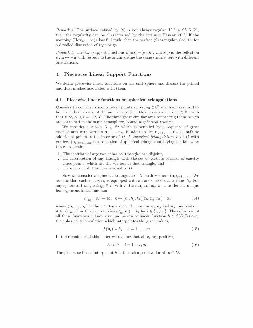
Fig. 5. Quasi–convex polygons as offsets of convex polygons.

we choose one of the two possible unit normal vectors ni lying in T. The polygonalong with the unit normals is then called an oriented polygon. At each vertexqi we consider the convex cone

Ci = λni−1 + µni mod v : λ ≥ 0, µ > 0, i = 1, . . . , v. (22)

The oriented polygon is said to be quasi–convex if i 6= j implies Ci ∩ Cj = ∅.

According to this definition, a quasi–convex polygon is characterized by thefact that the oriented unit normals trace the unit circle exactly once. Any con-vex polygon, where all edges are oriented by choosing either outward or inwardpointing normals, is also quasi–convex. A general quasi–convex polygon is ob-tained as an offset of a convex one, where all edges are simply translated by acertain signed distance, according to the given normals.

Remark 5. If T is the plane R2, then an oriented polygon can be described by a

piecewise linear support function on the unit circle S1. The edges and verticesof the polygon correspond to the nodes and to the linear pieces of this function,respectively.

4.4 The primal mesh

Each triangle ijk ∈ T has an associated linear support function h∗

ijk whichdefines a triangular facet Pijk of the dual mesh. By applying the polarity to theplane spanned by this facet, we obtain the corresponding point

pijk = ((hi, hj , hk)(ni,nj ,nk)−1)⊤ (23)

of the primal mesh.For any inner vertex ni ∈ intD of the spherical triangulation we consider the

star of this vertex, i.e., the set of triangles sharing this vertex,

Si = ijk ∈ T : j, k ∈ 1, . . . , m. (24)

(a) (b) (c) (d) (e)

Fig. 6. Stars of vertices of the dual mesh and the associated quasi–convex polygons ofthe primal mesh: convex, simple (a); non–convex, simple (b,c); non–convex, non–simple(d,e).

Each triangle ijk corresponds to a point pijk. All these points lie in the plane

Ti = x ∈ R3 : x · ni = hi, (25)

which is obtained by applying the polarity to the vertex pi. By connecting points,where the corresponding triangles have a common edge, we obtain a polygon.

Example 2. Five different stars and the associated planar polygons are shownin Fig. 6. If the vertex is convex, then the associated polygon is also convex.Otherwise, non–convex and even non–simple polygons may be obtained.

Proposition 2. The primal mesh p associated with the piecewise linear sup-port function h ∈ C(D, R) satisfying (15) over the given spherical triangulation Tof D with vertices (ni)i=1,...,m is the set of (not–necessarily simple) quasi–convexplanar polygons with vertices pijk . These polygons will be called the facets of p.For each inner vertex ni of the triangulation, the star of this vertex defines oneof these polygons, and this polygon lies in the plane Ti.

Proof. Without loss of generality we consider the star of the vertex ni = (0, 0, 1)⊤.We consider a certain neighborhood of the corresponding vertex ti = (1/hi)ni ofthe dual mesh. Since it is star–shaped with respect to the origin, the dual meshcan be represented as

(1 − t)

00

1/hi

+ t

cosφsinφz(φ)

, φ ∈ R, t ∈ [0, ǫ] (26)

where the 2π–periodic continuous function z(φ) is piecewise smooth (in the inte-riors of the triangles Pijk). It has jumps in the first derivatives exactly in those

directions that correspond to edges shared by neighboring triangles of the dualmesh.

On the one hand, by applying the polarity to the planes spanned by thetriangles Pijk we obtain the vertices of the quasi–convex polygon in the plane Ti.On the other hand, by applying the polarity to the parameter lines φ =constantin (26) we obtain oriented lines with the normal vector (cosφ, sin φ, 0)⊤ in thisplane. In particular, the lines which correspond to shared edges of neighboringtriangular facets of the dual mesh correspond to the edges of the quasi–convexpolygon. The remaining lines support that polygon at its vertices. ⊓⊔

A simple polygon of the primal mesh will be said to be regular. A primal meshwith only simple polygons will also be said to be regular. We discuss criteriawhich guarantee regularity.

Lemma 1. Let ti be a an inner v-vertex of the dual mesh P and tj(1), . . . , tj(v)

be the neighboring vertices in counterclockwise order. We assume that no twoedges meeting at ti are linearly dependent.

The quasi–convex polygon which corresponds to the star of ti has a self–intersection if and only if there exists two points tj(k), tj(l) such that the twopoints tj(k−1), tj(k+1) are on the same side of the plane spanned by tj(k), tj(l)

and ti, and also the two points tj(l−1), tj(l+1) are on the same side of this plane.

Proof. Applying the polarity to the plane spanned by tj(k), tj(l) and ti gives theintersection point of the polygon. ⊓⊔

In particular, if the dual mesh is convex, then all facets of the primal meshare also convex and therefore regular.

4.5 Examples

We use spherical triangulations whose vertices are obtained by applying uniformrefinement steps (where each triangle is split into four triangles by halving theedges) to a icosahedron, and projection onto the unit sphere after each refinementstep. This gives dual meshes which are adapted to the curvature of the mesh;more facets are used in regions with higher curvature.

Example 3. We consider an ellipsoid with three different diameters and its dualsurface, which is again an ellipsoid. The vertices ni of the spherical triangulationwere obtained by applying two steps of refinement to a regular icosahedron. Thethree symmetry planes of the ellipsoid were aligned with symmetry planes of theicosahedron.

We considered only the upper half of the ellipsoid. The piecewise linear in-terpolant to the support function of the ellipsoid defines a dual mesh with 90vertices. This dual mesh is convex, hence the 90 facets of the associated primalmesh do not have any self–intersections. A physical model of this mesh is shownin Figure 7.

Fig. 7. Example 3. Convex mesh with piecewise linear support function which approx-imates a segment of an ellipsoid. The mesh consists of 90 facets.

Most facets of the primal mesh have 6 vertices, and most vertices of theprimal mesh have valency 3. In some cases, the edges of the facets are veryshort, and two of these vertices are virtually identical, leading to a vertex withvalency 4. This situation corresponds to two neighboring triangles of the dualmesh which are almost coplanar.

Example 4. We consider a one–sheeted hyperboloid with three different diame-ters and its dual surface, which is again a one–sheeted hyperboloid. Similarly tothe previous example. the vertices ni of the spherical triangulation were obtainedby applying three steps of refinement (where each triangle is split into four trian-gles by halving the edges) to a regular icosahedron. The three symmetry planesof the hyperboloid were aligned with symmetry planes of the icosahedron.

We considered a segment of the upper half of the hyperboloid, which isbounded by two vertical planes. The piecewise linear interpolant to the sup-port function of the hyperboloid defines a dual mesh with 169 vertices. Thisdual mesh is non–convex, but nevertheless each vertex defines a regular facet ofthe primal mesh. A physical model of this mesh is shown in Figure 8.

As in the previous example, most of the 169 facets of the primal mesh have6 vertices, and most vertices of the primal mesh have valency 3.

5 Tangent meshes

We discuss the construction of meshes whose facets lie in the tangent planes of agiven surface. For a spherical triangulation with vertices n1, . . . ,nk and a given(smooth) surface with support function h(n), one can construct piecewise linearsupport function by choosing hi = h(ni) in (14), i.e., by sampling values of thesupport function of the given surface. However, we have to ensure the regularityof the corresponding primal mesh.

Fig. 8. Example 4. Non–convex mesh with piecewise linear support function whichapproximates a segment of a one–sheeted hyperboloid. The mesh has 169 facets.

Two approaches will be presented. In the first approach, we consider a se-quence of spherical triangulations with decreasing size of the triangles. Theycorrespond to triangular (dual) meshes approximating the dual surface with in-creasing level of accuracy. Here we analyze the limit shapes of the facets of theprimal mesh. This approach is particularly well suited for primal surfaces withonly hyperbolic points, see Sections 5.1 and 5.2.

The second approach is restricted to primal surfaces with only elliptic points.In this case a suitable dual mesh can be found via convex hull computation, seeSection 5.3.

5.1 Asymptotic behavior of the vertices of the primal mesh

We assume that we can generate an increasingly fine triangulation (the dualmesh) of the dual surface, which depends on some step-size h. In order to studythe limit shape of the facets of the corresponding primal mesh when h tends tozero, we consider the following situation.

We consider the dual surface P in the vicinity of one of its points P0 =P(u0, v0). Consider two C3 curve segments a(h), b(h), h ∈ (−ǫ, ǫ), which lie onP and satisfy a(0) = b(0) = P0 and a′ × b′ = λn0, λ > 0, where n0 is thenormal of the dual surface at P0 and the prime ′ denotes the first derivativewith respect to h at h = 0. Let Q(h) be the plane spanned by P0,a(h),b(h) andq(h) its image under the polarity with respect to the unit sphere tangent to P

at P0 and having n0 for outer normal.

After a suitable translation, the sphere can be chosen as the unit sphere S2

centered at the origin, as described in Section 3.1. The plane Q(h) is well–definedfor all h 6= 0, provided that ǫ is sufficiently small.

The limit behavior of q(h) for decreasing step-size h is described in thefollowing result.

Lemma 2. The point q(h) lies in the tangent plane to P at P0. It satisfies

limh→0

q(h) = P0 and q′ =|b′|2 κba

′ − |a′|2 κab′

2(a′ × b′) · n0× n0, (27)

where κa and κb are normal curvatures of the tangent directions a′ and b′,respectively.

Proof. The two given curves have Taylor expansions of the form

a(h) = P0 + a′h +1

2(|a′|2 κan0 + ta)h

2 + O(h3) (28)

b(h) = P0 + b′h +1

2(|b′|2 κbn0 + tb)h2 + O(h3), (29)

where the vectors ta, ta are perpendicular to n0. We compute a normal to theplane Q(h)

NQ(h) = (a(h) − P0) × (b(h) − P0) =

= (a′ × b′)[

h2 + ch3]

+ 12 (|b′|2 κba

′ − |a′|2 κab′) × n0h

3 + O(h4),(30)

where

c =(a′ × tb − b′ × ta) · (a′ × b′)

2|a′ × b′|2 . (31)

Since the plane Q(h) contains the point P0 = n0, it has the equation

x ·NQ(h) = n0 · NQ(h) = (a′ × b′) · n0

[

h2 + ch3]

+ O(h4). (32)

Hence, the corresponding dual point is

q(h) =NQ(h)

(a′ × b′) · n0 [h2 + ch3] + O(h4)=

= P0 +|b′|2 κba

′ − |a′|2 κab′

2(a′ × b′) · n0× n0h + O(h2).

(33)

Though the calculation of q(h) is not valid for h = 0, the function q can beextended to a C2 function by letting q(0) = P0. ⊓⊔

Using a regular parameterization P = P(u, v) of the dual surface, we canexpress q′ with the help of the second fundamental form.

Lemma 3. Assume that Pu(u0, v0) × Pv(u0, v0) is a positive multiple of n0,where Pu, Pv denote the first derivatives of P with respect to the parameters. IfP0 = P(u0, v0), a(h) = P(ua(h), va(h)) and b(h) = P(ub(h), vb(h)) then

q′ = P⊥

u

L(

u′au′

b2 − u′

a2u′

b

)

+ 2Mu′

bu′a (v′b − v′a) + N

(

u′av′b

2 − v′a2u′

b

)

2(u′av

′

b − v′au′

b)+

+P⊥

v

L(

v′au′

b2 − u′

a2v′b

)

+ 2Mv′av′b (u′

b − u′

a) + N(

v′b2v′a − v′bv

′

a2)

2(u′av′b − v′au′

b)

(34)

where L, M, N are the coefficients of the second fundamental form at P0, and

P⊥

u =1√

EF − G2

∂P

du

∣

∣

∣

∣

u0,v0

× n0, P⊥

v =1√

EF − G2

∂P

dv

∣

∣

∣

∣

u0,v0

× n0, (35)

where E, F, G are the coefficients of the first fundamental form at P0.

This fact can now be verified by a direct computation.

5.2 Asymptotic behavior of the facets of the dual mesh

Eq. (34) gives the leading term of q(h) with respect to the basis P⊥

u , P⊥

v . Weuse it to define the limit shape of a facet.

Definition 2. Consider the dual surface P(u, v), which is assumed to be regu-lar and C3 in the vicinity of P(0, 0). Let (u1, v2), (u2, v2), . . . , (un, vn) be theparameter values of the star of the vertex P(0, 0). We define the vertices of thelimit shape of the primal facet by applying the expression (34) to the con-secutive pairs of dual vertices. More precisely, the limit position of the vertex ofthe primal facet associated with the triangle with vertices

P(ui, vi), P(u(i mod n)+1, v(i modn)+1), P(0, 0), i = 1, . . . , n, (36)

is found by substituting

u′

a = ui, v′a = vi, u′

b = u(i modn)+1, and v′b = v(i modn)+1 (37)

in the right–hand side of (34), and the limit shape is obtained by connectingconsecutive pairs of limit vertices.

The geometrical meaning of the limit shape of the primal polygon is describedin the following result.

Proposition 3. We consider the primal facet associated with the star of thedual mesh with apex P(0, 0) and vertices P(h ui, h vi), i = 1, . . . , n. As h → 0,the shape of the primal facet tends to the corresponding limit shape.

The proof is a direct consequence of Lemma 3.By using a regular triangular mesh with edge–length h in the parameter

domain of the dual surface, one might expect to obtain regular facets of theprimal mesh as h tends to zero. However, this is not the case as shown by thefollowing example.

Example 5. Consider the following elliptic dual surface

(u, v, 1.34u2 + 1.89uv + 0.72v2), (38)

and choose the parameters (ui, vi) as the vertices of a regular hexagon in theu, v-plane inscribed in the unit circle. Figure 9 shows the regular polygon (thin)with its limit primal polygon (thick), which is not simple.

In order to obtain a regular primal mesh approximating a patch of of ahyperbolic surface, we propose the following

–3

–2

–1

0

1

2

3

–3 –2 –1 0 1 2 3

Fig. 9. The limit shape (thick polygon) associated with the star defined by the regularhexagon for the surface (38).

Algorithm 1

Input: Smooth dual hyperbolic surface P with a C3 curve α(t) lying on it, andstep size h. The curve α(t) must not touch the asymptotic lines of the dualsurface.Output: Triangular (dual) mesh of the dual surface and associated primal mesh.

1. Compute the diagonal points [n, n] := α(nt).2. Compute the general grid points [m, n] defined as intersection of the ‘vertical’

asymptotic line through [m, m] and the ‘horizontal’ asymptotic line through[n, n]. Here, the notions ‘vertical’ and ‘horizontal’ are used to distinguishbetween the two different families of asymptotic lines on the dual surface.

3. Produce the triangular mesh by applying the pattern shown in Figure 10,left.

4. Compute the primal mesh.

Now we can prove that this algorithm produces a sensible output, at least ash tends to zero.

Theorem 1. If the step size h is sufficiently small, then the algorithm producesa regular primal mesh.

Proof. There exists a unique parameterization P(u, v) of the dual surface suchthat the the parametric directions are the asymptotic lines and α(t) = P(t, t).In this parameterization, the second fundamental form satisfies L = N = 0and we can compute the limit shape of the primal facets associated with thestars of the dual mesh (indicated by the grey hexagons in Fig. 10, left). In thisparameterization we apply directly the formula (34). Note that L = N = 0.Setting M = 1 we obtain the regular limit shape shown in Figure 10, right.

Different values of M only scale the limit shape. Note that this shape corre-sponds to the polarity with respect to a unit sphere which is tangent to the dual

m

n

–2

–1

0

1

2

–2 –1 0 1 2

Fig. 10. Left: Pattern for producing the dual mesh from the dual surface. The verticaland horizontal lines represent the grid of asymptotic lines, while the circles indicatewhich points should be sampled. Right: The limit shape (thick curve) of the star definedby the thin polygon, which corresponds to the hexagons shown in the left figure.

surface at the corresponding vertex. The global polarity π, however, modifiesthis shape by a projective transformation which can be shown to preserve theregularity, provided that the step–size is sufficiently small ⊓⊔

We illustrate this result by two examples.

Example 6. Consider the Enneper surface(

13 (u + v)(2u2 − 8uv + 3 + 2v2), 1

3 (u − v)(2u2 + 8uv + 3 + 2v2), 4uv + 1))

,

where the parameter lines are already the asymptotic lines. The dual surface hasthe parametric representation

P(u, v) =

6(u+v)(8u3v+6u2+8uv3+12uv+6v2−3)

−6(−v+u)(8u3v+6u2+8uv3+12uv+6v2−3)

3(2v2+2u2−1)

(8u3v+6u2+8uv3+12uv+6v2−3)

. (39)

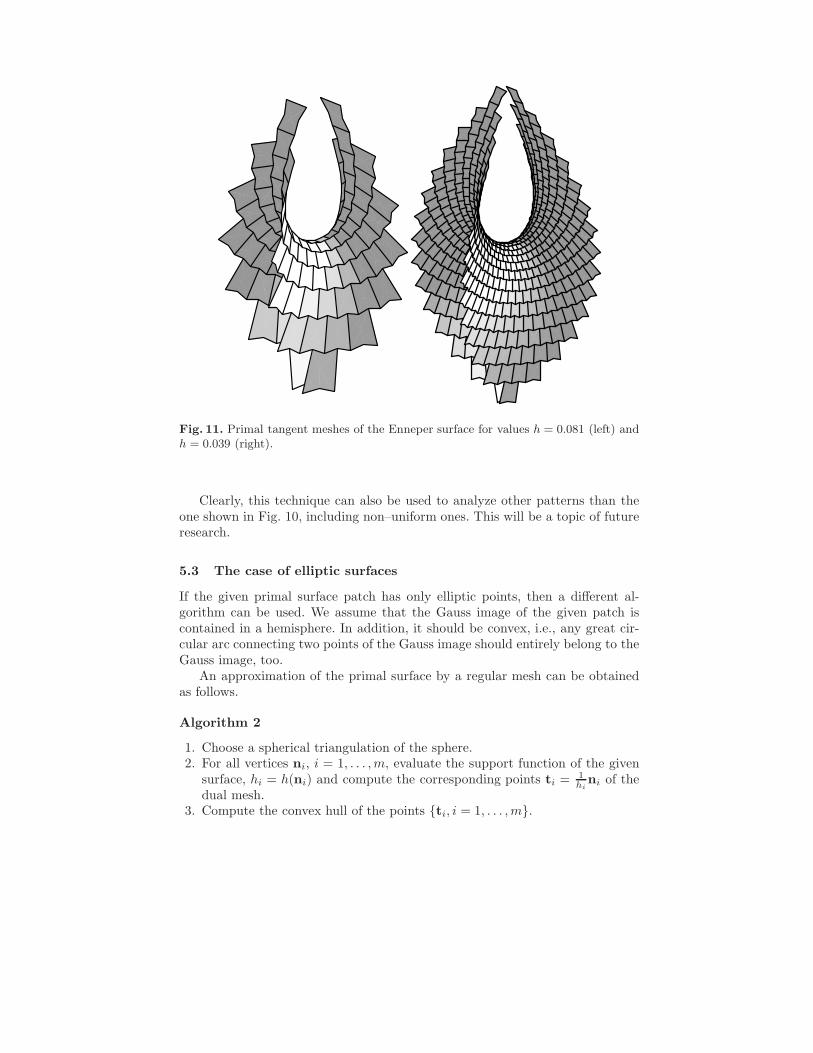
By choosing α(t) = P(t, t) and suitable h we obtain a dual mesh of P and finallya regular primal mesh which approximates the Enneper surface – see Figure 11.

This example is somewhat special, since the asymptotic lines intersect eachother orthogonally (as it is a minimal surface). This is not the case of the secondexample.

Example 7. We consider a segment of a ruled quadric, where the parameter linesare the two families of straight lines on this surface. By applying the algorithmwith three different step-sizes we obtain the primal meshes shown in Fig. 12.

Fig. 11. Primal tangent meshes of the Enneper surface for values h = 0.081 (left) andh = 0.039 (right).

Clearly, this technique can also be used to analyze other patterns than theone shown in Fig. 10, including non–uniform ones. This will be a topic of futureresearch.

5.3 The case of elliptic surfaces

If the given primal surface patch has only elliptic points, then a different al-gorithm can be used. We assume that the Gauss image of the given patch iscontained in a hemisphere. In addition, it should be convex, i.e., any great cir-cular arc connecting two points of the Gauss image should entirely belong to theGauss image, too.

An approximation of the primal surface by a regular mesh can be obtainedas follows.

Algorithm 2

1. Choose a spherical triangulation of the sphere.2. For all vertices ni, i = 1, . . . , m, evaluate the support function of the given

surface, hi = h(ni) and compute the corresponding points ti = 1hi

ni of thedual mesh.

3. Compute the convex hull of the points ti, i = 1, . . . , m.

Fig. 12. Primal tangent meshes of a ruled quadric for three different values of h.

4. The apparent contour of the convex hull, seen from the origin, splits theboundary surface of the convex hull into two meshes. One of them is thesuitable dual mesh; the other one does not have any inner vertices.

Due to the fact that the dual surface of the elliptic point is also elliptic, all verticesof the dual mesh obtained from this algorithm have convex stars. Consequently,all faces of the primal mesh are convex (and therefore simple) polygons.

An example has already been presented in Section 4.5 (Example 3).

6 Conclusion

Based on the use of piecewise linear support functions we discussed dual meshes,which were assumed to be star–shaped with respect to the origin, and the asso-ciated primal meshes. The primal meshes are capable of approximating smoothsurface patches without parabolic points. It should be noted that these meshesapproximate not only the surfaces but also the associated normals. I.e., eachnormal in the Gauss image corresponds to exactly one normal on the primalmesh. This is clearly not the case for general meshes which approximate a givensurface.

As a matter of future work we will use the support function for generatingerror bounds. In the smooth case the maximum distance error is essentiallyequal to the maximum difference between the original support function and itsapproximation. While this is also true for convex primal meshes, the extensionof this result to the non–convex case is still an open problem.

In addition, we plan to discuss the approximation of general support functionsby piecewise linear support functions over a given spherical triangulation, subjectto conditions which guarantee the regularity of the resulting primal mesh. In thecase of elliptic surfaces, this can be formulated as an optimization problem withlinear constraints. In the hyperbolic case, however, non–linear constraints areneeded.

Finally we plan to investigate surfaces with parabolic lines separating ellip-tic and hyperbolic regions. In order to represent these surfaces, multi–valuedpiecewise linear functions will be needed.

Acknowledgment. This research was supported by a grant of the Austrian Sci-ence Fund (FWF, project no. P17387-N12 and SFB F013, subproject 15), byresearch project no. MSM 0021620839 at Charles University, Prague, and by theproject “Facetted glass shells” at the Department of Civil Engineering of DanishTechnical University. The authors wish to thank the reviewers for their usefulcomments. Special thanks go to Bert’s father for building the two models shownin Figures 7 and 8.

References

1. H. Almegaard: The stringer system - a truss model of membrane shells for analysisand design of boundary conditions. International Journal of Space Structures 19

(2004), 1-10.2. T. Bonnesen and W. Fenchel: Theory of convex bodies. BCS Associates, Moscow,

Idaho, 1987.3. M. Bruckner: Vielecke und Vielflache – Theorie und Geschichte, Teubner, Leipzig

1900.4. B. Cutler and E. Whiting: Constrained Planar Remeshing for Architecture, in:

Symposium on Geometry Processing 2006, Poster proceedings (electronic), p. 5,http://sgp2006.sc.unica.it/program/PosterProceedings.pdf.

5. H. Groemer: Geometric Applications of Fourier Series and Spherical Harmonics

Cambridge University Press, Cambridge, 1996.6. P. M. Gruber and J. M. Wills (eds.): Handbook of convex geometry, North–Holland,

Amsterdam, 1993.7. J. Hoschek and D. Lasser: Fundamentals of Computer Aided Geometric Design,

AK Peters, Wellesley Mass., 1996.8. J. Hoschek: Dual Bezier curves and surfaces, in: Surfaces in Computer Aided Geo-

metric Design, R.E. Barnhill and W. Boehm, eds., North Holland, 1983, 147–156.9. H. Kawarahada and K. Sugihara: Dual subdivision: A new class of subdivision

schemes using projective duality, in WSCG’2006 Full paper proceedings, J. Jorgeand V. Skala, eds., University of West Bohemia, Plzen 2006, 9–16.

10. Y. Liu, H. Pottmann, J. Wallner, Y. Yang and W. Wang: Geometric Modeling withConical Meshes and Developable Surfaces. ACM Trans. Graphics 25 (Siggraph2006), 681-689.

11. G. Patane and M. Spagnuolo: Triangle Mesh Duality: Reconstruction and Smooth-ing, in The Mathematics of Surfaces X, M. Wilson and R. Martin, eds., SpringerLNCS 2768, 111–128, Berlin 2003.

12. H. Pottmann and J. Wallner, The focal geometry of circular and conical meshes,Adv. Comput. Math., to appear.

13. L. Ros, K. Sugihara, F. Thomas: Towards shape representation using trihedralmesh projections, The Visual Computer 19 (2003), 139–150.

14. M. Sabin: A Class of Surfaces Closed under Five Important Geometric Operations,Technical report no. VTO/MS/207, British aircraft corporation, 1974, available athttp://www.damtp.cam.ac.uk/user/na/people/Malcolm/vtoms/vtos.html

15. Z. Sır, J. Gravesen and B. Juttler: Curves and surfaces represented by polyno-mial support functions, SFB report no. 2006–36, available at http://www.sfb013.uni-linz.ac.at.

16. E. W. Weisstein: Dual Polyhedron. From MathWorld – A Wolfram Web Resource.http://mathworld.wolfram.com/DualPolyhedron.html

17. M. J. Wenninger: Dual models, Cambridge University Press 1983.