Surveying-I Laboratory Manual · through commercial Pipes ... Non inertial cavitation is the...

Prepared by: Mr. Avijit Paul

Approved by: Dr. Arabinda sharma

Civil Engineering Department

BRCM College of Engg & Technology

Bahal-127 028, Bhiwani

Haryana

2014 Fluid Mechanics-II Laboratory Manual


Prepared By: Avijit Paul - 2 - Approved By: Dr. Arabinda Sharma

Experiment: 1

LIST OF EXPERIMENTS

1. To determine the coefficient of drag by stokes law for

sphere

2. To study the phenomenon of cavitation in pipe flow

3. To determine the critical Reynolds number for flow

through commercial Pipes

4. To determine the coefficient of discharge for flow over a

broad crested weir

5. To study the characteristics of a hydraulic jump

6. To study the scouring phenomenon around a bridge pier

model

7. To study the characteristics of a centrifugal pump

8. To study the momentum characteristics of a impact jet

9. To determine head loss due to various pipe fittings

http://www.brcm.edu.in/college/



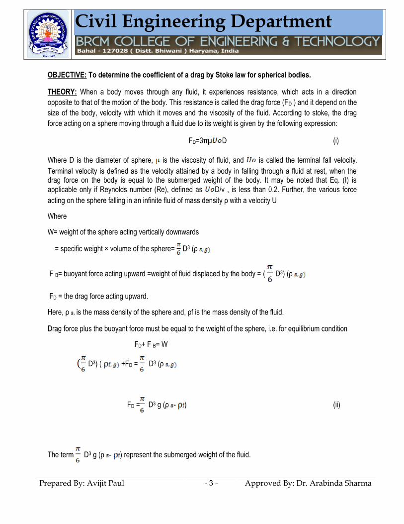
OBJECTIVE: To determine the coefficient of a drag by Stoke law for spherical bodies.

THEORY: When a body moves through any fluid, it experiences resistance, which acts in a direction

opposite to that of the motion of the body. This resistance is called the drag force (FD ) and it depend on the

size of the body, velocity with which it moves and the viscosity of the fluid. According to stoke, the drag

force acting on a sphere moving through a fluid due to its weight is given by the following expression:

FD=3πµ D (i)

Where D is the diameter of sphere, is the viscosity of fluid, and is called the terminal fall velocity.

Terminal velocity is defined as the velocity attained by a body in falling through a fluid at rest, when the drag force on the body is equal to the submerged weight of the body. It may be noted that Eq. (I) is

applicable only if Reynolds number (Re), defined as D/v , is less than 0.2. Further, the various force

acting on the sphere falling in an infinite fluid of mass density ρ with a velocity U

Where

W= weight of the sphere acting vertically downwards

= specific weight × volume of the sphere= D3 (ρ

F B= buoyant force acting upward =weight of fluid displaced by the body = ( D3) (ρ

FD = the drag force acting upward.

Here, ρ is the mass density of the sphere and, ρf is the mass density of the fluid.

Drag force plus the buoyant force must be equal to the weight of the sphere, i.e. for equilibrium condition

FD+ F B= W

D3) ( +FD = D3 (ρ

FD = D3 g (ρ - ) (ii)

The term D3 g (ρ - ) represent the submerged weight of the fluid.




Equating Eqs.(i) and (ii) , we get

3πµ D= D3 g (ρ - )

= 18

2Dg (ρ - ) =

18

2D (ρ - ) (iii)

Equation (iii) is the required expression for terminal velocity.

Also, drag force acting on the body moving in a fluid of density is given by the following expression.

FD= CDA2

2

0Uf (iv)

Where CD is the coefficient of drag and A is the projected area of the object on a plane normal to the

direction of flow. For a sphere, projected area A= 4

2D . CD = , where = (v)

Thus, coefficient of a drag CD varies with Reynolds number.

Experiment has shown that Eq.(v) hold good for Re 0.2,and the sphere is falling in an infinite fluid. If the

fluid is not infinite in extent but is confined with a container (finite dimension), then the resistance to motion is increased , and in such a case the modified value of drag coefficient, as given by the following expression, should be used :

CD = (1+2.1 ) (vi)

Where D1 is the smallest lateral dimension of the container and D is the diameter of the sphere.

Also the observed fall velocity is corrected in Eq.(iii) by using the following expression in order to get all

the fall velocity corresponding to infinite fluid medium:

Corrected velocity, = (1+2.4 ) (vii)

Where D1 is the diameter of container.

EXPERIMENTAL SET- The set up consists of a transparent vertical cylinder. A hopper with a valve is

provided at the bottom of the cylinder to collect the sphere. The cylinder is supported by four vertical posts




and fixed to MS table. A vertical scale is fixed on the surface of a cylinder. The cylinder is filled with highly

viscous fluid such as glycerin.

PROCEDURE: 1. Measure the diameters of sphere and note down their materials.

2. Determine the mass of the sphere on electronic balance.

3. Mark two line on the cylinder for measurement of the vertical distance (L) for the determination of

terminal velocity. The upper line should be at a depth of 100mm or more from the free surface so that the

terminal velocity is achived.

4. Hold the sphere with a finger and a thumb and bring it with up to the fluid level. Leave the sphere

gently(wet the sphere before dropping it ).

5. Note down the time taken by the sphere in falling through distance L.

6. Repeat steps (4) and (5) for other diameter of sphere (Set1).

7. Repeat step (4) to (6) For sphere of other material (Set2)

OBSERVATIONS AND CALCULATIONS:

Liquid in the cylinder =

Mass density of liquid =

Kinetic viscosity of liquid at T ,v=

Diameter of cylinder, D1 =

Distance of fall,L=

Material of sphere




Run No. Diameter

D

Projected

area, A

Mass

density,

ρ

FD CD by

eq (iv)

Re= CD by eq

(v)

1.

2.

3.

GRAPH: Plot CD versus Re as abscissa on an ordinary graph paper.

EXPERIMENT NO - 2




OBJECTIVE: To study the phenomenon of cavitation in pipe flow

INTRODUCTION AND THEORY:

Cavitation is the formation and then immediate implosion of cavities in liquid – i.e. small liquid-free zones

("bubbles") – that are the consequence of forces acting upon the liquid. It usually occurs when a liquid is

subjected to rapid changes of pressure that cause the formation of cavities where the pressure is relatively

low.

Cavitation is a significant cause of wear in some engineering contexts. When entering high pressure areas,

cavitation bubbles that implode on a metal surface cause cyclic stress. These results in surface fatigue of

the metal causing a type of wear also called "cavitation". The most common examples of this kind of wear

are pump impellers and bends when a sudden change in the direction of liquid occurs. Cavitation is usually

divided into two classes of behavior: inertial (or transient) cavitation and non-inertial cavitation.

Inertial cavitation is the process where a void or bubble in a liquid rapidly collapses, producing a shock

wave. In man-made objects, it can occur in control valves, pumps, propellers and impellers.

Non inertial cavitation is the process in which a bubble in a fluid is forced to oscillate in size or shape due to

some form of energy input, such as an acoustic field. Such cavitation is often employed in ultrasonic

cleaning baths and can also be observed in pumps, propellers, etc.

Since the shock waves formed by cavitation are strong enough to significantly damage moving parts,

cavitation is usually an undesirable phenomenon. It is specifically avoided in the design of machines such

as turbines or propellers, and eliminating cavitation is a major field in the study of fluid dynamics.

Hydrodynamic cavitation describes the process of vaporization, bubble generation and bubble implosion

which occurs in a flowing liquid as a result of a decrease and subsequent increase in pressure. Cavitation

will only occur if the pressure declines to some point below the saturated vapor pressure of the liquid. In

pipe systems, cavitation typically occurs either as the result of an increase in the kinetic energy (through an

area constriction) or an increase in the pipe elevation.

Hydrodynamic cavitation can be produced by passing a liquid through a constricted channel at a specific

velocity or by mechanical rotation through a liquid. In the case of the constricted channel and based on the

specific (or unique) geometry of the system, the combination of pressure and kinetic energy can be created

when the hydrodynamic cavitation cavern downstream of the local constriction generating high energy

cavitation bubbles.

The process of bubble generation, subsequent growth and collapse of the cavitation bubbles results in very

high energy densities, resulting in very high temperatures and pressures at the surface of the bubbles for a

very short time. The overall liquid medium environment, therefore, remains at ambient conditions. When




uncontrolled, cavitation is damaging; however, by controlling the flow of the cavitation the power is

harnessed and non-destructive. Controlled cavitation can be used to enhance chemical reactions or

propagate certain unexpected reactions because free radicals are generated in the process due to

disassociation of vapors trapped in the cavitating bubbles.

Cavitation is, in many cases, an undesirable occurrence. In devices such as propellers and pumps,

cavitation causes a great deal of noise, damage to components, vibrations, and a loss of efficiency. When

the cavitation bubbles collapse, they force energetic liquid into very small volumes, thereby creating spots

of high temperature and emitting shock waves, the latter of which are a source of noise. The noise created

by cavitation is a particular problem for military submarines, as it increases the chances of being detected

by passive sonar. Although the collapse of a cavity is a relatively low-energy event, highly localized

collapses can erode metals, such as steel, over time. The pitting caused by the collapse of cavities

produces great wear on components and can dramatically shorten a propeller or pump's lifetime. After a

surface is initially affected by cavitation, it tends to erode at an accelerating pace. The cavitation pits

increase the turbulence of the fluid flow and create crevasses that act as nucleation sites for additional

cavitation bubbles. The pits also increase the components' surface area and leave behind residual

stresses. This makes the surface more prone to stress corrosion.

Experiment: 3

OBJECTIVE: To determine the critical Reynolds number for flow through commercial pipes.




THEORY: Depending upon the relative magnitude of inertia and viscous forces, the flow of fluid in a pipe

may be either laminar or turbulent. In laminar flow, viscous effects are more predominant then the inertial

effects. But when the velocity of flow is increased, the flow become turbulent as shear and normal stress

are added to the flow. A convenient measure of the two types of flow is Reynolds number, denoted by Re.

It is defined as the ratio of inertia force to the viscous force and is given by the expression VD/v, where V is

the average velocity of flow, D diameter of pipe, and v is the kinematic viscosity of the fluid. For pipes, if Re

2000, flow is laminar and for Re 4000 the flow is turbulent. For Re lying between 2000 4000, the flow

is in the transition stat, which refer to the change of flow laminar to turbulent occurring in some limited

region of flow.

Osborne Reynolds was the first who demonstrated the existence of the two types of flow, viz. laminar and

turbulent, experimentally. Reynolds injected dye as filament at the centre of a transparent tube and studied

its behavior. He observed that at low flow velocities, the dye remained in the form of straight and stable

filament so steadily that it hardly seemed to be in motion. This corresponds to laminar flow conditions. With

the increase in velocity of flow, a critical state was reached at which the filament of dye showed signs of

irregularities and began to wavers. This show that the flow is no longer laminar but in transitional state.

With further increase in velocity of flow, the dye completely diffused over the cross section of the tube and

mixed with water. This corresponds to the turbulent flow conditions.

The velocity at which the flow changes from laminar to turbulent is called the upper critical velocity, and the

corresponding Reynolds number as the upper critical Reynolds number. The velocity at which the flow

changes back from turbulent to laminar is called the lower critical velocity, and the corresponding Reynolds

number as the lower critical Reynolds number. The upper critical Reynolds number is not a fixed quantity

as it depend upon a number of factors such as initial disturbance to flow, the shape of entry to the tube, etc.

On the other hand, the lower critical Reynolds number is well established and its value is usually about

2000.

EXPERIMENTAL SET UP:




The set up consists of a constant head supply tank mounted on a steel plate and placed on MS stand. A

Perspex tube is attached to the tank to visualize the different flow conditions. The tank has the provision for

supplying dye through a needle at the centre of the tube in the form of a jet. The entry of water in perspex

tube is through an elliptical bell mouth entrance so as to have a smooth entry to the flow. Water is supplied

to the tank through an inlet valve provided in the supply pipeline. A regulating valve is provided on the

downstream side of the tube to regulate the flow gradually. A collecting tank is provided to measure the

discharge. Alternatively, smaller discharge can be measured in the cylinder.

PROCEDURE:

1. Open the inlet valve slightly and maintain constant head in the supply tank by adjusting the inflow. Let

the flow become steady.

2. Inject dye slowly and study its characteristic/behavior.

3. Measure discharge.

4. Increase the discharge slightly by opening the outlet valve. Again maintain constant head in the supply

tank.

5. Repeat the above step for different discharges till dye gets completely diffused over the cross section of

the tube.

(Encircle the reading for which the dye filament wavers for the first time near the outlet end of the

tube.)

6. Repeat the experiment with decreasing rate of flow and encircle the reading for which the dye filament

wavers for the last time near the outlet end of the tube, as the flow changes back from laminar to turbulent.

OBSERVATIONS AND CALCULATIONS

Diameter of Perspex tube, d =




Area of conduit ,a =

Temperature of water, T =

Kinematic viscosity of water at T =

Area of collecting tank, A =

Increasing discharge

Run No. Discharge, Q V = Re = Characteristic of dye Remarks

1.

2.

3.

Decreasing discharge

Run No. Discharge, Q V = Re = Characteristic of dye Remarks

1.

2.

3.

EXPERIMENT NO. - 4

OBJECTIVE: To determine the coefficient of discharge of a Broad crested weir.




EQUIPMENT USED:

1) A channel or flume to provide a flow passage.

2) A broad crested weir.

3) Hook-gauge to measure the head over the crest over the crest of weir.

4) A collecting tank to fit with a pyrometer, to the discharge over the weir and to find out actual discharge.

5) Stop watch to note the time of collection of water for a known rise of water level in the collecting tank.

6) Meter scale to measure the internal plan dimensions of the collecting tank.

PROCEDURE:

Start the experiment by pressing start button with default values of length of the collecting -tank, width of

the collecting, pause the experiment after few cycles and note the observation.

Observation1:

1) Open the control valve and allow the water level to rise up to the skill level of the weir.

2) Adjust the tip of the hook gauge such that it coincides with water surface and note the

reading on hook gauge scale as h1 on u/s.

Observation2:

1) Operate the control valve such that water flows over the weir to some height.

2) Again adjust the tip of the hook gauge such that it coincides with water surface and note the water level

by means of hook gauge as h2.

Observation3:

1) Note the time required for known rise of water level.

2) Keeping the length and width of the collecting tank as default values repeat the experiment by adjusting

flow of water and hook gauge.

Calculation:

Theoretical discharge, Qt = 1.705 L H3/2 in m3/sec

Where,




L = Length of the weir measured parallel to width of channel in meters

H = Constant head over the crest on the upstream of channel in meters.

H = (h2-h1).

Actual discharge ,Q = Internal plan area of collecting tank x rise in collecting tank/ time of

collection (t) in m3/sec.

Internal plan area of the tank, A = L x B =

Actual discharge, Qa= A x Ht =

T = Time taken for rise of 10cms,

H = Rise of water (10cms)

Then, Co-efficient of discharge Cd = Qa/Qt =

Graph:

Draw a graph between Qa and H3/2 taking H3/2 on the x-axis.

EXPERIMENT NO - 5

OBJECTIVE: To study the characteristics of a hydraulic jump on a horizontal floor and sloping

glacis including friction blocks.

THEORY: Hydraulic jump, also known as a standing wave, is the sudden rise of water level that takes

place due to the transformation of unstable (super critical) flow to stable (sub critical) flow. Hydraulic jump




occurs whenever the depth of flow is less then the critical depth. The flow situations where the hydraulic

jump may occur are: The channel width is suddenly increased or decreased, steep channel bottom slope

suddenly change to a flat slope, flow below a sluice, flow at the foot of a spillway, etc.

The flow in a hydraulic jump is rapidly varied and is accompanied by large scale turbulences, in which a

portion of the energy possessed by the flowing water gets dissipated as heat energy. If this energy is not

allowed to dissipate, it may cause damages to downstream protection work or natural erodible bed of the

channel, causing deep scour and sometime even failure of the structure constructed on the channel. The

phenomenon of hydraulic jump is used in the design of hydraulic structure as a mean of energy dissipation

device. Consider hydraulic jump formation in a rectangular channel of unit width, take two section and

immediately before and after the formation of jump. The depth before jump at (say y1) is called initial depth

or pre- jump. After the jump at y2 is called sequent depth or post- jump depth.

Hydraulic Jump

The momentum equation for hydraulic jump in rectangular channel and can be expressed as

= or = (i)

Fr1 = incoming Froude s number, i.e. Froude s number just before jump formation.

Fr2 = outgoing Froude s number, i.e. Froude s number just before jump formation.

Fr1 and Fr2 can be written as




Fr1 = and Fr2 = (ii)

Specific energy before jump, E1 = y1+

Specific energy after jump , E2 =

Therefore, loss of energy

= (E1 E2)

Loss of energy can also be expressed as

= (iii)

The height of the jump (hj) is defined as the difference between the depth after and before the jump, i.e.

hj = (y2-y1) (iv)

Length of the jump (Li)

Li= 7hj (v)

EXPERIMENTAL SET UP:

The set up consists of a recirculating and tilting rectangular flume. The sidewall of the flume are made of a

glass and held between vertical angle iron posts fitted to a steel bottom. The flume has bell shaped

entrance to minimize the separation of flow; two honey comb wall at the inlet to ensure uniform flow and a




sluice gate. The inflow of water in the channel is controlled by using a sluice gate provided at the entrance.

A tail gate is provided at the downstream end of the flume. The flume has a two circular rail at top for

positioning the pointer gauges on wooden platforms and trolleys. Water is supplied to the flume through a

supply valve (delivery valve ) and a venturimeter are provided in the supply pipe for regulating and

measuring the discharge, respectively.

PROCEDURE:

1. Start the pump and open the delivery valve gradually.

2. Adjust the delivery valve, sluice gate and the tailgate so that there forms stable hydraulic jumps in the

flume.

3. Measure water depth at the pre jump section and the post jump section.

4. Measure discharge by using venturimeter.

5. Repeat step (2) and (4) for other discharges by regulating the supply.

OBSERVATIONS AND CAMPUTATIONS:

Width of flume, B =

Pointer gauge reading at bed , y0 =

Run No. Discharge, q y2/y1 Fr1 y2/y1 hj Lj E

1.

2.




3.

GRAPH: 1 Plot ( y2/y1 ) versus Fr1 on an ordinary graph paper. On the same plot, draw a line represented

by Eq. (IV) and note the scatter of the observed data.

2. Plot a graph between hj and Fr1.

3. Plot a graph between E AND Fr1.

EXPERIMENT NO - 6

OBJECTIVE: To study the scouring phenomenon around a bridge pier model

INTRODUCTION AND THEORY:-

Bridge scouring is the removal of sediment such as sand and rocks from around bridge abutments or

piers. Scour, caused by swiftly moving water, can scoop out scour holes, compromising the integrity of a




structure. Bridge scour is one of the three main causes of bridge failure. It has been estimated that 60% of

all bridge failures result from scour and other hydraulic related causes.

Water normally flows faster around piers and abutments making them susceptible to local scour. At bridge

openings, contraction scour can occur when water accelerates as it flows through an opening that is

narrower than the channel upstream from the bridge. Degradation scour occurs both upstream and

downstream from a bridge over large areas. Over long periods of time, this can result in lowering of the

stream bed.

Stream channel instability resulting in river erosion and changing angles-of-attack can contribute to bridge

scour. Debris can also have a substantial impact on bridge scour in several ways. A build-up of material

can reduce the size of the waterway under a bridge causing contraction scour in the channel. A build-up of

debris on the abutment can increase the obstruction area and increase local scour. Debris can deflect the

water flow, changing the angle of attack, increasing local scour. Debris might also shift the entire channel

around the bridge causing increased water flow and scour in another location. During flooding, although the

foundations of a bridge might not suffer damage, the fill behind abutments may scour. This type of damage

typically occurs with single-span bridges with vertical wall abutments.

The examination process is normally conducted by hydrologists and hydrologic technicians, and involves a

review of historical engineering information about the bridge, followed by a visual inspection. Information is

recorded about the type of rock or sediment carried by the river, and the angle at which the river flows

toward and away from the bridge. The area under the bridge is also inspected for holes and other evidence

of scour. Bridge examination begins by office investigation. The history of the bridge and any previous

scour related problems should be notified. Once a bridge is recognized as a potential scour bridge, it will

proceed to further evaluation includes field review, scour vulnerability analysis and prioritize. Bridges will

also be rated in different categories and prioritize for scour risk. Future implementation of scour

countermeasures includes monitoring plans, inspections after flood events, and procedures for closing

bridges if necessary. Alternatively, sensing technologies are also being put in place for scour assessment.

The scour-sensing level can be classified into three levels: general bridge inspection, collecting limited data

and collecting detailed data. There are three different types of scour-monitoring systems: fixed, portable

and geophysical positioning. Each system can help to detect scour damage in an effort to avoid bridge

failure, thus increase public safety.

Bend way weirs, spurs and guide banks can help to align the upstream flow while riprap, gabions,

articulated concrete blocks and grout filled mattresses can mechanically stabilize the pier and abutment

slopes. Riprap remains the most common countermeasure used to prevent scour at bridge abutments. A

number of physical additions to the abutments of bridges can help prevent scour, such as the installation of

gabions and stone pitching upstream from the foundation. The addition of sheet piles or interlocking

prefabricated concrete blocks can also offer protection. These countermeasures do not change the

scouring flow and are temporary since the components are known to move or be washed away in a flood.




Trapezoidal-shaped channels through a bridge can significantly decrease local scour depths compared to

vertical wall abutments, as they provide a smoother transition through a bridge opening. This eliminates

abrupt corners that cause turbulent areas. Spur dikes, barbs, groynes, and vanes are river training

structures that change stream hydraulics to mitigate undesirable erosion or deposits. They are usually used

on unstable stream channels to help redirect stream flow to more desirable locations through the bridge.

The insertion of piles or deeper footings is also used to help strengthen bridges.

Experiment: 7

OBJECTIVE: To study the characteristics of a centrifugal pump

THEORY: A pump is a device which converts mechanical energy into hydraulic energy.

This hydraulic energy is in the form of pressure energy of the liquid, which is subsequently converted into

potential energy as the liquid is lifted from a lower elevation to higher elevation.

Centrifugal pumps fall under the category of roto dynamic pumps that have a rotating element, called

impeller, through which the angular momentum of the liquid changes. The basic principle on which a

centrifugal pumps work is that when a certain of liquid is made to rotate by a an external force, a centrifugal




head is imparted to the liquid. Due to this action, pressure and velocity of liquid increase throughout the

liquid mass (increase in pressure = V 2/ 2g=ω2r2/2g, i.e. it is proportional to the square of angular velocity).

In addition to the centrifugal action as the liquid passes through the revolving impeller, its angular

momentum changes, this also results in increasing the pressure of liquid.

A centrifugal pump is usually designed to work at a particular head, discharge and speed.However, it may

be required to run the pump at the condition different from those for which it is designed. The behavior of

the pump under different condition can be predicted by conducting tests and obtaining the performance

characteristics curves (performance characteristics refer to the graphical representation of variation in

head, power and efficiency of pump drawn to a common base line of flow rate).

The operating characteristics curves are obtained by first running the pump at the designed speed but the

discharge is varied by the mean of delivery valve, whereas in the main characteristics curves, the speed of

the pump is varied and for each speed discharge itself get varied.

EXPERIMENTAL SET UP: The set up consists of closed circuit flow of water in which a centrifugal is

connected to a DC motor. The pressure gauge are provided on the delivery and suction pipe for the

measurement of delivery head and suction head, respectively. A valve is provided on the delivery pipe for

regulating the discharge. The lower end of the suction pipe is fitted with a strainer and a foot valve. The

strainer is provided to keep the debris away from the pump and a foot valve is a non- return or one way

type of valve which opens only in the upward direction, i.e. it will be not allow the liquid to move downwards

back to the sump. A variable speed motor drive is provided for regulating the speed. A tachometer is

provided for measuring the revolutions of the motor. A swinging arm field field dynamometer is connected

on the motor for measurement of load on the motor. A measuring tank is provided for measuring the

discharge through the pump. The water from the pump is discharged into the collecting from which it is

recirculated again.

PROCEDURE:

1. Close the delivery valve of the pump and prime, if required. However, in the given apparatus, a self –

priming pump is provided so that the pump does not require any priming.

2. After the pump is primed, the delivery valve is still kept closed and the electric motor is started.

3. Gradually open the delivery valve and set the pump to design speed of the motor and regulate the

delivery valve so that a maximum possible discharge is obtained.

4. Wait for some time so that steady state conditions are reached.




5. Note down pressure in the delivery gauge (in kg /cm2 ) and suction gauge ( in mm of Hg ), load on the

motor and revolution (speed ) of the motor.

6. Measure discharge.

7. Reduce discharge in stages by using delivery valve and repeat the above observations.

OBSERVATIONS AND CALCULATIONS:

Height of the pressure gauge on the delivery side from the center of the impeller, yd =

Height of the pressure gauge on the suction side from the center of impeller, ys =

Arm distance (lever arm) =

Area of collecting tank, A=

Specific weight of liquid, yf=

Formulae to be used: The head developed by the centrifugal pump is given by the difference of total

energy at the delivery side and suction side of the pump, i.e.

H= -

If the diameter of the delivery and the suction pipe is the same,

Vd = Vs

Therefore,

H = -

Torque, T = Load Lever arm

Input power, P = 2 NT watt, where N is the speed in rps

Output power (water power), P =yf QH watt

Efficiency, η = P lP

Run No. Discharge, Total head, Torque,T Input Output Efficiency, η




Q H power,P power, P

1.

2.

3.

4.

5.

6.

7.

8.

GRAPHS: Plot (a) H vs Q, (b) P vs Q,(c) η vs Q, ON the same graph, with Q as abscissa. Draw a line

through the point of maximum efficiency and determine the value of H and P where this line cuts H versus

Q and P versus Q curves, respectively, and note down the value of design discharge Q and design head

H.

Experiment: 8

Objective: To study the momentum characteristics of a impact jet Introduction Consider a jet of water striking a stationary plate as shown below. The jet is deflected with a resulting exchange in momentum. From Newton’s second law of motion, the momentum flux in the control volume equals the magnitude of the net reaction exerted by the plate.




Liquid Jet Deflected by a Stationary Plate

Here it is assumed that the pressure in the streams that are leaving the control volume is equal to that entering the control volume. It is also assumed that surface resistance of the plate does not appreciably affect the velocity of the jet. If the control volume is drawn so that only the jet is included, the linear momentum equation can be applied to determine the reactive force on the plate. A summation of surface forces in the vertical direction yields.

∑Fy=(ρQVy)out - (ρQVy)IN (i)

where F represents surface and body forces, ρ is the mass density, Q is the volumetric flow rate and Vy denotes the velocity in the vertical direction. If a force W is applied to the plate and transmitted to the jet as a resistance, then

W=(ρQVy)IN (ii)

Procedure

1. Open the discharge valve and turn on the electrical switch to start the pump motor.

2. Fill the tank with water and record the diameter of the nozzle.

3. Once a steady state condition has been reached, record the time required to fill the section of the tank to a particular depth. Using the tank dimensions, depth of water in the tank, and elapsed time, the volumetric flowrate can be computed.

4. Pour a small amount of lead shot, to be used as the applied force (W), into the designated cup and place the cup on the spring apparatus. The corresponding experimental reactive force is found by weighing the cup and the lead shot.

5. Use the pump valve to incrementally increase or decrease the flow rate, and repeat steps (3) and (4) for approximately ten trials.




Calculations

1. Compute the discharge velocity from the nozzle various applied weights.

2. Calculate the theoretical reactive force, W, using the linear momentum equation.

3. Quantitatively compare the experimental and calculated values of the reactive force by computing percentage of error incurred.

Experiment: 9

Objective: To determine head loss due to various pipe fittings

Introduction

The losses of energy, or head, in full-flowing conduits can be classified into two components: (1) energy loss due to the frictional resistance of the conduit walls to flow, and (2) energy loss due to the pipe fittings and appurtenances (e.g., bends, contractions, and valves). The latter is referred to as minor, or form, loss and is associated with a change in magnitude and/or direction of the flow velocity. Generally, the more abrupt the change, the higher the associated energy loss.




For a long pipeline (L/D > 2000), the energy loss is predominantly associated with friction and minor losses are small. However, minor losses would comprise a considerable part of the total energy loss for a system that is relatively short and has a large number of fittings. Therefore, it is important for a designer to carefully consider both types of losses in the design of distribution systems.

To determine the head loss across a pipe appurtenance, consider the energy equation written between two sections: immediately before (1), and after (2) the pipe appurtenance

lhZg

V

g

PZ

g

V

g

P 2

2

221

2

21

22 (i)

where z is the elevation of the centerline of the pipe relative to an arbitrary datum, V is flow velocity, g is the gravitational constant, p hl is the head loss between sections 1 and 2. When only a short distance separates sections 1 and 2, hl is a direct measure of minor loss. The velocities in equation (i) can be evaluated if the flowrate and pipe dimensions are known. If the pressure at sections 1 and 2 can be measured, the energy equation can then be used to evaluate the unknown head loss through the pipe.

The energy loss that occurs through a pipe fitting, is commonly expressed in terms of velocity head in the form

g

Vkhl

2

2

(ii)

where K is the dimensionless minor loss coefficient for the pipe fitting, and V is the mean velocity of flow into the fitting.

Because of the complexity of flow through various fittings, K is usually determined by experiment. In this case, the head loss is calculated from two manometer readings, taken before and after each fitting, and K is then determined as

g

V

hk

2

2

(iii)

For contractions and expansions, an additional change in static pressure is experienced due to the change in pipe cross-sectional area through the enlargement and contraction. To eliminate the effects of this area change on the measured head losses, this value should be added to the head loss reading for an enlargement, and subtracted from the head loss reading for a contraction.

For a gate valve, pressure difference before and after a valve can be measured directly using a pressure gauge. This can be converted to an equivalent head loss using the equation

Procedure




1. Open the bench valve, the gate valve and the flow control valve and start the pump to fill the test rig with water.

2. Bleed air, if present, from the pressure tap points and the manometers by adjusting the bench and flow control valves and air bleed screw.

3. Check that all the manometer levels lie within the scale when all the valves are fully opened. Adjust the levels, if necessary, using the air bleed screw and the hand pump.

4. For a selected flow rate, record the reading from all the manometers (that are tapped before and after each appurtenance: enlargement, contraction, long bend, short bend, elbow, miter) after the water levels have steadied. 5. Determine the flow rate by accumulating a fix volume of water in the volumetric tank with help of a stopper. Use a digital stopwatch to record time and the sight window of the bench to find the volume of water.

6. Repeat steps (4) and (5) for two more flow rates.

7. Clamp off the connecting tubes to the miter bend pressure tappings (to prevent air from being drawn into the system). Start with the gate valve fully closed and the bench valve and control valve fully open. Open the gate valve 50% of its total opening (after taking up any backlash). Record the gauge reading for the half open condition.

8. Adjust the flow rate with the control valve and measure pressure drop across the gate valve from the pressure gauge. Also, measure the volume flow rate by timed collection of water.

9. Repeat the step (8) for two more flow rates. Results 1. Calculate head loss (hl) across the fittings for each flow rate in step (4) - (6). 2. Calculate the velocity head for each flow rate. Then calculate K for each bend using equation (iii); for the contraction and the enlargement using equations (iii) and (iv); and for the gate valve using equations (iii) and (v).

3. For each pipe fitting, plot head loss (hl) vs. V2/2g, and K vs. volumetric flow rate, Q.

4. Discuss your results. Specifically, comment on whether it is justifiable to treat the loss coefficient as a

constant for a given fitting.


Date post:	30-Apr-2018
Category:	Documents
Upload:	trannguyet
View:	219 times
Download:	2 times

Surveying-I Laboratory Manual · through commercial Pipes ... Non inertial cavitation is the...

Documents