43
Long memory via networking Susanne M. Schennach The Institute for Fiscal Studies Department of Economics, UCL cemmap working paper CWP49/18

Long memory via networking
Susanne M. Schennach
The Institute for Fiscal Studies Department of Economics, UCL
cemmap working paper CWP49/18

Long memory via networkingSusanne M. Schennach∗
Economics Dept., Brown University, Providence, RI 02912.
This version: June 12, 2018 – First draft: June 18, 2012.
Abstract
Many time-series exhibit “long memory”: Their autocorrelation function
decays slowly with lag. This behavior has traditionally been modeled via unit
roots or fractional Brownian motion and explained via aggregation of heteroge-
nous processes, nonlinearity, learning dynamics, regime switching or structural
breaks. This paper identifies a different and complementary mechanism for long
memory generation by showing that it can naturally arise when a large number
of simple linear homogenous economic subsystems with short memory are in-
terconnected to form a network such that the outputs of the subsystems are fed
into the inputs of others. This networking picture yields a type of aggregation
that is not merely additive, resulting in a collective behavior that is richer than
that of individual subsystems. Interestingly, the long memory behavior is found
to be almost entirely determined by the geometry of the network, while being
relatively insensitive to the specific behavior of individual agents.
Keywords: Long memory, fractionally integrated processes, spectral dimen-
sion, networks, fractals.
1 Introduction
It is widely recognized that many economic and financial time-series data exhibit
“long memory” (e.g., Mandelbrot and Ness (1968), Granger and Ding (1996), Baillie
(1996), Comte and Renault (1996)), so that shocks have a persistent effect. Long
memory can equivalently be characterized via a slow rate of decay of the autocor-
relation function with lag or by a divergence of the power spectrum near the origin
(Baillie (1996)). Explaining and modeling these features has led to an active litera-
ture on fractional Brownian motion (e.g., Mandelbrot and Ness (1968), Granger and
Ding (1996), Comte and Renault (1996), Baillie (1996)), aggregation (e.g., Granger
(1980), Zafaroni (2004), Abadir and Talmain (2002), Chambers (1998)), structural
∗The author would like to thank Lars Hansen, Eric Renault, Adam McCloskey, Florian Gunsilius,seminar participants at Cemmap/UCL, at the University of Cambridge and at the Harvard/MIT
Econometrics seminar and anonymous referees for useful comments and acknowledges support from
NSF grants SES-1061263/1156347, SES-1357401 and SES-1659334.
1

breaks and/or regime switching (e.g., Diebold and Inoue (2001), Perron (1989), Per-
ron and Qu (2007), Davidson and Sibbertsen (2005), Granger and Ding (1996)) unit
roots (e.g., Hall (1978), Nelson and Plosser (1982), Perron (1988), Phillips (1987)),
learning dynamics (e.g., Alfarano and Lux (2005), Chevillon and Mavroeidis (2011)),
nonlinearity (e.g., Chen, Hansen, and Carrasco (2010), Miller and Park (2010)), as
well as other mechanisms (e.g., Parke (1999), Calvet and Fisher (2002)). While these
approaches all identify plausible mechanisms generating a long memory behavior, the
search for a simple structural explanation for long memory is still actively ongoing
(especially for the popular “fractionally integrated” processes). The goal of this paper
is to identify a new, different and arguably more universal mechanism.
We demonstrate that long memory can naturally arise when a large number of
simple economic subsystems (or agents) are interconnected to form a network such
that the outputs of each of the subsystems are fed into the inputs of others. The
agents are “simple” in the sense that they are linear, have a short memory and are
homogenous (although our results are also robust to the presence of heterogeneity).
Networking yields a type of aggregation that is not merely additive, resulting in
a collective behavior that is richer than that of individual subsystems. The long
memory behavior is found to be mainly determined by the network geometry, while
being relatively insensitive to the specific behavior of individual agents.
We show that the key geometric factor, called the spectral dimension, can be cal-
culated for general classes of networks. These classes include not only simple periodic
networks, but also more general fractal networks, which provide a useful description
of social and economic networks (Song, Havlin, and Makse (2005), Inaoka, Ninomiya,
Taniguchi, and Takayasu (2004)). Fractals (Mandelbrot and Ness (1968)) are math-
ematical objects that exhibit some form of self-similarity across scales, thus mimick-
ing people’s natural tendency of aggregating into hierarchical structures (e.g., work
groups, departments, firms, conglomerate, sectors, etc.). Drawing from the literature
on diffusion on fractals (Havlin and Ben-Avraham (1987)), we show that a variety
of plausible network structures exhibit a wide range of spectral dimensions and thus
generate long memory processes with a wide range of power spectra characteristics.
Our results are distinct from the known fact that long-memory fractionally in-
tegrated processes can arise from the additive aggregation of an infinite number of
heterogenous times series (Granger (1980)), when some individual series approach a
unit-root behavior arbitrarily closely. In contrast, in our framework, all subsystems,
on their own, have short memory, thus demonstrating that the aggregation via the
network structure is the sole source of the long memory behavior.
2

Our framework also differs from recent efforts directed at connecting network
structure and the propagation of adverse shocks, which focus on the “contagion” of
catastrophic events in specific sectors, such as bank failure (e.g. Acemoglu, Ozdaglar,
and Tahbaz-Salehi (2015), Elliott, Golub, and Jackson (2014), Gouriéroux, Héam,
and Monfort (2012), among others) over just a few time periods. In contrast, our
model generates long memory even from every day shocks, and not just through rare
catastrophic events, and makes specific predictions regarding the network’s spectral
response within an infinite-horizon framework.
The implications of the economy’s network structure on aggregate fluctuations is
also receiving considerable attention (e.g., Long and Plosser (1983), Horvath (1998),
Dupor (1999), Gabaix (2011), Acemoglu, Carvalho, Ozdaglar, and Tahbaz-Salehi
(2012)). This strand of literature does not seek to generate long memory behavior,
however, and instead centers on explaining why micro-level noise does not simply
average out in the aggregate or how business cycles can arise.
The present paper generates general classes of long memory behavior by consid-
ering a general dynamic model in the limit of large networks characterized by scaling
laws (including, but not limited to, fractal networks). In this limit, the effect of net-
work geometry on the small-frequency spectrum dominates the effect of individual
subsystems, a feature that could not be captured by earlier finite network models. We
thus make a direct link between so far distinct literatures, the study of long memory
and of the structure of economic networks.
In the sections below, we first develop a general method to calculate a network’s
spectral response as a function of a simple parameter with a natural geometric in-
terpretation. We then calculate this parameter for infinite periodic networks in any
number of dimensions, before focusing on fractal networks, which enable a richer range
of possible long memory behaviors. The Supplemental Material (Schennach (2018))
provides a simple empirical example to illustrate the theory.
2 Vector autoregressive formulation
We construct the generating process via a collection of elementary short-memory sub-
systems (the nodes) interconnected as a network (see Figure 1). Each subsystem
takes a number of “input” variables as given (e.g. supply of various input goods) and
decides the value of output variables (e.g. quantity produced). Without loss of gener-
ality, we consider agents that have only one output (since multiple outputs can merely
be modeled as multiple agents taking the same inputs but yielding different outputs).
The terms “input” or “output” do not necessarily refer to goods being purchased or
sold. “Input” denotes information the system takes as given and cannot change while
3

an “output” denotes variables the subsystem can decide and that provides informa-
tion that can propagate to other subsystems. We place no fundamental restrictions in
the direction of the flow of information (except when considering specific examples).
If the “output” of subsystem A goes to subsystem B, the output could be sent to
another subsystem C or back to the same subsystem A.
Origin Destination
Figure 1: General ideas underying of the approach. Exogenous short-memory noise
is fed in to a network of short-memory subsystems at the “origin”. This noise is
then propagated, through numerous paths of various geometries and lengths, to the
“destination”. It is the sum of all of these indirect effects that generates the long
memory property of the noise monitored at the “destination”.
We consider networks consisting of linear subsystems (that is, their output is linear
in the input history). If we further assume that the dynamic response of each system
to noise is invariant with respect to time shifts, we can then model the response of
each subsystem via a convolution (i.e., a linear translation-invariant filter).1 Working
in the linear limit not only makes the problem analytically tractable, but also offers the
advantage of illustrating that nonlinearity is not necessary to generate long memory
within our framework. One can also interpret our linear approach as a linearization
of the network’s nonlinear subsystems that is justified in the limit of small noise.
In a discrete time framework, the behavior of such interconnected linear agents
can be fully expressed as a vector autoregressive process:2
=X∞
=0− + (1)
where is a ×1 vector of each individual agent’s output at time , is a ×
matrix of coupling coefficients for a given lag and is a ×1 vector of idiosyncraticzero mean shocks (whose covariance structure will be specified later). Vector autore-
gressive dynamics arise naturally as the solution to numerous utility maximization
problems or as the linearization of such solutions around an equilibrium and are often
used to describe model economies (e.g. Long and Plosser (1983), Foerster, Sarte, and
1Satisfying this translation invariance assumption may involve working with some deterministic
transformation of the model, e.g. discounted present-values or logarithms of some variables.2Our approach can easily be adapted to continuous processes, since our proofs rely on a spectral
representation – see ealier version of the present paper Schennach (2013).
4
Watson (2011), Özgür and Bisin (2013)). For finite , the dynamics of such system
is well-characterized,3 but considering the →∞ limit opens the way to a broader
range of interesting dynamics.
To present the main ideas more transparently, we assume that the effect of all
inputs on the outputs have the same time-dependence, up to a multiplicative pref-
actor. This assumption is often satisfied when all the agents solve the same type of
optimization problem.
Assumption 1 The sequence of matrices factor as = , where is a
lag-dependent scalar and is a constant × matrix satisfying4P
=1 = 1 for
= 1 .
This factorization implies that the network structure is encoded in the matrix,
while the individual dynamic response of an agent is encoded in the sequence. We
relax this assumption, to allow for some form of heterogeneity, in Section C.4 of the
Supplemental Material.
To fix the ideas, it is helpful to provide a specific idealized example of impulse
response function for a simple and stylized variant of the classic model economy
of Long and Plosser (1983). In this model, each agent of the network produces one
good using other goods 6= as inputs, according to a Cobb-Douglas production
function with constant returns to scale and a randommultiplicative productivity shock
(unknown to the agents at the time of making production decisions). The vector in
Equation (1) contains the log output of each good (up to an additive constant shift).
Goods are perishable (i.e. last only one time period) and agents chose the allocation
of goods to optimize expected production.
Unlike Long and Plosser’s model, labor inputs are here also provided through
a network and treated symmetrically with the other inputs. In this approach, the
constraint of a constant total labor force is not imposed, which can be interpreted
as labor being measured in productivity-weighted units that can evolve over time
through networking interactions. Labor not entering into the production of goods can
enter into the “production” of a more productive labor force (e.g. via training) or
into the “production” of leisure, viewed as a consumption good. Our model can be
solved in the same fashion as Long and Plosser’s original model, by taking the limit
of zero labor share and relabelling one good as labor.5 The quantity dynamics of this
3In particular, finite networks can only generate long memory of a unit-root type: See Theorem
6 and 7 in the working paper version of the present paper (Schennach (2013)).4As every agent is already assumed to have the same response function , the conditionP=1 = 1 can be seen as a normalization to ensure a unique factorization.5See Section D.1 of the Supplemental Material for details
5

economy follows Equation (1) and satisfies Assumption 1 with = 1 { = 1}, with amatrix whose entries are equal the equilibrium cost shares of each commodity
in the production of another commodity and with disturbances related to the
agents’ random productivity shocks.
A simple “one-lag” autoregressive process (i.e. with = 1 { = 1}) is also suffi-cient to cover a broad range of model economies that include durable capital goods
or labor (see Equation (10) and Section V in Foerster, Sarte, and Watson (2011)),
after linearization of the model around the equilibrium. More fundamentally, our
subsequent analysis actually holds for very general forms of the sequence , which is
helpful to consider more complex models of firm behavior. For instance, some models
of learning often take the form of such general convolutions (Chevillon and Mavroei-
dis (2011)). Other examples would be when each agent can be described by a state
space or dynamic latent variable model (Harvey, Koopman, and Shephard (2004)).
Such a model would then admit a representation in the form of a general convolution
(an autoregressive process that could have infinite order), when expressed solely in
the terms of observable variables, even if the original formulation of the model had a
single lag.
With some concrete examples of agent behavior in mind, we can proceed to study
the network dynamics. Letting denote the entire history of (and similarly for ),
we can introduce the convolution operator (operating on a sequence of vectors),
defined as [] ≡P∞
=0 −. (In the simple one-lag case, is a standard lag
operator.) With this notation, Equation 1 reduces to
= + (2)
where the convolution and the multiplication by a matrix actually commute
( = ), since they separately act in the time and spatial domains, respec-
tively. By repeated substitution of by its expression from (2), we directly obtain
an infinite moving-average representation:
=X∞
=0
assuming this sum converges. In the absence of noise, this system adopts a nonrandom
steady-state equilibrium = 0. For simplicity of exposition, we consider how this
equilibrium is perturbed by introducing a stationary short-memory common shock at
one (or more) point(s) in the network (hereafter called the “origins” and labelled by
) and by measuring its impact at other arbitrary points in the network (hereafter
called the “destinations” and labelled by ). To capture this noise source setup, we
let = where is a scalar sequence and is a selection vector containing
unit entries where perfectly correlated noise is to be introduced and zeros elsewhere.
6

(Multiple uncorrelated noise sources can be easily handled by calculating the resulting
for each source separately and adding the corresponding power spectra and/or
autocorrelation functions. A more general noise covariance structure can be reduced
to the uncorrelated case by appropriately redefining the network, as shown in Section
C.2 of the Supplemental Material.)
The aggregate impact of the input noise(s) on many points of the network can be
determined by introducing a selection vector having unit entries for the destination
point(s) of interest and zero elsewhere. We are thus interested in the quantity ≡¡¢0, which can be written as:
=¡¢0X∞
=0 =
X∞=0
(3)
where
≡¡¢0 (4)
In this formalism, information regarding the geometry of the network (and the choice
of destination vector and origin vector ) is encoded in the scalar coefficients. For
the remainder of the paper, we will (i) see how the determine whether the limiting
process (3) has long memory and (ii) determine the behavior of the coefficients for
a range of economically motivated, yet idealized, examples of networks.
3 Long memory behavior
Since our building blocks are stationary processes and translation-invariant operators,
it is natural to state our results in terms of spectral representations. Following stan-
dard practice (see, e.g., Lobato and Robinson (1996), Baillie (1996), Granger and Ding
(1996)) we consider a divergence of the power spectrum at the origin as a signature
of a process exhibiting long memory. In this section, we will see how the asymptotic
rate of decay of the coefficients very directly determines the rate of divergence of
the power spectrum at the origin.
We first state our regularity conditions regarding the process and operator .
Assumption 2 The stochastic process admits the moving average representation
=P∞
=0 − where are independent (0 1) random variables (indexed by )
and where the real sequence satisfies (i)P∞
=0 || ∞ and (ii)P∞
=0 6= 0.Assumption 3 The real sequence defining the convolution satisfies (i)
P∞=0 ||
(1 + 2) ∞, (ii) P∞=0 = 1, (iii)
P∞=0 6= 0 and (iv)
P∞=0
2 (P∞
=0 )2.
Although it is not necessary for the applicability of our approach, Assumption
2 singles out Gaussian processes for simplicity of exposition. This assumption also
rules out the degenerate case making any divergence in the spectrum at the origin
impossible because the input noise has no zero-frequency component.
7
Assumption 3(i) is a standard constraint on the tail behavior of that implies that
its spectrum () ≡ P∞=0
is twice continuously differentiable. It also implies
that belongs to 1. Assumption 3(ii) imposes constant returns to scale (when
combined with Assumption 1). Assumption 3(iii) rules out an exceptional case that
would eliminate the leading term of one of our asymptotic expansions. Assumption
3(iv) is automatically satisfied if, in addition, ≥ 0, but holds more generally as well.Assumption 3(iv) implies that the spectrum () does not exceed 1 in magnitude near
the origin (and, in fact, can be replaced by that latter condition without affecting the
results). It should be noted that, in our leading example of the stylized Long and
Plosser-type model, = 1 { = 1} and thus trivially satisfies Assumption 3.
The requirement that our sequences of coefficient and belong to 1 is a trans-
parent way to ensure that all our building blocks have short-memory, so that any
long-memory behavior must be due to the network structure. Note that 1 mem-
bership implies 2 membership, a property that is central to the theory of stochastic
processes (Doob (1953)). A side-benefit is that 1 is closed under convolutions, so
convolutions can be freely iterated without worries about domains of validity.
To circumvent well-known difficulties in defining the power spectrum of poten-
tially nonstationary processes (Mandelbrot and Ness (1968), Flandrin (1989), Loyne
(1968)), we view a long memory process as a limiting case of a sequence of stationary
processes. Accordingly, we define a sequence of stationary processes.
Definition 1 Let =P
=0 where satisfies Assumption 3 and satisfy-
ing Assumption 2 and define the corresponding spectrum () =P
=0 ( ()) (),
where tilded symbols denote spectra associated with the corresponding process or con-
volution: () =P∞
=0 and () =
P∞=0
.
Each is associated with a corresponding well-defined power spectrum | ()|2and we study the behavior of lim→∞ | ()|2 ≡ |∞ ()|2 as a function of the asymp-totic behavior of the sequence of weights . Here we consider the leading case of a
power law behavior for – more general behaviors are considered in Section C.1 of
the Supplemental Material.
Theorem 1 Let Assumptions 1-3 hold. If |0| ∞ andP∞
=1 | − −| ∞ for
some ∈ R+ and ∈ R, then there exists a neighborhood N of the origin such
that, for all ∈ N\{0}, the limiting power spectrum of , defined as |∞ ()|2 ≡lim→∞ | ()|2, has the following properties:(i) If ≤ 1 and 6= 0, then
|∞ ()|2 = ||−2 + ¡||−2¢ (5)
for = 1 − and some ∈ R\ {0}, (with the convention that ||−2 ≡ |ln |||2 for
8

= 0) and
(ii) if 1 or if = 0, then
|∞ ()|2 = + (1) (6)
for some ∈ R.This result states conditions under which the resulting limiting power spectrum
|∞ ()|2 exhibits the same asymptotic behavior (||−2 as → 0) as the a widely used
fractionally integrated process of order . Empirically, this behavior can be detected
by observing a linear trend in a plot of (an estimated) log power spectrum ln |∞ ()|2as a function of ln for small values .
The proof of this Theorem, given in Appendix A, can be informally outlined as
follows: The spectral representation of the seriesP∞
=0 is
P∞=0 ( ())
. For
the sequence = −(1−) this series is very closely related to a Taylor series of
the function (1− )−. Since () = 1 − + () for some 6= 0 under our
assumptions, combining these results yields a spectral representation of the form
(1− 1 + + ())−= −−+
¡−
¢, i.e., a power spectrum of the form ||−2.
This result can easily be shown to be unaffected by summable deviations of the power
law = −(1−).
Intuitively, long memory arises because each additional convolution lengthens the
tail of the impulse response, and because the additive contributions of infinitely many
different paths yield a nonsummable aggregate impulse response, even though indi-
vidual agents have a summable impulse response function. Note that the lengthening
of the tail can occur even if the onset of the agents’ response is instantaneous (i.e.
(0) 6= 0). Of course, long memory cannot arise if the agents only have an instanta-neous response, but that situation is ruled out by Assumption 3(iii).
In the case where the limiting power spectrum |∞ ()|2 is integrable ( 12),
we can also establish a stronger form of convergence that implies the existence of a
stationary long-memory limiting process ∞ () with a power spectrum behaving as
||−2 as ||→ 0.
Theorem 2 Let the Assumptions of Theorem 1 hold. Assume that | ()| 1 for ∈]0 ] and that | ()| is uniformly bounded for ∈ [0 ]. If P∞
=0 || ∞ or if
12, there exists a stationary process ∞ () with spectrum ∞ () ≡ lim→∞ () and
corresponding moving average representation ∞ () such thatR 0| ()− ∞ ()|2
→ 0,P∞
=0 | ()− ∞ ()|2 → 0 and £| ()− ∞ ()|2¤ → 0 for almost any
given ∈ R and P∞=−∞
£| ()− ∞ ()|2¤ () → 0 for a given absolutely inte-
grable, bounded and continuous weighting function ().
One can also establish a similar convergence result that covers both integrable
9
( 12) and non integrable ( ≥ 12) limiting power spectra |∞ ()|2 by focusingon increments of the processes (see Section C.3 of the Supplemental Material).
Our results for infinite networks also have implications for the large but finite
networks found in the real world. The following theorem establishes that behaviors of
finite and infinite networks are similar in a way that makes them empirically difficult
to distinguish.
Theorem 3 Consider an infinite network N∞ and let ∞ () and ∞ () respectivelydenote the spectrum and the coefficients obtained for a given set of origin nodes Oand a set destination nodes D. Consider a finite network N∗ containing O ∪ D and
all nodes of N∞ that are within ∗ hops of at least one node in O∪D. Let ∗ () and∗ respectively denote the spectrum and the coefficients associated with O and D in
the finite network. Assume that | ()| 1 for ∈ ]0 ]. Then, under Assumptions1-3, for any given min 0,
sup∈[min]
|∞ ()− ∗ ()| ≤ 2
1− ∗+1 (7)
where = sup∈[min] | ()| 1 and = supmax {|∞ | |∗|} ∞.This result follows from the fact that series of the form
P∞=0 ( ())
(used in
the proof of Theorem 1) converge exponentially fast for || ≥ (since then | ()| 1).Hence, a truncated series (representing a set of finite pathways that can fit within a
finite network), tends to be very close to its limiting value for an infinite network. The
region || ≥ where this fast convergence takes place is precisely the only portion of
the spectrum that is empirically accessible, since the finite duration of recorded time
series limits the smallest frequency for which the spectrum can be reliably determined.
4 Network models
Now that have characterized the connection between the spectrum of the network re-
sponse and the asymptotic behavior of the coefficients , thanks to Theorems 1 and 2,
we turn to the question of determining these coefficients for natural and economically-
motivated classes of network geometries and show that power law decays ∝ −
with any ∈ ]0 1] can be realized.To do this, we exploit the following simple geometric interpretation of the coeffi-
cients ≡¡¢0. If the matrix contains only nonnegative elements, it can be
viewed as the transition matrix of a Markov chain, or random walk,6 on a network.
(It is only this geometric interpretation that relies on ≥ 0 – the definition of
holds more generally.) Consider some vector that has a single nonzero element
6Here, the term is used more broadly, since the random walk’s node-to-node hops are not neces-
sarily independent.
10

at representing the starting point of the random walker. This walker then jumps to
another node with a probability . The probability distribution of the random
walker will then be given by the row vector¡¢0 . After jumps, the distribution
is¡¢0. The probability that a random walker lands on the source node7 is then
selected by multiplying by , to yield =¡¢0. A similar interpretation holds
when or have multiple nonzero elements: One then has multiple simultaneous
random walks with different start and end points.8
As initial examples of network, we consider simple periodic networks in dimen-
sions in which the nodes are indexed by points ∈ Z, for a fixed positive integer.
Theorem 4 Consider a network with nodes on Z, all of which are reachable. If
and have a single nonzero element, the coupling coefficients matrix ( ∈ Z)satisfies (i) = ++ for all ∈ Z, (ii) 0 for all ∈ Z, (iii) = and ≥ 0 for all ∈ Z and (iv) for each ∈ Z, 6= 0 for a finitenumber of , then = −2 +
¡−1−2
¢for some 0.
Interestingly, = 1 (a linear network) gives us scaling as −12 and therefore
a long memory process of order 1− 12 = 12 by Theorem 1. Similarly = 2 gives
an order of 1− 22 = 0 (i.e. a spectrum with a logarithmic divergence at the origin).For = 3 4 the sequence −2 is absolutely summable, so that no long memory
results. However, this does not imply that high-dimensional networks cannot generate
any long memory behavior. The aggregate output of a group of nodes can exhibit long
memory in networks of an arbitrarily high dimension. One can show that, if one con-
siders the sum of the nodes outputs over a subspace of dimension of the periodic lat-
tice, then the power law from Theorem 4 becomes = −(−)2+¡−1−(−)2
¢,
so the dimension of the aggregate considered offsets the effect of the dimensionality of
the network. The reason for this result is simply that the problem reduces to studying
a random walk consisting of jumps across different hyperplanes, since jumps within
one hyperplane are irrelevant. This effectively removes dimensions from the random
walk, which then behaves like a random walk on a − dimensional lattice.
To fill in the gaps in the integral exponents generated by the periodic lattices, we
7That the random walk proceeds backward from the destination to the source is merely a conse-
quence of the choice of normalizationP
=1 = 1. One could alternatively consider models where
columns of add up to one and the natural random walk interpretation would then hold from the
origin to the destination.8It should be noted that, in the →∞ limit, the most interesting cases arise when the fraction
of nonzero elements in the origin vector or in the destination vector decays to zero as →∞.Otherwise, the may not decay to zero (since a constant vector is a eigenvector of with unit
eigenvalue, by Assumption 1).
11

would need networks that effectively have a “fractional dimension”. Such mathemat-
ical objects, called fractals (Mandelbrot (1982)), have been constructed and derive
their properties from the power law nature of their self-similarity across scales. Frac-
tals have proven to be an effective tool to represent many natural and human-made
phenomena (Mandelbrot and Ness (1968)) and actual social or economic networks
have been observed to exhibit self-similarity across scales (Song, Havlin, and Makse
(2005), Inaoka, Ninomiya, Taniguchi, and Takayasu (2004)).
Since there is a direct relationship between random walks on a network and the
coefficients, we can borrow a key result from the literature on random walks (or diffu-
sions) in fractals (e.g., Havlin and Ben-Avraham (1987)): The probability that a
random walker visits a given point after steps scales as −2 asymptotically, where
is a positive real number known as the spectral dimension that is related to the
geometry of the network (but not uniquely determined by other common descriptors,
such as the degree distribution). There is therefore a rather direct correspondence
with diffusion on periodic lattices in Euclidian space. This finding comes from a com-
bination of formal analytical treatments of various self-similar fractals (such as the
Sierpinski Gasket) as well as from thorough Monte Carlo simulations on random sta-
tistically self-similar fractals (such as those obtained via diffusion-limited aggregation
(Witten and Sander (1981))) guided by renormalization arguments (ben Avraham
and Havlin (2005), Given and Mandelbrot (1983), Havlin and Ben-Avraham (1987)).
Among the many examples of networks with a well-defined spectral dimension, we
describe here in more detail examples of network classes that represent natural hier-
archical extensions of network connectivities commonly used in theoretical economic
models. For conciseness, we only report the relevant spectral dimensions (which
yields the scaling ∝ −2), referring the reader to the original references for formal
statements and proofs. Our examples cover the entire range of spectral dimensions
∈ ]0 2] that yield long memory processes.The first class generalizes star networks that arise in certain network formation
games (see, e.g., Proposition 3 in Jackson (2005)) or in studies of the effect of the simul-
taneous presence of highly and weakly connected agents (e.g., Acemoglu, Carvalho,
Ozdaglar, and Tahbaz-Salehi (2012)). Here we consider hierarchical star geometries
(Figure 2): Not only can firms be connected via a star network, but so can sectors of
the economy, at various levels of aggregation. Some models of network formation ac-
tually generate such networks: Optimal transportation networks often take the form
of minimal spanning trees (Sharkey (1995)), which exhibit a statistically self-similar
nature (Steele, Shepp, and Eddy (1987)). Simple hierarchical star networks can be
12

Figure 2: Example of a hierarchical star-like network ( = 2 case)).
constructed by starting with a node connected to 2 identical neighbors (located
along each the Cartesian axes). One then repeatedly applies the following gener-
ating rule: Replace each node by a star consisting of 2+ 1 nodes, as illustrated in
Figure 2. The spectral dimension of such a network has been calculated analytically
(Christou and Stinchcombe (1986)):
=2 ln (2+ 1)
ln 3 + ln (2+ 1) (8)
Possible spectral dimensions thus range from = 1 (for = 1) to → 2 (in the
limit as → ∞). While Equation (8) only yields discrete values of in ]1 2[,
on can fill-in the whole continuum of values ∈ ]1 2[ by simply alternating twodifferent generating rules (corresponding to different ) at each step of the recursion
to interpolate between the values of generated by Equation (8), as shown more
formally in Theorem 5 of Appendix B. Other examples of star-like networks can be
found in Given and Mandelbrot (1983).
Another common type of network is a ring, which is used to model weakly con-
nected firms (e.g. Acemoglu, Ozdaglar, and Tahbaz-Salehi (2015)). We consider here
more general hierarchical ring networks, where, at each step of the generation process,
the generating rule consists of replacing one link of the network by a ring of +
nodes such that the original nodes are hops apart on the ring along one side of the
ring and hops apart along the other side (see Figure 3), with each link being of
equal strength. The spectral dimension of such a network is (see Rozenfeld, Havlin,
and ben Avraham (2007) and Appendix B):
= 2ln (+ )
ln ()(9)
with ∈ {2 3 4 }. Possible spectral dimensions thus range from = 1 (taking
the limit as → ∞ with → ∈ R\ {0}) to → 2 (if → ∈ {0∞})and any values in between (again via Theorem 5 in Appendix B). This model can
be generalized to pathways of different lengths (Tejedor (2012)). Hierarchical ring
13

Figure 3: Example of a hierarchical ring-like network, a (2,3)-flower.
networks can model the fact that two sectors of the economy may appear connected
by a single link when viewed at a coarse level of aggregation, while a finer level of
disaggregation may actually reveal that the connection takes place via a number of
intermediary links, possibly along multiple (competing) pathways. Another interest-
ing connection is that hierarchical ring networks can generate a so-called scale-free
degree distribution (Rozenfeld, Havlin, and ben Avraham (2007)) (i.e. the number
of neighbors follows a power law, or Pareto, distribution) for which there is empirical
evidence in economic networks (Acemoglu, Carvalho, Ozdaglar, and Tahbaz-Salehi
(2012)).
Another network topology with economic relevance is an idealized supply chain,
which models the production of a good that requires consecutive steps performed
by a sequence of firms on the “backbone” of the supply chain. Each of these firms
also requires inputs from other firms located on side attachments (the “fibers”). The
simplest example is the linear “comb” structure of Figure 4. One can consider more
general structures where the backbone and the fibers are themselves arbitrary fractal
networks with spectral dimensions and , respectively, and the resulting spectral
dimension, as shown by Cassi and Regina (1996) in the context of a diffusion problem
unrelated to economic networks, is:
= + −
2 (10)
provided 4 and 2. Their results also enable the study the effect of
aggregation: If the destination nodes consist of an entire fiber, the appropriate
exponent becomes:
= −
2=
Ã1−
2
! (11)
This setup illustrates a simple way to construct networks that produce aggregated
signals with long memory having any order of power law decay that can approach the
unit root case arbitrarily closely. Our hierarchical star and ring examples delivered
fractal networks with any spectral dimensions in ]1 2[ and we observe here that any
value of in ]0 1[ can be obtained via Equation (11) for some choice of , ∈ ]1 2[.
14

backbone
fibers
Figure 4: Simple example of a generalized supply chain: A “comb” structure.
In the examples so far, the nonzero elements of the coupling coefficients matrix
were either identical or bounded away from zero. Nontrivial spectral dimensions
can also be obtained by relaxing that constraint in an otherwise nonfractal network.
For instance, consider a linear chain of nodes, each linked to its 2 nearest neighbors
and where the jump probabilities ±1 are each drawn at random (but kept fixed
over time) from the density () ∝ −1 { ∈ [0 12]} for some ∈ [0 1[. The asso-ciated spectral dimension is = (1− ) (2− ) (ben Avraham and Havlin (2005)),
thus showing that a range of long memory behaviors can also be obtained in simple
networks with strong heterogeneity in the coupling coefficients.
We now have demonstrated simple plausible networks that can exhibit any spectral
dimensions ∈ ]0 2]. Hierarchical star and ring networks cover the ]1 2[ range, whichis extended to ]0 1[ via a simple supply chain construction. The special cases =
{1 2} are covered by simple periodic lattices. Theorem 1, then leads to the conclusionthat the divergent spectrum characteristic of fractionally integrated long memory
processes of any order can be naturally obtained from the collective behavior of a
population of linear homogenous agents interconnected through a (possibly) fractal
network with idealized, yet economically motivated, geometries.
In empirical settings, if one has access to a specific observed network structure,
it is unnecessary to attempt to recreate this network via generating rules. Instead, a
suitable power law behavior can be directly detected as a linear trend (with a slope in
the range [−1 0]) in a plot of (ln () ln), with computed from Equation (4). Thismethod works best when one has access to a very “disaggregated” version of the net-
work geometry data, since this enables a plot of (ln() ln()) over the widest possible
range of values of ln before finite size artifacts set in, which facilitates the identifi-
cation of a linear trend. This type of evidence alone would suggest the applicability of
our mechanism, independently of whether or not the network can be constructed via
iteration of a simple generating rule.9 Section D.2 of the Supplemental Material pro-
vides an empirical example of such an analysis, based on the “input-output accounts”
9One can also create examples of networks with a well-defined spectral dimension but that exhibit
no self-similarity – see Appendix B.
15

database compiled by the Bureau of Economic Analysis and describing interactions
between sectors of the US economy.
5 Conclusion
We show that long memory can naturally arise when a large number of simple linear
homogenous economic subsystems with a short memory are interconnected to form a
network. The long memory behavior then is largely determined by the geometry of the
network while being relatively insensitive to the specific behavior of individual subsys-
tems. Under weak regularity conditions, the power spectrum of the network’s response
to exogenous short-memory noise exhibits the same power spectrum signature as a
fractionally integrated processes (), with related to the scaling properties of the
network (its spectral dimension). This work not only provides a plausible structural
model for the generation of fractionally integrated long memory processes, but also
demonstrates that long memory is possible without nonlinearity, heterogeneity, unit
roots or near unit roots, learning or structural breaks (although these mechanisms can
obviously play a role as well). The proposed approach also makes a direct connection
between the literatures focusing on long memory processes, economic networks and
diffusion on fractals. It also suggests that the spectral dimension would be a very use-
ful descriptor to add to the list of commonly used summary statistics (e.g., de Paula
(2016)) to characterize networks (degree distribution, centrality, betweenness, etc).
A Proofs
The following Lemmas summarize well-known results from the theory of stochastic
processes (e.g., Doob (1953), Chap. XI, Section 9):
Lemma 1 If ∈ 1 (and thus ∈ 2) then it also admits a spectral representation
() ≡ P∞=0
and an associated power spectrum | ()|2. Moreover, () is abounded and square-integrable function defined for any ∈ R. A corresponding resultholds with replaced by , respectively, with () =
P∞=0 ()
.
For conciseness, we often call the “spectral representation” simply the “spectrum”,
reserving the term “power spectrum” (or “spectral density”) for its modulus square.
The () is traditionally called the gain function while the is the usual impulse
response function. The following lemma summarizes a simple form of convolution
theorem.
Lemma 2 Let 0 ∈ 1 and let = ⊗ · · · ⊗ 1 ⊗ 0 with 1 ∈ 1 for some
∈ N and with ⊗ denoting convolutions. Then ∈ 1 and the spectral representation
of these quantities are related through () = () · · · 1 () 0 ().Note that Lemma 2 does not let us conclude that lim→∞ ∈ 1. In fact, it is
precisely the fact that lim→∞ 6∈ 1 in general that allows us to consider long mem-
ory processes via a limiting process (since processes with summable moving average
representation necessarily have short memory).
16

Definition 2 To avoid ambiguities due to the multivalued nature of the fractional
power function, we define:
() ≡
½ || 2 if 0
|| −2 if 0Moreover, the following convention for powers of is useful to avoid special cases:
If = 0, then
() ≡ − ln () ≡
½ln ||+ 2 if 0
ln ||− 2 if 0
Lemma 3 Assumption 3 implies that (i) for some finite ∈ R+\ {0}, () =1 + + () and | ()|2 = 1 − 2 +
¡2¢as → 0 and (ii) there exists a
neighborhood N of the origin such that | ()| 1 for all ∈ N\{0}.Proof. Assumption 3(i) implies that () is everywhere twice continuously dif-
ferentiable. Thus, in particular, near the origin, we have the expansion () =
0 −1− 122
2 + ¡2¢with 0 1 2 finite. Assumption 3(i) also implies that
the moment theorem applies up to order 2, so that =P∞
=0 . By Assumption
3(ii) 0 = 1. Since is real, the real part of () is symmetric while its imaginary
part is anti-symmetric. Therefore, 1 and 2 must be real. Assumption 3(iii) im-
plies that 1 ∈ R\ {0} and the first conclusion of the lemma follows. Next, we notethat | ()|2 = ¡1− 1
22
2¢2+21
2 + ¡2¢= 1− 2
2 + 1422
4 +212 +
¡2¢=
1 − (2 −21)2 +
¡2¢, where 2 − 21 0 by assumption 3(iv). It follows that
| ()| 1 in some neighborhood of the origin.Lemma 4 Assumption 2 implies that () = + (1) for some ∈ R\ {0}.Proof. Assumption 2 implies that the Fourier transform () is continuous, thus
implying an expansion of the form + (1). Moreover is real, so = (0) is real
as well and nonzero by Assumption 2.
Lemma 5 Let Assumptions 2-3 hold. Let and 0 be two sequences such thatP∞=0 | − 0| ∞. Then, the corresponding ∞ () and ∞0 () are such that (i)
|∞ ()− ∞0 ()| is continuous and uniformly bounded in a neighborhood N of the
origin and (ii) whenever |∞ ()|2 = ||−2+¡||−2¢ (for ∈ R and ∈ R+) we
also have |∞0 ()|2 = ||−2 + ¡||−2¢ for some ∈ R (with = if 0).
Proof of Lemma 5. Let ∆ ≡ − 0 and let ∆ () = () − 0 () denotethe corresponding spectrum. To prove the result, we exploit the fact that a uniformly
convergent sequence of continuous functions converges to a continuous function. Since,
by Assumption 3 and Lemma 3, | ()| ≤ 1 for ∈ N , some neighborhood of theorigin and since
P∞=0 |∆| ∞ by assumption, we can write, for ∈ N ,
|∆ ()−∆∞ ()| =¯¯
∞X=+1
∆ ( ())
¯¯ ≤
∞X=+1
|∆| | ()| ≤∞X
=+1
|∆|→ 0
as → ∞. Therefore, ∆ () converges uniformly to ∆∞ () as → ∞ over all
∈ N . This, combined with the fact that ∆ () is continuous in for any finite
and ∈ N (since it is a finite sum of continuous functions) implies that ∆∞ () iscontinuous in N and we also have ∆∞ () = + (1) as → 0. It follows that, for
17
≥ 0, and as → 0,
∞0 () = ∞ () +∆∞ () = ||− + ¡||−¢+ + (1) = ||− +
¡||−¢for some finite nonzero (that equals if 0).
Proof of Theorem 1. By Assumption 3 and Lemma 3, (i) for some finite 6= 0, () = 1−+ () as → 0 and (ii) there exists a neighborhood N of the origin
such that | ()| 1 for all ∈ N\{0}. Also, by Lemma 4, () = + (1) as → 0
for some ∈ R\ {0}.By Lemma 5, we can focus on the case where = − since absolutely summable
deviations from such power law will only contribute to a constant in the spectrum
near the origin and hence will not affect the type of divergence that occurs in the
spectrum at the origin. Furthermore, we consider the case = 1 without loss of
generality to simplify the notation.
Consider first the special case10 = 0 and hence = 1, so that = 1. By
Lemma 2, the spectrum of is given by ( ()) () and thus the spectrum of isP
=0 ( ()) () (and the corresponding power spectrum is |P
=0 ( ()) ()|2).
For all ∈ N\{0}, the series P∞=0 ( ())
≡ lim→∞P
=0 ( ())is convergent
because | ()| 1 and we can directly evaluate this geometric series:∞ () = ()
∞X=0
( ())= ()
1
1− ()
= ( + (1))1
1− 1 ++ ()= ( + (1))
1
+ ()
= (1 + (1))−1
1
1 + () =
−1
1 + (1)
1 + (1)
=−1
(1 + (1)) =
−1
+
¡−1
¢Next, we consider the more general cases where ∈ ]0 1[. Consider the Taylor
series (1− )−=P∞
=0 0
for || 1 for any nonzero constant , where0 =
1
!
Y=1
(+ − 1)
(with 00 ≡ by convention) and note that, for ∈ N\{0},∞0 () ≡ ()
∞X=0
0 ( ())= () (1− ())
−= ( + (1)) (1− 1 ++ ())
−
= ( + (1))− (+ ())−= − ()− (1 + (1)) (1 + () )
−
= − ()− (1 + (1)) =−
() +
¡||−¢There remains to show that is sufficiently close to 0 so that ∞ () has thesame asymptotic behavior as ∞0 (). By Lemma 5, it is sufficient to show that
10This case could be combined with the more general case ∈ ]0 1[ below, but this simple caseillustrates the idea of the proof with the least technical complications.
18

P∞=0 | − 0| ∞. To this effect, note that
0 =
Y=1
(+ − 1)
=
Y=1
µ1−
¶where ≡ 1− . Let = ln (
0) and observe that
= ln+
X=1
ln³1−
´= ln (1− ) + ln+
X=2
ln³1−
´= ln (1− ) +
X=2
(ln − ln ( − 1)) +X
=2
ln³1−
´= ln (1− )−
X=2
ln − 1
+
X=2
ln³1−
´= ln (1− )−
X=2
ln
µ1− 1
¶+
X=2
ln³1−
´= ln (1− ) +
X=2
µln³1−
´− ln
µ1− 1
¶¶(12)
Note that since ln (1− ) = −− 122+ (3) as → 0, the summand in (12) is such
that
ln³1−
´− ln
µ1− 1
¶= −
− 12
³
´2−
µ−1− 12
1
2
¶+
¡−3¢
= −− 2
2−2 +
+
2−2 +
¡−3¢=
(1− )
2−2 +
¡−3¢
(13)
Since −2 is a summable sequence, it follows that the series (12) converges, i.e. ∞ ≡lim→∞ is well-defined and finite. We can also conclude that
− ∞ =
∞X=+1
µln³1−
´− ln
µ1− 1
¶¶=
∞X=+1
µ (1− )
2−2 +
¡−3¢
≤Z ∞
µ (1− )
2−2 +
¡−3¢
= ¡−1
¢
Now, set the constant = exp (−∞) and consider = −. We have0 − = 0 − − = − (0
− 1)= − ( exp ln (0
)− 1) = − ( exp ()− 1)= − (exp ( − ∞)− 1) = −
¡exp
¡¡−1
¢¢− 1¢ (14)
= −¡1 +
¡−1
¢− 1¢ = ¡−−1
¢
SinceP∞
=1 −−1 ∞, we haveP∞
=1 |0 − | ∞ and the result follows.11
11To cover the 1 case (i.e. 0), one would need to consider the expansions (13) and (14) to
higher order to obtain an expression for 0 − of the form 1−−1 +2
−−2 + · · ·+−−
with sufficiently large so that + 1. The corresponding spectrum ∞ () would then admitthe expansion 0
−+1−(−1)+ · · ·+
−(−)+ finite terms and Equation (5) would still holdfor 1.
19

For = 0, consider − ln (1− ) =P∞
=1 0
with 0 =1for ≥ 1 and 00 = 0.
Note that, for ∈ N\{0},∞0 () ≡
∞X=0
0 ( ())= − ln (1− ()) = − ln (1− 1 ++ ())
= − ln (+ ()) = − ln ( (1 + (1)))
= − ln () + ln (1 + (1)) = − ln () + (1)
= − ln ()− ln () + (1) = − ln () + (1) = − ln () + (|ln |||)The same conclusion holds for ∞ () since 0 and differ only for = 0, implying
thatP∞
=0 | − 0| ∞ and enabling the use of Lemma 5.
We now consider the final case where either 1 orP∞
=0 || ∞ (i.e. =
0). In this case, conclusion (i) of Lemma 5 with 0 = 0 delivers the desired result:
∞ () = + (1).
Lemma 6 Let → 0 be a real, positive and decreasing sequence and ∈ [− ],then for any ∈ N, ¯
¯X
=1
¯¯ ≤
2
X=1
where ≡ d2 ||e (where d·e denotes the “round up” operation).Proof. Let () =
1−−R 0de for ∈ R+ and note that () for ∈ N∗
matches the partial sumP
=1 :
() =
1− −
Z
0
de =
1− −
X=1
Z
−1de
=
1− −
X=1
Z
−1 =
1− −
X=1
− (−1)
=
X=1
Now, observe that () traces out a spiral in the complex plane as increases and let
D be the closed and finite region bounded by the curve () for ∈ [0 ] and thesegment joining () with the origin. That is, D contains the first complete “turn”
of the spiral (which corresponds to terms 1 to of the series). Since is decreasing,
the region D will also enclose all subsequent “turns” of the spiral and we can write¯¯
X=1
¯¯ ≤ max
∈Dkk = sup
∈[0]| ()| ≤ sup
∈[0]
¯
1− −
¯ Z
0
¯de¯ ¯¯
=
Ãsup
∈[−]
¯
1− −
¯!sup
∈[0]
Z
0
de ≤
2
Z
0
de =
2
X=1
for any ∈ N.
20

Proof of Theorem 2. First note that | ()| 1 for ∈ ]0 ] implies that ()→ ∞ () pointwise for any ∈ ]0 ], since
| ()− ∞ ()| =¯¯ ()
∞X=+1
()
¯¯ ≤ | ()|
∞X=+1
|| | ()|
≤ | ()|µsup
||¶ ∞X
=+1
| ()| =µsup
||¶| ()| (1− | ()|)−1 | ()|+1
where | ()|+1 → 0 as | ()| 1 for ∈ ]0 ] and where all the prefactors are finiteby assumption.12
The proof then proceeds by first showing thatR 0|∞ ()|2 ∞, thus implying
thatP∞
=0 |∞ ()|2 ∞, which in turn implies, that there exists some stationaryprocess ∞ () with moving average representation ∞ () and with spectrum ∞ ().Then, we show that there exists some () also satisfying
R 0( ())
2 ∞ such
that
| ()− ∞ ()|2 ≤ ( ())2for all , so that, by Lebesgue dominated convergence theorem, lim→∞
R 0| ()− ∞ ()|2 =R
0lim→∞ | ()− ∞ ()|2 = 0. This implies that
P∞=0 | ()− ∞ ()|2 → 0,
from which the mean square convergence of () to ∞ () follows by standard ar-guments (e.g., Doob (1953), Chap. XI, Section 9).
TheP∞
=0 || ≡ 1 ∞ case (including the 0 case) is simple:
|∞ ()| ≤ | ()|∞X=0
|| | ()| ≤ | ()|∞X=0
|| 1 = | ()|1 ≡ ()
| ()− ∞ ()| =¯¯ ()
∞X=+1
()
¯¯ ≤ | ()|
∞X=+1
|| | ()|
≤ | ()|∞X
=0
|| | ()| ≤ | ()|1 ≡ ()
whereR 0| ()|2 ∞.
For the ∈ ]0 12[ case, we consider some small cutoff 0 and compute a
separate bound for large (|| ≥ ) and small (|| ≤ ) frequencies.
To find a bound on | ()| for || ≥ , we note that, by Assumption 3, and Lemma
3, | ()|2 = 1− 22 +
¡2¢for some 2 0 as → 0 and thus
| ()| ≤ 1− 32 (15)
for some 3 ∈ ]0 22[ for all || ≤ sufficiently small. We can then show that for
sufficiently small, the maximum of | ()| over the set £ ¤ is reached at = .
The maximum of | ()| in any set of the form £
¤for 0 is reached at some
∗, by compactness of the set and continuity of () (by Assumption 3(i)) and byAssumption (iv), (∗) 1. Such a (∗) would eventually be exceed by
¯¡¢¯for
12Note that if there existed sequence such that ||→∞, then we would have P∞=0 || ≥P∞
=0 ||→∞. Having = −(1−) with 12 also rules out |
|→∞.
21

sufficiently small since ¡¢ → 1 as → 0. This contradiction is avoided only if
∗ = for all sufficiently small. Hence | ()| ≤ 1−32for || ≥ for sufficiently
small .
Letting = 1− , we can then write, for || ≥ ,
|∞ ()| = | ()|¯¯1 +
∞X=1
− ( ())¯¯ ≤ | ()|
Ã1 +
∞X=1
− | ()|!
≤ | ()|Ã ∞X
=0
³1− 3
2´!
=| ()|
1−³1− 3
2´
=| ()|3
2≤ 4 | ()| ≡ ()
and
| ()− ∞ ()| = | ()|¯¯
∞X=+1
− ( ())¯¯ ≤ | ()|
∞X=+1
− | ()|
≤ | ()|∞X
=1
| ()| ≤ | ()|∞X
=0
³1− 3
2´
= | ()| 1
1−³1− 3
2´ = | ()|
32≤ 4 | ()| ≡ ()
for some 3 4 0 and where is such thatR||≥ | ()|2 ≤
R | ()|2 ∞since ∈ L2 (R) because ∈ L2 (R+).For || ≤ , since ∞ () = ||− +
¡||−¢, we have|∞ ()| ≤ 4 ||−
which satisfiesR||≤ ||−2 ∞ for ∈ [0 12[. Also, since () = 1++ ()
(from Lemma 3), we have, by Lemma 6,
| ()− ∞ ()|
= | ()|¯¯
∞X=+1
− ( ())¯¯ = | ()| | ()|
¯¯∞X
=1
(+ )−( ())
¯¯
≤ | ()| | ()|d5||eX=1
(+ )− | ()| ≤ | ()| | ()|
d5||eX=1
(+ )− | ()|
≤
2
d5||eX=1
− ≤ 2Ã1 +
Z 5||
1
−
!=
2
³1 +
£1−¤5||
1
´=
2
Ã1 +
µ5
||¶1−
− 1!=
2
µ5
||¶1−
= 6 ||−
for some finite 5 6 0 and where de denotes the smallest integer no smaller than. Hence, we can set () = 6 ||− for || ≤ , which is square integrable over
|| ≤ for ∈ [0 12[.
22

Proof of Theorem 3. We first observe that the coefficient ∗ for the finite networksatisfy ∗ = ∞ for = 0 ∗ since paths shorter than ∗+1 must be the same inthe finite and in the infinite networks by construction For ∈ [min ], we then have
|∞ ()− ∗ ()| =¯¯∞X=0
∞ ( ()) −
∞X=0
∗ ( ())
¯¯
=
¯¯∞X=0
∞ ( ()) −
∗X=0
∗ ( ()) −
∞X=∗+1
∗ ( ())
¯¯
≤¯¯∞X=0
∞ ( ()) −
∗X=0
∗ ( ())
¯¯+
¯¯
∞X=∗+1
∗ ( ())
¯¯
=
¯¯
∞X=∗+1
∞ ( ())
¯¯+
¯¯
∞X=∗+1
∗ ( ())
¯¯
≤∞X
=∗+1
|∞ | | ()| +∞X
=∗+1
|∗| | ()|
≤∞X
=∗+1
+
∞X=∗+1
= 2∗+1
∞X=0
=2
∗+1
1−
where the infinite series converges, since 1 by assumption. Also note that ∞under Assumption 1.
Proof of Theorem 4. The fact that the network is a translation-invariant periodic
network with nodes ∈ Z and that = ++ and ≥ 0 for all ∈Z implies that the problem of determining the value of
¡¢0 is equivalent to
determining the distribution of a random variable taking value in Z and generatedaccording to +1 = + +1 for = 0 − 1 with increments +1 taking
value in Z, independent from 0 and 0 for 0 ≤ and identically distributed.
The assumption that = implies that the distribution of is symmetric
about the origin. The assumption that 0 implies that [ = 0] 0 while
the fact that 6= 0 for a finite number of implies that is supported on a finite
number of points. The assumption that all nodes are reachable implies that Var []
is nonsingular. The fact that has a single nonzero element indicates that the initial
condition is 0 = 0 (without loss of generality, due to translation-invariance) while
the fact that has a single element implies that we need to calculate [ = 0] for
some fixed 0 ∈ Z.Let denote the distribution of (the same for any ). Note that the distribution
of (denoted ⊗, the -fold convolution of with itself) is supported on Z, sothat [ = 0] can be written in the form
[ = 0] =
ZR (− 0)
⊗ () (16)
where : R 7→ R is a continuous function such that (0) = 1 and () = 0 for
∈ Z\ {0} (its value for ∈ R\Z is not restricted, other than to satisfy continuity).
23
A convenient choice of () is
() =
Y=1
sin ()
Note that () is continuous (even at = 0), sin () = 0 for any integer and
(0) = 1 (as defined via a limit). The function () is the inverse Fourier transform
of a rectangular function on [− ]: () = (2)
−Z∈[−]
−
Using Parseval’s identity, we can write (16) in terms of Fourier transforms:
[ = 0] = (2)−Z∈[−]
·0³ ()
´
where () is the characteristic function of the probability measure and, by the
Convolution Theorem,³ ()
´is the characteristic function of the probability mea-
sure ⊗.We can further decompose [ = 0] as
[ = 0] = (2)−Z∈B(−12+)
·0³ ()
´ +1 (17)
where B () denotes an open ball of radius centered at the origin, ∈ ]0 18[ andwhere 1 is a remainder:
1 = (2)−Z∈[−]\B(−12+)
·0³ ()
´ (18)
To bound 1, we observe that, since is supported on a finite subset of Z, thecharacteristic function () is a sum of a finite number of terms of the form ·,with ∈ Z. The assumption that [ = 0] 0 implies that the term ·0 = 1
is present in this sum. As a result,¯ ()
¯can only reach the value 1 when all term
· have the same phase, i.e., if (2) ∈ Z. Hence, in the set [− ],¯ ()
¯can
only reach 1 at = 0. Since is supported on a bounded set, any of its moments
are finite and thus () is differentiable (any number of times) and, in particular, it
admits a Taylor expansion about = 0:
() = 1 +1
20 (2) (0) +
¡kk4¢ (19)
where we exploit the facts that (0) = 1 and that the distribution of is symmetric
about 0, so all odd terms vanish. Also the second derivative (2) (0) is a negative-
definite × matrix by the moment theorem, since Var [] is positive-definite by
assumption. The expansion (19) implies that there exists 1 0 such that¯ ()
¯≤
1−1 kk2 for any ∈ B (1) for some 1 0. Let 0 ≡ argmax∈[−]\B(1)¯ ()
¯,
which exists since () is continuous and [− ] \B () is compact. Since¯ ()
¯only reaches 1 at = 0, we must have
¯ (0)
¯ 1. Let 1 =
³1 +
¯ (0)
¯´2
24

and pick 2 ∈ ]0 1] such that for any ∈ B (2) we have¯ ()
¯ 1. Such an 2
always exists since¯ ()
¯≤ 1 − 1 kk2 for ∈ B (1). It follows that for any
such that −12+ 2, we have¯ ()
¯≤ 1 − 1
¡−12+
¢2= 1 − 1
−1+2 for any
∈ [− ] \B ¡−12+¢. We can now bound the ³ ()´ term in (18) as:
sup∈[−]\B(−12+)
¯³ ()
´ ¯= sup
∈[−]\B(−12+)
¯exp
³ ln ()
´¯≤ exp
¡ ln
¡1− 1
−1+2¢¢ = exp ¡ ¡−1−1+2 +¡−2+4
¢¢¢= exp
¡−12 +¡−1+4
¢¢ ≤ exp ¡−22¢for some 2 ∈ ]0 1[ for all sufficiently large. We then have
|1| ≤ (2)−Z∈[−]\B(−12+)
¯·0
¯exp
¡−22¢ ≤ (2)
−exp
¡−22¢ Z∈[−]
= exp¡−12¢
which goes to 0 faster than any negative power of .
We now come back to [ = 0] given by Equation (17), in which we now write³ ()
´as exp
³ ()
´with () = ln (). Note that since () is differentiable
(any number of times) and since () is nonvanishing in a neighborhood of =
0 (because we established above that () = 1 + ¡2¢), () admits a Taylor
expansion about = 0:
() = (0) + (1) (0) +1
2 (2) (0) 2 +
1
6 (3) (0) 3 +
1
24 (4)
¡¢4
= (2) (0) 2 + (4)¡¢4
where ∈ [0 ] is a mean value and, for simplicity, we let an expression such as ()
¡¢ stand for
P1
()1
¡¢1 · · · . We used symmetry of the distribu-
tion of to obtain the second expression. Note that (2) (0) is negative-definite by
the moment theorem and the nonsingularity of the variance of . We then have
[ = 0] = (2)−Z∈B(−12+)
·0 exp³ (2) (0) 2 + (4)
¡¢4´ +1
Next, we make the change of variable = −12
[ = 0] = (2)−Z∈B()
−12·0 exp
³ (2) (0)−1
2+ (4)
¡−12
¢−2
4´×
× −2 +1 = (2)−
−20 +1where
0 =
Z∈B()
−12·0 exp
³ (2) (0)
2+ (4)
¡−12
¢−2
4´
25

in which the mean value lies inh0 i. We then have
0 =
Z∈B()
−12·0 exp
³ (2) (0)
2´ +2
=
Z∈B()
µ1 + −12 · 0 − −1
2·0
³ · 0
´2¶exp
³ (2) (0)
2´ +2
=
Z∈B()
exp³ (2) (0)
2´ +2 +3 +4
= 0 +2 +3 +4 +5where we have introduced the remainder terms:
2 =
Z∈B()
−12·0 exp
³ (2) (0)
2´³exp
³ (4)
¡−12
¢−1
4´− 1´
3 = −−1
2
Z∈B()
·0³ · 0
´2exp
³ (2) (0)
2´
4 = −12Z∈B()
· 0 exp³ (2) (0)
2´
5 =
Z∈R\B()
exp³ (2) (0)
2´
and the constant 0 =R∈R exp
³ (2) (0)
2´ 0. Considering each term in turn,
we have
|2| ≤Z∈B()
¯
−12·0¯exp
³ (2) (0)
2´³exp
³ (4)
¡−12
¢−1
4´− 1´
=
Z∈B()
exp³ (2) (0)
2´³exp
³ (4)
¡−12
¢−1
4´− 1´
Let (4) ≡ sup∈B(3)¯ (4) ()
¯for some 3 0. For sufficiently large, we eventually
have −12 ≤ 3 and we can write
|2| ≤Z∈B()
exp³ (2) (0)
2´ ¡exp
¡ (4)−14
¢− 1¢ =
¡exp
¡ (4)−1+4
¢− 1¢ Z∈B()
exp³ (2) (0)
2´
=¡1 + (4)−1+4 +
¡−1+4
¢− 1¢ Z∈B()
exp³ (2) (0)
2´
= ¡−1+4
¢ ZRexp
³ (2) (0)
2´
where the last integral is finite since (2) (0) is negative-definite. Next,
|3| ≤ −1
2
Z∈B()
¯·0
¯ ³ · 0
´2exp
³ (2) (0)
2´
≤ −1
2
Z∈R
³ · 0
´2exp
³ (2) (0)
2´ =
¡−1
¢26

where the last integral is finite since (2) (0) is negative-definite.
Next, 4 vanishes by the symmetry of exp³ (2) (0)
2´(in ). Finally,
|5| ≤Z∈R\B()
exp
µ°°°°°°2¶ =
Z ∞
exp
¡−2¢ ≤
Z ∞
exp (−2) =
2exp (−2)
where is the smallest eigenvalue of − (2) (0). In the second line, we have ex-
pressed the integral in polar coordinates with being the radius and is the (− 1)-dimensional “surface” of a hypersphere of radius 1. The second inequality holds for
some 2 0 for sufficiently large and yields an expression that decays faster than
any power of .
Collecting the order of the remainders, we have, with = (2)−
0 0,
[ = 0] = (2)−
−2¡0 +
¡−1+4
¢+
¡−1
¢+ 0 +
¡exp
¡−22¢¢¢++ (exp (−1)) = −2 +
¡−1−2
¢B Miscellaneous results regarding spectral dimension
Equation (9) can be obtained from Equation 3.30 in Havlin and Ben-Avraham (1987):
= 2, where is the fractal dimension and is the so-called walk dimension.
For a ( )-flower (with ≤ by convention), we have = ln () (ln) (see
Section 4.3 in Rozenfeld, Havlin, and ben Avraham (2007)) and = ln (+ ) (ln)
(see Equation (9) in Rozenfeld, Havlin, and ben Avraham (2007)).
Next, we state a general result regarding networks generated by combining different
generating rules.
Theorem 5 Let and be two mutually compatible13 generating rules for two
self-similar fractal networks with spectral dimension and , respectively. The gen-
erating rule increases the number of nodes by a factor at each application (and
similarly for and ). Let and be two sequences of positive integers such
that ( + )→ ∈ R+ and apply the following sequence of generating rules· · ·³()
()
´() ³(+1)
(+1)
´(+1)· · ·
where () denotes repetitions of rule . Then, the resulting network has spectral
dimension = + (1− ) , where =³1 +
(1−)
lnln
´−1. Note that the mapping
from ∈ [0 1] to ∈ [0 1] is one-to-one and onto,14 so all values of ∈h
iare
reachable via suitable choices of the and sequences.
13We say that two generating rules are mutually compatible if they can be applied sequentially in
any order. Generating rules for the hierachical star networks for any are mutually compatible and
similarly for the generating rules of hierachical ring networks of any . However, star and ring
generating rules cannot be combined.14 if one includes, by convention, the limiting value = 0 when = 0
27

Proof. The self-similar network generated by is characterized by a nested sequence
of subsets of the network that are mutually identical up to a scaling factor. Let
denote the expected residence time of a random walker in region and let
denote the fraction of the network’s nodes that lie in region . By a standard
renormalization group argument (see Section 2.1 in Havlin and Ben-Avraham (1987)),
if a generating rule for a self-similar fractal yields a spectral dimension of , this
indicates that these quantities satisfy +1 = + (1) and +1 = with
= 2ln
ln
Similar definitions and results hold for the network generated by .
We now define the generating rule as the application of the following generating
rule:
| {z } times
| {z } times
and consider the network obtained in the limit of the iterated application of . We
can then define a sequence of nested (not necessarily self-similar) subsets of the
network such that
+1=
+ (1)
+1
=
The spectral dimension associated with those sequences is then obtain via a limit (as
→∞):2ln
ln = 2
ln + ln
ln + ln= 2
+
ln +
+ln
+
ln +
+ln
→ 2 ln + (1− ) ln
ln + (1− ) ln=2 (ln) (ln)
1 +(1−) ln ln
+2 (ln) (ln)
1 + ln
(1−) ln
=
1 ++
1 +−1=
1
1 + +
µ1− 1
1 +
¶ = + (1− )
where =(1−) ln ln
and = (1 +)−1and the result is shown.
This theorem actually constructs networks that do not exhibit self-similarity, since
the number of times each rule is applied consecutively constantly changes across scales,
and yet, they still have a well-defined spectral dimension. This shows that the classic
case of a self-similar fractal network is not a necessary condition for our mechanism
of long-memory generation to apply. One can even take two generating rules, each of
which, in isolation, yields the same spectral dimension. Then, one could just apply
one of these two rules at random or repeat each rule a random number of times.
One can even randomize which rule is used in different portions of the network at
each step of the generation algorithm. The resulting network still has a well-defined
spectral dimension, but the randomness in the application of the generating rule make
it impossible to even have statistical self-similarity.
28

References
Abadir, K., and G. Talmain (2002): “Aggregation, persistence and volatility in amacro model,” Review of Economic Studies, 69, 749—779.
Acemoglu, D., V. M. Carvalho, A. Ozdaglar, and A. Tahbaz-Salehi (2012):“The Network Origins of Aggregate Fluctuations,” Econometrica, 80, 1977—2016.
Acemoglu, D., A. Ozdaglar, and A. Tahbaz-Salehi (2015): “Systemic Riskand Stability in Financial Networks,” American Economic Review, 105, 564—608.
Alfarano, S., and T. Lux (2005): “A Noise Trader Model as a Generator of
Apparent Financial Power Laws and Long Memory,” Working Paper, University of
Kiel.
Avarucci, M., and C. Velasco (2009): “A Wald test for the cointegration rankin nonstationary fractional systems,” Journal of Econometrics, 151, 178—189.
Baillie, R. T. (1996): “Long memory processes and fractional integration in econo-metrics,” Journal of Econometrics, 73, 5—59.
ben Avraham, D., and S. Havlin (2005): Diffusion and Reactions in Fractals andDisordered Systems. Cambridge University Press, Cambridge.
Calvet, L., and A. Fisher (2002): “Multifractality in asset returns: Theory andevidence,” Review Of Economics and Statistics, 84, 381—406.
Cassi, D., and S. Regina (1996): “RandomWalks on Bundled Structures,” PhysicalReview Letters, 76, 2914—2917.
Chambers, M. J. (1998): “Long memory and aggregation in macroeconomic timeseries,” International Economic Review, 39, 1053—1072.
Chen, X., L. P. Hansen, and M. Carrasco (2010): “Nonlinearity and TemporalDependence,” Journal of Econometrics, 155, 155—169.
Chevillon, G., and S. Mavroeidis (2011): “Learning generates Long Memory,”Working Paper, University of Oxford.
Christou, A., and R. B. Stinchcombe (1986): “Anomalous diffusion on regularand random models for diffusion-limited aggregation,” J. Phys. A: Math. Gen., 19,
2625—2636.
Comte, F., and E. Renault (1996): “Long memory continuous time models,”Journal of Econometrics, 73, 101—149.
Davidson, J., and P. Sibbertsen (2005): “Generating schemes for long memoryprocesses: regimes, aggregation and linearity,” Journal of Econometrics, 128, 253—
282.
29

de Paula, A. (2016): “Econometrics of Network Models,” Working Paper
CWP06/16, Cemmap.
Diebold, F. X., and A. Inoue (2001): “Long memory and regime switching,”Journal of Econometrics, 105, 131—159.
Doob, J. L. (1953): Stochastic Processes. Wiley, New York.
Dupor, B. (1999): “Aggregation and irrelevance in multi-sector models,” Journal ofMonetary Economics, 43, 391—409.
Elliott, M., B. Golub, and M. O. Jackson (2014): “Financial Networks andContagion,” American Economic Review, 104, 3115—3153.
Flandrin, P. (1989): “On the Spectrum of Fractional Brownian Motions,” IEEE
Transactions on information theory, 35, 197—199.
Foerster, A. T., P.-D. G. Sarte, and M. W. Watson (2011): “Sectoral versusAggregate Shocks: A Structural Factor Analysis of Industrial Production,” Journal
of Political Economy, 119, 1—38.
Gabaix, X. (2011): “The Granular Origins Of Aggregate Fluctuations,” Economet-rica, 79, 733—772.
Given, J. A., and B. B. Mandelbrot (1983): “Diffusion on fractal lattices andthe fractal Einstein relation,” J. Phys. B: At. Mol. Phys., 16, L565—L569.
Gouriéroux, C., J.-C. Héam, and A. Monfort (2012): “Bilateral exposures andsystemic solvency risk,” Canadian Journal of Economics, 45, 12731309.
Granger, C. W. J. (1980): “Long memory relationships and the aggregation ofdynamic models,” Journal of Econometrics, 14, 227—238.
Granger, C. W. J., and Z. Ding (1996): “Varieties of long memory models,”Journal of Econometrics, 73, 61—77.
Hall, R. E. (1978): “Stochastic Implications of the Life Cycle-Permanent IncomeHypothesis: Theory and Evidence,” Journal of Political Economy, 86, 971—987.
Harvey, A., S. J. Koopman, and N. Shephard (2004): State Space and Unob-served Component Models: Theory and Applications. Cambridge University Press,
UK.
Havlin, S., and D. Ben-Avraham (1987): “Diffusion in disordered media,” Ad-
vances in Physics, 36, 695—798.
Horvath, M. (1998): “Cyclicality and Sectoral Linkages: Aggregate Fluctuationsfrom Independent Sectoral Shocks,” Review of Economic Dynamics, 1, 781—808.
30

Inaoka, H., T. Ninomiya, K. Taniguchi, and T. S. H. Takayasu (2004): “Frac-tal Network derived from banking transaction – An analysis of network structures
formed by financial institutions,” Working Paper 04-E-04, Bank of Japan.
Jackson, M. O. (2005): “A Survey of Models of Network Formation: Stability andEfficiency,” in Group Formation in Economics: Networks, Clubs, and Coalitions,
ed. by G. Demange, and M. Wooders. Cambridge University Press, Cambridge.
Lobato, I., and P. M. Robinson (1996): “Averaged periodogram estimation of
long memory,” Journal of Econometrics, 73, 303—324.
Long, J. B., and C. I. Plosser (1983): “Real Business Cycles,” Journal of PoliticalEconomy, 91, 39—69.
Loyne, R. M. (1968): “On the Concept of the Spectrum for Non-stationary Pro-
cesses,” Journal of the Royal Statistical Society. Series B (Methodological), 30,
1—30.
Mandelbrot, B. B. (1982): The Fractal Geometry of Nature. W. H. Freeman andCompany, New York.
Mandelbrot, B. B., and J. W. V. Ness (1968): “Fractional Brownian Motions,Fractional Noises and Applications,” SIAM Review, 10, 422—437.
Miller, J. I., and J. Y. Park (2010): “Nonlinearity, nonstationarity, and thicktails: How they interact to generate persistence in memory,” Journal of Economet-
rics, 155, 83—89.
Nelson, C., and C. I. Plosser (1982): “Trends and Random Walks in Macroeco-nomic Time Series,” Journal of Monetary Economics, 10, 139—162.
Özgür, O., and A. Bisin (2013): “Dynamic Linear Economies with Social Interac-tions,” Working Paper, Melbourne Business School.
Parke, W. R. (1999): “What is fractional integration?,” Review of Economics andStatistics, 81, 632—638.
Perron, P. (1988): “Trends and Random Walks in Macroeconomic Time Series:
Further Evidence from a New Approach,” Journal of Economic Dynamics and
Control, 12, 297—332.
(1989): “The Great Crash, the Oil Price Shock, and the Unit Root Hypoth-
esis,” Econometrica, 57, 1361—1401.
Perron, P., and Z. Qu (2007): “An analytical evaluation of the log-periodogramestimate in the presence of level shifts,” Working Paper, Boston University.
31

Phillips, P., and T. Magdalinos (2007): “Limit theory for moderate deviationsfrom a unit root,” Journal of Econometrics, 136, 115—130.
Phillips, P. C. B. (1987): “Time Series Regression with a Unit Root,” Economet-rica, 55, 277—301.
Rozenfeld, H. D., S. Havlin, and D. ben Avraham (2007): “Fractal and trans-fractal recursive scale-free nets,” New Journal of Physics, 9, 1—16.
Schennach, S. M. (2013): “Long memory via networking,” Working Paper
CWP13/13, Cemmap, Second revise and resubmit at Econometrica.
(2018): “Supplement to ‘Long memory via networking’,” Econometrica Sup-
plemental Material.
Sharkey, W. W. (1995): “Network Models in Economics,” in Handbooks in Opera-tions Research and Management Science, ed. by M. Ball, T. Magnanti, C. Monma,
and G. Nemhauser, vol. 8, chap. 9, pp. 713—765. Elsevier.
Song, C., S. Havlin, and H. A. Makse (2005): “Self-similarity of complex net-works,” Nature, 433, 392—395.
Steele, J. M., L. A. Shepp, and W. F. Eddy (1987): “On the Number of Leaves ofa Euclidean Minimal Spanning Tree,” Journal of Applied Probability, 24, 809—826.
Tejedor, V. (2012): “Random walks and first-passage properties,” Ph.D. thesis,
Université Pierre et Marie Curie and of the Technische Universitä at München.
Witten, T. A., and L. M. Sander (1981): “Diffusion-Limited Aggregation, aKinetic Critical Phenomenon,” Physical Review Letters, 47, 1400.
Zafaroni, P. (2004): “Contemporaneous aggregation of linear dynamic models inlarge economies,” Journal of Econometrics, 120, 75—102.
32

Supplement to “Long memory via networking”
Susanne M Schennach
Abstract
This Supplement Material includes various extension of the paper’s main
results, namely (i) deviations from power laws in the coefficients (ii) the pres-
ence of multiple sources of noise in the network (iii) the possibility of non inte-
grable limiting power spectra and (iv) heterogeneity in the agents’ responses. It
also includes the description of a simple and stylized variant of the Loss-Plosser
model as well as a “toy” application based on the “input-output accounts”
database compiled by the Bureau of Economic Analysis.
C Some Extensions
C.1 Deviations from power laws
The assumed power-law behavior for in Theorem 1 may seem specific, but other
natural possibilities either yield uninteresting or implausible results. One obvious
generalization is = −(1−) for ∈ R. However, the 0 case falls under
case (ii) of Theorem 1 and yields a short memory process. The case 0 yields a
spectrum that diverges at all such that | ()| − and not just at = 0. In thatcase, even a perturbation of a finite duration would be magnified by the network to
such an extent that the overall economy would leave the local equilibrium considered
in a finite time and visit another equilibrium. The process would then presumably
repeat itself until a stable equilibrium (with non-explosive ) is found. In a sense,
the economy should plausibly self-organize to rule out cases where ∞ () diverges for 6= 0. In this sense, = 0 is the only nontrivial and plausible case.15While the results of Theorem 1 are already robust to deviations from exact power
laws that are absolutely summable, we can also handle deviations of the coefficients
from a power law that are bigger than absolutely summable. For instance, consider
the case where the (for ≥ 1) admit an expansion of the form =
X=1
−(1−) + 0 (20)
where 1 2 · · · andP∞
=1 |0| ∞. One can apply Theorem 1 to each
individual term to yield the conclusion that the resulting power spectrum |∞ ()|2would then have the behavior
|∞ ()|2 =X
=1
¡||−2¢ =
¡||−21¢ as ||→ 0
15It is straightforward to extend Theorem 1 to allow for 1, thus covering cointegrated processes
(e.g., Avarucci and Velasco (2009)) or “mildly explosive” processes (e.g., Phillips and Magdalinos
(2007)). (The necessary adjustments are outlined in footnote 11 in the Appendix, to avoid cluttering
the main proof with lengthy manipulations.)
1

since 1 for = 2 . Taking finite is without much loss of generality, since
eventually, for some , the power law would become absolutely integrable (if consec-
utive exponents are at least some finite distance from each other). Expansions of
the form (20) can be obtained, for instance, if the coefficients can be written as
= (−1) where (·) is a function such that ( ()) admits a Taylor expansionaround = 0 for some real , so this extension brings considerable generality.
C.2 Multiple sources of noise
In this section, we consider the effect of multiple sources of noise with an arbitrary
covariance structure introduced at multiple points of the network. We maintain the
Gaussian assumption. It turns out that the general covariance case can always be
reduced to the uncorrelated noise case (across the spatial dimension) by a suitable
redefinition of the network. Specifically, consider again our general vector autoregres-
sive setup =P∞
=0−+ 12, but where the noise now has the general form
12 for some general correlation matrix and with being a (0 ) noise vector.
This model can equivalently be written via an augmented state vector ( 0
∗0 )
0as∙
∗
¸=
∞X=0
∙ 121 { = 0}0 0
¸ ∙−∗
−
¸+
∙0
¸
which has the same basic form as Equation (1) with a noise that is spatially uncor-
related. This construction amounts to building a network with twice the number of
nodes containing the original network (as modeled via) and an additional network
(modeled via ) whose role is solely to propagate each component of the uncorrelated
noise vector to multiple nodes of the original network.
For uncorrelated noise sources, we can easily compute the coefficients via Equa-
tion (4) associated with one source node at the time (setting all but one element
of to zero) while considering a given fixed set of destination nodes (via ). Let
|∞ ()|2 denote the power spectrum obtained when only source node is active. Sincethe noise sources are independent, the overall power spectrum is simply the sum of
the individual power spectraP
=1 |∞ ()|2.C.3 Non integrable power spectra
One can also establish a convergence result similar to Theorem 2 that covers both
integrable ( 12) and non integrable ( ≥ 12) limiting power spectra |∞ ()|2by focusing on increments of the processes. Working with increments is a standard
technique (see Mandelbrot and Ness (1968) and Comte and Renault (1996), for in-
stance) that offers the advantage of providing finite-variance quantities even in the
presence of nonstationarity in the process.
Theorem 6 Let the Assumptions of Theorem 1 hold. Assume that | ()| 1 for
∈ ]0 ], that | ()| is uniformly bounded for ∈ [0 ], and consider the differencedprocess
∆ () ≡ ()− (−∆)
for a given ∆ ∈ Z and any ∈ N (with corresponding moving average representa-tion ∆ () ≡ () − (−∆) and spectrum ∆ () ≡ ¡
1− ∆¢ ()). Let
∞ () ≡ lim→∞ () with a corresponding moving average representation ∞ ().
2

Then, there exists a stationary process ∆∞ () with moving average representation16
∆∞ () ≡ ∞ ()− ∞ (−∆) and spectrum ∆∞ () ≡ ¡1− ∆¢∞ () satisfyingR
0|∆ ()−∆∞ ()|2 → 0,
P∞=0 |∆ ()−∆∞ ()|2 → 0 and
£|∆ ()−∆∞ ()|2¤→
0 for almost any given ∈ R andP∞
=−∞£|∆ ()−∆∞ ()|2
¤ () → 0 for a
given absolutely integrable, bounded and continuous weighting function ().
Proof. The proof is similar to the one of Theorem 2 and we focus here on the
differences. It is clear that the differenced process ∆ () admits the moving average
representation:
∆ () =
X=−∞
( (− )− (−∆− )) ()
where the kernel (− )− (−∆− ) is absolutely integrable/summable since
it is a difference of two absolutely integrable/summable terms. Its Fourier transform
is thus well-defined and equal to:
∆ () =
∞X=0
( ()− (−∆)) = ()− ∆ () =¡1− ∆
¢ ()
The pointwise limit of ∆ () also poses no problem (as in Theorem 2):
∆∞ () ≡ lim→∞
¡1− ∆
¢ () =
¡1− ∆
¢∞ () ,
with the additional advantage that ∆ (0) = 0 and therefore ∆∞ (0) = 0 (so the
= 0 point is no longer exceptional).
Now observe that, for some sufficiently small 0,Z
0
|∆∞ ()|2 =
Z≤
¯¡1− ∆
¢∞ ()
¯2+
Z
¯¡1− ∆
¢∞ ()
¯2
≤Z≤
1 |∆|2 ||−2 +Z
2 |∞ ()|2
≤Z≤
1 ||2(1−) +Z
2 | ()|2 ∞for some finite constant 1 0 and where 1 − ≥ 0. Hence ∆∞ ∈ L2 (R) andtherefore the corresponding ∆∞ is also in L2 (R+) and the corresponding process∆∞ () is stationary.Next, we again make use of Lebesgue’s dominated convergence theorem to show
thatR 0|∆ ()−∆∞ ()|2 → 0, which requires the existence of a square inte-
grable () such that |∆ ()−∆∞ ()| ≤ (). For || ≥ , we proceed as in
Theorem 2 after noting that the prefactor¡1− ∆
¢is bounded in magnitude by 2.
For || ≤ , we proceed as in Theorem 2, after noting that the prefactor¡1− ∆
¢is bounded in magnitude by 2 || for some finite 2 0. This leads to a () that
has the form ||1− (instead of ||−), which is clearly square integrable for || ≤
for any ∈ [0 1].C.4 Heterogeneity
To allow for heterogeneity in the agents’ responses, we relax Assumption 1 as follows.
16We take the convention that ∞ () = 0 for 0.
3

Assumption 4 The autoregressive coefficient matrix in Equation (1) factors as =
where the are fixed constants (satisfyingP
=1 = 1 for = 1 .)
while the impulse response function of each agent is chosen at random once at
= −∞ and kept constant thereafter.
The assumption allows for the effect of each input on the output of each node
of the network to be characterized by a different convolution operation. We view
the network structure as fixed (via the deterministic ) and allow for heterogeneity
in the agents (via the random impulse response functions ). We place no specific
assumption regarding the covariance structure of between the different elements of
, although we will need to constrain the amount of possible dependence.
This section provides conditions under which the conclusion of Theorem 1 actually
holds with probability 1 for such randomly constructed networks. A key feature of the
result is the existence of an average spectral representation denoted (). In essence,
there are so many very long pathways that connect the origin and the destination,
that the fluctuations in the across the different quickly average out to a single
effective value representative of the whole network. To state our result, we introduce
a few convenient definitions that are heterogenous analogues of previously defined
quantities.
Definition 3 Let () =P∞
=0 . Let P denote the set of paths connect-
ing the origin nodes to the destination nodes in steps (each element of P is a
(+ 1)-dimensional vector of integer specifying which sequence of nodes are visited
by the path). For any maximum path length ∈ N, the spectral representation of theaggregate output of the destination nodes is given by
() = ()
X=0
X∈P
Y=1
¡+1 ()+1
¢ (21)
and we let =P
∈PQ
=1+1 (which coincides with the earlier definition via
Equation (4) after expanding the matrix product).
Equation (21) merely states that the output is the sum of the effect of the input
noise (modeled via ()) through the various possible pathways , of lengths up to ,
joining the origin and the destination nodes. Along each path, the noise is filtered as it
goes through the network. Going from node to node +1, its spectral representation
is multiplied by +1 () (the spectral response of node +1) and weighted by the
link strength +1 .
Theorem 7 Let satisfy Assumption 2 and let Assumption 4 hold. Let () ≡lim→∞
³P∈P
¡Q
=1+1
¢£Q
=1 +1 ()¤´1
. Assume that () exists, sat-
isfies Assumption 3 and is such that
⎡⎣ÃX∈P
ÃY=1
+1
!ÃY=1
+1 ()
()− 1!!2⎤⎦ ≤ −3− (22)
for some 0 for all in some neighborhood of the origin. Then, the conclusion
of Theorem 1 for () holds with probability 1.
To prove this result, we first need a simple Lemma.
4

Lemma 7 Let be a deterministic sequence and let the corresponding ∞ () satisfy
∞ () = ()−+
¡()
−¢(for ∈ R and ∈ R+). Let 0 be a random sequence
such that £(0 − )
2¤ ≤ (1 + )
−3−for some 0, then the corresponding
∞0 () satisfies ∞0 () = ()−+
¡()
−¢with probability one.
Proof. To simplify the notation let the sequence start at index = 1 instead of 0.
By Lemma 5, it suffices to show thatP∞
=1 |0 − | is finite with probability one, i.e. [P∞
=1 |0 − | ≥ ]→ 0 as →∞. Let ∆ = 0− and for a given , let =
¡P∞
=1 −1−3¢−1. Note that P∞
=1 −1−3 ∞ and that → ∞ =⇒ → ∞.
Then note that |∆| ≤ −1−3 for all ∈ N∗ implies thatP∞=1 |∆| ≤ . Taking
the contrapositive of that statement yields that the eventP∞
=1 |∆| ≥ implies
the event |∆| ≥ −1−3 for some ∈ N∗. Then write
" ∞X=1
|∆| ≥
#≤
£|∆| ≥ −1−3 for some ∈ N∗¤≤
∞X=1
£|∆| ≥ −1−3
¤=
∞X=1
£|∆|2 ≥ 2−2−23
¤≤
∞X=1
£|∆|2
¤2−2−(23)
≤∞X=1
−3−
2−2−(23)=
2
∞X=1
−1−3
where we have used, in turn, (i) the fact that if two events are such that =⇒ then [] ≥ [], (ii) for any sequence of events , we have [∪] ≤P
[], (iii) monotonicity of the function 2 for ≥ 0 (iv) Markov’s inequality
[ ≥ ] ≤ [] applied to the random variable = |∆|2, (v) the assumption£|∆|2
¤ ≤ −3−. SinceP∞
=1 −1−3 ∞, it follows that, as → ∞, → ∞
and [P∞
=1 || ≥ ]→ 0, as desired.
Proof of Theorem 7. From Definition 3, we have =P
∈PQ
=1+1 and
thus
() = ()
X=0
X∈P
Y=1
¡+1 ()+1
¢= ()
X=0
( ())X∈P
ÃY=1
+1
!ÃY=1
+1 ()
()
!
= ()
X=0
( ())X∈P
Y=1
+1 +X∈P
ÃY=1
+1
!ÃY=1
+1 ()
()− 1!
= ()
X=0
( ())
à +
X∈P
ÃY=1
+1
!ÃY=1
+1 ()
()− 1!!
= 0 ()
X=0
( +∆) ( ())
5

where
∆ =X∈P
ÃY=1
+1
!ÃY=1
+1 ()
()− 1!
Hence, Lemma 7 applies directly when ∆ satisfies the variance bound assumed in
the present Theorem.
Condition (22) is stated in somewhat high-level form for maximum generality, but
it is relatively easy to realize that it is a weak restriction. This condition places a
limit on the order of magnitude of the variance of a certain average. (The weighting
factorQ
=1+1 sums up to one over all paths in P, so the sum is a weighted
average.) This average is taken over all possible pathways and effectively samples the
spectral representation of the impulse response of large number of agents. Typically,
the number of possible pathways of length is an exponentially increasing function
of (because at each node there are certain number of possible ways to go and these
alternative multiply to give the number of paths). Hence, unless the covariance of
the summand across two pathways is extremely strong, the decrease of the variance
of the average with should often satisfies the bound (22).
Note that (22) bounds the heterogeneity in the response of paths, while placing
only weak restrictions on the heterogeneity in the response of individual agents. Even
if the economy is characterized by agents whose response () varies significantly
with and , it is still plausible that the responseQ
=1 +1 () of most paths ∈ P
could be very similar due to an averaging effect over the responses of many different
agents sampled along the path. This assumption is plausible even in an economy with
a mixture of very large firms (e.g. banks that are “too big to fail”, such as some banks
in the recent banking crisis.) and very small firms. In that case, as most paths will
likely go through some of the same large firms, the responsesQ
=1 +1 () of two
paths would tend to be quite similar, since they would often include some identical
+1 () terms. The fact that only the average () needs to satisfy Assumption
3, and not the individual (), brings considerable generality to the result. In
particular, the constant results to scale assumption need not hold at the node level
but only at a global level.
D A simplified Long and Plosser model
D.1 Model
In this section, we show how the Long and Plosser model (hereafter LP) and its
solution can be specialized to our setup where there are no separate labor inputs.
LP’s production function has the form
= −1
Y=1
−1 (23)
where is labor inputs for the production of good and is a parameter such that
the constant returns to scale +P
=1 = 1 constraint holds. All other variables
are as in our model. LP’s representative consumer maximizes his expected discounted
6

utility:
=
" ∞X=
−0
Y=1
¯¯ −1 −1
#(24)
where is leisure, equal to −P
=1 where is the total labor available, and
0 is a parameter and all other variables are as in our model. Defining
≡ +
X=1
LP show that the solution to this model is
=
µ
= 0
Ã0 +
X=1
!−1
=
µ
=
Ã0 +
X=1
!−1
ln = ln −1 + + ln where is a vector of constants and the ln function is applied element-by-element.
Our production function is a special case of Equation (23) obtained in the limit
as → 0 while adjusting to preserve the constant returns to scale constraint. As
a result, the solution to our model reduces to:
=
µ
=
=
µ
= 0
ln = ln −1 + + ln and substituting the solution = into the utility yields
=
" ∞X=
−0
Y=1
¯¯ −1 −1
#
which is equivalent to our utility (Equation (24)) up to an irrelevant multiplicative
constant 0. Observe that the solution remains well-behaved in the limit of → 0.
In particular, the form of the time-evolution of ln is preserved; the only difference
is that the coefficients must now satisfyP
=1 = 1 instead ofP
=1 =
1 − 1. Within the original Long-Plosser model, when 0, labor’s ability to
adjust instantaneously effectively dampens the noise and always yields exponentially
decaying coefficients (sinceP
=1 1) and thus short-memory processes as
7

solutions. The limit → 0 leads to more interesting long-memory dynamics in the
large-network limit.
It should be noted that the absence of a separate labor input ( → 0 limit) does
not mean that the model does not allow for labor inputs. Labor can be supplied via
the network and treated symmetrically as part of the remaining inputs . The limit
→ 0 then implies that the fraction of labor input that can adjust instantaneously
to shocks is infinitesimal, which is arguably no less plausible than assuming that the
entire labor force can adjust instantaneously to shocks.
D.2 Empirical Example
One way to empirically assess if the proposed mechanism for long memory generation
is plausible is to verify if the coefficients in a toy model based on real economic
network data indeed obey a power law with the appropriate exponent. For this pur-
pose, we use the so-called “input-output accounts” database compiled by the Bureau
of Economic Analysis describing interactions between sectors of the US economy. We
use the most disaggregated version of this data since it already contains all the in-
formation about information propagation (or “diffusion”) over all scales, small and
large. This strategy enables a plot of (ln() ln()) over as many orders of magnitude
as possible, thus facilitating the identification of a linear trend.
We construct the network following the same procedure as in Acemoglu, Car-
valho, Ozdaglar, and Tahbaz-Salehi (2012), using a reconstructed Commodity-by-
Commodity Direct Requirements table for year 2002, available in their supplemen-
tary material. These represent the equilibrium cost shares of each commodity in the
production of another commodity . (Following Acemoglu, Carvalho, Ozdaglar, and
Tahbaz-Salehi (2012), we use the terms industries and commodities interchangeably.)
In the Long and Plosser-type model, these shares are equal to the Cobb-Douglass
parameters of the production function (Equation (23) with = 0). We include
an additional node in the network to model labor supply. In the same spirit as in
Acemoglu, Carvalho, Ozdaglar, and Tahbaz-Salehi (2012) (see p. 1998), and in ac-
cordance with our constant return to scale assumption, we set the labor share in the
production of good to = 1−P
6=.
To close the loop, the labor force must take input from the economy for their
livelihood. We do not have quantitative data on this, hence we assume that the
workers take inputs from all industries = 1 ( − 1) with equal equilibriumshare = ( − 1) and from each other with share = 1 − . We used
= 075, but the results are not very sensitive to this parameter.
In this empirical example, there is no reason to expect that the coefficients
should be the same for every choice of source and destination node. As an example,
we pick the group of industries that are numbered, according to North American In-
dustry Classification System (NAICS), with a leading "2". These correspond largely
to primary sector industries (such as mining and utilities). We compute the coeffi-
cients via Equation (4), setting both the destination vector and origin vector to
be a vector selecting all industries in this group. This corresponds to computing the
spectrum of the aggregate response of this group of industries to a common shock.
8

-1.5
-1.0
-0.5
0.0
0.5
0.0 0.5 1.0 1.5 2.0 2.5ln(n)
ln(cn)γ ≈ 0.58
Figure 5: Evidence of power law scaling − with ≈ 058) in the coefficients (i.e.the probability of reaching a given point of the network after steps of a random
walk) in a network representing the US economy as 418 “sectors”.
The resulting coefficients are shown in Figure 5 and reveal evidence of a power
law = − in this industry group with an exponent of ≈ 058, as obtained
with a standard linear least squares regression of the data in logarithmic form. This
corresponds to = 1 − ≈ 042, i.e., a power spectrum behaving as ||−2 =
||−084 near the origin, resulting in a long memory network behavior of a fractionallyintegrated nature of order ≈ 042. Although this is, strictly speaking, a finite
network, one can still observe a behavior that would be expected from an infinite
network for “short” paths, because “short” paths do not “feel” the boundary of the
network. Of course, if we increased the range of , the graph would flatten out, as
would be expected for a finite network (since the would be asymptotically constant
in that case).
1
10
100
0.001 0.01 0.1
z1000(λ)z300(λ)
z100(λ)λ−α
~~
~
Figure 6: Convergence of the simulated spectrum () to a power law (−, with = 042), as the maximum path length increases to infinity.
9
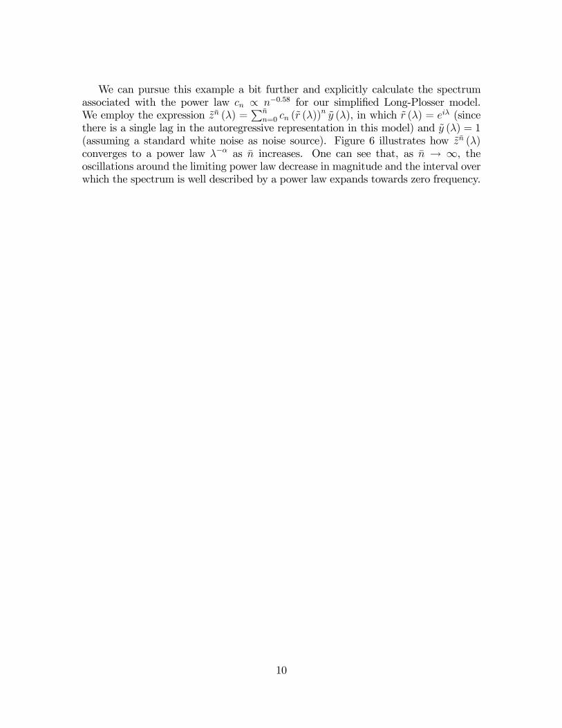
We can pursue this example a bit further and explicitly calculate the spectrum
associated with the power law ∝ −058 for our simplified Long-Plosser model.We employ the expression () =
P
=0 ( ()) (), in which () = (since
there is a single lag in the autoregressive representation in this model) and () = 1
(assuming a standard white noise as noise source). Figure 6 illustrates how ()
converges to a power law − as increases. One can see that, as → ∞, theoscillations around the limiting power law decrease in magnitude and the interval over
which the spectrum is well described by a power law expands towards zero frequency.
10


