1 Suspicion of scientific misconduct by Dr. Jens Förster CONFIDENTIAL – September, 3, 2012 Abstract Here we analyze results from three recent papers (2009, 2011, 2012) by Dr. Jens Förster from the Psychology Department of the University of Amsterdam. These papers report 40 experiments involving a total of 2284 participants (2242 of which were undergraduates). We apply an F test based on descriptive statistics to test for linearity of means across three levels of the experimental design. Results show that in the vast majority of the 42 independent samples so analyzed, means are unusually close to a linear trend. Combined left-tailed probabilities are 0.000000008, 0.0000004, and 0.000000006, for the three papers, respectively. The combined left- tailed p-value of the entire set is p= 1.96 * 10 -21 , which corresponds to finding such consistent results (or more consistent results) in one out of 508 trillion (508,000,000,000,000,000,000). Such a level of linearity is extremely unlikely to have arisen from standard sampling. We also found overly consistent results across independent replications in two of the papers. As a control group, we analyze the linearity of results in 10 papers by other authors in the same area. These papers differ strongly from those by Dr. Förster in terms of linearity of effects and the effect sizes. We also note that none of the 2284 participants showed any missing data, dropped out during data collection, or expressed awareness of the deceit used in the experiment, which is atypical for psychological experiments. Combined these results cast serious doubt on the nature of the results reported by Dr. Förster and warrant an investigation of the source and nature of the data he presented in these and other papers. Papers: Förster, J. (2009). Relations Between Perceptual and Conceptual Scope: How Global Versus Local Processing Fits a Focus on Similarity Versus Dissimilarity. Journal of Experimental Psychology: General, 138, 88-111. Förster, J. (2011). Local and Global Cross-Modal Influences Between Vision and Hearing, Tasting, Smelling, or Touching. Journal of Experimental Psychology: General, 140, 364-389. Förster, J. & Denzler, M. (2012). Sense Creative! The Impact of Global and Local Vision, Hearing, Touching, Tasting and Smelling on Creative and Analytic Thought. Social Psychological and Personality Science, 3, 108-117.
Transcript
1
Suspicion of scientific misconduct by Dr. Jens Förster
CONFIDENTIAL – September, 3, 2012
Abstract
Here we analyze results from three recent papers (2009, 2011, 2012) by Dr. Jens
Förster from the Psychology Department of the University of Amsterdam. These
papers report 40 experiments involving a total of 2284 participants (2242 of which
were undergraduates). We apply an F test based on descriptive statistics to test for
linearity of means across three levels of the experimental design. Results show that in
the vast majority of the 42 independent samples so analyzed, means are unusually
close to a linear trend. Combined left-tailed probabilities are 0.000000008,
0.0000004, and 0.000000006, for the three papers, respectively. The combined left-
tailed p-value of the entire set is p= 1.96 * 10-21, which corresponds to finding such
consistent results (or more consistent results) in one out of 508 trillion
(508,000,000,000,000,000,000). Such a level of linearity is extremely unlikely to
have arisen from standard sampling. We also found overly consistent results across
independent replications in two of the papers. As a control group, we analyze the
linearity of results in 10 papers by other authors in the same area. These papers differ
strongly from those by Dr. Förster in terms of linearity of effects and the effect sizes.
We also note that none of the 2284 participants showed any missing data, dropped
out during data collection, or expressed awareness of the deceit used in the
experiment, which is atypical for psychological experiments. Combined these results
cast serious doubt on the nature of the results reported by Dr. Förster and warrant an
investigation of the source and nature of the data he presented in these and other
papers.
Papers:
Förster, J. (2009). Relations Between Perceptual and Conceptual Scope: How Global
Versus Local Processing Fits a Focus on Similarity Versus Dissimilarity.
Journal of Experimental Psychology: General, 138, 88-111.
Förster, J. (2011). Local and Global Cross-Modal Influences Between Vision and
Hearing, Tasting, Smelling, or Touching. Journal of Experimental
Psychology: General, 140, 364-389.
Förster, J. & Denzler, M. (2012). Sense Creative! The Impact of Global and Local
Vision, Hearing, Touching, Tasting and Smelling on Creative and Analytic
Thought. Social Psychological and Personality Science, 3, 108-117.
2
Statistical approach to test for linearity
The main analyses presented below focus on one-way factorial designs in which
subjects were randomly assigned to three levels (k=3) of an experimental factor and
measured on the same dependent variable. F values from the standard one-way main
effect are computed on the basis of the descriptive statistics in the papers and under
the assumption that the cell sizes are equal1. The between-group mean square (MSB)
can be computed on the basis of the grand mean (xG) and the three cell means (xi)
(B. H. Cohen, 2002, Understanding Statistics):
€
MSB =n (x i∑ − x G )
2
k −1 , (1)
where n represents the (equal) cell size and k the number of groups. F then becomes:
€
F =MSBsi2∑
k
, (2)
where si represents the observed standard deviation in cell i. Under the null
hypothesis of equal population means and variances and (i.i.d.) normality, Equation 2
follows an F distribution with k-2 degrees of freedom in the numerator and k(n – 1)
degrees of freedom in the denominator. Because (MSw = MSB / F), the total sum of
squares can be easily computed: SStot = SSB + SSW = MSW*(k(n-1)) + MSB*(k-1). It
is well known that the one-way ANOVA corresponds to a linear regression with (k-1)
dummy coded predictors. This gives rise to eta-squared:
€
eta2 =SSBSStot
, (3)
or the percentage of variance explained by the categorical independent variable.
1It is quite common in experimental social psychology to assure equal cell sizes, so we consider this an appropriate assumption. Dr. Förster indicated that cell frequencies were identical in the 2012 paper.
3
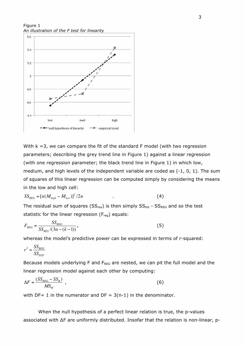
Figure 1 An illustration of the F test for linearity
With k =3, we can compare the fit of the standard F model (with two regression
parameters; describing the grey trend line in Figure 1) against a linear regression
(with one regression parameter; the black trend line in Figure 1) in which low,
medium, and high levels of the independent variable are coded as (-1, 0, 1). The sum
of squares of this linear regression can be computed simply by considering the means
in the low and high cell:
€
SSREG = [n(Mhigh −Mlow )]2 /2n . (4)
The residual sum of squares (SSres) is then simply SStot - SSREG and so the test
statistic for the linear regression (Freg) equals:
€
FREG =SSREG
SSRES /(3n − (k −1)), (5)
whereas the model’s predictive power can be expressed in terms of r-squared:
€
r2 =SSREGSSTOT
Because models underlying F and FREG are nested, we can pit the full model and the
linear regression model against each other by computing:
€
ΔF =(SSREG − SSB )
MSW , (6)
with DF= 1 in the numerator and DF = 3(n-1) in the denominator.
When the null hypothesis of a perfect linear relation is true, the p-values
associated with ∆F are uniformly distributed. Insofar that the relation is non-linear, p-
4
values associated with ∆F will tend towards 0. If empirical results lie too close to the
linear trend line, we expect p-values associated with ∆F to be close to 1.
For each independent sample (or levels within an orthogonal factor; see below),
we computed the ∆F and collected its p-value. The p-values for each sample are
subsequently combined using Fisher’s method:
€
χ p2 = −2 ln(ps)∑ . (7)
The statistics defined in Equation 7 follows a χ2 distribution with twice the number of
samples as degrees of freedom.
Appendix A presents results of a simulation study to verify whether the ∆F test
functions as expected and whether it is robust to violations of normality of the
underlying raw data and rounding of the descriptive statistics that are used as input.
These simulations show no bias that is of concern and so support the validity of the
∆F test.
5
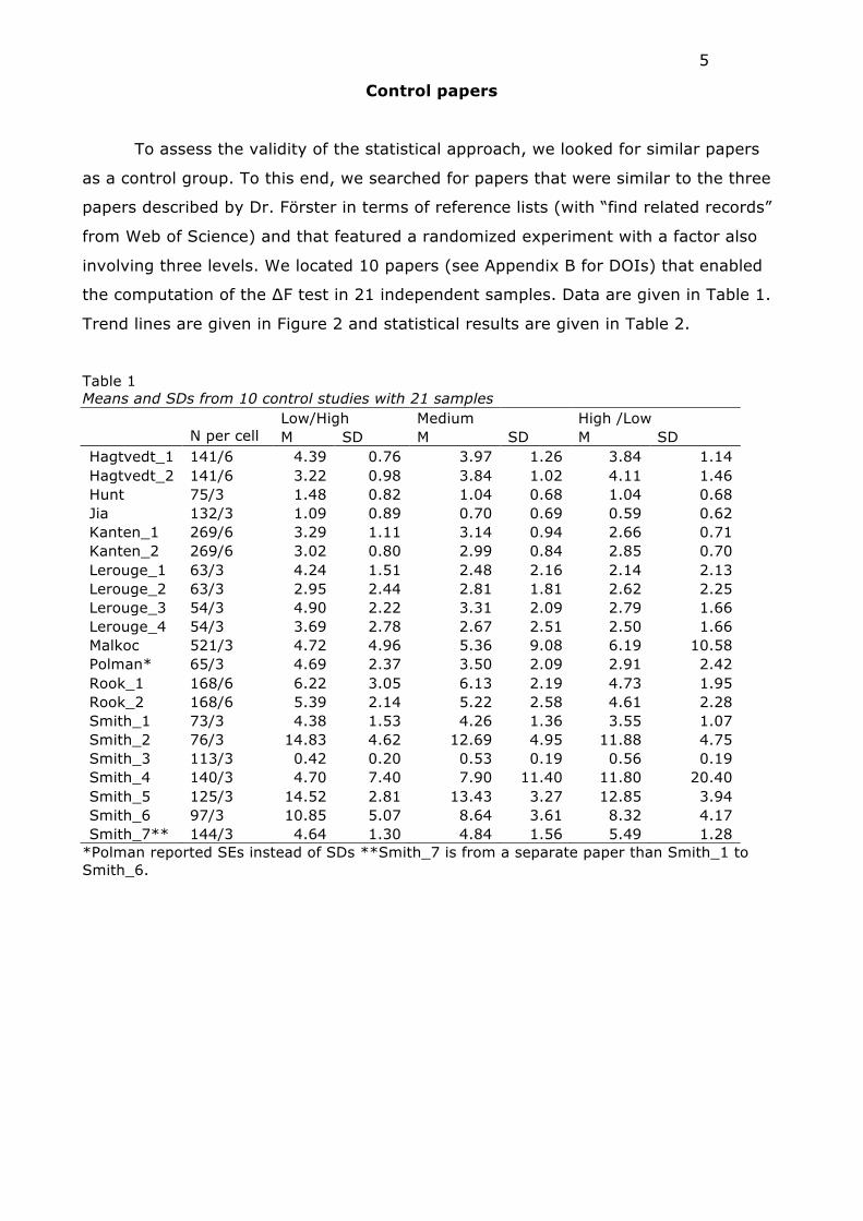
Control papers
To assess the validity of the statistical approach, we looked for similar papers
as a control group. To this end, we searched for papers that were similar to the three
papers described by Dr. Förster in terms of reference lists (with “find related records”
from Web of Science) and that featured a randomized experiment with a factor also
involving three levels. We located 10 papers (see Appendix B for DOIs) that enabled
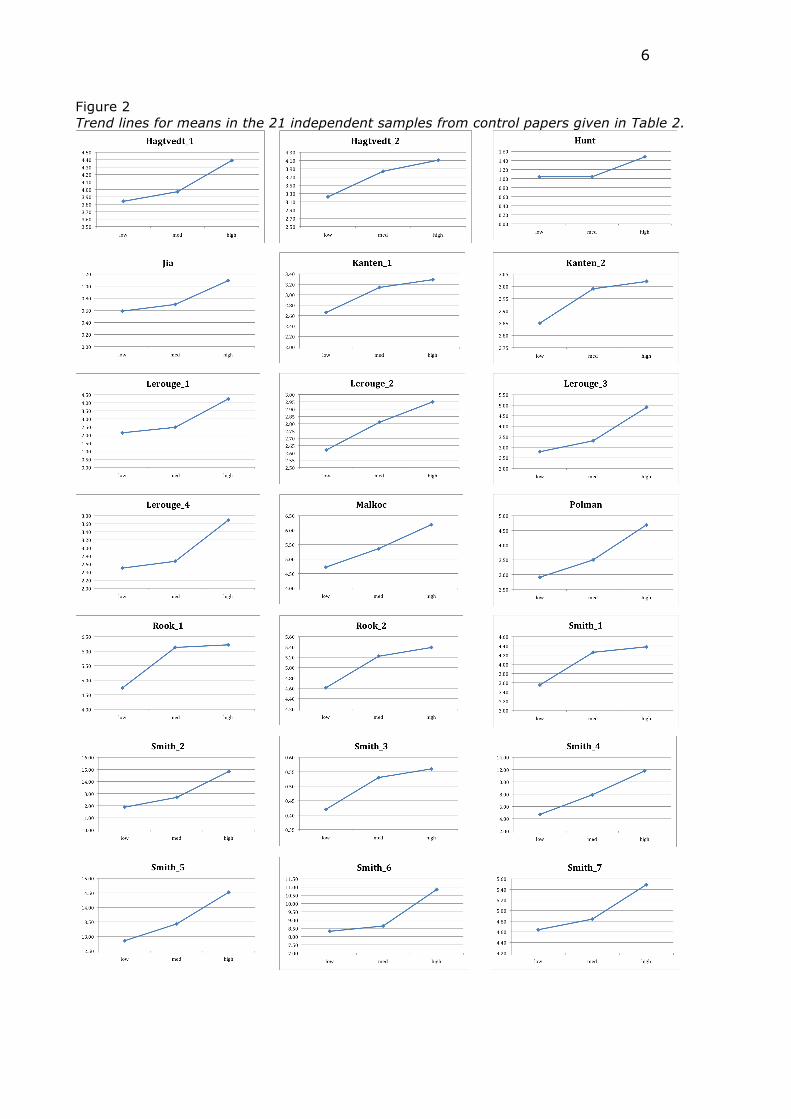
the computation of the ∆F test in 21 independent samples. Data are given in Table 1.
Trend lines are given in Figure 2 and statistical results are given in Table 2.
Freg=5.10. The differences with the recomputed values (on the basis of descriptive
statistics) are minor and can be attributed to rounding. In the case of Jia cell sizes
were unequal.
Eta2 is necessarily larger than or equal to r2. The differences in explained
variance are clear in all control samples except Lerouge_2, where the ∆F test gives a
left-tailed probability of p<.05. One such result is what is expected by chance in 21
samples under the null hypothesis of linearity.
There were five papers with two or more samples that enabled Fisher’s test of a
combined p-value. Results are as follows: Hagtvedt: χ2 (DF = 4) = 2.208, p = .698;
Kanten: χ2 (DF = 4) = 2.890, p = .576; Lerouge: χ2 (DF = 8) = 6.975, p = .559,
Rook: χ2 (DF = 4) = 3.527, p = .474; and Smith: χ2 (DF = 12) = 8.772, p = .722.
Thus, the analyses of results from the ten control papers show results that are to be
expected under the statistical model under the null hypothesis of linearity.
8
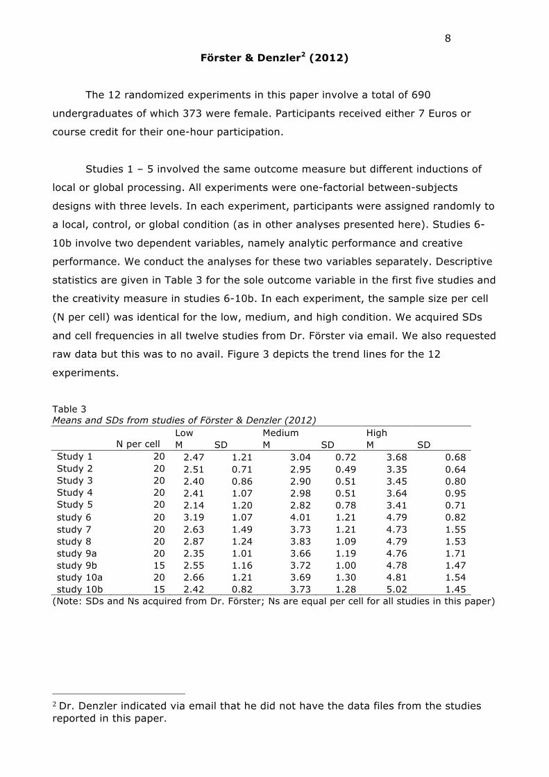
Förster & Denzler2 (2012)
The 12 randomized experiments in this paper involve a total of 690
undergraduates of which 373 were female. Participants received either 7 Euros or
course credit for their one-hour participation.
Studies 1 – 5 involved the same outcome measure but different inductions of
local or global processing. All experiments were one-factorial between-subjects
designs with three levels. In each experiment, participants were assigned randomly to
a local, control, or global condition (as in other analyses presented here). Studies 6-
10b involve two dependent variables, namely analytic performance and creative
performance. We conduct the analyses for these two variables separately. Descriptive
statistics are given in Table 3 for the sole outcome variable in the first five studies and
the creativity measure in studies 6-10b. In each experiment, the sample size per cell
(N per cell) was identical for the low, medium, and high condition. We acquired SDs
and cell frequencies in all twelve studies from Dr. Förster via email. We also requested
raw data but this was to no avail. Figure 3 depicts the trend lines for the 12
experiments.
Table 3 Means and SDs from studies of Förster & Denzler (2012) Low Medium High N per cell M SD M SD M SD Study 1 20 2.47 1.21 3.04 0.72 3.68 0.68 Study 2 20 2.51 0.71 2.95 0.49 3.35 0.64 Study 3 20 2.40 0.86 2.90 0.51 3.45 0.80 Study 4 20 2.41 1.07 2.98 0.51 3.64 0.95 Study 5 20 2.14 1.20 2.82 0.78 3.41 0.71 study 6 20 3.19 1.07 4.01 1.21 4.79 0.82 study 7 20 2.63 1.49 3.73 1.21 4.73 1.55 study 8 20 2.87 1.24 3.83 1.09 4.79 1.53 study 9a 20 2.35 1.01 3.66 1.19 4.76 1.71 study 9b 15 2.55 1.16 3.72 1.00 4.78 1.47 study 10a 20 2.66 1.21 3.69 1.30 4.81 1.54 study 10b 15 2.42 0.82 3.73 1.28 5.02 1.45
(Note: SDs and Ns acquired from Dr. Förster; Ns are equal per cell for all studies in this paper)
2Dr. Denzler indicated via email that he did not have the data files from the studies reported in this paper.
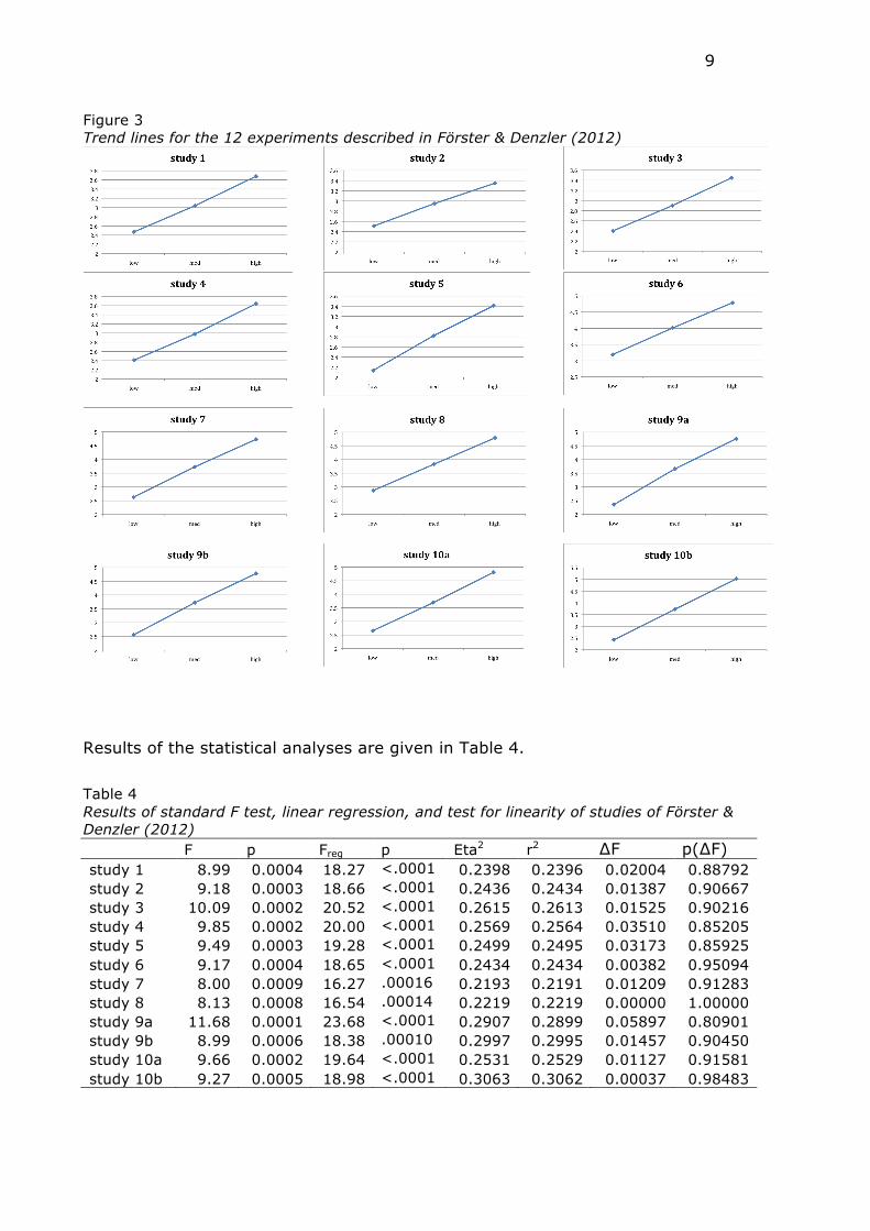
9
Figure 3 Trend lines for the 12 experiments described in Förster & Denzler (2012)
Results of the statistical analyses are given in Table 4.
Table 4 Results of standard F test, linear regression, and test for linearity of studies of Förster & Denzler (2012) F p Freg p Eta2 r2 ∆F p(∆F) study 1 8.99 0.0004 18.27 <.0001 0.2398 0.2396 0.02004 0.88792 study 2 9.18 0.0003 18.66 <.0001 0.2436 0.2434 0.01387 0.90667 study 3 10.09 0.0002 20.52 <.0001 0.2615 0.2613 0.01525 0.90216 study 4 9.85 0.0002 20.00 <.0001 0.2569 0.2564 0.03510 0.85205 study 5 9.49 0.0003 19.28 <.0001 0.2499 0.2495 0.03173 0.85925 study 6 9.17 0.0004 18.65 <.0001 0.2434 0.2434 0.00382 0.95094 study 7 8.00 0.0009 16.27 .00016 0.2193 0.2191 0.01209 0.91283 study 8 8.13 0.0008 16.54 .00014 0.2219 0.2219 0.00000 1.00000 study 9a 11.68 0.0001 23.68 <.0001 0.2907 0.2899 0.05897 0.80901 study 9b 8.99 0.0006 18.38 .00010 0.2997 0.2995 0.01457 0.90450 study 10a 9.66 0.0002 19.64 <.0001 0.2531 0.2529 0.01127 0.91581 study 10b 9.27 0.0005 18.98 <.0001 0.3063 0.3062 0.00037 0.98483
10
The F values reported in the paper were based on raw data whereas our F values were
based on the descriptive statistics rounded to two decimals. The F values in the paper
were 8.93, 9.15, 10.02, 9.85, 9.52, 9.22, 9.01, 8.13, 11.71, 8.99, 9.69, and 9.28,
respectively. All differences are minor except for Study 7 and can be ascribed to
rounding.
As can be seen, the Eta2 and r2 are very close for all studies and all ∆Fs are <.06.
Under the null hypothesis of perfect linearity, we expect the p-values of ∆F tests to be
uniformly distributed between 0 and 1, but in this set of studies all p-values are above
.80. Fisher’s test gives χ2 (DF = 24) = 2.377369693, p = 0.999999994. This means
that given the assumptions of the ∆F test and the model set-up (i.e., there is actual
perfect linearity), such consistent results (or more consistent results) would appear in
only 1 out of 179 million cases.
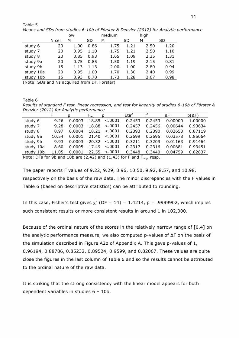
Studies 6-10b involved a second dependent variable called analytic performance. We
conduct a separate analysis for this secondary variable. Results are shown in Figure 4
and Tables 5 and 6.
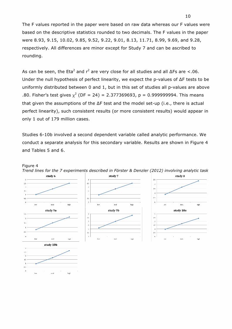
Figure 4 Trend lines for the 7 experiments described in Förster & Denzler (2012) involving analytic task
11
Table 5 Means and SDs from studies 6-10b of Förster & Denzler (2012) for Analytic performance low medium high N cell M SD M SD M SD study 6 20 1.00 0.86 1.75 1.21 2.50 1.20 study 7 20 0.95 1.10 1.75 1.21 2.50 1.10 study 8 20 0.85 0.93 1.65 1.09 2.35 1.31 study 9a 20 0.75 0.85 1.50 1.19 2.15 0.81 study 9b 15 1.13 1.13 2.00 1.00 2.80 0.94 study 10a 20 0.95 1.00 1.70 1.30 2.40 0.99 study 10b 15 0.93 0.70 1.73 1.28 2.67 0.98
(Note: SDs and Ns acquired from Dr. Förster)
Table 6 Results of standard F test, linear regression, and test for linearity of studies 6-10b of Förster & Denzler (2012) for Analytic performance F p Freg p Eta2 r2 ∆F p(∆F) study 6 9.26 0.0003 18.85 <.0001 0.2453 0.2453 0.00000 1.00000 study 7 9.28 0.0003 18.88 <.0001 0.2457 0.2456 0.00644 0.93634 study 8 8.97 0.0004 18.21 <.0001 0.2393 0.2390 0.02653 0.87119 study 9a 10.54 0.0001 21.40 <.0001 0.2699 0.2695 0.03578 0.85064 study 9b 9.93 0.0003 20.32 <.0001 0.3211 0.3209 0.01163 0.91464 study 10a 8.60 0.0005 17.49 <.0001 0.2317 0.2316 0.00681 0.93451 study 10b 11.05 0.0001 22.55 <.0001 0.3448 0.3440 0.04759 0.82837
Note: DFs for 9b and 10b are (2,42) and (1,43) for F and Freg, resp.
The paper reports F values of 9.22, 9.29, 8.96, 10.50, 9.92, 8.57, and 10.98,
respectively on the basis of the raw data. The minor discrepancies with the F values in
Table 6 (based on descriptive statistics) can be attributed to rounding.
In this case, Fisher’s test gives χ2 (DF = 14) = 1.4214, p = .9999902, which implies
such consistent results or more consistent results in around 1 in 102,000.
Because of the ordinal nature of the scores in the relatively narrow range of [0,4] on
the analytic performance measure, we also computed p-values of ∆F on the basis of
the simulation described in Figure A2b of Appendix A. This gave p-values of 1,
0.96194, 0.88786, 0.85232, 0.89524, 0.9599, and 0.82067. These values are quite
close the figures in the last column of Table 6 and so the results cannot be attributed
to the ordinal nature of the raw data.
It is striking that the strong consistency with the linear model appears for both
dependent variables in studies 6 – 10b.
12
Other issues related to Förster & Denzler (2012)
(1) Of the 690 undergraduates, 373 were female. Participants received either 7 Euros
or course credit for their one-hour participation. We note that the University of
Amsterdam has had around 500 psychology freshmen per year in the last five years
and that 72% of these are female (www.uva.nl). The sex distribution in the sample of
Förster & Denzler (2012) (54%) deviates strongly from the sex distribution of
psychology freshmen.
(2) Page 110 of the paper states that “At the end of the entire session, participants
were debriefed; none of them saw any relation between the two phases.” It is
uncommon to find (psychology) undergraduates with no suspicions concerning the
goal of the studies in sample of 690, because these undergraduates are often trained
in psychological research methods. It is also uncommon to have no dropout of
participants or missing data in such a large sample.
(3) “We also explained the distinction between global and local processing to
participants, and asked them to what extent they focused on details versus the whole
during the testing phase on scales anchored at 1 (not at all) and 7 (very much).
Ratings did not differ across conditions in any of the studies, all Fs < 1” and “For
each single experiment, we conducted ONEWAYs to examine effects on moods, or
evaluation of the tasks or inductions. There were no significant effects, all Fs < 1.” It
is unlikely to find F<1 in over 48 F tests even if all null hypotheses were true.
(4) The cognitive test used in experiments 6-10b has only four items, yet the effect
sizes are around d = 1.5, which represent very large effects given the expected low
reliability of the scale. Also, answers are given in an 5-option multiple choice format.
The low means in several conditions (cf. Table 5) suggest that a sizeable portion of
participants performed below chance level, which is peculiar for undergraduates.
(5) Effects are overly consistent across the independent studies despite the fact that
the manipulations are widely different. Also, the two dependent variables in studies 6-
10b show effects that are near mirror images. We ran meta-analyses in Cohen’s d
(with a small-sample size correction due to Hedges & Olkin, 1985) for comparisons of
the low vs. medium, low vs. high, and medium vs. high. In each comparison we ran a
fixed-effects model and computed the Q statistic, which entails a test of homogeneity
13
under the null hypothesis that across each of the five replications the underlying effect
is identical. Results are given in Table 7.
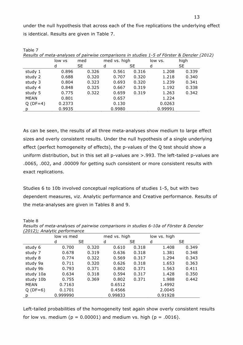
Table 7 Results of meta-analyses of pairwise comparisons in studies 1-5 of Förster & Denzler (2012) low vs med med vs. high low vs. high d SE d SE d SE study 1 0.896 0.326 0.561 0.316 1.208 0.339 study 2 0.688 0.320 0.707 0.320 1.218 0.340 study 3 0.804 0.323 0.693 0.320 1.239 0.341 study 4 0.848 0.325 0.667 0.319 1.192 0.338 study 5 0.775 0.322 0.659 0.319 1.263 0.342 MEAN 0.801 0.657 1.224 Q (DF=4) 0.2373 0.130 0.0263 p 0.9935 0.9980 0.99991
As can be seen, the results of all three meta-analyses show medium to large effect
sizes and overly consistent results. Under the null hypothesis of a single underlying
effect (perfect homogeneity of effects), the p-values of the Q test should show a
uniform distribution, but in this set all p-values are >.993. The left-tailed p-values are
.0065, .002, and .00009 for getting such consistent or more consistent results with
exact replications.
Studies 6 to 10b involved conceptual replications of studies 1-5, but with two
dependent measures, viz. Analytic performance and Creative performance. Results of
the meta-analyses are given in Tables 8 and 9.
Table 8 Results of meta-analyses of pairwise comparisons in studies 6-10a of Förster & Denzler (2012); Analytic performance low vs med med vs. high low vs. high d SE d SE d SE study 6 0.700 0.320 0.610 0.318 1.408 0.349 study 7 0.678 0.319 0.636 0.318 1.381 0.348 study 8 0.774 0.322 0.569 0.317 1.294 0.343 study 9a 0.711 0.320 0.626 0.318 1.653 0.363 study 9b 0.793 0.371 0.802 0.371 1.563 0.411 study 10a 0.634 0.318 0.594 0.317 1.428 0.350 study 10b 0.755 0.369 0.802 0.371 1.988 0.442 MEAN 0.7163 0.6512 1.4992 Q (DF=6) 0.1701 0.4566 2.0045 p 0.999990 0.99833 0.91928
Left-tailed probabilities of the homogeneity test again show overly consistent results
for low vs. medium (p = 0.00001) and medium vs. high (p = .0016).
14
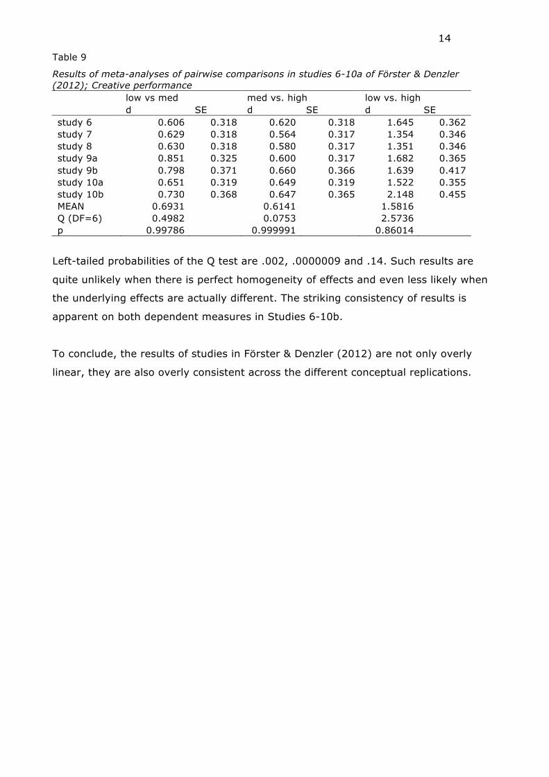
Table 9
Results of meta-analyses of pairwise comparisons in studies 6-10a of Förster & Denzler (2012); Creative performance low vs med med vs. high low vs. high d SE d SE d SE study 6 0.606 0.318 0.620 0.318 1.645 0.362 study 7 0.629 0.318 0.564 0.317 1.354 0.346 study 8 0.630 0.318 0.580 0.317 1.351 0.346 study 9a 0.851 0.325 0.600 0.317 1.682 0.365 study 9b 0.798 0.371 0.660 0.366 1.639 0.417 study 10a 0.651 0.319 0.649 0.319 1.522 0.355 study 10b 0.730 0.368 0.647 0.365 2.148 0.455 MEAN 0.6931 0.6141 1.5816 Q (DF=6) 0.4982 0.0753 2.5736 p 0.99786 0.999991 0.86014
Left-tailed probabilities of the Q test are .002, .0000009 and .14. Such results are
quite unlikely when there is perfect homogeneity of effects and even less likely when
the underlying effects are actually different. The striking consistency of results is
apparent on both dependent measures in Studies 6-10b.
To conclude, the results of studies in Förster & Denzler (2012) are not only overly
linear, they are also overly consistent across the different conceptual replications.
15
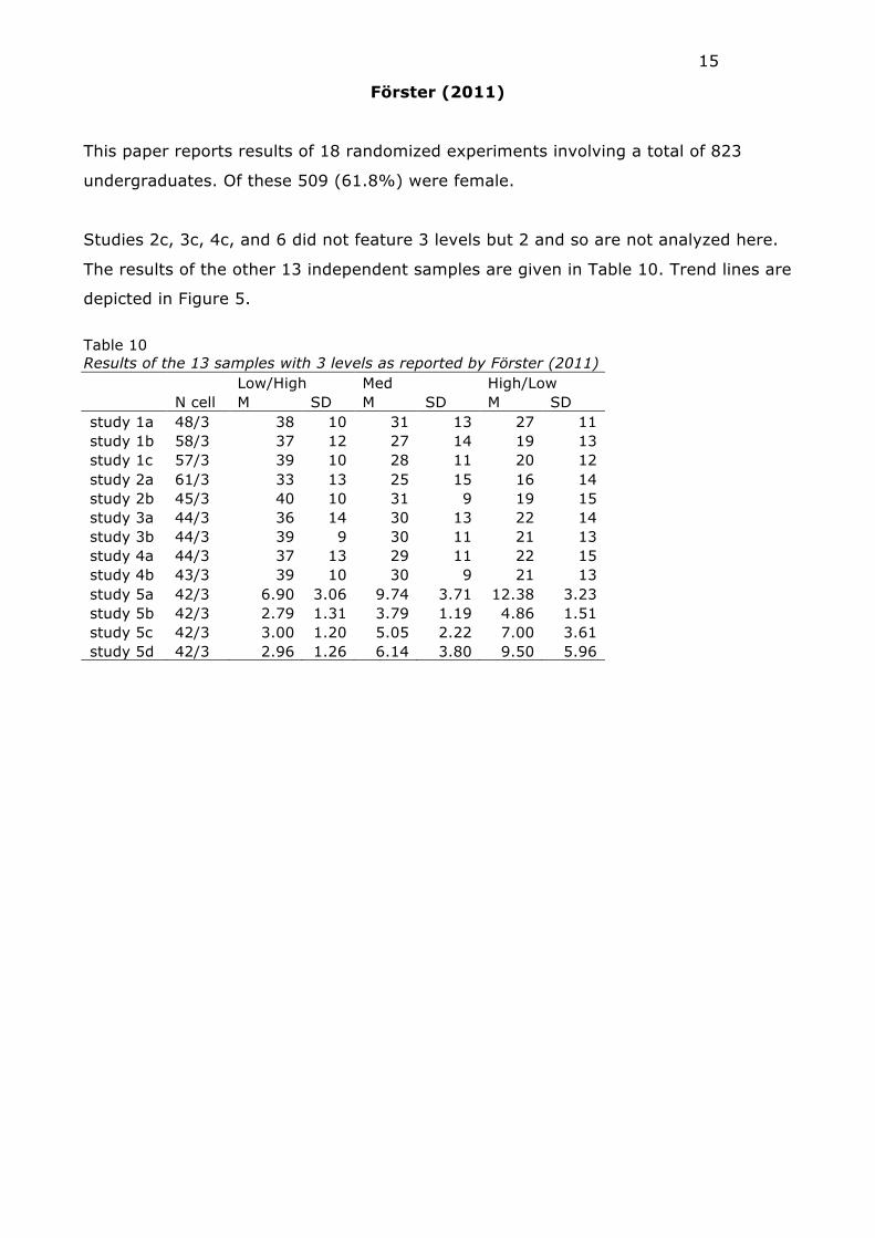
Förster (2011)
This paper reports results of 18 randomized experiments involving a total of 823
undergraduates. Of these 509 (61.8%) were female.
Studies 2c, 3c, 4c, and 6 did not feature 3 levels but 2 and so are not analyzed here.
The results of the other 13 independent samples are given in Table 10. Trend lines are
depicted in Figure 5.
Table 10 Results of the 13 samples with 3 levels as reported by Förster (2011) Low/High Med High/Low N cell M SD M SD M SD study 1a 48/3 38 10 31 13 27 11 study 1b 58/3 37 12 27 14 19 13 study 1c 57/3 39 10 28 11 20 12 study 2a 61/3 33 13 25 15 16 14 study 2b 45/3 40 10 31 9 19 15 study 3a 44/3 36 14 30 13 22 14 study 3b 44/3 39 9 30 11 21 13 study 4a 44/3 37 13 29 11 22 15 study 4b 43/3 39 10 30 9 21 13 study 5a 42/3 6.90 3.06 9.74 3.71 12.38 3.23 study 5b 42/3 2.79 1.31 3.79 1.19 4.86 1.51 study 5c 42/3 3.00 1.20 5.05 2.22 7.00 3.61 study 5d 42/3 2.96 1.26 6.14 3.80 9.50 5.96
16
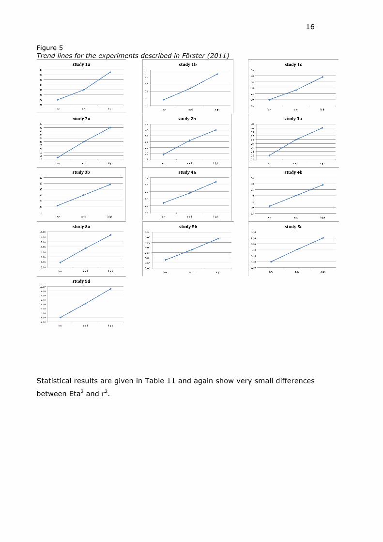
Figure 5 Trend lines for the experiments described in Förster (2011)
Statistical results are given in Table 11 and again show very small differences
between Eta2 and r2.
17
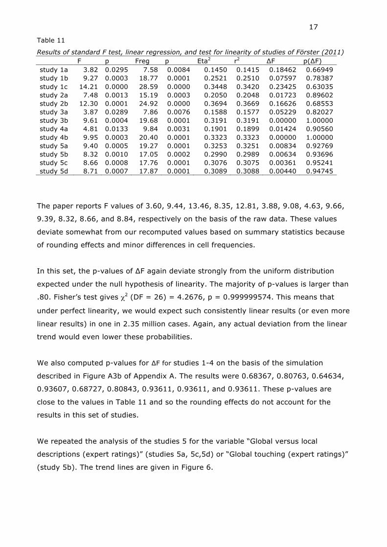
Table 11
Results of standard F test, linear regression, and test for linearity of studies of Förster (2011) F p Freg p Eta2 r2 ∆F p(∆F) study 1a 3.82 0.0295 7.58 0.0084 0.1450 0.1415 0.18462 0.66949 study 1b 9.27 0.0003 18.77 0.0001 0.2521 0.2510 0.07597 0.78387 study 1c 14.21 0.0000 28.59 0.0000 0.3448 0.3420 0.23425 0.63035 study 2a 7.48 0.0013 15.19 0.0003 0.2050 0.2048 0.01723 0.89602 study 2b 12.30 0.0001 24.92 0.0000 0.3694 0.3669 0.16626 0.68553 study 3a 3.87 0.0289 7.86 0.0076 0.1588 0.1577 0.05229 0.82027 study 3b 9.61 0.0004 19.68 0.0001 0.3191 0.3191 0.00000 1.00000 study 4a 4.81 0.0133 9.84 0.0031 0.1901 0.1899 0.01424 0.90560 study 4b 9.95 0.0003 20.40 0.0001 0.3323 0.3323 0.00000 1.00000 study 5a 9.40 0.0005 19.27 0.0001 0.3253 0.3251 0.00834 0.92769 study 5b 8.32 0.0010 17.05 0.0002 0.2990 0.2989 0.00634 0.93696 study 5c 8.66 0.0008 17.76 0.0001 0.3076 0.3075 0.00361 0.95241 study 5d 8.71 0.0007 17.87 0.0001 0.3089 0.3088 0.00440 0.94745
The paper reports F values of 3.60, 9.44, 13.46, 8.35, 12.81, 3.88, 9.08, 4.63, 9.66,
9.39, 8.32, 8.66, and 8.84, respectively on the basis of the raw data. These values
deviate somewhat from our recomputed values based on summary statistics because
of rounding effects and minor differences in cell frequencies.
In this set, the p-values of ∆F again deviate strongly from the uniform distribution
expected under the null hypothesis of linearity. The majority of p-values is larger than
.80. Fisher’s test gives χ2 (DF = 26) = 4.2676, p = 0.999999574. This means that
under perfect linearity, we would expect such consistently linear results (or even more
linear results) in one in 2.35 million cases. Again, any actual deviation from the linear
trend would even lower these probabilities.
We also computed p-values for ∆F for studies 1-4 on the basis of the simulation
described in Figure A3b of Appendix A. The results were 0.68367, 0.80763, 0.64634,
0.93607, 0.68727, 0.80843, 0.93611, 0.93611, and 0.93611. These p-values are
close to the values in Table 11 and so the rounding effects do not account for the
results in this set of studies.
We repeated the analysis of the studies 5 for the variable “Global versus local
(study 5b). The trend lines are given in Figure 6.
18
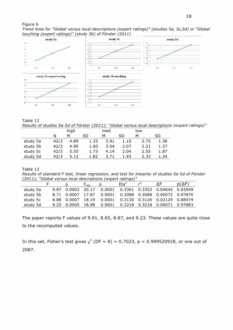
Figure 6 Trend lines for “Global versus local descriptions (expert ratings)” (studies 5a, 5c,5d) or “Global touching (expert ratings)” (study 5b) of Förster (2011)
Table 12 Results of studies 5a-5d of Förster (2011); “Global versus local descriptions (expert ratings)” high med low N M SD M SD M SD study 5a 42/3 4.89 1.33 3.91 1.10 2.75 1.38 study 5b 42/3 4.90 1.60 3.54 2.07 2.21 1.37 study 5c 42/3 5.55 1.73 4.14 2.04 2.55 1.87 study 5d 42/3 5.12 1.82 3.71 1.93 2.33 1.34
Table 13 Results of standard F test, linear regression, and test for linearity of studies 5a-5d of Förster (2011); “Global versus local descriptions (expert ratings)” F p Freg p Eta2 r2 ∆F p(∆F) study 5a 9.87 0.0003 20.17 0.0001 0.3361 0.3353 0.04644 0.83049 study 5b 8.71 0.0007 17.87 0.0001 0.3088 0.3088 0.00072 0.97870 study 5c 8.88 0.0007 18.19 0.0001 0.3130 0.3126 0.02129 0.88474 study 5d 9.25 0.0005 18.98 0.0001 0.3218 0.3218 0.00071 0.97883
The paper reports F values of 9.91, 8.65, 8.87, and 9.23. These values are quite close
to the recomputed values.
In this set, Fisher’s test gives χ2 (DF = 8) = 0.7023, p = 0.999520918, or one out of
2087.
19
Study 5b has a third dependent variable (“Local descriptions (expert ratings)”;
F=8.34) that gives the following results:
Table 14 Results of standard F test, linear regression, and test for linearity of study 5b of Förster (2011); “Local descriptions (expert ratings)” F p Freg p Eta2 r2 ∆F p(∆F) study 5b 8.29 0.0007 16.99 0.0001 0.2983 0.2982 0.00059 0.98072
So the near-perfect linearity (p>.97) in study 5b reappears on all three dependent
variables.
20
Other issues related to Förster (2011)
(1) Of the 823 undergraduates, 509 (61.8%) were female. The sex distribution in the
sample deviates from the sex distribution of psychology freshmen at the University of
Amsterdam.
(2) All 823 participating undergraduates were probed for suspicion concerning the
relation between the tasks in the experiment. None of them saw any relation between
the tasks. This is highly unlikely in such a large sample containing undergraduates
who are typically trained in psychological research methods and who are often quite
experienced as research participants. The lack of missing data and dropout is also not
characteristic of psychological experiments of this type in such a large sample.
(3) The paper reports a disproportionally large number of F tests with values < 1,
which is not to be expected even if all null hypotheses were true.
(4) Effects are overly consistent across the independent studies despite the fact that
the manipulations are widely different. We ran meta-analyses in Cohen’s d (with a
small-sample size correction due to Hedges & Olkin, 1985) for comparisons of the low
vs. medium, low vs. high, and medium vs. high conditions. In each comparison we
ran a fixed-effects model and computed the Q statistic, which entails a test of
homogeneity under the null hypothesis that across each of the replications the
underlying effect is identical. Results are given in Table 15 for studies 5a-5b. Table 16
gives the results of studies with “explicit manipulations” (as categorized by Förster,
2011 on page 379). Table 17 gives the results of studies with “implicit manipulations”
(as categorized by Förster, 2011 on page 379).
In each set, we find overly consistent results.
Table 15 Results of meta-analyses of pairwise comparisons in studies 5a-5d of Förster (2011) low vs. med med vs high low vs high d SE d SE d SE Study 5a 0.811 0.384 0.737 0.381 1.691 0.435 Study 5b 0.776 0.382 0.764 0.382 1.422 0.416 Study 5c 1.115 0.398 0.632 0.377 1.444 0.417 Study 5d 1.091 0.396 0.653 0.378 1.474 0.419 MEAN 0.9424 0.6958 1.5039 Q (DF=3) 0.6365 0.0856 0.2504 p 0.8880 0.9935 0.9691
21
Table 16 Results of meta-analyses of pairwise comparisons in studies with explicit manipulations in Förster (2011) low vs med med vs high low vs high d SE d SE d SE Study 1a 0.588 0.353 0.324 0.347 1.020 0.369 Study 2a 0.559 0.314 0.608 0.315 1.234 0.338 Study 3a 0.432 0.364 0.576 0.367 0.972 0.382 Study 4a 0.646 0.369 0.517 0.366 1.039 0.385 MEAN 0.5563 0.5096 1.0765 Q (DF=3) 0.1844 0.4173 0.3243 p 0.9801 0.9366 0.9554
Table 17 Results of meta-analyses of pairwise comparisons in studies with implicit manipulations in Förster (2011) low vs med med vs high low vs high d SE d SE d SE Study 1b 0.751 0.327 0.580 0.322 1.409 0.355 Study 1c 1.024 0.340 0.680 0.327 1.684 0.374 Study 2b 0.920 0.376 0.944 0.377 1.603 0.414 Study 2c* 0.784 0.336 Study 3b 0.871 0.378 0.727 0.372 1.565 0.416 Study 4b 0.919 0.384 0.782 0.378 1.506 0.414 Study 4c* 0.894 0.383 MEAN 0.8938 0.7285 1.3162 Q (DF=4/6) 0.3517 0.5813 5.8061 p 0.9862 0.9651 0.4453
Note: *Studies 2c and 4c do not feature an intermediate control group.
So in Tables 15, 16, and 17, we found p-values that lie close to one, indicating
that the results in (conceptual) replications reported by Förster (2011) are overly
consistent. The left-tailed p-values are based on perfect homogeneity of effects, so
they would be even smaller when in actuality the underlying effects are
heterogeneous.
What is remarkable about the result in Table 17 is that the effects are similar
when the experiment involved a control group (cf. comparisons of low vs med and
med vs. high), but not when the control group was omitted (studies 2c and 4c).
To conclude, the results presented in Förster (2011) show overly linear trends and
show overly strong consistencies across conceptual replications.
22
Förster (2009)
This paper reports a total of 12 experiments, involving 736 undergraduates and 42
business managers. The designs of the experiments are given in Table 18.
Table 18 Designs of experiments by Förster (2009) Study 1st factor 2nd factor 1 3 between 2 within 2 3 between 2 between 3a 3 between 2 between 3b 3 between 2 between 4 3 between 2 within 5 3 between 2 within 6 3 between - 7a 3 between 2 between 7b 3 between 2 within 8a 2 between 2 between 8b 3 between 2 between 9 3 between 2 between
Analyses involved all but study 8a, which had only 2 factors. Given that the second
factor was between-subject (implying independence of data points), studies 2, 3a, 3b,
7a, 8b, and 9 present two independent samples, giving a total of 17 samples.
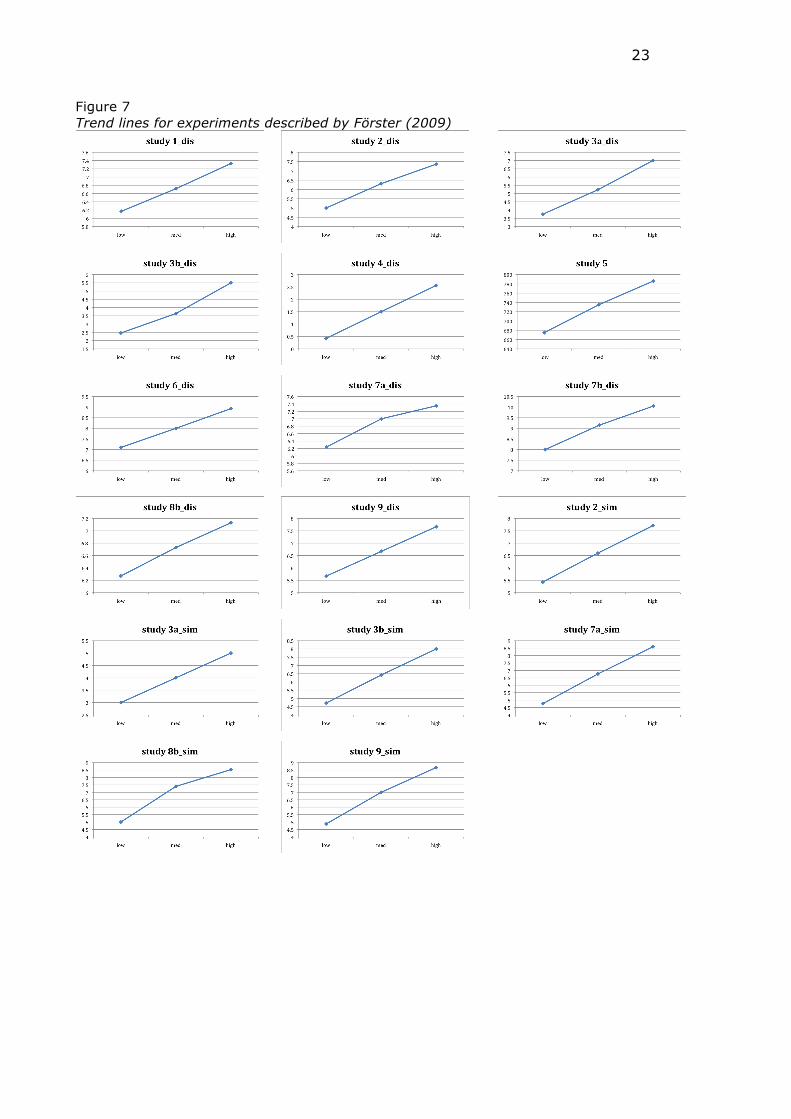
Descriptive statistics are given in Table 19 and trend lines in Figure 7.
Table 19 Results of the 17 independent samples with 3 levels as reported by Förster (2009) High/low med Low/high N cell M SD M SD M SD study 1_dis 54/3 7.33 3.22 6.72 2.74 6.17 3.54 study 2_dis 88/6 7.36 1.86 6.31 2.77 5.00 2.08 study 3a_dis 75/6 7.00 0.95 5.23 1.83 3.75 2.18 study 3b_dis 71/6 5.50 1.62 3.64 1.43 2.46 1.56 study 4_dis 55/3 2.56 2.36 1.50 1.15 0.42 0.90 study 5_loc 50/3 675 63 735 63 786 86 study 6_dis 42/3 7.10 1.14 8.00 1.62 8.93 0.83 study 7a_dis 101/6 7.35 3.14 7.00 2.80 6.24 3.56 study 7b_dis 60/3 10.05 3.25 9.15 3.01 8.00 1.95 study 8b_dis 45/6 7.13 2.20 6.73 1.87 6.27 2.02 study 9_dis 90/6 7.67 3.11 6.67 2.47 5.67 2.97 study 2_sim 88/6 5.43 1.83 6.60 3.16 7.71 3.93 study 3a_sim 75/6 3.00 1.29 4.00 1.54 5.00 0.71 study 3b_sim 71/6 4.72 1.42 6.42 1.88 8.00 2.49 study 7a_sim 101/6 4.76 2.39 6.76 2.46 8.59 2.09 study 8b_sim 45/6 5.00 2.00 7.40 2.32 8.53 1.73 study 9_sim 90/6 4.87 2.17 7.00 2.23 8.67 2.06
Note: dis: dissimilarity; sim: similarity; loc: local
23
Figure 7 Trend lines for experiments described by Förster (2009)
24
Table 20 Results of standard F test, linear regression, and test for linearity of studies in Förster (2009) F p Freg p Eta2 r2 ∆F p(∆F) study 1_dis 0.60 0.5538 1.22 0.0025 0.0229 0.0229 0.00107 0.97409 study 2_dis 3.98 0.0263 8.11 0.0284 0.1626 0.1619 0.03207 0.85876 study 3a_dis 11.03 0.0002 22.60 0.0920 0.3900 0.3889 0.05838 0.81053 study 3b_dis 11.74 0.0002 23.53 0.1334 0.4194 0.4126 0.38518 0.53924 study 4_dis 8.18 0.0008 16.67 0.1150 0.2392 0.2392 0.00048 0.98268 study 5_loc 10.07 0.0002 20.50 0.0000 0.2999 0.2992 0.04402 0.83472 study 6_dis 7.62 0.0016 15.64 0.2222 0.2811 0.2810 0.00137 0.97071 study 7a_dis 0.54 0.5889 1.04 0.0026 0.0220 0.0211 0.04658 0.83006 study 7b_dis 2.70 0.0755 5.47 0.0070 0.0867 0.0862 0.02668 0.87083 study 8b_dis 0.34 0.7191 0.70 0.0554 0.0333 0.0332 0.00109 0.97404 study 9_dis 1.83 0.1730 3.75 0.0065 0.0801 0.0801 0.00000 1.00000 study 2_sim 1.99 0.1500 4.07 0.0035 0.0884 0.0884 0.00092 0.97598 study 3a_sim 8.26 0.0012 17.00 0.2268 0.3238 0.3238 0.00000 1.00000 study 3b_sim 8.13 0.0014 16.75 0.0562 0.3334 0.3333 0.00725 0.93267 study 7a_sim 11.49 0.0001 23.44 0.0247 0.3260 0.3258 0.01508 0.90279 study 8b_sim 5.91 0.0101 11.62 0.0558 0.3773 0.3617 0.48875 0.49296 study 9_sim 11.72 0.0001 23.82 0.0368 0.3582 0.3565 0.11396 0.73736
Differences between Eta2 and r2 are again very small except in samples study 3b_dis
and study_8b_sim. In the preponderance of samples the p-values associated with the
∆F test are >.90.
Fisher’s test gives χ2 (DF = 34) = 5.5864, p = 0.999999992, or 1 out of 128 million.
Any actual deviation from linearity would lower the left-tailed probabilities and hence
lower the overall probability.
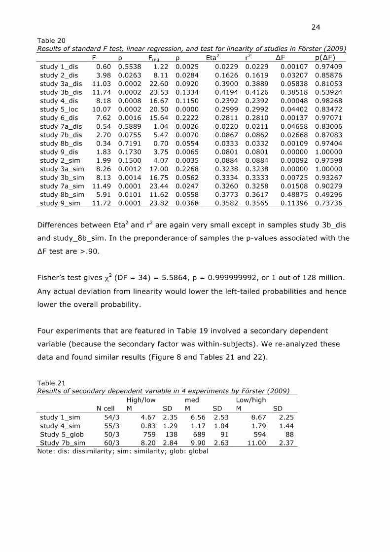
Four experiments that are featured in Table 19 involved a secondary dependent
variable (because the secondary factor was within-subjects). We re-analyzed these
data and found similar results (Figure 8 and Tables 21 and 22).
Table 21 Results of secondary dependent variable in 4 experiments by Förster (2009) High/low med Low/high N cell M SD M SD M SD study 1_sim 54/3 4.67 2.35 6.56 2.53 8.67 2.25 study 4_sim 55/3 0.83 1.29 1.17 1.04 1.79 1.44 Study 5_glob 50/3 759 138 689 91 594 88 Study 7b_sim 60/3 8.20 2.84 9.90 2.63 11.00 2.37
Note: dis: dissimilarity; sim: similarity; glob: global
25
Figure 8 Trend lines of secondary dependent variable in 4 experiments by Förster (2009)
Table 22 Results of standard F test, linear regression, and test for linearity of studies with a secondary dependent variable in Förster (2009) F p Freg p Eta2 r2 ∆F p(∆F) study 1_sim 12.73 0.0000 25.92 0.0210 0.3330 0.3326 0.02564 0.87340 study 4_sim 2.70 0.0763 5.34 0.2105 0.0942 0.0916 0.14912 0.70095 study 5_glob 9.78 0.0003 19.76 0.0000 0.2938 0.2916 0.14852 0.70170 study 7b_sim 5.80 0.0051 11.58 0.0112 0.1690 0.1665 0.17476 0.67748
Again, the similarity of overly linear results across two dependent variables is striking.
26
Other issues related to Förster (2009)
(1) All participants were probed for suspicion concerning the goal of the studies. None
of the 736 undergraduates and 42 business managers raised the possibility that the
different study phases were related. This is quite unexpected in such a large sample
containing undergraduates who are often trained in psychological research methods
and are experienced as participants.
(2) The paper does not report any dropout or missing data among any of the 778
participants. This is atypical of psychological experiments.
27
Discussion
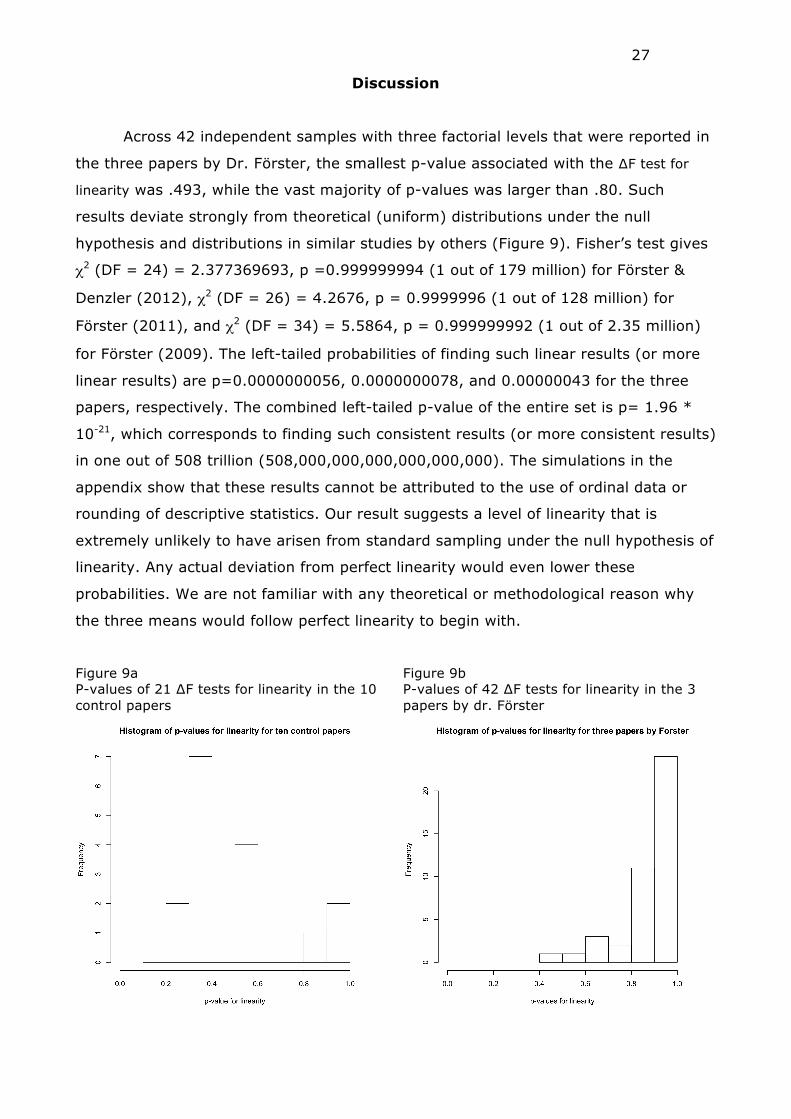
Across 42 independent samples with three factorial levels that were reported in
the three papers by Dr. Förster, the smallest p-value associated with the ∆F test for
linearity was .493, while the vast majority of p-values was larger than .80. Such
results deviate strongly from theoretical (uniform) distributions under the null
hypothesis and distributions in similar studies by others (Figure 9). Fisher’s test gives
χ2 (DF = 24) = 2.377369693, p =0.999999994 (1 out of 179 million) for Förster &
Denzler (2012), χ2 (DF = 26) = 4.2676, p = 0.9999996 (1 out of 128 million) for
Förster (2011), and χ2 (DF = 34) = 5.5864, p = 0.999999992 (1 out of 2.35 million)
for Förster (2009). The left-tailed probabilities of finding such linear results (or more
linear results) are p=0.0000000056, 0.0000000078, and 0.00000043 for the three
papers, respectively. The combined left-tailed p-value of the entire set is p= 1.96 *
10-21, which corresponds to finding such consistent results (or more consistent results)
in one out of 508 trillion (508,000,000,000,000,000,000). The simulations in the
appendix show that these results cannot be attributed to the use of ordinal data or
rounding of descriptive statistics. Our result suggests a level of linearity that is
extremely unlikely to have arisen from standard sampling under the null hypothesis of
linearity. Any actual deviation from perfect linearity would even lower these
probabilities. We are not familiar with any theoretical or methodological reason why
the three means would follow perfect linearity to begin with.
Figure 9a P-values of 21 ∆F tests for linearity in the 10 control papers
Figure 9b P-values of 42 ∆F tests for linearity in the 3 papers by dr. Förster
28
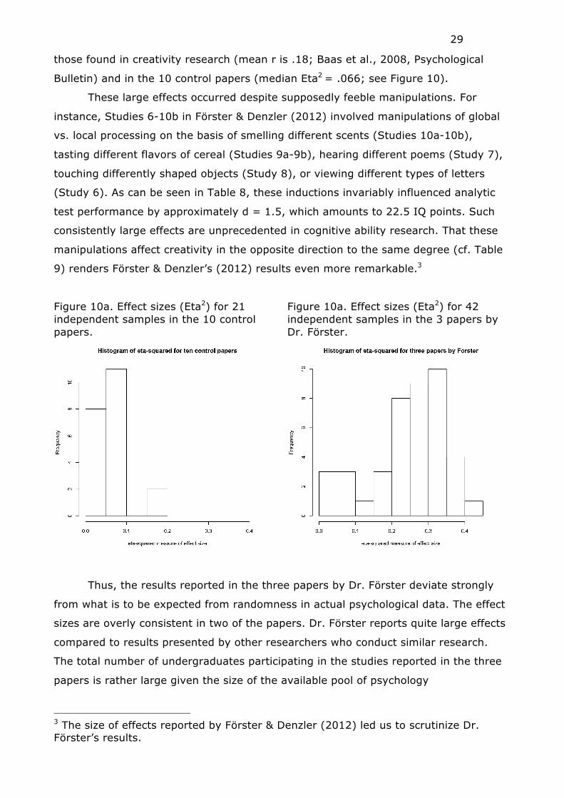
Given the exceptionally large number of studies and undergraduates who
participated in these studies (2242; while the UvA has only around 500 psychology
freshmen per cohort), publication bias (i.e., the notion that Dr. Förster published only
the most linear findings from a larger set of studies) is an unlikely explanation for the
current results. We also note that the cost of data collection (materials, personnel
cost, and financial rewards for participants) must have been substantial. Dr. Förster
employs identical or highly similar outcome measures across different studies. We
consider it unlikely that he selected in each study the most linear outcome measure
from a subset of outcome measures. In fact, seven of the studies from Förster &
Denzler (2012), four studies from Förster (2011), and four studies from Förster
(2009) entailed two dependent variables, both of which showed the exact same overly
strong level of linearity. In one sample, all three outcome measures showed the same
unexpectedly high level of linearity.
None of the 2242 participating undergraduates raised any suspicions
concerning the goal of the studies or the deceit used in the experiments. Given their
education in (psychological) research methods and their expected seasonality as
research participants, we consider this an extremely unlikely outcome. Also, there is
no mention of dropout or missing data in any of the studies (except for a few
participants who were allergic to particular foods and hence did not participate), which
is not characteristic for psychological experiments of durations of 1 to 2 hours.
Although the origin of the undergraduates is not explicated, it is likely that they were
(predominantly) from the University of Amsterdam, at least for the 2011 and 2012
papers. The sex distribution in the 2011 and 2012 papers deviates from the sex
distribution of psychology freshmen at the University of Amsterdam in the years since
Dr. Förster arrived there. All participants were debriefed after each experiment, so it
is implausible that undergraduates returned for later experiments by Dr. Förster
without any of them expressing awareness of the research hypothesis of (or the
deceit used in) the later experiment. So the number of undergraduates participating
in the 40 experiments cannot be attributed to the reuse of undergraduates from the
same pool of participants. This raises further questions about the origin of the data.
Our meta-analyses showed overly consistent findings across widely different
replications in Förster & Denzler (2012) and Förster (2011). So not only are these
results too linear, they are also overly similar across conceptual replications.
Moreover, effect sizes reported by Dr. Förster (median Eta2 for the 2009, 2011, and
2012 papers were .281, .308, and .252, respectively) are quite large in comparison to
29
those found in creativity research (mean r is .18; Baas et al., 2008, Psychological
Bulletin) and in the 10 control papers (median Eta2 = .066; see Figure 10).
These large effects occurred despite supposedly feeble manipulations. For
instance, Studies 6-10b in Förster & Denzler (2012) involved manipulations of global
vs. local processing on the basis of smelling different scents (Studies 10a-10b),
tasting different flavors of cereal (Studies 9a-9b), hearing different poems (Study 7),
touching differently shaped objects (Study 8), or viewing different types of letters
(Study 6). As can be seen in Table 8, these inductions invariably influenced analytic
test performance by approximately d = 1.5, which amounts to 22.5 IQ points. Such
consistently large effects are unprecedented in cognitive ability research. That these
manipulations affect creativity in the opposite direction to the same degree (cf. Table
9) renders Förster & Denzler’s (2012) results even more remarkable.3
Figure 10a. Effect sizes (Eta2) for 21 independent samples in the 10 control papers.
Figure 10a. Effect sizes (Eta2) for 42 independent samples in the 3 papers by Dr. Förster.
Thus, the results reported in the three papers by Dr. Förster deviate strongly
from what is to be expected from randomness in actual psychological data. The effect
sizes are overly consistent in two of the papers. Dr. Förster reports quite large effects
compared to results presented by other researchers who conduct similar research.
The total number of undergraduates participating in the studies reported in the three
papers is rather large given the size of the available pool of psychology
3 The size of effects reported by Förster & Denzler (2012) led us to scrutinize Dr. Förster’s results.
30
undergraduates at the University of Amsterdam (around 500 per year) and the sex
distribution in Dr. Förster’s samples deviates from the sex distribution among
psychology students at the University of Amsterdam. It is unusual that none of the
participating students raised any suspicions about the experimental design and
hypothesis. The lack of dropout or missing data is atypical for psychological
experiments of this type.
The extraordinary nature of results presented by Dr. Förster in these three
papers raise the possibility of improper conduct and warrant an investigation of the
source and nature of the data he presented in these and other papers.
31
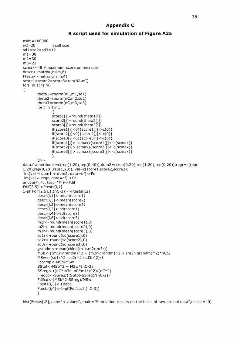
Appendix A
Simulations to assess robustness against rounding and non-normality
We ran several simulations to determine the robustness of the approach to
deviations of normality of the underlying raw data and rounding of the descriptive
statistics. In the first simulation, we simulated random normal data without rounding
and the following distributions: Low ~ N(90,15); Medium ~ N(100,15); High ~
N(110,15), with cell sizes n = 20. All simulations are based on 100,000 runs. The
distribution of the p-values of ∆F are given in Figure A1a and show the expected
uniform distribution both when the ∆F was based on the raw data (Figure A1a; no
rounding of descriptive statistics) and when ∆F was based on descriptive statistics
rounded to two decimals (Figure A1b).
Figure A1a. Distribution of p-values
of ∆F under the null hypothesis,
normal raw data and no rounding of
descriptive statistics.
Figure A1b. Distribution of p-values
of ∆F under the null hypothesis,
normal data and rounding of descriptive
statistics (2 decimals).
Next, we simulated random normal data (again with n = 20 in each cell) with
Low ~ N(1,1); Medium ~ N(1.75,1); High ~ N(2.5,1) and subsequently rounded the
raw data to integers and bounded the scores to the interval [0,4]. This aligns with
results from the analytic performance measure in studies 6-10b of Förster & Denzler
(2012) and represents the most severe rounding of raw data in all studies described
below. Figure 4 gives the distribution of the p-values of ∆F under this set-up on the
32
basis of raw data (Figure A2a) and on the basis of descriptive statistics that were
rounded to two decimals (Figure A2b).
Figure A2a. Distribution of p-values
of ∆F under the null hypothesis,
ordinal raw data and no rounding of
descriptive statistics.
Figure A2b. Distribution of p-values
of ∆F under the null hypothesis,
ordinal data and rounding of descriptive
statistics (2 decimals).
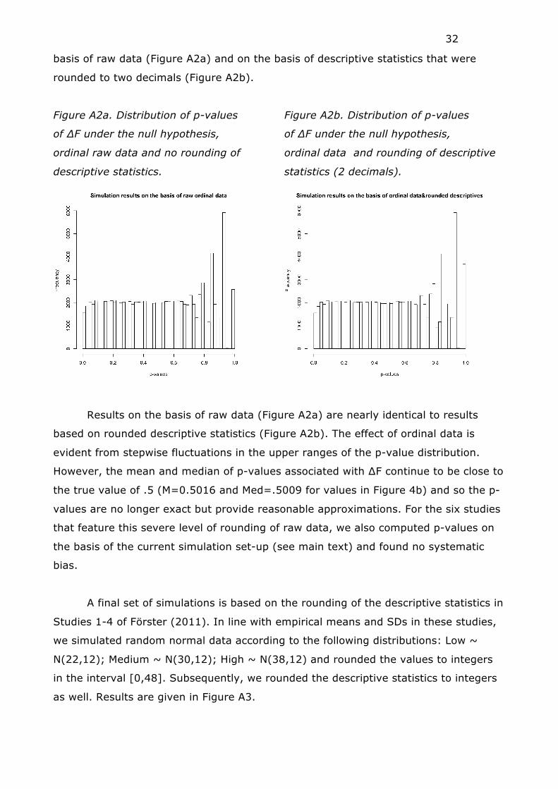
Results on the basis of raw data (Figure A2a) are nearly identical to results
based on rounded descriptive statistics (Figure A2b). The effect of ordinal data is
evident from stepwise fluctuations in the upper ranges of the p-value distribution.
However, the mean and median of p-values associated with ∆F continue to be close to
the true value of .5 (M=0.5016 and Med=.5009 for values in Figure 4b) and so the p-
values are no longer exact but provide reasonable approximations. For the six studies
that feature this severe level of rounding of raw data, we also computed p-values on
the basis of the current simulation set-up (see main text) and found no systematic
bias.
A final set of simulations is based on the rounding of the descriptive statistics in
Studies 1-4 of Förster (2011). In line with empirical means and SDs in these studies,
we simulated random normal data according to the following distributions: Low ~
N(22,12); Medium ~ N(30,12); High ~ N(38,12) and rounded the values to integers
in the interval [0,48]. Subsequently, we rounded the descriptive statistics to integers
as well. Results are given in Figure A3.
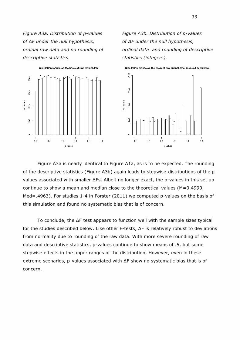
33
Figure A3a. Distribution of p-values
of ∆F under the null hypothesis,
ordinal raw data and no rounding of
descriptive statistics.
Figure A3b. Distribution of p-values
of ∆F under the null hypothesis,
ordinal data and rounding of descriptive
statistics (integers).
Figure A3a is nearly identical to Figure A1a, as is to be expected. The rounding
of the descriptive statistics (Figure A3b) again leads to stepwise-distributions of the p-
values associated with smaller ∆Fs. Albeit no longer exact, the p-values in this set up
continue to show a mean and median close to the theoretical values (M=0.4990,
Med=.4963). For studies 1-4 in Förster (2011) we computed p-values on the basis of
this simulation and found no systematic bias that is of concern.
To conclude, the ∆F test appears to function well with the sample sizes typical
for the studies described below. Like other F-tests, ∆F is relatively robust to deviations
from normality due to rounding of the raw data. With more severe rounding of raw
data and descriptive statistics, p-values continue to show means of .5, but some
stepwise effects in the upper ranges of the distribution. However, even in these
extreme scenarios, p-values associated with ∆F show no systematic bias that is of