J. Ortega-Casanova, N. Campos and R. Fernandez-Feria

Swirling jet models based on experimental measurements at the exit of swirl vane nozzles

J. Ortega-Casanova jortega@uma.esE.T.S. De Ingeniería Industrial. Universidad de Málaga. Málaga, 29071, SpainN. Campos nicalon@hotmail.comE.T.S. De Ingeniería Industrial. Universidad de Málaga. Málaga, 29071, SpainR. Fernandez-Feria ramon.fernandez@uma.esE.T.S. De Ingeniería Industrial. Universidad de Málaga. Málaga, 29071, Spain

AbstractSwirling jets generated by swirl vane nozzles are of interest in many industrial applications. The accurate modeling of their velocity fields is essential for the design of these devices and their associated vortex flow. In this paper we present a series of models of both the axial and the azimuthal velocity components based on accurate measurements by LDA of the velocity fields at the exit of several swirl vane nozzle configurations. These models are based on Batchelor’s vortex solution [2], whose different non-dimensional parameters are discussed as functions of the Reynolds number and the swirl vane configuration.

Keywords: swirling jet, swirl vane nozzle, LDA, industrial applications.

1. INTRODUCTIONSwirling flows are of interest in many industrial processes such as those involving combustion, separation, propulsion, cooling, cleaning, excavation, etc. The swirl is commonly generated by some kind of guided-blades [8], or by rotating some solid parts of the device [5], or by entering the fluid radially to the device [4], among other configurations, depending on the particular industrial application. To design these industrial devices, and to simulate their corresponding internal or external flow, it is essential to have some accurate model for the swirling flow entering or exiting them. Also, these models are of theoretical interest to predict the flow patterns associated to hydrodynamic instabilities of swirling jets.In this work we consider the swirling flow generated by a nozzle where the tangential velocity is imparted to the flow by the use of swirl vanes with adjustable angles. This type of device is common to generate swirling jets in several industrial applications, but in this work was motivated by seabed excavation devices that use a swirl component to enhance their excavation performance [13,11].The objective of this work is to characterize the velocity profiles of the jets generated by different combinations of swirl vanes in wide a range of Reynolds numbers. To that end, we measure both the azimuthal and axial velocity profiles at the exit of the nozzle using Laser Doppler Anemometry (LDA) for the different configurations and Reynolds numbers. Then, we fit these velocity profiles to different swirling jet models. It is shown that the best fit in most of the cases considered is obtained by using a Batchelor's vortex model [2], but with its tail modified with a tanh-like mixing layer that adjust the flow to the external fluid at rest.

2. EXPERIMENTSWe have performed a series of experiments to characterize the velocity structure of swirling jets discharging from a swirl generator nozzle into a quiescent tank of water where the nozzle is submerged. We use a tank with a square base of area 1 m2 and 0.5 m deep. The surfaces of the tank are made of plexiglass to allow for the velocity measurements with LDA. The size of the tank is large enough for the nozzle exit to be sufficiently far from the bottom and lateral walls of the tank, and from the upper free surface open to the atmosphere, thus minimizing their effects on the swirling jet at the nozzle exit.Water is recirculated with a low pressure magnetically-coupled pump. It goes out of the tank through two orifices at the upper part of the lateral surfaces and is decanted into a small auxiliary deposit. From this deposit, after passing through a stop valve, it is impelled by the recirculation pump to the swirl generator nozzle inside the tank. A stop valve is also incorporated downstream of the pump, in addition to an

International Congress on Vortex Flow and Vortex Methods 1

J. Ortega-Casanova, N. Campos and R. Fernandez-Feria

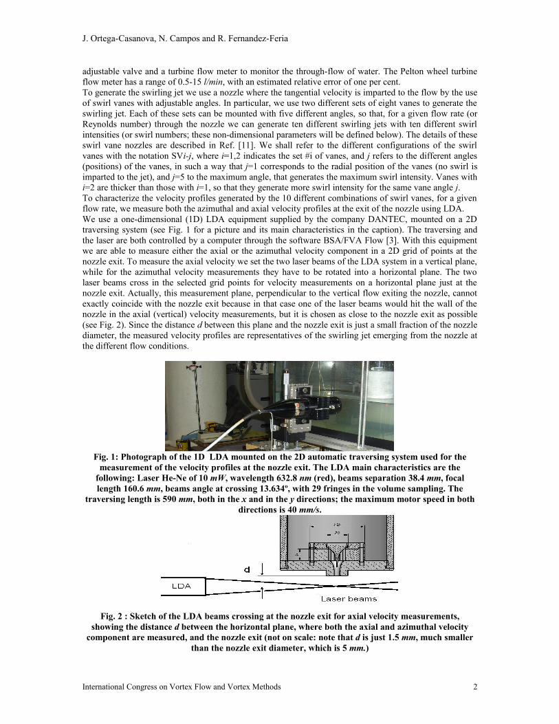
adjustable valve and a turbine flow meter to monitor the through-flow of water. The Pelton wheel turbine flow meter has a range of 0.5-15 l/min, with an estimated relative error of one per cent.To generate the swirling jet we use a nozzle where the tangential velocity is imparted to the flow by the use of swirl vanes with adjustable angles. In particular, we use two different sets of eight vanes to generate the swirling jet. Each of these sets can be mounted with five different angles, so that, for a given flow rate (or Reynolds number) through the nozzle we can generate ten different swirling jets with ten different swirl intensities (or swirl numbers; these non-dimensional parameters will be defined below). The details of these swirl vane nozzles are described in Ref. [11]. We shall refer to the different configurations of the swirl vanes with the notation SVi-j, where i=1,2 indicates the set #i of vanes, and j refers to the different angles (positions) of the vanes, in such a way that j=1 corresponds to the radial position of the vanes (no swirl is imparted to the jet), and j=5 to the maximum angle, that generates the maximum swirl intensity. Vanes with i=2 are thicker than those with i=1, so that they generate more swirl intensity for the same vane angle j.To characterize the velocity profiles generated by the 10 different combinations of swirl vanes, for a given flow rate, we measure both the azimuthal and axial velocity profiles at the exit of the nozzle using LDA.We use a one-dimensional (1D) LDA equipment supplied by the company DANTEC, mounted on a 2D traversing system (see Fig. 1 for a picture and its main characteristics in the caption). The traversing and the laser are both controlled by a computer through the software BSA/FVA Flow [3]. With this equipment we are able to measure either the axial or the azimuthal velocity component in a 2D grid of points at the nozzle exit. To measure the axial velocity we set the two laser beams of the LDA system in a vertical plane, while for the azimuthal velocity measurements they have to be rotated into a horizontal plane. The two laser beams cross in the selected grid points for velocity measurements on a horizontal plane just at the nozzle exit. Actually, this measurement plane, perpendicular to the vertical flow exiting the nozzle, cannot exactly coincide with the nozzle exit because in that case one of the laser beams would hit the wall of the nozzle in the axial (vertical) velocity measurements, but it is chosen as close to the nozzle exit as possible (see Fig. 2). Since the distance d between this plane and the nozzle exit is just a small fraction of the nozzle diameter, the measured velocity profiles are representatives of the swirling jet emerging from the nozzle at the different flow conditions.

Fig. 1: Photograph of the 1D LDA mounted on the 2D automatic traversing system used for the measurement of the velocity profiles at the nozzle exit. The LDA main characteristics are the

following: Laser He-Ne of 10 mW, wavelength 632.8 nm (red), beams separation 38.4 mm, focal length 160.6 mm, beams angle at crossing 13.634º, with 29 fringes in the volume sampling. The

traversing length is 590 mm, both in the x and in the y directions; the maximum motor speed in both directions is 40 mm/s.

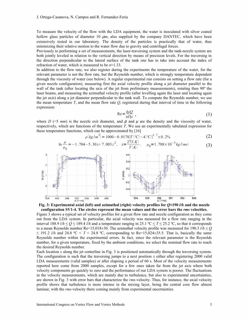
Fig. 2 : Sketch of the LDA beams crossing at the nozzle exit for axial velocity measurements, showing the distance d between the horizontal plane, where both the axial and azimuthal velocity

component are measured, and the nozzle exit (not on scale: note that d is just 1.5 mm, much smaller than the nozzle exit diameter, which is 5 mm.)

International Congress on Vortex Flow and Vortex Methods 2

J. Ortega-Casanova, N. Campos and R. Fernandez-Feria

To measure the velocity of the flow with the LDA equipment, the water is inoculated with silver coated hollow glass particles of diameter 10 µm, also supplied by the company DANTEC, which have been extensively tested in our laboratory. The density of the particles is practically that of water, thus minimizing their relative motion to the water flow due to gravity and centrifugal forces.Previously to performing a set of measurements, the laser-traversing system and the tank-nozzle system are both jointly leveled in relation to the vertical direction by means of precision levels. For the traversing in the direction perpendicular to the lateral surface of the tank one has to take into account the index of refraction of water, which is measured to be n≈1.33.In addition to the flow rate, we also register during the experiments the temperature of the water, for the relevant parameter is not the flow rate, but the Reynolds number, which is strongly temperature dependent through the viscosity of water (see below). A regular experimental run consists on setting a flow rate (for a given nozzle configuration), measuring first the axial velocity profile along a jet diameter parallel to the wall of the tank (after locating the axis of the jet from preliminary measurements), rotating then 90º the laser beams, and measuring the azimuthal velocity profile (after levelling again the laser and locating again the jet axis) along a jet diameter perpendicular to the tank wall. To compute the Reynolds number, we use the mean temperature T, and the mean flow rate Q, registered during that interval of time in the following expression:

Re=4ρQπDμ , (1)

where D (=5 mm) is the nozzle exit diameter, and ρ and μ are the density and the viscosity of water, respectively, which are functions of the temperature T. We use an experimentally tabulated expression for these temperature functions, which can be approximated by [16]

ρ kg /m3≃ 1000−0. 0178∣T ºC −4 ºC ∣1 .7±0. 2% (2)

lnμμ0

≃−1. 704−5. 30 z+ 7.003 z2 , z=273 K

T K , μ0=1. 788×10−3 kg / ms (3)

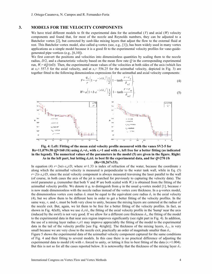
Fig. 3: Experimental axial (left) and azimuthal (right) velocity profiles for Q≈190 l/h and the nozzle configuration SV1-4. The circles represent the mean values and the error bars the rms velocities.

Figure 3 shows a typical set of velocity profiles for a given flow rate and nozzle configuration as they come out from the LDA system. In particular, the axial velocity was measured for a flow rate ranging in the interval 188.9 l/h ≤ Q ≤ 189.4 l/h and a temperature ranging in 25.1 ºC ≤ T ≤ 25.2 ºC, so that it corresponds to a mean Reynolds number Re=15,018±30. The azimuthal velocity profile was measured for 190.3 l/h ≤ Q ≤ 191.2 l/h and 24.8 ºC < T < 24.8 ºC, corresponding to Re=15,024±35.5. That is, basically the same Reynolds number within the experimental errors. In fact, since the relevant parameter is the Reynolds number, for a given temperature, fixed by the ambient conditions, we select the nominal flow rate to reach the desired Reynolds number.Each location x along the jet centerline in Fig. 3 is positioned automatically through the traversing system. The configuration is such that the traversing jumps to a next position x either after registering 2000 valid LDA measurements (valid samples) or after elapsing a period of 60 s. Most of the velocity measurements reported here come from 2000 samples, except for a few ones taken far from the jet axis where both velocity components go quickly to zero and the performance of our LDA system is poorer. The fluctuations in the velocity measurements, which are mainly due to turbulence, but also to experimental uncertainties, are shown in Fig. 3 with error bars that characterize the rms-velocity. Thus, for instance, the axial velocity profile shows that turbulence is more intense in the mixing layer, being the central core flow almost laminar, with the rms-velocity there coming mainly from experimental uncertainties.

International Congress on Vortex Flow and Vortex Methods 3

J. Ortega-Casanova, N. Campos and R. Fernandez-Feria

3. MODELS FOR THE VELOCITY COMPONENTSWe have tried different models to fit the experimental data for the azimuthal (V) and axial (W) velocity components and found that, for most of the nozzle and Reynolds numbers, they can be adjusted to a Batchelor vortex [2], but corrected by tanh-like mixing layers that adjust the flow to the external fluid at rest. This Batchelor vortex model, also called q-vortex (see, e.g., [1]), has been widely used in many vortex applications as a simple model because it is a good fit to the experimental velocity profiles for vane-guide-generated pipe vortices (e.g., [6,10]).We first convert the positions and velocities into dimensionless quantities by scaling them to the nozzle radius, D/2, and a characteristic velocity based on the mean flow rate Q in the corresponding experimental run, Wc=4Q/(πD). Then, the experimental mean values of the velocities at both sides of the axis (which lies at xa≈ 557.5 for the axial velocity, and at xa≈ 556.25 for the azimuthal velocity, depicted in Fig. 3) are together fitted to the following dimensionless expressions for the azimuthal and axial velocity components:

V=qv

r1−e

−r /δ v 2

12 1−tanh

r−rv

δv1

, (4)

W=a 1+b e−r/δ w

2

12 1− tanh

r−rw

δw1

. (5)

Fig. 4: Left: Fitting of the mean axial velocity profile measured with the vanes SV2-5 for Re=11,079±38 (Q≈160 l/h) using δw=δv, with rw=1 and with rw left free for a better fitting (as indicated in the legend). The numerical values of the parameters in the model (5) are given in the figure. Right:

As in the left part, but letting δw≠δv to best fit the experimental data, and for Q≈270 l/h (Re=18,267±33).

In equation (4) r=2n(x-xa)/D, where n≈1.33 is index of refraction of the water, because the coordinate x along which the azimuthal velocity is measured is perpendicular to the water tank wall, while in Eq. (5) r=2(x-xa)/D, since the axial velocity component is always measured traversing the laser parallel to the wall (of course, in both cases the axis of the jet is searched for previously to capturing the velocity data). The swirl parameter qv (remember that both V and W are both scaled with Wc) is obtained from the fitting of the azimuthal velocity profile. We denote it qv to distinguish from q in the usual q-vortex model [1], because r is now made dimensionless with the nozzle radius instead of the vortex core thickness. In a q-vortex model, the dimensionless vortex core radius δv must be equal to the equivalent core radius δw in the axial velocity (4), but we allow them to be different here in order to get a better fitting of the velocity profiles. In the same way, rv and rw must be both very close to unity, because the mixing layers are centered at the radius of the nozzle exit. But, again, we let them to be free for a better fitting of the velocity profiles. In fact, as shown in Fig. 4(left), when we use δw≠δv, the fitting of the axial velocity profile in the 'hump' near the axis (induced by the swirl) is not very good. If we allow for a different core thickness δw, the fitting of the model to the experimental data in that near axis region improves significantly (see right part in Fig. 4). In addition, the use of a mixing layer radius rw≠1 may improve appreciably the fitting of the model to the experimental data in the tail of the velocity profile [see Fig. 4(right)]. The thickness of the mixing layers, δw1, is very small because we are very close to the nozzle exit, practically an order of magnitude smaller than δw.Figure 5 shows the experimental data of the azimuthal velocity component captured for the same conditions of Fig. 4 and their fitting to several models. In this case there is no practical difference of adjusting the experimental data to model (4) with rv forced to unity, or letting it free to best fitting of the data (rv=1.004). But this is not so for all the cases reported below. It is noteworthy that the thickness of the mixing layer δv1

International Congress on Vortex Flow and Vortex Methods 4

J. Ortega-Casanova, N. Campos and R. Fernandez-Feria

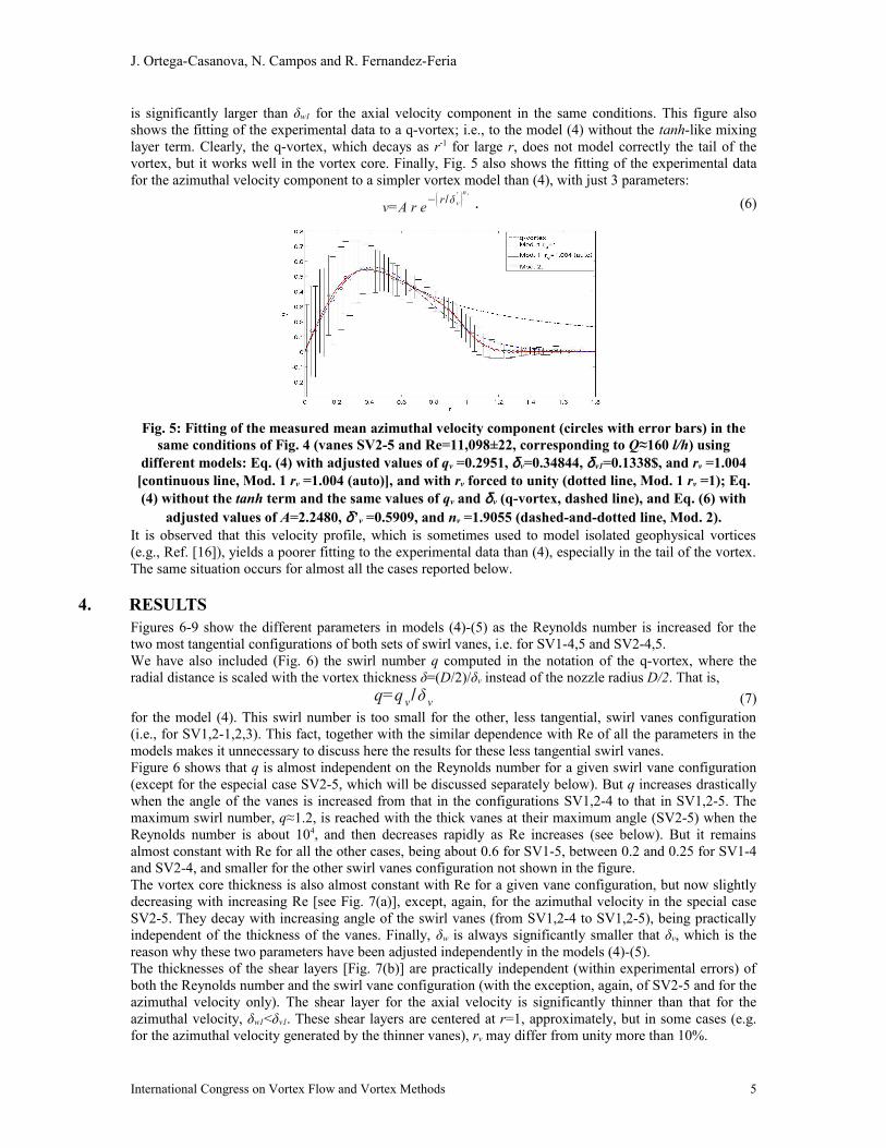
is significantly larger than δw1 for the axial velocity component in the same conditions. This figure also shows the fitting of the experimental data to a q-vortex; i.e., to the model (4) without the tanh-like mixing layer term. Clearly, the q-vortex, which decays as r-1 for large r, does not model correctly the tail of the vortex, but it works well in the vortex core. Finally, Fig. 5 also shows the fitting of the experimental data for the azimuthal velocity component to a simpler vortex model than (4), with just 3 parameters:

v=A r e− r/δ v

' n v

. (6)

Fig. 5: Fitting of the measured mean azimuthal velocity component (circles with error bars) in the same conditions of Fig. 4 (vanes SV2-5 and Re=11,098±22, corresponding to Q≈160 l/h) using

different models: Eq. (4) with adjusted values of qv =0.2951, δ v=0.34844, δ v1=0.1338$, and rv =1.004 [continuous line, Mod. 1 rv =1.004 (auto)], and with rv forced to unity (dotted line, Mod. 1 rv =1); Eq. (4) without the tanh term and the same values of qv and δ v (q-vortex, dashed line), and Eq. (6) with

adjusted values of A=2.2480, δ’v =0.5909, and nv =1.9055 (dashed-and-dotted line, Mod. 2).It is observed that this velocity profile, which is sometimes used to model isolated geophysical vortices (e.g., Ref. [16]), yields a poorer fitting to the experimental data than (4), especially in the tail of the vortex. The same situation occurs for almost all the cases reported below.

4. RESULTSFigures 6-9 show the different parameters in models (4)-(5) as the Reynolds number is increased for the two most tangential configurations of both sets of swirl vanes, i.e. for SV1-4,5 and SV2-4,5.We have also included (Fig. 6) the swirl number q computed in the notation of the q-vortex, where the radial distance is scaled with the vortex thickness δ=(D/2)/δv instead of the nozzle radius D/2. That is,

q=qv/δ v (7)for the model (4). This swirl number is too small for the other, less tangential, swirl vanes configuration (i.e., for SV1,2-1,2,3). This fact, together with the similar dependence with Re of all the parameters in the models makes it unnecessary to discuss here the results for these less tangential swirl vanes.Figure 6 shows that q is almost independent on the Reynolds number for a given swirl vane configuration (except for the especial case SV2-5, which will be discussed separately below). But q increases drastically when the angle of the vanes is increased from that in the configurations SV1,2-4 to that in SV1,2-5. The maximum swirl number, q≈1.2, is reached with the thick vanes at their maximum angle (SV2-5) when the Reynolds number is about 104, and then decreases rapidly as Re increases (see below). But it remains almost constant with Re for all the other cases, being about 0.6 for SV1-5, between 0.2 and 0.25 for SV1-4 and SV2-4, and smaller for the other swirl vanes configuration not shown in the figure.The vortex core thickness is also almost constant with Re for a given vane configuration, but now slightly decreasing with increasing Re [see Fig. 7(a)], except, again, for the azimuthal velocity in the special case SV2-5. They decay with increasing angle of the swirl vanes (from SV1,2-4 to SV1,2-5), being practically independent of the thickness of the vanes. Finally, δw is always significantly smaller that δv, which is the reason why these two parameters have been adjusted independently in the models (4)-(5).The thicknesses of the shear layers [Fig. 7(b)] are practically independent (within experimental errors) of both the Reynolds number and the swirl vane configuration (with the exception, again, of SV2-5 and for the azimuthal velocity only). The shear layer for the axial velocity is significantly thinner than that for the azimuthal velocity, δw1<δv1. These shear layers are centered at r=1, approximately, but in some cases (e.g. for the azimuthal velocity generated by the thinner vanes), rv may differ from unity more than 10%.

International Congress on Vortex Flow and Vortex Methods 5

J. Ortega-Casanova, N. Campos and R. Fernandez-Feria

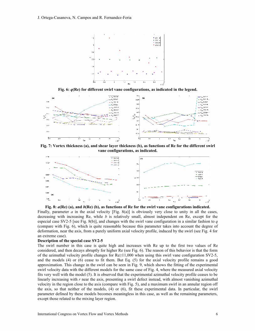
Fig. 6: q(Re) for different swirl vane configurations, as indicated in the legend.

Fig. 7: Vortex thickness (a), and shear layer thickness (b), as functions of Re for the different swirl vane configurations, as indicated.

Fig. 8: a(Re) (a), and b(Re) (b), as functions of Re for the swirl vane configurations indicated.Finally, parameter a in the axial velocity [Fig. 8(a)] is obviously very close to unity in all the cases, decreasing with increasing Re, while b is relatively small, almost independent on Re, except for the especial case SV2-5 [see Fig. 8(b)], and changes with the swirl vane configuration in a similar fashion to q (compare with Fig. 6), which is quite reasonable because this parameter takes into account the degree of deformation, near the axis, from a purely uniform axial velocity profile, induced by the swirl (see Fig. 4 for an extreme case).Description of the special case SV2-5The swirl number in this case is quite high and increases with Re up to the first two values of Re considered, and then decays abruptly for higher Re (see Fig. 6). The reason of this behavior is that the form of the azimuthal velocity profile changes for Re≥11,000 when using this swirl vane configuration SV2-5, and the models (4) or (6) cease to fit them. But Eq. (5) for the axial velocity profile remains a good approximation. This change in the swirl can be seen in Fig. 9, which shows the fitting of the experimental swirl velocity data with the different models for the same case of Fig. 4, where the measured axial velocity fits very well with the model (5). It is observed that the experimental azimuthal velocity profile ceases to be linearly increasing with r near the axis, presenting a swirl defect instead, with almost vanishing azimuthal velocity in the region close to the axis (compare with Fig. 5), and a maximum swirl in an annular region off the axis, so that neither of the models, (4) or (6), fit these experimental data. In particular, the swirl parameter defined by these models becomes meaningless in this case, as well as the remaining parameters, except those related to the mixing layer region.

International Congress on Vortex Flow and Vortex Methods 6

J. Ortega-Casanova, N. Campos and R. Fernandez-Feria

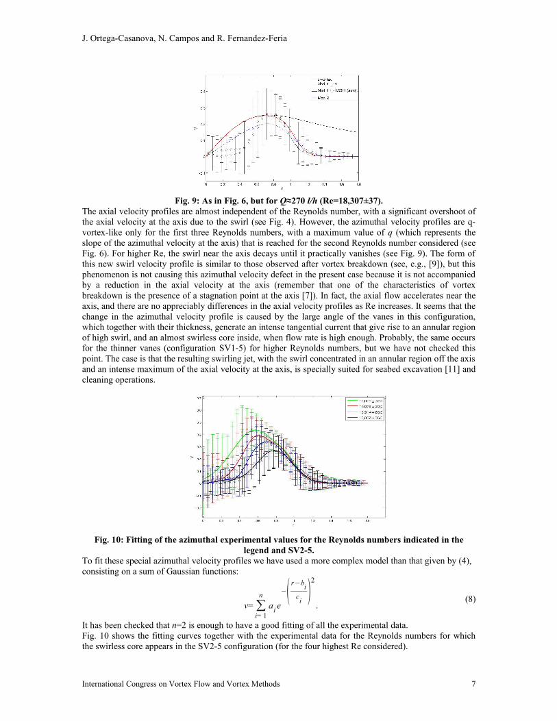
Fig. 9: As in Fig. 6, but for Q≈270 l/h (Re=18,307±37).The axial velocity profiles are almost independent of the Reynolds number, with a significant overshoot of the axial velocity at the axis due to the swirl (see Fig. 4). However, the azimuthal velocity profiles are q-vortex-like only for the first three Reynolds numbers, with a maximum value of q (which represents the slope of the azimuthal velocity at the axis) that is reached for the second Reynolds number considered (see Fig. 6). For higher Re, the swirl near the axis decays until it practically vanishes (see Fig. 9). The form of this new swirl velocity profile is similar to those observed after vortex breakdown (see, e.g., [9]), but this phenomenon is not causing this azimuthal velocity defect in the present case because it is not accompanied by a reduction in the axial velocity at the axis (remember that one of the characteristics of vortex breakdown is the presence of a stagnation point at the axis [7]). In fact, the axial flow accelerates near the axis, and there are no appreciably differences in the axial velocity profiles as Re increases. It seems that the change in the azimuthal velocity profile is caused by the large angle of the vanes in this configuration, which together with their thickness, generate an intense tangential current that give rise to an annular region of high swirl, and an almost swirless core inside, when flow rate is high enough. Probably, the same occurs for the thinner vanes (configuration SV1-5) for higher Reynolds numbers, but we have not checked this point. The case is that the resulting swirling jet, with the swirl concentrated in an annular region off the axis and an intense maximum of the axial velocity at the axis, is specially suited for seabed excavation [11] and cleaning operations.

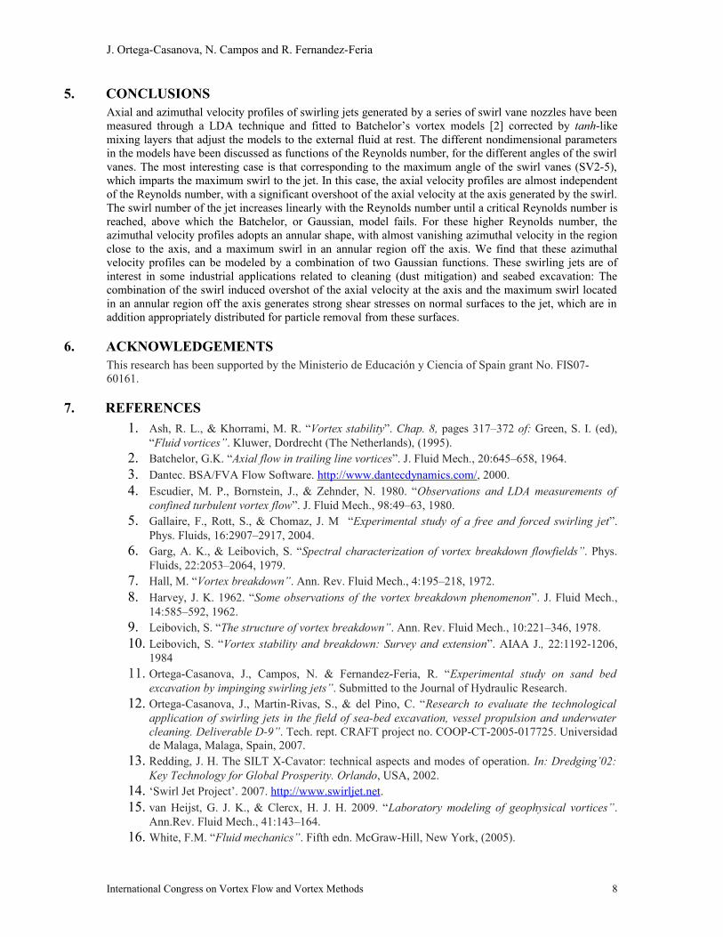
Fig. 10: Fitting of the azimuthal experimental values for the Reynolds numbers indicated in the legend and SV2-5.

To fit these special azimuthal velocity profiles we have used a more complex model than that given by (4), consisting on a sum of Gaussian functions:

v=∑i= 1

n

ai e

−r−b

ici

2

. (8)

It has been checked that n=2 is enough to have a good fitting of all the experimental data.Fig. 10 shows the fitting curves together with the experimental data for the Reynolds numbers for which the swirless core appears in the SV2-5 configuration (for the four highest Re considered).

International Congress on Vortex Flow and Vortex Methods 7

J. Ortega-Casanova, N. Campos and R. Fernandez-Feria

5. CONCLUSIONSAxial and azimuthal velocity profiles of swirling jets generated by a series of swirl vane nozzles have been measured through a LDA technique and fitted to Batchelor’s vortex models [2] corrected by tanh-like mixing layers that adjust the models to the external fluid at rest. The different nondimensional parameters in the models have been discussed as functions of the Reynolds number, for the different angles of the swirl vanes. The most interesting case is that corresponding to the maximum angle of the swirl vanes (SV2-5), which imparts the maximum swirl to the jet. In this case, the axial velocity profiles are almost independent of the Reynolds number, with a significant overshoot of the axial velocity at the axis generated by the swirl. The swirl number of the jet increases linearly with the Reynolds number until a critical Reynolds number is reached, above which the Batchelor, or Gaussian, model fails. For these higher Reynolds number, the azimuthal velocity profiles adopts an annular shape, with almost vanishing azimuthal velocity in the region close to the axis, and a maximum swirl in an annular region off the axis. We find that these azimuthal velocity profiles can be modeled by a combination of two Gaussian functions. These swirling jets are of interest in some industrial applications related to cleaning (dust mitigation) and seabed excavation: The combination of the swirl induced overshot of the axial velocity at the axis and the maximum swirl located in an annular region off the axis generates strong shear stresses on normal surfaces to the jet, which are in addition appropriately distributed for particle removal from these surfaces.

6. ACKNOWLEDGEMENTSThis research has been supported by the Ministerio de Educación y Ciencia of Spain grant No. FIS07-60161.

7. REFERENCES

1. Ash, R. L., & Khorrami, M. R. “Vortex stability”. Chap. 8, pages 317–372 of: Green, S. I. (ed), “Fluid vortices”. Kluwer, Dordrecht (The Netherlands), (1995).

2. Batchelor, G.K. “Axial flow in trailing line vortices”. J. Fluid Mech., 20:645–658, 1964.3. Dantec. BSA/FVA Flow Software. http://www.dantecdynamics.com/, 2000.4. Escudier, M. P., Bornstein, J., & Zehnder, N. 1980. “Observations and LDA measurements of

confined turbulent vortex flow”. J. Fluid Mech., 98:49–63, 1980.5. Gallaire, F., Rott, S., & Chomaz, J. M “Experimental study of a free and forced swirling jet”.

Phys. Fluids, 16:2907–2917, 2004. 6. Garg, A. K., & Leibovich, S. “Spectral characterization of vortex breakdown flowfields”. Phys.

Fluids, 22:2053–2064, 1979.7. Hall, M. “Vortex breakdown”. Ann. Rev. Fluid Mech., 4:195–218, 1972.8. Harvey, J. K. 1962. “Some observations of the vortex breakdown phenomenon”. J. Fluid Mech.,

14:585–592, 1962.9. Leibovich, S. “The structure of vortex breakdown”. Ann. Rev. Fluid Mech., 10:221–346, 1978.10. Leibovich, S. “Vortex stability and breakdown: Survey and extension”. AIAA J., 22:1192-1206,

198411. Ortega-Casanova, J., Campos, N. & Fernandez-Feria, R. “Experimental study on sand bed

excavation by impinging swirling jets”. Submitted to the Journal of Hydraulic Research.12. Ortega-Casanova, J., Martin-Rivas, S., & del Pino, C. “Research to evaluate the technological

application of swirling jets in the field of sea-bed excavation, vessel propulsion and underwater cleaning. Deliverable D-9”. Tech. rept. CRAFT project no. COOP-CT-2005-017725. Universidad de Malaga, Malaga, Spain, 2007.

13. Redding, J. H. The SILT X-Cavator: technical aspects and modes of operation. In: Dredging’02: Key Technology for Global Prosperity. Orlando, USA, 2002.

14. ‘Swirl Jet Project’. 2007. http://www.swirljet.net.15. van Heijst, G. J. K., & Clercx, H. J. H. 2009. “Laboratory modeling of geophysical vortices”.

Ann.Rev. Fluid Mech., 41:143–164.16. White, F.M. “Fluid mechanics”. Fifth edn. McGraw-Hill, New York, (2005).

International Congress on Vortex Flow and Vortex Methods 8