Switching Lemma for Bilinear Tests and Constant-size … · Switching Lemma for Bilinear Tests and...

Switching Lemma for Bilinear Tests and

Constant-size NIZK Proofs for Linear Subspaces ∗

Charanjit S. Jutla

IBM T. J. Watson Research Center

Yorktown Heights, NY 10598, USA

Arnab Roy

Fujitsu Laboratories of America

Sunnyvale, CA 94085, USA

May 12, 2018

Abstract

We state a switching lemma for tests on adversarial responses involving bilinear pairingsin hard groups, where the tester can effectively switch the randomness used in the test frombeing given to the adversary at the outset to being chosen after the adversary commits itsresponse. The switching lemma can be based on any k-linear hardness assumptions on oneof the groups. In particular, this enables convenient information theoretic arguments in theconstruction of sequence of games proving security of cryptographic schemes, mimicking proofsand constructions in the random oracle model.

As an immediate application, we show that the computationally-sound quasi-adaptive NIZKproofs for linear subspaces that were recently introduced [JR13] can be further shortened toconstant -size proofs, independent of the number of witnesses and equations. In particular, un-der the XDH assumption, a length n vector of group elements can be proven to belong to asubspace of rank t with a quasi-adaptive NIZK proof consisting of just a single group element.Similar quasi-adaptive aggregation of proofs is also shown for Groth-Sahai NIZK proofs of lin-ear multi-scalar multiplication equations, as well as linear pairing-product equations (equationswithout any quadratic terms).

Keywords: NIZK, bilinear pairings, quasi-adaptive, Groth-Sahai, Random Oracle, IBE, CCA2.

1 Introduction

Testing pairing equations in bilinear groups is a fundamental component of numerous cryptographicschemes spanning public key encryption schemes, signatures, zero knowledge proofs and so on.We state and prove a switching lemma for testing pairing equations in bilinear groups, wherean adversary is given some random group elements from one of the groups, and the pairing test(of equality and/or inequality) is performed on adversary’s output and the same random groupelements. We show that the tester can replace the random group elements in the test with a newset of fresh random group elements, effectively mimicking the behavior of a random oracle. Thisswitching lemma can be based on any k-linear hardness assumptions on one of the groups. This notonly enables convenient information theoretic arguments in the construction of sequence of games

∗An extended abstract of this paper [JR14] appears in the proceedings of CRYPTO 2014. This is the full version.

1

proving security of cryptographic schemes, but also allows more efficient protocols reminiscent ofthe Fiat-Shamir paradigm using random oracles [FS87].

Fiat-Shamir paradigm is best illustrated by the conversion of 3-round sigma protocol [Dam]for proof of knowledge (PoK) of discrete logarithms to a random oracle based NIZK. Consider anexample where the prover is trying to prove possession of the discrete logarithm x of a public valuegx. In the first round the prover commits to a random value r by sending gr. In response, theverifier generates a fresh random value c and sends to the prover. The prover then responds withr + cx. This constitutes an honest verifier zero-knowledge PoK. In transforming this to a NIZK,a public random oracle H is used and the prover just transmits (gr, r +H(gr, gx) · x). Essentiallythe random oracle induces the effect of a ‘fresh’ randomness that can be used for verification andis not under any effective control of the prover. In this paper we create an analogous effect inthe standard model using the hardness of k-linear problems (such as DDH and DLIN) in bilineargroups. We show that even if the random testing values are public and hence known to the prover,during verification one can switch to freshly generated testing values with negligible change in theprobability of success of the verification.

As an immediate application, we show that the computationally-sound quasi-adaptive NIZK(QA-NIZK) proofs for linear subspaces that we recently introduced in [JR13] can be further short-ened to constant-size proofs, independent of the number of variables and equations. In [JR13],it was shown that for languages that are linear subspaces of vector spaces of the bilinear groups,one can obtain more efficient computationally-sound NIZK proofs compared to [GS08] in a slightlydifferent quasi-adaptive setting, which suffices for many cryptographic applications. In the quasi-adaptive setting, a class of parametrized languages {Lρ} is considered, parametrized by ρ, and theCRS generator is allowed to generate the CRS based on the language parameter ρ. However, theCRS simulator in the zero-knowledge setting is required to be a single efficient algorithm that worksfor the whole parametrized class or probability distributions of languages, by taking the parameteras input. This property was referred to as uniform simulation.

The main idea underlying the construction in [JR13] can be summarized as follows. Considerthe language Lρ (over a cyclic group G of order q, in additive notation) defined as

Lρ ={

〈l1, l2, l 3〉 ∈ G3 | ∃x1, x2 ∈ Zq : l1 = x1 · g, l2 = x2 · f , l3 = (x1 + x2) · h

}

where ρdef= (g, f , h) is the parameter defining the language. Suppose that the CRS can be set to be

a basis for the null-space L⊥ρ of the language Lρ. Then, just pairing a potential language candidate

with L⊥ρ and testing for all-zero suffices to prove that the candidate is in Lρ, as the null-space of L⊥ρ

is just Lρ. However, efficiently computing null-spaces in hard bilinear groups is itself hard. Thus,an efficient CRS simulator cannot generate L⊥ρ . However, it was shown that it suffices to give asCRS a (hiding) commitment that is computationally indistinguishable from a binding commitmentto L⊥ρ .

Our contributions. Utilizing the switching lemma, for n equations in t variables, our computa-tionally-sound quasi-adaptive NIZK proofs for linear subspaces require only k group elements underthe k-linear decisional assumption [HK07, Sha07]. Thus, under the XDH1 assumption for bilineargroups, our proofs require only one group element. In contrast, the Groth-Sahai system requires

1 XDH is the assumption that DDH is hard in one of the pairing groups. Also note that DDH is same as thek-linear assumption for k = 1.

2

Table 1: Comparison with Groth-Sahai, Jutla-Roy (2013) and Schnorr-NIZKs for Linear Subspaces.Parameter t is the number of unknowns and n is the dimension of the vector space, i.e. the numberof equations. See text for recent independent work.

XDH DLINProof CRS #Pairings Proof CRS #Pairings

Groth-Sahai n+ 2t 4 2n(t+ 2) 2n+ 3t 9 3n(t + 3)Jutla-Roy ’13 n− t 2t(n− t) + 2 (n− t)(t + 2) 2n− 2t 4t(n − t) + 3 2(n− t)(t + 2)Schnorr (RO) t+ 2 − − − − −

This paper 1 n+ t + 1 n+ 1 2 2(n+ t+ 2) 2(n+ 2)

Table 2: Comparison with (1) Groth-Sahai for n number of linear Scalar Multiplication Equations:~y ·~aj + ~bj ·~x = uj , with j ∈ [1, n], ~y ∈ Zq

s, ~x ∈ Gt and uj ∈ G. and (2) Groth-Sahai for n number

of linear Pairing Product Equations: e(~y, ~aj) + e(~bj, ~x) = uj , with j ∈ [1, n], ~y ∈ Gs, ~x ∈ G

t anduj ∈ GT .

DLIN Linear Multi-Scalar and Linear Pairing-ProductProof CRS #Pairings

Groth-Sahai 3(s + t) + 9n 9 9n(s+ t+ 3) + n

This paper 3(s + t) + 18 9 + 4n 18(s + t+ 3) + n

(n+2t) group elements and our previous system required (n− t) group elements. Similarly, underthe decisional linear assumption (DLIN), our proofs require only 2 group elements, whereas theGroth-Sahai system requires (2n + 3t) group elements and our previous system required (2n− 2t)group elements. These parameters are summarized in Table 1. While our CRS size grows linearlywith n, the number of pairing operations is competitive and could be significantly less comparedto earlier schemes for appropriate n and t.

Note that Schnorr proofs of multiple equations in the random oracle model can also be combinedinto a proof consisting of only two group elements (by taking random linear combinations employingthe random oracle), but it still requires commitments to all the variables. Thus, our proofs are evenshorter than Schnorr proofs. On the other hand, Schnorr proofs are proof of knowledge (as opposedto ours or Groth-Sahai), and can be somewhat faster to verify as they only use exponentiationinstead of pairings. We also show that proofs of multiple linear scalar-multiplication equations,as well as multiple linear pairing product equations (i.e. without any quadratic terms) can beaggregated into a single proof in the Groth-Sahai system. This can lead to significant shortening ofproofs of multiple linear pairing product equations. The comparisons are tabulated in Table 2. Weremark that this is in contrast to the batching of Groth-Sahai proof verification [BFI+10], wherethe proofs were not aggregated, but multiple pairing equations were batched together during theverification step. We can use similar batching techniques to improve the verification step; therefore,we skip taking these optimizations into consideration. A recent work [LPJY14] has also obtainedconstant-size QA-NIZK proofs under DLIN (but not under XDH). While our proofs are marginallyshorter (2 against 3 in DLIN), they additionally show constant-size unbounded simulation-soundQA-NIZK proofs.

While the cryptographic literature is replete with applications using NIZK proofs of algebraiclanguages over bilinear groups, and many examples were given in [JR13] involving NIZK proofs oflinear subspaces, we focus on two particular cases where aggregation of proofs of linear subspaces

3

lead to interesting results. We consider a construction of [CCS09] to convert key-dependent message(KDM) CPA secure encryption scheme [BHHO08] into a KDM-CCA2 secure scheme which involvedproving O(N) linear equations, where N is the security parameter. With our aggregation of proofs,the size of this proof (in the quasi-adaptive setting) is reduced to just 2 group elements (under theDLIN assumption) from the earlier O(N) sized quasi-adaptive proofs and Groth-Sahai proofs. It isalso easy to see that the quasi-adaptive setting for proving the NIZK suffices, as is the case for mostapplications. As another application we reduce the size of the publicly-verifiable CCA2-IBE schemeobtained in [JR13] by another group element to just five group elements plus a tag. This makes itshorter than the highly-optimized CCA2-IBE scheme obtained using the [CHK04] paradigm fromhierarchical-IBE (HIBE) and in addition is publicly-verifiable.

Organization of the paper. We begin the rest of the paper with the switching lemma for bilineartests in hard groups in Section 2. We recall the quasi-adaptive NIZK definitions in Section 3 anddevelop constant-size quasi-adaptive NIZKs for linear subspaces in Section 4. In Section 5, we applyour switching lemma to aggregate Groth-Sahai NIZKs. Finally, we provide application examplesin Section 6. We defer detailed proofs, formal descriptions and a summary of standard hardnessassumptions that we use to the Appendix.

2 Switching Lemma for Bilinear Tests in Hard Groups

Notations. Consider bilinear groups G1 and G2 with pairing e to a target group GT , all of primeorder q, and random generators g1 ∈ G1 and g2 ∈ G2. Let 01, 02 and 0T be the identity elementsin the three groups G1,G2 and GT respectively. We will use additive notation for group operations,with G1,G2 and GT viewed as Zq-vector spaces. The scalar product by Zq elements naturallyextends to vectors and matrices of group elements. The pairing operation also naturally extends tovectors of elements (by summation) and correspondingly to matrices of elements. Column vectorswill be denoted by an arrow over the letter, e.g. ~r for (column) vector of Zq elements, and ~d as

(column) vector of group elements. Thus, e(~f⊤, ~h) =

∑

i e(fi,hi). However, sometimes we will userow interpretation for vectors. When not clear from context, we will disambiguate by indicatingthe matrix dimensions in the superscript.

Switching Lemma Usage Example. We demonstrate the usage of the Switching Lemma byway of a toy example. Suppose we are given three elements g, f (= a ·g),h(= b ·g) in the group G1

and we need a proof system, not necessarily ZK, for tuples of the form (x · g, x · f , x · h). Towardsthat end, suppose the following CRS is published: ((ar1+ br2) ·g2,−r1 ·g2,−r2 ·g2). So the pairingtest e(x · g, (ar1 + br2) · g2) + e(x · f ,−r1 · g2) + e(x · h,−r2 · g2) = 0T , satisfies completeness, i.e.,it holds for valid tuples.

However, how do we know that it is sound? A look at the pairing equation shows that there isa fair degree of freedom to satisfy it, without being a valid tuple. So we definitely have to resort toa computational hardness assumption to argue soundness. This is where we invoke the switchinglemma, which is based on a hardness assumption. Thus even though we publish a CRS that usesr1, r2, during verification we can switch them with fresh r′1, r

′2 chosen randomly and independently.

This means if a candidate tuple (l1, l 2, l3) satisfies the original test with a certain probability,then it also satisfies the switched test: e(l 1, (ar

′1+br

′2)·g2)+e(l 2,−r

′1 ·g2)+e(l 3,−r

′2 ·g2) = 0T with

4

almost the same probability. Rearranging, we get: r′1 · e(a · l1 − l2,g2) + r′2 · e(b · l1 − l3,g2) = 0T .Now, observe that the r′1, r

′2 were chosen after the tuple was given. So with high probability, both

of e(a · l1 − l2,g2) and e(b · l1 − l3,g2) must be 0T . Therefore, l2 = a · l1 and l3 = b · l1, thusproving soundness.

Another way to look at this is that we produced a single CRS by random linear combination ofCRS’es to prove the individual languages {(x · g, x · f ) | x ∈ Zq} and {(x · g, x · h) | x ∈ Zq}. Sincethe combined CRS is given to the adversary, we cannot resort to information-theoretic argumentsto separate the individual equations. However with the switching lemma in play, the separationfollows.

Switching Lemma Intuition. First consider the asymmetric bilinear group setting, where DDHholds in each individual group, and there is no easy isomorphism from G1 to G2 and vice-versa. If anAdversary A is given two random group elements, say r1, r2, from G2, then one would like to claimthat it is highly improbable for A to produce non-zero f1, f2 in G1 such that e(f1, r1)+e(f2, r2) = 0T .First, note that if the groups were symmetric, then this is easy to achieve by setting f1 = r2 andf2 = −r1. But, since we are in the asymmetric setting, the improbability is proven under DDHholding for G2 as follows: We will show that an adversary A that can produce a non-zero f1, f2satisfying the above pairing equation can be used to produce an adversary B that can break DDH.So, given a DDH challenge, g2, x ·g2, y ·g2 and h which is either xy ·g2 or z ·g2, adversary B passesg2, x ·g2 to A (note they are random and independent). Since A produces non-zero f1, f2 such thate(f1,g2)+ e(f2, x · g2) = 0T , it follows that f1 = −x · f2. Then comparing e(f1, y · g2) with −e(f2,h)allows B to distinguish the two versions of h.

Surprisingly, a similar claim holds when the adversary A is given an arbitrary long, say lengthn vector ~r of random group elements from G2, and A is required to produce a length n vector ~f

(from G1) such that e(~f⊤,~r) = 0T . This is proven using a hybrid argument, and for that purpose

it is useful to restate the above claim of improbability as a switching lemma: Given r1, r2, if anadversary has probability ∆ success in producing non-zero f1, f2 such that e(f1, r1) + e(f2, r2) = 0T ,then the probability of e(f1, r

′1)+ e(f2, r

′2) = 0T holding is also negligibly close to ∆, where r′1, r

′2 are

chosen after A commits f1, f2.

Moving on to the symmetric bilinear groups, and assuming that the k-linear (commonly calledDLIN for 2-linear) assumption holds for the groups, one can show that if A is now given k inde-pendent pairs of random group elements, then it is highly improbable for A to produce non-zerof1, f2 such that the above pairing test holds for all k pairs (with the same f1, f2). Again, a switchinglemma variant is more useful for proving the general lemma for n-vectors. Further, the reductionto the k-linear assumption is achieved by embedding the k-linear challenge in a single pairing testwhich is a random linear combination of the k pairing tests.

We now state the switching lemma in its full generality and later remark on interesting specialcases.

Lemma 1 (Switching Lemma) Let D be an arbitrary efficiently samplable distribution over n×m matrices from Zq. For any PPT adversary A producing a vector of n elements from group G1,let ∆A be the following probability

Pr

R$←− G

m×k2 , C

n×m ← D, ~fn×1← A(g1,g2,R,C) :

~f 6= ~0n×11 and e

(

~f⊤,C · R

)

= ~01×kT

5

Then, under the k-linear assumption for group G2, the following probability is negligibly close to∆A.

Pr

R$←− G

m×k2 , C

n×m ← D, ~fn×1← A(g1,g2,R,C), R

′ $←− G

m×k2 :

~f 6= ~0n×11 and e

(

~f⊤,C · R′

)

= ~01×kT

The absolute value of the difference in the probabilities is bounded by m · adv(klin).

Remarks. If we assume that the distribution D overwhelmingly produces full ranked matrices,then observe that the later probability is information theoretically close to 0. Hence we can state:

Pr

R$←− G

m×k2 , Cn×m ← D, ~f

n×1← A(g1,g2,R,C) :

~f 6= ~0n×11 and e

(

~f⊤,C · R

)

= ~01×kT

≈k−linear 0

If, however, D produces singular matrices non-negligibly often, then there is an efficient adver-

sary that can induce the event ~f 6= ~01 and e(~f⊤,C · R) = ~0T . The switching lemma still stands

since the same adversary can induce the event ~f 6= ~01 and e(

~f⊤,C · R′

)

= ~0T just as easily.

Although the presence of the C matrix is not strictly essential for the settings that we considerin this paper, we leave it in this form for generalizations to groups where the scalar field or ring isnot easily invertible.

Instead of using the k-linear assumption directly, we use a related assumption which we call thek-lifted linear assumption and is implied by the k-linear assumption with a perfect reduction.

Definition 2 (k-lifted linear assumption) For a constant k ≥ 1, assuming a generation algo-

rithm G that outputs a tuple (q,G) such that G is of prime order q and has a generator g$←− G, the

k-lifted linear assumption asserts that it is computationally infeasible to distinguish between

Tuple0 =

(

b1 · g, · · · , bk · g, r1 · g, · · · , rk · g, b1s1 · g, · · · , bksk · g,

(

n∑

i=1

risi

)

· g

)

andTuple1 = (b1 · g, · · · , bk · g, r1 · g, · · · , rk · g, b1s1 · g, · · · , bksk · g, sk+1 · g) .

More formally, for all PPT adversaries A there exists a negligible function ν() such that

∣

∣

∣

∣

∣

Pr[(q,G)← G(1m);g$←− G; b1, ..., bk, r1, ..., rk , s1, ..., sk+1

$←− Zq : A(Tuple0) = 1]−

Pr[(q,G)← G(1m);g$←− G; b1, ..., bk, r1, ..., rk, s1, ..., sk+1

$←− Zq : A(Tuple1) = 1]

∣

∣

∣

∣

∣

< ν(m)

It is worth noting that the k-linear assumption is a variant of the k-lifted linear assumption withall r1, ..., rk equal to one. But the following shows that the k-lifted linear assumption is weaker.

Theorem 3 (k-linear assumption ⇒ k-lifted linear assumption) The k-linear assumption im-plies the k-lifted linear assumption. Moreover, the advantage of a k-lifted linear adversary is upperbounded by the maximum advantage of a k-linear adversary.

6

Proof: Suppose we are given a k-linear instance (b1 ·g, ..., bk ·g, g, b1s1 ·g, ..., bksk ·g, χ), whereχ is either (s1+...+sk)·g or random. We will now efficiently construct a k-lifted linear instance fromthis k-linear instance, thus showing a randomized reduction from the k-linear challenge problem tothe k-lifted linear challenge problem.

Choose u1, ..., uk$←− Zq. Implicitly set ri = biui+1. Thus ri ·g = ui · (bi · g)+g. The ri ·g’s are

independently random wrt the bi · g’s due to the ui’s. Now consider χ′ =∑k

i=1 [ui · (bisi · g)] + χ.

In the case where χ = (s1 + ... + sk) · g, this is equal to∑k

i=1 [ui · (bisi · g)] + (s1 + ... + sk) · g =∑k

i=1 [ui · (bisi · g) + si · g] =∑k

i=1 [risi · g]. In the case where χ is random, χ′ is random. Hencethe following tuple is a k-lifted linear Tuple0 if χ is from a real k-linear distribution and is ak-lifted linear Tuple1 if χ is from a fake k-linear distribution:

(

b1 · g, · · · , bk · g, r1 · g, · · · , rk · g, b1s1 · g, · · · , bksk · g,χ′)

�

Proof: (of Lemma 1) When m ≤ k, the lemma follows information-theoretically (although theproof for m > k also works for this case) by noting that in this case R will have rank m with highprobability. Now we focus on the case that m > k. Consider the following inductive hypothesis(over j):

Pr

R$←− G

m×k2 , Cn×m ← D, ~f

n×1← A(g1,g2,R,C), R

′ $←− G

m×k2 :

~f 6= ~0n×1

and e(

~f⊤,C · R′′

)

= ~01×kT

differs from ∆A by at most j ·adv(klin), where R′′ has the first (m− j) rows same as first (m− j)rows of R and the last j rows same as the last j rows of R′. In the base case, i.e., when j = 0, thisis same as the hypothesis (antecedent) in the lemma, and when j = m, this induction hypothesisis same as the claim (consequent) in the lemma. Thus, we just need to prove the induction step.

For an adversary A, suppose the difference in the two probabilities corresponding to (inductionhypothesis for) j = t and j = t + 1 be δ. More precisely, denote the probability for adversary Acorresponding to j = t by ∆t. Thus, we are supposing that |∆t −∆t+1| ≥ δ. Using A as a blackbox we wlll demonstrate an adversary S that will have advantage at least (negligibly close to) δ tobreak the k-lifted linear assumption.

So, let a k-lifted linear challenger produce: (b1 · g2, · · · , bk · g2, r1 · g2,..., rk · g2, b1s1 · g2,...,bksk · g2, χ) in the group G2, where χ is either (

∑ni=1 risi) · g2 or random. Note that bi, ri and si

are chosen randomly and independently by the challenger.

Let vectors ~r and~s be defined component-wise as (~r)i = ri ·g2 and (~s)i = si, respectively. Definethe k by k matrix B as the diagonal matrix with the i-th diagonal element set to bi. Further, letB = B · g2.

S samples Cn×m ← D, and chooses g1 at random. It next samples an (m− t− 1) by k matrixR1 at random from Zq (i.e. all elements of the matrix chosen randomly and independently fromZq). It sets R1 = R1 ·B. It further samples a t by k matrix R2 at random from G2 (i.e. all elementschosen randomly and independently from G2). Finally S sets R to be the rows of R1, the row ~r⊤

and the rows of R2 combined (in that order) to form an m by k matrix. Observe that all of R’sentries are independently random. The adversary A is then given g1, g2, R and C. The adversaryA in response produces ~f. Now, S first checks that ~f is non-zero. It then chooses another t byk matrix R2 at random from Zq and sets R2 = R2 · B. Noting that S has access to B ·~s · g2, S

7

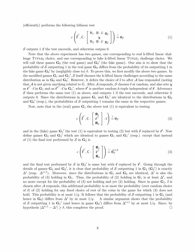
(efficiently) performs the following bilinear test

e

~f⊤,C ·

R1 · B ·~s · g2χ

R2 · B ·~s · g2

?= 0T (1)

S outputs 1 if the test succeeds, and otherwise outpus 0.

Note that the above experiment has two games, one corresponding to real k-lifted linear chal-lenge Tuple0 choice, and one corresponding to fake k-lifted linear Tuple1 challenge choice. Wewill call these games G0 (the real game) and G0

′ (the fake game). Our aim is to show that theprobability of S outputting 1 in the real game G0 differs from the probability of its outputting 1 inthe fake game G0

′ by (negligibly close to) δ. To prove this, we first modify the above two games. Inthe modified games G1 and G1

′, S itself chooses the k-lifted linear challenges according to the samedistribution as in G0 and G0

′. However, it defers the choice of ~s to after A has responded (notingthat A is not given anything related to~s). After A responds, S chooses~s at random, and also sets χas ~r⊤ ·~s in G1 and as ~r′⊤ ·~s in G1

′, where ~r′ is another random k-tuple independent of ~r. AdversaryS then performs the same test (1) as above, and outputs 1 if the test succeeds, and otherwise itoutputs 0. Since the distributions in games G1 and G1

′ are identical to the distributions in G0

and G0′ (resp.), the probabilities of S outputting 1 remains the same in the respective games.

Now, note that in the (real) game G1 the above test (1) is equivalent to testing

e

~f⊤,C ·

R1

~r⊤

R2

·~s

?= 0T (2)

and in the (fake) game G1′ the test (1) is equivalent to testing (2) but with ~r replaced by ~r′. Now

define games G2 and G2′ which are identical to games G1 and G1

′ (resp.) except that insteadof (1) the final test performed by S in G2 is

e

~f⊤,C ·

R1

~r⊤

R2

?= ~0

1×kT (3)

and the final test performed by S in G2′ is same but with ~r replaced by ~r′. Going through the

details of games G2 and G2′, it is clear that probability of S outputting 1 in G2 (G2

′) is exactly∆t (resp. ∆t+1). Moreover, since the distributions in G1 and G2 are identical, ∆t is also theprobability of (3) holding in G1. Thus, the probability of (2) holding in G1 is at least ∆t, andno more except for the probability of (3) not holding and yet (2) holding. Since in game G1, ~s ischosen after A responds, this additional probability is at most the probability (over random choiceof ~s) of (2) holding for any fixed choice of rest of the coins in the game for which (3) does nothold. This probability is at most 1/q. It follows that the probability of S outputting 1 in G1 (andhence in G0) differs from ∆t by at most 1/q. A similar argument shows that the probabilityof S outputting 1 in G1

′ (and hence in game G0′) differs from ∆t+1 by at most 1/q. Since, by

hypothesis |∆t+1 −∆t| ≥ δ, this completes the proof. �

8

3 Quasi-Adaptive NIZK Proofs

We recall here the definitions from [JR13] and provide a summary. Instead of considering NIZKproofs for a (witness-) relation R, the authors consider Quasi-Adaptive NIZK proofs for a probabilitydistribution D on a collection of (witness-) relations R = {Rρ}. The quasi-adaptiveness allows forthe common reference string (CRS) to be set based on Rρ after the latter has been chosen accordingto D. However the simulator generating the CRS (in the simulation world) is required to be a singleprobabilistic polynomial time algorithm that works for the whole collection of relations R.

To be more precise, they consider ensemble {Dλ} of distributions on collection of relations Rλ,where each Dλ specifies a probability distribution on Rλ = {Rλ,ρ}. When λ is clear from contextit can be dropped. Since in the quasi-adaptive setting the CRS could depend on the relation, anassociated parameter language Lpar is considered such that a member of this language is enoughto characterize a particular relation, and this language member is provided to the CRS generator.

A tuple of algorithms (K0,K1,P,V) is called a QA-NIZK proof system for witness-relationsRλ = {Rρ} with parameters sampled from a distribution D over associated parameter languageLpar, if there exists a probabilistic polynomial time simulator (S1,S2), such that for all non-uniformPPT adversaries A1,A2,A3 we have:

Quasi-Adaptive Completeness:

Pr[λ← K0(1m); ρ← Dλ;ψ ← K1(λ, ρ); (x,w) ← A1(λ, ρ, ψ);

π ← P(ψ, x,w) : V(ψ, x, π) = 1 if Rρ(x,w)] = 1

Quasi-Adaptive Soundness:

Pr[λ← K0(1m); ρ← Dλ;ψ ← K1(λ, ρ);

(x, π)← A2(λ, ρ, ψ) : V(ψ, x, π) = 1 and ¬(∃w : Rρ(x,w))] ≈ 0

Quasi-Adaptive Zero-Knowledge:

Pr[λ← K0(1m); ρ← Dλ;ψ ← K1(λ, ρ) : A

P(ψ,·,·)3 (λ, ρ, ψ) = 1] ≈

Pr[λ← K0(1m); ρ← Dλ; (ψ, τ)← S1(λ, ρ) : A

S(ψ,τ,·,·)3 (λ, ρ, ψ) = 1],

where S(ψ, τ, x,w) = S2(ψ, τ, x) for (x,w) ∈ Rρ and both oracles (i.e. P and S) output failureif (x,w) 6∈ Rρ.

Note that ψ is the CRS in the above definitions.

3.1 Stronger QA-NIZK Definition

We now consider a stronger definition of QA-NIZK where all the three notions above are potentiallystronger, as the Adversary will be given more power. We remark that a related stronger notionwas considered earlier in [GHR15, LPJY15], as we discuss below.

Instead of considering probability distributions on witness-relations, we now define QA-NIZKfor a language of witness-relations. Each witness-relation in the language is defined by a parameter

9

that comes from a parameter language Lpar. The QA-NIZK parameter language Lpar also has itsown witness relation Rpar. A parameter ρ is in Lpar iff there exists a θ such that (ρ, θ) ∈ Rpar.

A tuple of algorithms (K0,K1,P,V) is called a QA-NIZK proof system for witness-relationsRλ = {Rρ} with parameters from a associated parameter language Lpar which has its own witness-relation Rpar, if there exists a probabilistic polynomial time simulator (S1,S2), such that for allnon-uniform PPT adversaries A0,A1,A2,A3 we have:

Quasi-Adaptive Completeness:

Pr[λ← K0(1m); (ρ, θ, σ)← A0(λ);ψ ← K1(λ, ρ); (x,w) ← A1(λ, ρ, ψ, σ);

π ← P(ψ, x,w) : V(ψ, x, π) = 1 if (Rρ(x,w) and Rpar(ρ, θ))] = 1

Strong Quasi-Adaptive Soundness:

Pr[λ← K0(1m); (ρ, θ, σ)← A0(λ);ψ ← K1(λ, ρ);

(x, π)← A2(λ, ρ, ψ) : V(ψ, x, π) = 1 and ¬(∃w : Rρ(x,w)) and Rpar(ρ, θ)] ≈ 0

Quasi-Adaptive Zero-Knowledge:

Pr[λ← K0(1m); (ρ, θ, σ)← A0(λ);ψ ← K1(λ, ρ) : A

P(ψ,·,·)3 (λ, ρ, ψ, σ) = 1 and Rpar(ρ, θ)] ≈

Pr[λ← K0(1m); (ρ, θ, σ)← A0(λ); (ψ, τ) ← S1(λ, ρ) : A

S(ψ,τ,·,·)3 (λ, ρ, ψ, σ) = 1 and Rpar(ρ, θ)],

where S(ψ, τ, x,w) = S2(ψ, τ, x) for (x,w) ∈ Rρ and both oracles (i.e. P and S) output failureif (x,w) 6∈ Rρ.

Remark 1. We will refer to such QA-NIZK as QA-NIZK for parameterized languages asopposed to the earlier definition which we will call QA-NIZK for distribution of parameterizedlanguages. This definition of QA-NIZK is stronger than the previous definition if D (over Lpar)is efficiently witness-samplable. In that case, we can just consider A0 to be the efficient witness-sampler of D.

Remark 2. An alternate viewpoint was earlier taken in [GHR15, LPJY15] where for the witness-samplable distributions case, in the original definition, even if the Adversary is given witness θ ofρ after (ρ, θ) are chosen according to D, the QA-NIZK remains sound. For example, in the case oflinear-subspace languages, the language parameter A which is a matrix of group elements definesthe language for which the NIZK is being considered. Then, even if discrete-log of components ofA, i.e. A, are given to the adversary, it still cannot produce a non-language member that passesthe verification test. However, the definition above in this sub-section is even more general thanconsidered in [GHR15, LPJY15].

Remark 3. For most applications it suffices to consider definitions of completeness and zero-knowledge such that the Adversary A0 need only produce ρ as long as it is in Lpar.

Remark 4. Various other constructions of QA-NIZK were given in recent years [LPJY14, ABP15,GHR15], some even guaranteeing simulation-soundness [LPJY14, ABP15, KW15, JR15, LPJY15].All of these constructions that worked for efficiently witness-samplable distributions, also satisfythe above stronger definition.

10

4 Aggregating Quasi-Adaptive Proofs of Linear Subspaces

We summarize the linear-subspace QA-NIZK setting of [JR13] here and refer the reader to thatpaper for details.

Linear Subspace Languages. We consider languages that are linear subspaces of vectors ofG1 elements. In other words, the languages we are interested in can be characterized as languagesparametrized by A as below:

LA = {~x⊤ ·A ∈ Gn1 | ~x ∈ Zq

t}, where A is a t× n matrix of G1 elements.

Here A is an element of the associated parameter language Llin, which is all t × n matrices ofG1 elements. The parameter language Llin also has a corresponding witness relation Rlin, wherethe witness is a matrix of Zq elements : Rlin(A,A) iff A = A · g1.

Robust and Efficiently Witness-Samplable Distributions. Let the t×n dimensional matrixA be chosen according to a distribution D on Llin. The distribution D is called robust if withprobability close to one the left-most t columns of A are full-ranked. A distribution D on Llin iscalled efficiently witness-samplable if there is a probabilistic polynomial time algorithm such that itoutputs a pair of matrices (A,A) that satisfy the relation Rlin (i.e., Rlin(A,A) holds), and furtherthe resulting distribution of the output A is same as D. For example, the uniform distribution onLlin is efficiently witness-samplable, by first picking A at random, and then computing A.

QA-NIZK Construction. We now describe a computationally sound quasi-adaptive NIZK(K0,K1,P,V) for linear subspace languages {LA} with parameters sampled from a robust andefficiently witness-samplable distribution D over the associated parameter language Llin. As aconceptual starting point, we first develop a construction which has k2 element proofs, demonstrat-ing a single application of the Switching Lemma. Later, we give a k element construction whichlinearly combines the first construction proofs and uses an additional layer of Switching Lemmaapplication. Our description here is self sufficient and relates to the scheme in [JR13] in that welinearly combine proofs of multiple elements yielding constant-size proofs.

Algorithm K1: The algorithm K1 generates the CRS as follows. Let At×n be the parameter

supplied to K1. Let sdef= n − t: this is the number of equations in excess of the unknowns. It

generates a matrix Dt×k2 with all elements chosen randomly from Zq and k elements {bv}v∈[1,k]

and sk elements {riu}i∈[1,s],u∈[1,k] all chosen randomly from Zq. Define matrices Rs×k2

and Bk2×k2

component-wise as follows:

(R)i,k(u−1)+v = riu, with i ∈ [1, s], u, v ∈ [1, k].

(B)ij =

{

bv if i = j = k(u− 1) + v, with u, v ∈ [1, k]

0 if i 6= j, with i, j ∈ [1, k2]

Intuitively, the matrix R is a k times column-wise repetition of the rij’s, and if we denote

{bv}v∈[1,k] by ~b, then the diagonal matrix B is just the vector ~b repeated k times along the diagonal(i.e. Bk(u−1)+v,k(u−1)+v is bv and not bu).

11

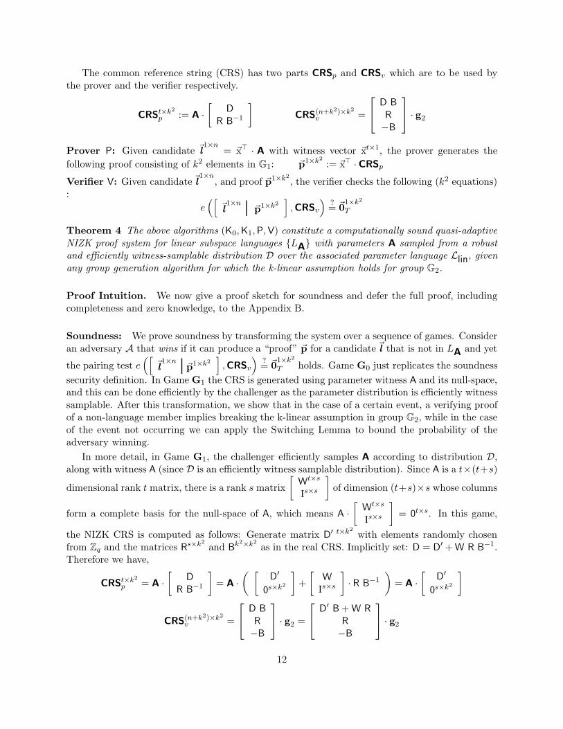
The common reference string (CRS) has two parts CRSp and CRSv which are to be used bythe prover and the verifier respectively.

CRSt×k2

p := A ·

[

D

R B−1

]

CRS(n+k2)×k2

v =

D B

R

−B

· g2

Prover P: Given candidate ~l1×n

= ~x⊤ · A with witness vector ~xt×1, the prover generates the

following proof consisting of k2 elements in G1: ~p1×k2 := ~x⊤ · CRSp

Verifier V: Given candidate ~l1×n

, and proof ~p1×k2 , the verifier checks the following (k2 equations):

e([

~l1×n

~p1×k2]

,CRSv

)

?= ~0

1×k2

T

Theorem 4 The above algorithms (K0,K1,P,V) constitute a computationally sound quasi-adaptiveNIZK proof system for linear subspace languages {LA} with parameters A sampled from a robustand efficiently witness-samplable distribution D over the associated parameter language Llin, givenany group generation algorithm for which the k-linear assumption holds for group G2.

Proof Intuition. We now give a proof sketch for soundness and defer the full proof, includingcompleteness and zero knowledge, to the Appendix B.

Soundness: We prove soundness by transforming the system over a sequence of games. Consideran adversary A that wins if it can produce a “proof” ~p for a candidate ~l that is not in LA and yet

the pairing test e([

~l1×n

~p1×k2]

,CRSv

)

?= ~0

1×k2

T holds. Game G0 just replicates the soundness

security definition. In Game G1 the CRS is generated using parameter witness A and its null-space,and this can be done efficiently by the challenger as the parameter distribution is efficiently witnesssamplable. After this transformation, we show that in the case of a certain event, a verifying proofof a non-language member implies breaking the k-linear assumption in group G2, while in the caseof the event not occurring we can apply the Switching Lemma to bound the probability of theadversary winning.

In more detail, in Game G1, the challenger efficiently samples A according to distribution D,along with witness A (since D is an efficiently witness samplable distribution). Since A is a t×(t+s)

dimensional rank t matrix, there is a rank s matrix

[

Wt×s

Is×s

]

of dimension (t+s)×s whose columns

form a complete basis for the null-space of A, which means A ·

[

Wt×s

Is×s

]

= 0t×s. In this game,

the NIZK CRS is computed as follows: Generate matrix D′ t×k2 with elements randomly chosen

from Zq and the matrices Rs×k2

and Bk2×k2 as in the real CRS. Implicitly set: D = D

′ +W R B−1.

Therefore we have,

CRSt×k2

p = A ·

[

D

R B−1

]

= A ·

( [

D′

0s×k2

]

+

[

W

Is×s

]

· R B−1

)

= A ·

[

D′

0s×k2

]

CRS(n+k2)×k2v =

D B

R

−B

· g2 =

D′B+W R

R

−B

· g2

12

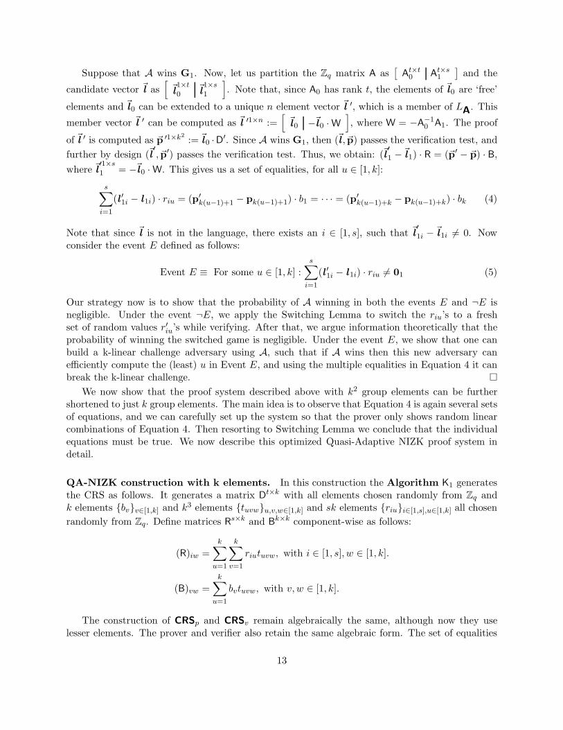
Suppose that A wins G1. Now, let us partition the Zq matrix A as[

At×t0 A

t×s1

]

and the

candidate vector ~l as[

~l1×t

0~l1×s

1

]

. Note that, since A0 has rank t, the elements of ~l0 are ‘free’

elements and ~l0 can be extended to a unique n element vector ~l ′, which is a member of LA. This

member vector ~l ′ can be computed as ~l ′1×n :=[

~l0 −~l0 ·W]

, where W = −A−10 A1. The proof

of ~l ′ is computed as ~p ′1×k2

:= ~l0 ·D′. Since A wins G1, then (~l , ~p) passes the verification test, and

further by design (~l′, ~p′) passes the verification test. Thus, we obtain: (~l

′

1 −~l1) · R = (~p′ − ~p) · B,

where ~l′1×s

1 = −~l0 ·W. This gives us a set of equalities, for all u ∈ [1, k]:

s∑

i=1

(l ′1i − l1i) · riu = (p′k(u−1)+1 − pk(u−1)+1) · b1 = · · · = (p′k(u−1)+k − pk(u−1)+k) · bk (4)

Note that since ~l is not in the language, there exists an i ∈ [1, s], such that ~l′

1i −~l1i 6= 0. Now

consider the event E defined as follows:

Event E ≡ For some u ∈ [1, k] :s∑

i=1

(l ′1i − l1i) · riu 6= 01 (5)

Our strategy now is to show that the probability of A winning in both the events E and ¬E isnegligible. Under the event ¬E, we apply the Switching Lemma to switch the riu’s to a freshset of random values r′iu’s while verifying. After that, we argue information theoretically that theprobability of winning the switched game is negligible. Under the event E, we show that one canbuild a k-linear challenge adversary using A, such that if A wins then this new adversary canefficiently compute the (least) u in Event E, and using the multiple equalities in Equation 4 it canbreak the k-linear challenge. �

We now show that the proof system described above with k2 group elements can be furthershortened to just k group elements. The main idea is to observe that Equation 4 is again several setsof equations, and we can carefully set up the system so that the prover only shows random linearcombinations of Equation 4. Then resorting to Switching Lemma we conclude that the individualequations must be true. We now describe this optimized Quasi-Adaptive NIZK proof system indetail.

QA-NIZK construction with k elements. In this construction the Algorithm K1 generatesthe CRS as follows. It generates a matrix D

t×k with all elements chosen randomly from Zq andk elements {bv}v∈[1,k] and k

3 elements {tuvw}u,v,w∈[1,k] and sk elements {riu}i∈[1,s],u∈[1,k] all chosen

randomly from Zq. Define matrices Rs×k and Bk×k component-wise as follows:

(R)iw =

k∑

u=1

k∑

v=1

riutuvw, with i ∈ [1, s], w ∈ [1, k].

(B)vw =k∑

u=1

bvtuvw, with v,w ∈ [1, k].

The construction of CRSp and CRSv remain algebraically the same, although now they uselesser elements. The prover and verifier also retain the same algebraic form. The set of equalities

13

for this construction corresponding to the equation (~l′

1 −~l1) · R = (~p′ − ~p) · B, is for all w ∈ [1, k]:

s∑

i=1

[

(l ′1i − l1i) ·

(

k∑

u=1

k∑

v=1

riutuvw

)]

−

k∑

v=1

[

(p′v − pv) ·

(

k∑

u=1

bvtuvw

)]

= 01 (6)

Rearranging, we get for all w ∈ [1, k]:

k∑

u=1

k∑

v=1

[

tuvw

(

s∑

i=1

[

(l ′1i − l1i) · riu]

− (p′v − pv) · bv

)]

= 01 (7)

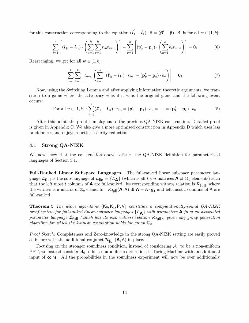
Now, using the Switching Lemma and after applying information theoretic arguments, we tran-sition to a game where the adversary wins if it wins the original game and the following eventoccurs:

For all u ∈ [1, k] :s∑

i=1

(l ′1i − l1i) · riu = (p′1 − p1) · b1 = · · · = (p′k − pk) · bk (8)

After this point, the proof is analogous to the previous QA-NIZK construction. Detailed proofis given in Appendix C. We also give a more optimized construction in Appendix D which uses lessrandomness and enjoys a better security reduction.

4.1 Strong QA-NIZK

We now show that the construction above satisfies the QA-NIZK definition for parameterizedlanguages of Section 3.1.

Full-Ranked Linear Subspace Languages. The full-ranked linear subspace parameter lan-guage Lfull is the sub-language of Llin = {LA} (which is all t×n matrices A of G1 elements) suchthat the left most t columns of A are full-ranked. Its corresponding witness relation is Rfull, wherethe witness is a matrix of Zq elements : Rfull(A,A) iff A = A · g1 and left-most t columns of A arefull-ranked.

Theorem 5 The above algorithms (K0,K1,P,V) constitute a computationally-sound QA-NIZKproof system for full-ranked linear-subspace languages {LA} with parameters A from an associatedparameter language Lfull (which has its own witness relation Rfull), given any group generationalgorithm for which the k-linear assumption holds for group G2.

Proof Sketch: Completeness and Zero-knowledge in the strong QA-NIZK setting are easily provedas before with the additional conjunct Rfull(A,A) in place.

Focusing on the stronger soundness condition, instead of considering A0 to be a non-uniformPPT, we instead consider A0 to be a non-uniform deterministic Turing Machine with an additionalinput of coins. All the probabilities in the soundness experiment will now be over additionally

14

choosing coins uniformly at random. Then,

Pr[λ← K0(1m); (ρ, θ, σ)← A0(λ, coins);ψ ← K1(λ, ρ);

(x, π)← A2(λ, ρ, ψ) : V(ψ, x, π) = 1 ∧ Rpar(ρ, θ) ∧ ¬(∃w : Rρ(x,w))]

=∑

c

Pr[λ← K0(1m); (ρ, θ, σ)← A0(λ, coins);ψ ← K1(λ, ρ);

(x, π)← A2(λ, ρ, ψ) : V(ψ, x, π) = 1 ∧ Rpar(ρ, θ) ∧ ¬(∃w : Rρ(x,w)) ∧ coins = c]

=∑

c

Pr[coins = c] ∗ Pr[λ← K0(1m); (ρ, θ, σ)← A0(λ, c);ψ ← K1(λ, ρ);

(x, π)← A2(λ, ρ, ψ) : V(ψ, x, π) = 1 ∧ Rpar(ρ, θ) ∧ ¬(∃w : Rρ(x,w))]

We will show2 that there is an ǫ, such that for every c,

Pr[λ← K0(1m); (ρ, θ, σ)← A0(λ, c);ψ ← K1(λ, ρ);

(x, π)← A2(λ, ρ, ψ) : V(ψ, x, π) = 1 ∧ Rpar(ρ, θ) ∧ ¬(∃w : Rρ(x,w))] < ǫ,

so that the above sum is also upper-bounded by ǫ.

To this end, consider an adversary (A0,A2) that wins if it can produce (A,A) in Lfull, and a

“proof” ~p for a candidate ~l that is not in LA and yet the pairing test holds.

Now, fix a c. In game G1, the challenger uses the given λ and the deterministic A0, with coins

set to c, to generate (A,A). Since Rfull is efficiently computable, the challenger terminates if (A,A)is not in Lfull (note, rank of columns of A can be computed efficiently). The probability of theAdversary winning remains the same. The rest of the proof continues as before, yielding an upperbound on Adversary’s success for this fixed c to be (2k+s) ·adv(klin)+O(1)/q (note, the constantimplicit in O(1)/q is also same for all c).

5 Aggregating Groth-Sahai Proofs

We show that proofs of multiple linear scalar-multiplication equations, as well as multiple linearpairing product equations can be aggregated into a single proof in the Groth-Sahai system. Wewill focus on describing the aggregation for the scalar-multiplication equations, as the results forthe linear pairing product equations are obtained in almost an identical manner.

Consider bilinear groups G1 and G2 with pairing e into a third group GT . Consider equationsof the type

n∑

i=1

yi · ai +

m∑

i=1

bi · xi = t1 (9)

where the variables yi are to take values in Zq, the variables xi are to take values in G1. Theconstants ai are in G1, and scalar constants bi are in Zq. Moreover, t1 is in G1.

When the bilinear group is symmetric, i.e. G1 = G2, and under the DLIN assumption, theGroth-Sahai NIZK proof of the above equation requires commitments to the variables, each com-mitment being of size three group elements (for both yi or xi). In addition it requires a proof of

2More precisely by Appendix D, for the QA-NIZK construction above with k elements, ǫ < (2k+ s) · adv(klin) +O(1)/q.

15

nine group elements. When there are multiple equations of the above kind in the same variables,the commitments to the variables remain the same, but each equation requires nine group elements.In other words, if there are m+ n variables and k equations, the full proof of the k equations hassize 3 · (m+ n) + 9k group elements.

We will now show that in the quasi-adaptive setting, the full proof of the k equations can beobtained with size 3 · (m + n) + 9 group elements. We first describe how the proof is done in theGroth-Sahai system, and then we will point out the relevant changes. The proofs and commitmentsactually belong to the Zq-module G

3 (where G = G1 = G2).

We will write these groups in additive notation, and the bilinear pairing operation e(A,B)written in infix notation as A⊗B, with the pairing operation defining a tensor product G⊗G overZq. Without loss of generality (see e.g. A2.2 in [Eis95]), we can assume that GT = G⊗G. Further,this naturally extends to a tensor product G3

⊗G3. One can also define a tensor product Zq ⊗G,

but since G is a Zq-module, this tensor product is just G.

Let ι1 : Zq → G3, ι2 : G→ G

3, p1 : G3 → Zq, p2 : G

3 → G be group homomorphisms s.t. ι1 ◦p1,and ι2 ◦ p2 are identity maps in Zq and G resp. Note that the maps ι1 and ι2 naturally define agroup homomorphism ιT from Zq ⊗ G (= G) to G

3⊗G

3, and similarly p1 and p2 define a grouphomomorphism pT from G

3⊗G

3 to Zq ⊗G (= G).

The NIZK common reference string (CRS) consists of three elements from G3, i.e. u1,u2,u3 ∈

G3. They are chosen as follows: u1 = (α · g,O,g), and u2 = (O, β · g,g), and u3 = ru1 + su2, for

random α, β, r, s ∈ Zq, and random g ∈ G\O. This real-world CRS ~u is sometimes also referred toas the binding CRS.

The map ι2(Z) is just (O,O,Z), and p2(Z1,Z2,Z3) = Z3 − α−1Z1 − β−1Z2, which showsthat ι2 ◦ p2 is an identity map. It also shows that p2(u1) = p2(u2) = p2(u3) = O. Now, thecommitments to elements Z in G are made by picking r1, r2, r3 at random from Zq, and settingc2(Z) = ι2(Z) + r1u1 + r2u2 + r3u3. Thus, p2(c2(Z)) = Z, and hence the name binding CRS.

The map ι1(z) is ι2(z · g), and hence commitment to z ∈ Zq is c1(z) = c2(z · g).

For equations of the form (9) , i.e. ~y · ~a + ~b · ~x = t1, a proof ~π (along with commitmentsto variables) is obtained by setting ~π = S⊤ι2(~a) + R⊤ι1(~b) + ~θ, where R is the matrix of rows(r1, r2, r3), coming from c2(xi), one for each committed variable xi, and S is the matrix of rows(r1, r2, r3), coming from c1(yi), one for each committed variable yi. Note, ~π is vector of three G

3

elements. The vector ~θ is set to be a random linear combination of Hi~u , where Hi are finitelymany matrices, and form a basis for the solutions to ~u •H~u = 0. It turns out that these matricesHi are independent of the ZK simulator trapdoors α and β.

Let “•” denote the dot product of vectors of elements from G3 and G

3 w.r.t. product ⊗ . Thecommitments ~c1, ~c2 and the proof are verified by the following equation:

ι1(~b) • ~c2 + ~c1 • ι2(~a) = ι1(1) • ι2(t1) + ~u • ~π.

Quasi-Adaptive Aggregation. In the quasi-adaptive setting [JR13], the NIZK CRS is allowedto depend on the language parameters, but with the further requirement that the ZK simulationbe uniform. In the above context, the language parameters are ~a and ~b. Note t1 is not a languageparameter, as it is a quantity produced by the prover.

So, let there be k equations in the same variables, with the j-th equation being

~y · ~aj + ~bj · ~x = tj1 (10)

16

In the above setting the prover produces k proofs, ~πj . We would like the prover to give a randomlinear combination of these proofs, where the randomness is fixed in the CRS setup. In the DLINsetting, we need two different linear combinations. Thus, let the CRS generator choose two randomZq-vectors ~ρ and ~ψ. The prover is required to produce ~πρ =

∑

j∈[1,k] ρj ·~πj and ~πψ =

∑

j∈[1,k] ψj ·~πj .

To be able to do so, the prover needs∑

j ρj · ι2(~aj),∑

j ρj · ι1(~bj) (and similar terms using ψj). The

~θ terms in the proofs need not be linearly combined, and the prover can just add one such term toeach of ~πρ and ~πψ, as its purpose is only to allow zero-knowledge simulation (i.e. witness hiding).The CRS generator can certainly produce these elements and give them as part of the CRS. TheCRS generator also needs to give as part of the verification CRS the terms 〈ι1(ρj)〉j and 〈ι1(ψj)〉j .In order to apply the switching lemma, we show in the proof of the theorem below that if ~aj areefficiently witness samplable, then the CRS generator can also simulate this verification CRS givenρj · g and ψj · g.

The verification is now done as follows:

(∑

j

ρj · ι1(~bj)) • ~c2 + ~c1 • (

∑

j

ρj · ι2(~aj)) =

∑

j

(ι1(ρj) • ι2(tj1)) + ~u • ~πρ (11)

(∑

j

ψj · ι1(~bj)) • ~c2 + ~c1 • (

∑

j

ψj · ι2(~aj)) =

∑

j

(ι1(ψj) • ι2(tj1)) + ~u • ~πψ (12)

Theorem 6 The above system constitutes a computationally-sound quasi-adaptive NIZK proof sys-tem for equations (10) with parameters 〈~aj〉j, 〈~b

j〉j , whenever 〈~aj〉j are chosen according to anefficiently witness-samplable distribution, and given any group generation algorithm for which theDLIN assumption holds.

Proof of the theorem can be found in Appendix E. Since Groth-Sahai proofs of more generalequations (involving quadratic terms) require pairing of adversarially supplied commitments witheach other, the switching lemma is not directly applicable. It remains an open problem to aggregatesuch NIZK proofs.

6 Extensions and Applications

Tags. We extend the system of Section 4 to include tags mirroring [JR13]. The tags are elementsof Zq, are included as part of the proof and are used as part of the defining equations of the language.We still get k element proofs based on the k-linear assumption. Details are in Appendix F.

KDM-CCA2 Encryption [CCS09]. In the paper [CCS09], the authors construct a public keyencryption scheme simultaneously secure against key dependent chosen plaintext (KDM) and adap-tive chosen ciphertext attacks (CCA2). They apply a Naor-Yung “double encryption” paradigm tocombine any KDM-CPA secure scheme with any IND-CCA2 secure scheme along with an appropri-ate NIZK proof, to obtain a KDM-CCA2 secure scheme. In a particular construction, they obtainshort ciphertexts by combining the KDM-CPA secure scheme of [BHHO08] with the IND-CCA2scheme of [CS98], along with a Groth-Sahai NIZK proof. We show that the NIZK proof requiredin this construction can be considerably shortened. We defer the reader to [CCS09] for details ofthe scheme, and just describe the equations to be proved here. Consider bilinear groups G1 andG2 in which the K-linear and L-linear assumptions hold, respectively.

17

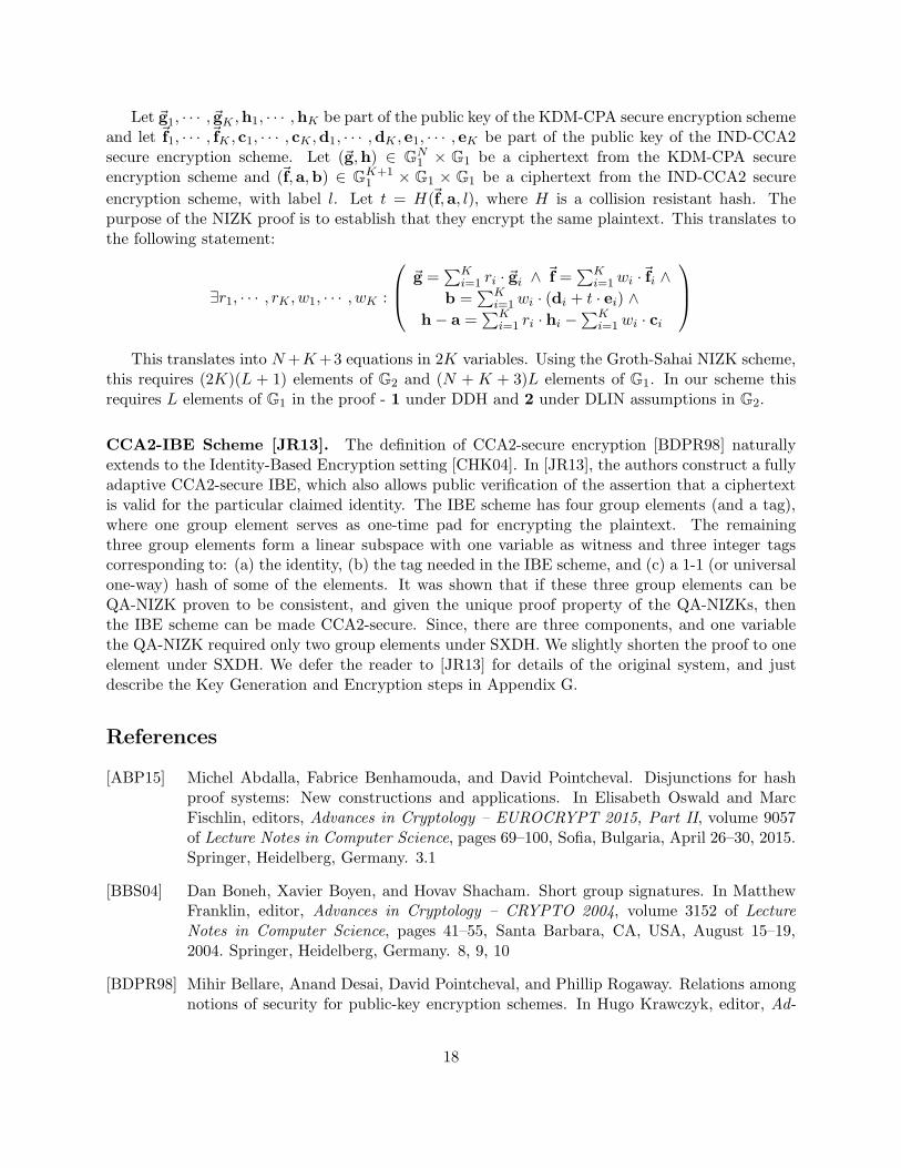
Let ~g1, · · · , ~gK ,h1, · · · ,hK be part of the public key of the KDM-CPA secure encryption schemeand let ~f1, · · · ,~fK , c1, · · · , cK ,d1, · · · ,dK , e1, · · · , eK be part of the public key of the IND-CCA2secure encryption scheme. Let (~g,h) ∈ G

N1 × G1 be a ciphertext from the KDM-CPA secure

encryption scheme and (~f,a,b) ∈ GK+11 × G1 × G1 be a ciphertext from the IND-CCA2 secure

encryption scheme, with label l. Let t = H(~f,a, l), where H is a collision resistant hash. Thepurpose of the NIZK proof is to establish that they encrypt the same plaintext. This translates tothe following statement:

∃r1, · · · , rK , w1, · · · , wK :

~g =∑K

i=1 ri · ~gi ∧~f =

∑Ki=1wi ·

~fi ∧

b =∑K

i=1wi · (di + t · ei) ∧

h− a =∑K

i=1 ri · hi −∑K

i=1 wi · ci

This translates into N+K+3 equations in 2K variables. Using the Groth-Sahai NIZK scheme,this requires (2K)(L + 1) elements of G2 and (N + K + 3)L elements of G1. In our scheme thisrequires L elements of G1 in the proof - 1 under DDH and 2 under DLIN assumptions in G2.

CCA2-IBE Scheme [JR13]. The definition of CCA2-secure encryption [BDPR98] naturallyextends to the Identity-Based Encryption setting [CHK04]. In [JR13], the authors construct a fullyadaptive CCA2-secure IBE, which also allows public verification of the assertion that a ciphertextis valid for the particular claimed identity. The IBE scheme has four group elements (and a tag),where one group element serves as one-time pad for encrypting the plaintext. The remainingthree group elements form a linear subspace with one variable as witness and three integer tagscorresponding to: (a) the identity, (b) the tag needed in the IBE scheme, and (c) a 1-1 (or universalone-way) hash of some of the elements. It was shown that if these three group elements can beQA-NIZK proven to be consistent, and given the unique proof property of the QA-NIZKs, thenthe IBE scheme can be made CCA2-secure. Since, there are three components, and one variablethe QA-NIZK required only two group elements under SXDH. We slightly shorten the proof to oneelement under SXDH. We defer the reader to [JR13] for details of the original system, and justdescribe the Key Generation and Encryption steps in Appendix G.

References

[ABP15] Michel Abdalla, Fabrice Benhamouda, and David Pointcheval. Disjunctions for hashproof systems: New constructions and applications. In Elisabeth Oswald and MarcFischlin, editors, Advances in Cryptology – EUROCRYPT 2015, Part II, volume 9057of Lecture Notes in Computer Science, pages 69–100, Sofia, Bulgaria, April 26–30, 2015.Springer, Heidelberg, Germany. 3.1

[BBS04] Dan Boneh, Xavier Boyen, and Hovav Shacham. Short group signatures. In MatthewFranklin, editor, Advances in Cryptology – CRYPTO 2004, volume 3152 of LectureNotes in Computer Science, pages 41–55, Santa Barbara, CA, USA, August 15–19,2004. Springer, Heidelberg, Germany. 8, 9, 10

[BDPR98] Mihir Bellare, Anand Desai, David Pointcheval, and Phillip Rogaway. Relations amongnotions of security for public-key encryption schemes. In Hugo Krawczyk, editor, Ad-

18

vances in Cryptology – CRYPTO’98, volume 1462 of Lecture Notes in Computer Sci-ence, pages 26–45, Santa Barbara, CA, USA, August 23–27, 1998. Springer, Heidelberg,Germany. 6

[BFI+10] Olivier Blazy, Georg Fuchsbauer, Malika Izabachene, Amandine Jambert, Herve Sibert,and Damien Vergnaud. Batch Groth-Sahai. In Jianying Zhou and Moti Yung, editors,ACNS 10: 8th International Conference on Applied Cryptography and Network Security,volume 6123 of Lecture Notes in Computer Science, pages 218–235, Beijing, China,June 22–25, 2010. Springer, Heidelberg, Germany. 1

[BHHO08] Dan Boneh, Shai Halevi, Michael Hamburg, and Rafail Ostrovsky. Circular-secure en-cryption from decision Diffie-Hellman. In David Wagner, editor, Advances in Cryptology– CRYPTO 2008, volume 5157 of Lecture Notes in Computer Science, pages 108–125,Santa Barbara, CA, USA, August 17–21, 2008. Springer, Heidelberg, Germany. 1, 6

[CCS09] Jan Camenisch, Nishanth Chandran, and Victor Shoup. A public key encryption schemesecure against key dependent chosen plaintext and adaptive chosen ciphertext attacks.In Antoine Joux, editor, Advances in Cryptology – EUROCRYPT 2009, volume 5479of Lecture Notes in Computer Science, pages 351–368, Cologne, Germany, April 26–30,2009. Springer, Heidelberg, Germany. 1, 6

[CHK04] Ran Canetti, Shai Halevi, and Jonathan Katz. Chosen-ciphertext security from identity-based encryption. In Christian Cachin and Jan Camenisch, editors, Advances in Cryp-tology – EUROCRYPT 2004, volume 3027 of Lecture Notes in Computer Science, pages207–222, Interlaken, Switzerland, May 2–6, 2004. Springer, Heidelberg, Germany. 1, 6

[CS98] Ronald Cramer and Victor Shoup. A practical public key cryptosystem provably secureagainst adaptive chosen ciphertext attack. In Hugo Krawczyk, editor, Advances inCryptology – CRYPTO’98, volume 1462 of Lecture Notes in Computer Science, pages13–25, Santa Barbara, CA, USA, August 23–27, 1998. Springer, Heidelberg, Germany.6

[Dam] Ivan Damgard. On Σ protocols. http://www.daimi.au.dk/~ivan/Sigma.pdf. 1

[DH76] Whitfield Diffie and Martin E. Hellman. New directions in cryptography. IEEE Trans-actions on Information Theory, 22(6):644–654, 1976. 7

[Eis95] David Eisenbud. Commutative algebra with a view toward algebraic geometry, volume150 of Graduate Texts in Mathematics. Springer-Verlag, 1995. 5

[FS87] Amos Fiat and Adi Shamir. How to prove yourself: Practical solutions to identificationand signature problems. In Andrew M. Odlyzko, editor, Advances in Cryptology –CRYPTO’86, volume 263 of Lecture Notes in Computer Science, pages 186–194, SantaBarbara, CA, USA, August 1987. Springer, Heidelberg, Germany. 1

[GHR15] Alonso Gonzalez, Alejandro Hevia, and Carla Rafols. QA-NIZK arguments in asym-metric groups: New tools and new constructions. In Tetsu Iwata and Jung Hee Cheon,editors, Advances in Cryptology – ASIACRYPT 2015, Part I, volume 9452 of LectureNotes in Computer Science, pages 605–629, Auckland, New Zealand, November 30 –December 3, 2015. Springer, Heidelberg, Germany. 3.1

19

http://www.daimi.au.dk/~ivan/Sigma.pdf

[GS08] Jens Groth and Amit Sahai. Efficient non-interactive proof systems for bilinear groups.In Nigel P. Smart, editor, Advances in Cryptology – EUROCRYPT 2008, volume 4965of Lecture Notes in Computer Science, pages 415–432, Istanbul, Turkey, April 13–17,2008. Springer, Heidelberg, Germany. 1

[HK07] Dennis Hofheinz and Eike Kiltz. Secure hybrid encryption from weakened key encap-sulation. In Alfred Menezes, editor, Advances in Cryptology – CRYPTO 2007, volume4622 of Lecture Notes in Computer Science, pages 553–571, Santa Barbara, CA, USA,August 19–23, 2007. Springer, Heidelberg, Germany. 1, 11

[JR13] Charanjit S. Jutla and Arnab Roy. Shorter quasi-adaptive NIZK proofs for linearsubspaces. In Kazue Sako and Palash Sarkar, editors, Advances in Cryptology – ASI-ACRYPT 2013, Part I, volume 8269 of Lecture Notes in Computer Science, pages 1–20,Bengalore, India, December 1–5, 2013. Springer, Heidelberg, Germany. (document), 1,1, 3, 4, 4, 5, 6, 6, F, G

[JR14] Charanjit S. Jutla and Arnab Roy. Switching lemma for bilinear tests and constant-sizeNIZK proofs for linear subspaces. In Juan A. Garay and Rosario Gennaro, editors, Ad-vances in Cryptology – CRYPTO 2014, Part II, volume 8617 of Lecture Notes in Com-puter Science, pages 295–312, Santa Barbara, CA, USA, August 17–21, 2014. Springer,Heidelberg, Germany. ∗

[JR15] Charanjit S. Jutla and Arnab Roy. Dual-system simulation-soundness with applicationsto UC-PAKE and more. In Tetsu Iwata and Jung Hee Cheon, editors, Advances inCryptology – ASIACRYPT 2015, Part I, volume 9452 of Lecture Notes in ComputerScience, pages 630–655, Auckland, New Zealand, November 30 – December 3, 2015.Springer, Heidelberg, Germany. 3.1

[KW15] Eike Kiltz and Hoeteck Wee. Quasi-adaptive NIZK for linear subspaces revisited.In Elisabeth Oswald and Marc Fischlin, editors, Advances in Cryptology – EURO-CRYPT 2015, Part II, volume 9057 of Lecture Notes in Computer Science, pages 101–128, Sofia, Bulgaria, April 26–30, 2015. Springer, Heidelberg, Germany. 3.1

[LPJY14] Benoıt Libert, Thomas Peters, Marc Joye, and Moti Yung. Non-malleability from mal-leability: Simulation-sound quasi-adaptive NIZK proofs and CCA2-secure encryptionfrom homomorphic signatures. In Phong Q. Nguyen and Elisabeth Oswald, editors, Ad-vances in Cryptology – EUROCRYPT 2014, volume 8441 of Lecture Notes in ComputerScience, pages 514–532, Copenhagen, Denmark, May 11–15, 2014. Springer, Heidelberg,Germany. 1, 3.1

[LPJY15] Benoıt Libert, Thomas Peters, Marc Joye, and Moti Yung. Compactly hiding linearspans - tightly secure constant-size simulation-sound QA-NIZK proofs and applica-tions. In Tetsu Iwata and Jung Hee Cheon, editors, Advances in Cryptology – ASI-ACRYPT 2015, Part I, volume 9452 of Lecture Notes in Computer Science, pages 681–707, Auckland, New Zealand, November 30 – December 3, 2015. Springer, Heidelberg,Germany. 3.1

20

[Sha07] Hovav Shacham. A Cramer-Shoup encryption scheme from the linear assumption andfrom progressively weaker linear variants. Cryptology ePrint Archive, Report 2007/074,2007. http://eprint.iacr.org/. 1, 11

A Hardness Assumptions

Definition 7 (DDH [DH76]) Assuming a generation algorithm G that outputs a tuple (q,G,g)such that G is of prime order q and has generator g, the DDH assumption asserts that it is compu-

tationally infeasible to distinguish between (g, a ·g, b ·g, c ·g) and (g, a ·g, b ·g, ab ·g) for a, b, c$←− Zq.

More formally, for all PPT adversaries A there exists a negligible function ν() such that∣

∣

∣

∣

Pr[(q,G,g)← G(1m); a, b, c← Zq : A(g, a · g, b · g, c · g) = 1]−Pr[(q,G,g)← G(1m); a, b← Zq : A(g, a · g, b · g, ab · g) = 1]

∣

∣

∣

∣

< ν(m)

Definition 8 (XDH [BBS04]) Consider a generation algorithm G taking the security parameteras input, that outputs a tuple (q,G1,G2,GT , e,g1,g2), where G1,G2 and GT are groups of primeorder q with generators g1,g2 and e(g1,g2) respectively and which allow an efficiently computableZq-bilinear pairing map e : G1 × G2 → GT . The eXternal decisional Diffie-Hellman (XDH) as-sumption asserts that the Decisional Diffie-Hellman (DDH) problem is hard in one of the groupsG1 and G2.

Definition 9 (SXDH [BBS04]) Consider a generation algorithm G taking the security parameteras input, that outputs a tuple (q,G1,G2,GT , e,g1,g2), where G1,G2 and GT are groups of primeorder q with generators g1,g2 and e(g1,g2) respectively and which allow an efficiently computableZq-bilinear pairing map e : G1 × G2 → GT . The Symmetric eXternal decisional Diffie-Hellman(SXDH) assumption asserts that the Decisional Diffie-Hellman (DDH) problem is hard in both thegroups G1 and G2.

Definition 10 (DLIN [BBS04]) Assuming a generation algorithm G that outputs a tuple (q,G)

such that G is of prime order q and has generators g, f,h$←− G, the DLIN assumption asserts that

it is computationally infeasible to distinguish between (g, f,h, x1 · g, x2 · f, x3 · h) and (g, f,h, x1 ·

g, x2 · f, (x1 + x2) · h) for x1, x2, x3$←− Zq. More formally, for all PPT adversaries A there exists a

negligible function ν() such that∣

∣

∣

∣

∣

Pr[(q,G)← G(1m);g, f,h$←− G;x1, x2, x3

$←− Zq : A(g, f,h, x1 · g, x2 · f, x3 · h) = 1]−

Pr[(q,G)← G(1m);g, f,h$←− G;x1, x2

$←− Zq : A(g, f,h, x1 · g, x2 · f, (x1 + x2) · h) = 1]

∣

∣

∣

∣

∣

< ν(m)

Definition 11 (k-linear [Sha07, HK07]) For a constant k ≥ 1, assuming a generation algo-rithm G that outputs a tuple (q,G) such that G is of prime order q and has generators g1, · · · ,

gk+1$←− G, the k-linear assumption asserts that it is computationally infeasible to distinguish be-

tween (g1, ...,gk+1, x1 · g1, ..., xk+1 · gk+1) and (g1, ...,gk+1, x1 · g1, ..., (x1 + ... + xk) · gk+1) for

x1, ..., xk+1$←− Zq. More formally, for all PPT adversaries A there exists a negligible function ν()

such that∣

∣

∣

∣

∣

Pr[(q,G)← G(1m); g1, · · · ,gk+1

$←− G;x1, ..., xk+1

$←− Zq : A(g1, ...,gk+1, x1 · g1, ..., xk+1 · gk+1) = 1]−

Pr[(q,G)← G(1m);g1, · · · ,gk+1

$←− G;x1, ..., xk

$←− Zq : A(g1, ...,gk+1, x1 · g1, ..., (x1 + ...+ xk) · gk+1) = 1]

∣

∣

∣

∣

∣

< ν(m)

21

http://eprint.iacr.org/

B Aggregating Quasi-Adaptive Proofs of Linear Subspaces

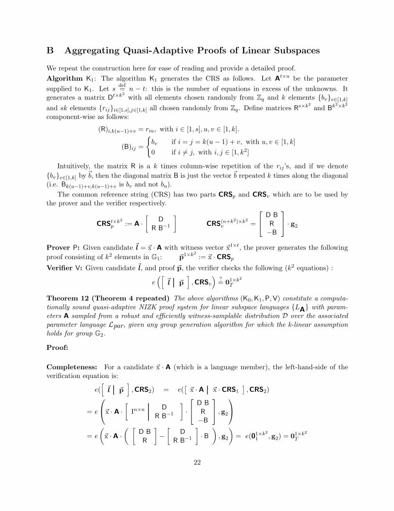
We repeat the construction here for ease of reading and provide a detailed proof.



generates a matrix Dt×k2 with all elements chosen randomly from Zq and k elements {bv}v∈[1,k]

and sk elements {rij}i∈[1,s],j∈[1,k] all chosen randomly from Zq. Define matrices Rs×k2 and B

k2×k2


(R)i,k(u−1)+v = riu, with i ∈ [1, s], u, v ∈ [1, k].

(B)ij =

{

bv if i = j = k(u− 1) + v, with u, v ∈ [1, k]

0 if i 6= j, with i, j ∈ [1, k2]

Intuitively, the matrix R is a k times column-wise repetition of the rij’s, and if we denote

{bv}v∈[1,k] by ~b, then the diagonal matrix B is just the vector ~b repeated k times along the diagonal(i.e. Bk(u−1)+v,k(u−1)+v is bv and not bu).


CRSt×k2

p := A ·

[

D

R B−1

]

CRS(n+k2)×k2v =

D B

R

−B

· g2

Prover P: Given candidate ~l = ~x · A with witness vector ~x1×t, the prover generates the following

proof consisting of k2 elements in G1: ~p1×k2 := ~x · CRSp

Verifier V: Given candidate ~l , and proof ~p, the verifier checks the following (k2 equations) :

e([

~l ~p]

,CRSv

)

?= 01×k

2

T

Theorem 12 (Theorem 4 repeated) The above algorithms (K0,K1,P,V) constitute a computa-tionally sound quasi-adaptive NIZK proof system for linear subspace languages {LA} with param-eters A sampled from a robust and efficiently witness-samplable distribution D over the associatedparameter language Lpar, given any group generation algorithm for which the k-linear assumptionholds for group G2.

Proof:

Completeness: For a candidate ~x · A (which is a language member), the left-hand-side of theverification equation is:

e([

~l ~p]

,CRS2) = e([

~x · A ~x · CRS1

]

,CRS2)

= e

~x ·A ·

[

In×nD

R B−1

]

·

D B

R

−B

,g2

= e

(

~x ·A ·

( [

D B

R

]

−

[

D

R B−1

]

· B

)

,g2

)

= e(01×k2

1 ,g2) = 01×k2

T

22

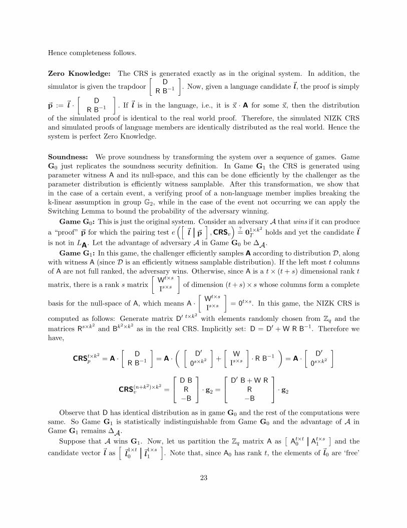
Hence completeness follows.

Zero Knowledge: The CRS is generated exactly as in the original system. In addition, the

simulator is given the trapdoor

[

D

R B−1

]

. Now, given a language candidate ~l , the proof is simply

~p := ~l ·

[

D

R B−1

]

. If ~l is in the language, i.e., it is ~x · A for some ~x, then the distribution

of the simulated proof is identical to the real world proof. Therefore, the simulated NIZK CRSand simulated proofs of language members are identically distributed as the real world. Hence thesystem is perfect Zero Knowledge.

Soundness: We prove soundness by transforming the system over a sequence of games. GameG0 just replicates the soundness security definition. In Game G1 the CRS is generated usingparameter witness A and its null-space, and this can be done efficiently by the challenger as theparameter distribution is efficiently witness samplable. After this transformation, we show thatin the case of a certain event, a verifying proof of a non-language member implies breaking thek-linear assumption in group G2, while in the case of the event not occurring we can apply theSwitching Lemma to bound the probability of the adversary winning.

Game G0: This is just the original system. Consider an adversary A that wins if it can produce

a “proof” ~p for which the pairing test e([

~l ~p]

,CRSv

)

?= 01×k

2

T holds and yet the candidate ~l

is not in LA. Let the advantage of adversary A in Game G0 be ∆A.

Game G1: In this game, the challenger efficiently samples A according to distribution D, alongwith witness A (since D is an efficiently witness samplable distribution). If the left most t columnsof A are not full ranked, the adversary wins. Otherwise, since A is a t× (t+ s) dimensional rank t

matrix, there is a rank s matrix

[

Wt×s

Is×s

]

of dimension (t+ s)× s whose columns form a complete

basis for the null-space of A, which means A ·

[

Wt×s

Is×s

]

= 0t×s. In this game, the NIZK CRS is

computed as follows: Generate matrix D′ t×k2 with elements randomly chosen from Zq and the

matrices Rs×k2 and B

k2×k2 as in the real CRS. Implicitly set: D = D′ + W R B

−1. Therefore wehave,

CRSt×k2

p = A ·

[

D

R B−1

]

= A ·

( [

D′

0s×k2

]

+

[

W

Is×s

]

· R B−1

)

= A ·

[

D′

0s×k2

]

CRS(n+k2)×k2v =

D B

R

−B

· g2 =

D′B+W R

R

−B

· g2

Observe that D has identical distribution as in game G0 and the rest of the computations weresame. So Game G1 is statistically indistinguishable from Game G0 and the advantage of A inGame G1 remains ∆A.


At×t0 A

t×s1

]

and the


~l1×t

0~l1×s

1

]


23


member vector ~l ′ can be computed as ~l ′ :=[

~l0 −~l0 ·W]

, where W = −A−10 A1. The proof of ~l′

is computed as ~p ′ := ~l0 · D′. Since A wins G1, then (~l , ~p) passes the verification test, and further

by design (~l′, ~p′) passes the verification test. Thus, we obtain: (~l

′

1 −~l1) · R = (~p′ − ~p) · B, where

~l′

1 = −~l0 ·W.

This gives us a set of equalities, for all u ∈ [1, k]:

s∑

i=1

(l ′1i − l1i) · riu = (p′k(u−1)+1 − pk(u−1)+1) · b1 = · · · = (p′k(u−1)+k − pk(u−1)+k) · bk (13)

Also note that since ~l is not in the language, there exists an i ∈ [1, s], such that ~l′

1i −~l1i 6= 0.

Game G2: Game G2 is exactly set up as Game G1, except that we restrict A to win in GameG2 only if it wins Game G1 and Event E does not occur, where E is defined as follows:


i=1

(l ′1i − l1i) · riu 6= 01 (14)

Therefore, we have: Pr[A wins G1] = Pr[A wins G1 ∧ E] +Pr[A wins G2]. We show now thatthe first term is upper bounded by adv(klin). To do that we construct a k-linear adversary B fromA and part of the Game G1 challenger, such that if A wins G1 and Event E occurs, B is able towin the k-linear challenge.

So suppose, B is given a k-linear instance (b1 · g2, ..., bk · g2, g2, b1s1 · g2, ..., bksk · g2, χ)in the group G2, where χ is either (s1 + ... + sk) · g2 or random. B then computes the matrixB · g2 by setting (B · g2)k(u−1)+v,k(u−1)+v = bv · g2 and setting all the non-diagonal elements to02. The adversary B then generates the matrices A,R and D

′ and computes A := A · g1 and theCRS’es CRSp and CRSv from these matrices and the matrix B · g2, similar to Game G1. After

that, adversary A is given A,CRSp and CRSv. Adversary A returns (~l , ~p), from which B computes

(~l′

1−~l1), identically as in the description of Game G1. Now we condition on the event that A wins

G1 and event E occurs. Then,∑s

i=1(l′1i − l1i) · riu is non-zero for some u ∈ [1, k], say for u = w.

This w can be efficiently computed by B since it has all the riu’s. Now B performs the followingtest:

e

(

s∑

i=1

(l ′1i − l1i) · riw,χ

)

?=

k∑

j=1

e(p′k(w−1)+j − pk(w−1)+j, bjsj · g2).

In the case χ is equal to (s1 + ... + sk) · g, the equality will hold by virtue of Equation 13. In thecase χ is random, the equality will not hold. Thus we have: Pr[A wins G1 ∧ E] ≤ adv(klin).

Game G3: We now prepare to employ the Switching Lemma. To do that, in Game G3,we replace R in the verification test by R

′, which we define as follows: Generate sk elements{r′ij}i∈[1,s],j∈[1,k] all chosen randomly from Zq. Now set:

(R′)i,k(u−1)+v = r′iu, with i ∈ [1, s], u, v ∈ [1, k].

Note that CRSp and CRSv remain the same as GameG2, i.e. use R, and it is only the verification

test which changes to e([

~l ~p]

,CRS′v

)

?= 01×k

2

T where CRS′v uses R

′ instead of R. We claim

24

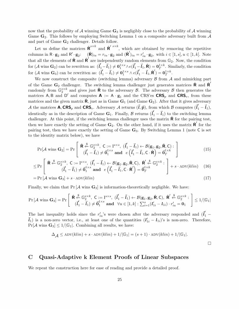
now that the probability of A winning Game G3 is negligibly close to the probability of A winningGame G2. This follows by employing Switching Lemma 1 on a composite adversary built from Aand part of Game G2 challenger. Details follow.

Let us define the matrices Rs×k

and R′ s×k

, which are obtained by removing the repetitive

columns in R · g2 and R′ · g2: (R)iu = riu · g2 and (R

′)iu = r′iu · g2, with i ∈ [1, s], u ∈ [1, k]. Note

that all the elements of R and R′are independently random elements from G2. Now, the condition

for (A wins G2) can be rewritten as: (~l′

1−~l1) 6= 01×s1 ∧e(~l

′

1−~l1, R) = 01×kT . Similarly, the condition

for (A wins G3) can be rewritten as: (~l′

1 −~l1) 6= 01×s1 ∧ e(~l

′

1 −~l1, R

′) = 01×k

T .

We now construct the composite (switching lemma) adversary B from A and mimicking part

of the Game G2 challenger. The switching lemma challenger just generates matrices R and R′

randomly from Gs×k2 and gives just R to the adversary B. The adversary B then generates the

matrices A,B and D′ and computes A := A · g1 and the CRS’es CRSp and CRSv, from these

matrices and the given matrix R, just as in Game G1 (and Game G2). After that it gives adversary

A the matrices A,CRSp and CRSv. Adversary A returns (~l , ~p), from which B computes (~l′

1 −~l1),

identically as in the description of Game G1. Finally, B returns (~l′

1 −~l1) to the switching lemma

challenger. At this point, if the switching lemma challenger uses the matrix R for the pairing test,

then we have exactly the setting of Game G2. On the other hand, if it uses the matrix R′for the

pairing test, then we have exactly the setting of Game G3. By Switching Lemma 1 (note C is setto the identity matrix below), we have

Pr[A wins G2] = Pr

R$←− G

s×k2 , C := Is×s, (~l

′

1 −~l1)← B(g1,g2, R,C) :

(~l′

1 −~l1) 6= ~0

1×s1 and e

(

~l′

1 −~l1,C · R

)

= ~01×kT

(15)

≤Pr

R$←− G

s×k2 , C := Is×s, (~l

′

1 −~l1)← B(g1,g2, R,C), R

′ $←− G

s×k2 :

(~l′

1 −~l1) 6= ~0

1×s1 and e

(

~l′

1 −~l1,C · R

′)

= ~01×kT

+ s · adv(klin) (16)

=Pr [A wins G3] + s · adv(klin) (17)

Finally, we claim that Pr [A wins G3] is information-theoretically negligible. We have:

Pr [A wins G3] = Pr

[

R$←− G

s×k2 , C := Is×s, (~l

′

1 −~l1)← B(g1,g2, R,C), R

′ $←− G

s×k2 :

(~l′

1 −~l1) 6= ~0

1×s1 and ∀u ∈ [1, k] :

∑si=1(l

′1i − l1i) · r

′iu = 01

]

≤ 1/|G1|

The last inequality holds since the r′iu’s were chosen after the adversary responded and (~l′

1 −~l1) is a non-zero vector, i.e., at least one of the quantities (l ′1i − l1i)’s is non-zero. Therefore,Pr[A wins G3] ≤ 1/|G1|. Combining all results, we have:

∆A ≤ adv(klin) + s · adv(klin) + 1/|G1| = (s+ 1) · adv(klin) + 1/|G1|.

�

C Quasi-Adaptive k Element Proofs of Linear Subspaces

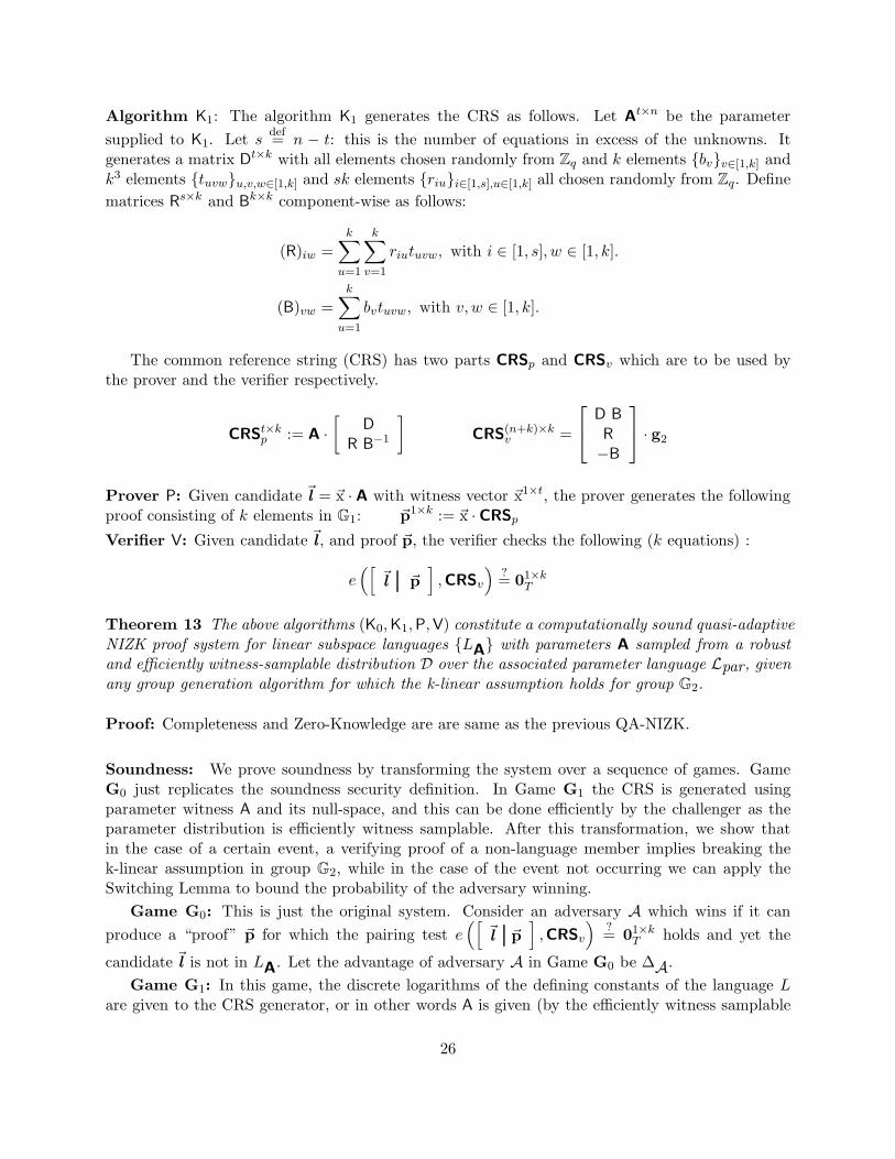
We repeat the construction here for ease of reading and provide a detailed proof.

25



generates a matrix Dt×k with all elements chosen randomly from Zq and k elements {bv}v∈[1,k] and

k3 elements {tuvw}u,v,w∈[1,k] and sk elements {riu}i∈[1,s],u∈[1,k] all chosen randomly from Zq. Define

matrices Rs×k and Bk×k component-wise as follows:

(R)iw =k∑

u=1

k∑

v=1

riutuvw, with i ∈ [1, s], w ∈ [1, k].

(B)vw =k∑

u=1

bvtuvw, with v,w ∈ [1, k].


CRSt×kp := A ·

[

D

R B−1

]

CRS(n+k)×kv =

D B

R

−B

· g2

Prover P: Given candidate ~l = ~x · A with witness vector ~x1×t, the prover generates the followingproof consisting of k elements in G1: ~p1×k := ~x · CRSp

Verifier V: Given candidate ~l , and proof ~p, the verifier checks the following (k equations) :

e([

~l ~p]

,CRSv

)

?= 01×kT

Theorem 13 The above algorithms (K0,K1,P,V) constitute a computationally sound quasi-adaptiveNIZK proof system for linear subspace languages {LA} with parameters A sampled from a robustand efficiently witness-samplable distribution D over the associated parameter language Lpar, givenany group generation algorithm for which the k-linear assumption holds for group G2.

Proof: Completeness and Zero-Knowledge are are same as the previous QA-NIZK.

Soundness: We prove soundness by transforming the system over a sequence of games. GameG0 just replicates the soundness security definition. In Game G1 the CRS is generated usingparameter witness A and its null-space, and this can be done efficiently by the challenger as theparameter distribution is efficiently witness samplable. After this transformation, we show thatin the case of a certain event, a verifying proof of a non-language member implies breaking thek-linear assumption in group G2, while in the case of the event not occurring we can apply theSwitching Lemma to bound the probability of the adversary winning.

Game G0: This is just the original system. Consider an adversary A which wins if it can

produce a “proof” ~p for which the pairing test e([

~l ~p]

,CRSv

)

?= 01×kT holds and yet the

candidate ~l is not in LA. Let the advantage of adversary A in Game G0 be ∆A.

Game G1: In this game, the discrete logarithms of the defining constants of the language Lare given to the CRS generator, or in other words A is given (by the efficiently witness samplable

26

property). Since A is a t× (t+ s) dimensional rank t matrix, there is a rank s matrix

[

Wt×s

Is×s

]

of

dimension (t + s) × s whose columns form a complete basis for the null-space of A, which means

A ·

[

Wt×s

Is×s

]

= 0t×s. In this game, the NIZK CRS is computed as follows: Generate matrix D′ t×k

with elements randomly chosen from Zq and the matrices Rs×k and B

k×k as in the real CRS.Implicitly set: D = D

′ +W R B−1. Therefore we have,

CRSt×kp = A ·

[

D

R B−1

]

= A ·

( [

D′

0s×k

]

+

[

W

Is×s

]

· R B−1

)

= A ·

[

D′

0s×k

]

CRS(n+k)×kv =

D B

R

−B

· g2 =

D′B+W R

R

−B

· g2

Observe that D has identical distribution as in game G0 and the rest of the computations weresame. So Game G1 is statistically indistinguishable from Game G0 and the advantage of A inGame G1 remains ∆A.


At×t0 A

t×s1

]

and the


~l1×t

0~l1×s

1

]



member vector ~l ′ can be computed as ~l ′ :=[

~l0 −~l0 ·W]

, where W = −A−10 A1. The proof of ~l′

is computed as ~p ′ := ~l0 · D′. Since A wins G1, then (~l , ~p) passes the verification test, and further

by design (~l′, ~p′) passes the verification test. Thus, we obtain: (~l

′

1 −~l1) · R = (~p′ − ~p) · B, where

~l′

1 = −~l0 ·W.

This gives us a set of equalities:

For all w ∈ [1, k] :

s∑

i=1

[

(l ′1i − l1i) ·

(

k∑

u=1

k∑

v=1

riutuvw

)]

−

k∑

v=1

[

(p′v − pv) ·

(

k∑

u=1

bvtuvw

)]

= 01

(18)Rearranging, we get:

For all w ∈ [1, k] :k∑

u=1

k∑

v=1

[

tuvw

(

s∑

i=1

[

(l ′1i − l1i) · riu]

− (p′v − pv) · bv

)]

= 01 (19)

Also note that since ~l is not in the language, there exists an i ∈ [1, s], such that ~l′

1i −~l1i 6= 0.

Game G2: Let us now define the following event F :

F ≡ For some u, v ∈ [1, k] :

(

s∑

i=1

[

(l ′1i − l1i) · riu]

− (p′v − pv) · bv

)

6= 01

We define that A wins in Game G2 if A wins in Game G1 and event F does not occur. Now weshow that Pr[A wins G2] is negligibly close to Pr[A wins G1]. We establish this by showing thatPr[A wins G1 ∧ F ] is negligible.

27

We now prepare to employ the Switching Lemma. To do that, Generate k3 elements{t′uvw}u,v,w∈[1,k] all chosen randomly from Zq. Now we replace T in the verification test by T

′

in a Game G1′, related to Game G1, which we define as follows:

(T)k(u−1)+v,w = tuvw, with u, v, w ∈ [1, k].

(T′)k(u−1)+v,w = t′uvw, with u, v, w ∈ [1, k].

Note that CRSp and CRSv remain the same as GameG1, i.e. use T, and it is only the verification

test which changes to e([

~l ~p]

,CRS′v

)

?= 01×k

T where CRS′v uses T′ instead of T. We claim now

that the probability of A winning Game G1′ is negligibly close to the probability of A winning

Game G1 and the event F occurring.

The claim is established by constructing a switching lemma adversary, such that winning GameG1 corresponds to one scenario and winning Game G1

′ corresponds to the other scenario. Oncethat is done, the switching lemma lets us reason that the probabilities of winning are negligiblyclose under the k-linear assumption.

We construct a switching lemma attacker B from A and part of the Game G1 challenger. Theswitching lemma challenger just generates matrices T and T

′ randomly from Gk2×k2 and gives just

T to the adversary B. The adversary B then generates the A, {riu}i∈[1,s],u∈[1,k], {bv}v∈[1,k] and D′

and computes A := A · g1 and the CRS’es CRSp and CRSv, from these matrices and the givenmatrix T, just as in Game G1. After that, adversary A is given A,CRSp and CRSv. Adversary

A returns (~l , ~p), from which B computes (~l′

1 −~l1), identically as in the description of Game G1.

Then B computes the vector ~f1×k2

with the [k(u− 1) + v]-th component equal to:

fk(u−1)+v =s∑

i=1

[

(l ′1i − l1i) · riu]

− (p′v − pv) · bv

Finally, B returns ~f to the switching lemma challenger. At this point, if the switching lemmachallenger uses the matrix T for the pairing test, then we exactly have the setting of Game G1.On the other hand, if it uses the matrix T

′ for the pairing test, then we exactly have the setting ofGame G1

′.

Pr[A wins G1 ∧ F ] = Pr

T$←− G

k2×k2 , C := Ik×k, ~f← B(g1,g2,T,C) :

~f 6= ~01×k2

1 and e(

~f,C ·T)

= ~01×kT

(20)

≤Pr

T$←− G

k2×k2 , C := Ik×k, ~f← B(g1,g2,T,C), T

′ $←− G

k2×k2 :

~f 6= ~01×k2

1 and e(

~f,C ·T′)

= ~01×kT

+ k2 · adv(klin) (21)

=Pr[

A wins G1′]

+ k2 · adv(klin) (22)

Finally, we claim that Pr [A wins G1′] is information-theoretically negligible. We have:

Pr[

A wins G1′]

= Pr

T$←− G

k2×k2 , C := Ik×k, ~f← B(g1,g2,T,C), T

′ $←− G

k2×k2 :

~f 6= ~01×k2

1 and e(

~f,C ·T′)

= ~01×kT

≤ 1/|G1|

28

The last inequality holds since the t′uvw’s were chosen after the adversary responded and~f is a non-zero vector, i.e., at least one of the quantities fi’s is non-zero. Therefore, Pr[A wins G1

′] ≤ 1/|G1|.

Game G3: Game G3 is exactly set up as Game G2, except that we restrict A to only win inGame G3 if it wins Game G1 and Event E does not occur, where E is defined as follows:


i=1

(l ′1i − l1i) · riu 6= 01 (23)

Recall that the event F defined in Game G1 does not occur in both Games G2 and G3.

Therefore, we have: Pr[A wins G2] = Pr[A wins G2 ∧ E] +Pr[A wins G3]. We show now thatthe first term is upper bounded by adv(klin). To do that we construct a k-linear adversary B fromA and part of the Game G2 challenger, such that if A wins G2 and Event E occurs, B is able towin the k-linear challenge.

So suppose, B is given a k-linear instance (b1 · g2, ..., bk · g2, g2, b1s1 · g2, ..., bksk · g2, χ)in the group G2, where χ is either (s1 + ...+ sk) ·g2 or random. B then computes the matrix B · g2

by choosing {tuvw}u,v,w∈[1,k] randomly from Zq and setting (B · g2)vw =∑k

u=1 [tuvw(bv · g2)]. Theadversary B then generates the matrices A,R and D

′ and computes A := A · g1 and the CRS’esCRSp and CRSv, from these matrices and the matrix B · g2, similar to Game G1. After that,

adversary A is given A,CRSp and CRSv. Adversary A returns (~l , ~p), from which B computes

(~l′

1−~l1), identically as in the description of Game G1. Now, since A wins G1 and event E occurs,

∑si=1(l

′1i− l1i) · riu is non-zero for some u ∈ [1, k], say for u = z, which can be computed efficiently.

Now B performs the following test:

e

(

s∑

i=1

(l ′1i − l1i) · riz,χ

)

?=

k∑

j=1

e(p′j − pj , bjsj · g2).

In the case χ is equal to (s1 + ... + sk) · g, the equality will hold by virtue of Equation 13. In thecase χ is random, the equality will not hold. Thus we have: Pr[A wins G1 ∧ E] ≤ adv(klin).

Game G4: We now prepare to employ the Switching Lemma. To do that, in Game G4, wereplace rius in the verification test by r′ius. Note that CRSp and CRSv remain the same as Game

G3, i.e. use rius, and it is only the verification test which changes to e([

~l ~p]

,CRS′v

)

?= 01×kT

where CRS′v uses r′ius instead of rius. We claim now that the probability of A winning Game G4

is negligibly close to the probability of A winning Game G3.

The claim is established by constructing a switching lemma adversary, such that winning GameG3 corresponds to one scenario and winning Game G4 corresponds to the other scenario. Oncethat is done, the switching lemma lets us reason that the probabilities of winning are negligiblyclose under the k-linear assumption.

Let us define the matrices Rs×k

and R′ s×k


(R)iu = riu · g2 and (R′)iu = r′iu · g2, with i ∈ [1, s], u ∈ [1, k].

Note that all the elements of R and R′are independently random elements from G2. Now, the

condition for (A wins G3) can be rewritten as: (~l′

1 −~l1) 6= 01×s1 ∧ e(~l

′

1 −~l1, R) = 01×kT . Similarly,

the condition for (A wins G4) can be rewritten as: (~l′

1 −~l1) 6= 01×s1 ∧ e(~l

′

1 −~l1, R

′) = 01×kT .

29

We construct a switching lemma attacker B from A and part of the Game G3 challenger. The

switching lemma challenger just generates matrices R and R′randomly from G

s×k2 and gives just

R to the adversary B. The adversary B then generates A, {tuvw}u,v,w∈[1,k] and D′ and computes

A := A · g1 and the matrix B and the CRS’es CRSp and CRSv, from these matrices and the given

matrix R, just as in Game G1. After that, adversary A is given A,CRSp and CRSv. Adversary

A returns (~l , ~p), from which B computes (~l′

1 −~l1), identically as in the description of Game G1.

Finally, B returns (~l′

1−~l1) to the switching lemma challenger. At this point, if the switching lemma

challenger uses the matrix R for the pairing test, then we exactly have the setting of Game G3.

On the other hand, if it uses the matrix R′for the pairing test, then we exactly have the setting of

Game G4.

Pr[A wins G3] = Pr

R$←− G

s×k2 , C := Is×s, (~l

′

1 −~l1)← B(g1,g2, R,C) :

(~l′

1 −~l1) 6= ~0

1×s1 and e

(

~l′

1 −~l1,C · R

)

= ~01×kT

(24)

≤Pr

R$←− G

s×k2 , C := Is×s, (~l

′

1 −~l1)← B(g1,g2, R,C), R

′ $←− G

s×k2 :

(~l′

1 −~l1) 6= ~0

1×s1 and e

(

~l′

1 −~l1,C · R

′)

= ~01×kT

+ s · adv(klin) (25)

=Pr [A wins G4] + s · adv(klin) (26)

Finally, we claim that Pr [A wins G4] is information-theoretically negligible. We have:

Pr [A wins G4] = Pr

[

R$←− G

s×k2 , C := Is×s, (~l

′

1 −~l1)← B(g1,g2, R,C), R

′ $←− G

s×k2 :

(~l′

1 −~l1) 6= ~0

1×s1 and ∀u ∈ [1, k] :

∑si=1(l

′1i − l1i) · r

′iu = 01

]

≤ 1/|G1|

The last inequality holds since the r′iu’s were chosen after the adversary responded and (~l′

1 −~l1) is a non-zero vector, i.e., at least one of the quantities (l ′1i − l1i)’s is non-zero. Therefore,Pr[A wins G4] ≤ 1/|G1|. Combining all results, we have:

∆A ≤ k2adv(klin) + adv(klin) + s · adv(klin) +O(1)/q = (k2 + s+ 1) · adv(klin) +O(1)/q.

�

D More Optimized k Element QA-NIZK Proofs

In this construction the Algorithm K1 generates the CRS as follows. It generates a matrix Dt×k

with all elements chosen randomly from Zq and k elements {bv}v∈[1,k] and k(2k − 1) elements{tuw}u∈[1,2k−1],w∈[1,k] and sk elements {riu}i∈[1,s],u∈[1,k] all chosen randomly from Zq. Define matri-

ces Rs×k and Bk×k component-wise as follows:

(R)iw =k∑

u=1

riutuw, with i ∈ [1, s], w ∈ [1, k].

(B)vw =

b1(t1w − tk+1,w) if v = 1, w ∈ [1, k]

bv(tvw − tk+v,w + tk+v−1,w) if v ∈ [2, k − 1], w ∈ [1, k]

bk(tkw + t2k−1,w) if v = k,w ∈ [1, k]

30

The construction of CRSp and CRSv remain algebraically the same. The prover and verifier alsoretain the same algebraic form. The set of equalities for this construction corresponding to the

equation (~l′

1 −~l1) · R = (~p′ − ~p) · B, is for all w ∈ [1, k]:

s∑

i=1

[

(l ′1i − l1i) ·

(

k∑

u=1

riutuw

)]

−

k−1∑

v=2

[

(p′v − pv) · bv (tvw − tk+v,w + tk+v−1,w)]

− (p′1 − p1) · b1(t1w − tk+1,w)− (p′k − pk) · bk(tkw + t2k−1,w) = 01 (27)

Rearranging, we get for all w ∈ [1, k]:

k∑

u=1

[

tuw

(

s∑

i=1

[

(l ′1i − l1i) · riu]

− (p′u − pu) · bu

)]

+

k−1∑

u=1

tu+k,w[

(p′u − pu) · bu − (p′u+1 − pu+1) · bu+1

]

= 01 (28)

Now, using the Switching Lemma and after applying information theoretic arguments, we tran-sition to a game where the adversary wins if it wins the original game and the following eventoccurs:

For all u ∈ [1, k] :s∑

i=1

(l ′1i − l1i) · riu = (p′1 − p1) · b1 = · · · = (p′k − pk) · bk (29)

After this point, the proof is analogous to the previous QA-NIZK construction. Advantageagainst soundness is now upper bounded by (2k + s) · adv(klin) +O(1)/q.

E Proof of Groth-Sahai Aggregation

Proof: [of Theorem 6] Completeness of the above system is obvious by design. In the quasi-adaptive setting the zero-knowledge simulation is required to be uniform, i.e. a single efficient TMis required to simulate the CRS given the language parameters. In the above system, the vectors ofrandomness ~ρ and ~ψ are chosen by the CRS simulator randomly as well. Then, given the languageparameters, it can generate the CRS using ~ρ and ~ψ. The zero-knowledge proof simulation is similarto the Groth-Sahai zero-knowledge proof simulation and we skip the details.

Focusing on the soundness proof, we define a sequence of games, starting with game G0 which isjust the (soundness) security definition game. The Adversary wins G0 if it can produce 〈tj1〉j∈[1,k],

commitments to ~y and ~x, as well as proofs ~πρ and ~πψ, such that 〈tj1〉j do not satisfy the aboveequations (10) and yet the verification tests (11) and (12) pass.

In game G1, the challenger (efficiently) samples ~a along with witnesses ~a (s.t. ~a = ~a · g). Thecomponent

∑

j ρj · ι2(~aj) of the CRS is now generated as

∑

j ρj · ι1(~aj). The probability of the

adversary winning G1 remains the same as winning G0.

In game G2, the challenger generates∑

j ρj · ι1(~aj) as

∑

j ι2(ρj · g) · ~aj, and

∑

j ρj · ι1(~bj) as

∑

j ι1(ρj) ·~bj (and similarly for ψ terms). Note that each of ~aj is a vector of length n, and hence the

first term is a length n vector of G3 elements, and similarly the second term is a length m vector of

31

G3 elements. Similar change occurs in the verification tests (11) and (12). Again, the probability

of the adversary winning G2 is same as winning G1.

Applying projection pT to both sides of these versions of (11) and (12), and using the commu-tativity properties mentioned above, we get that if the adversary wins G2 then

(∑

j

ρj ·~bj) · p2(~c2) + p1(~c1) · (

∑

j

ρjg ·~aj) =

∑

j

(ρj · tj1) (30)

(∑

j

ψj ·~bj) · p2(~c2) + p1(~c1) · (

∑

j

ψjg ·~aj) =

∑

j

(ψj · tj1) (31)

Thus, the probability of adversary winning G2 is at most the probability that it produces 〈tj1〉j ,~c1, ~c2 (not all zero, otherwise they are in the language), such that Equations (30) and (31) hold.

In game G3, the challenger generates the CRS as in G2 but instead of a public verification ofthe proofs and commitments, it does the following: It first generates fresh random vectors ~ρ′ and~ψ′, and performs the following bilinear pairing test (using trapdoors α and β to efficiently computep2):

∑

j

(ρ′jg)⊗ ((~bj)⊤p2(~c2) + (~aj)⊤p2(~c1)− tj1) = 0T (32)

∑

j

(ψ′jg)⊗ ((~bj)⊤p2(~c2) + (~aj)⊤p2(~c1)− tj1) = 0T (33)

The adversary wins game G3 if the k quantities 〈(~bj)⊤p2(~c2) + (~aj)⊤p2(~c1) − tj1〉 are not all zero

and the above test passes. The k quantities above being not all zero is equivalent to 〈tj1〉 not beingin the language. Note p1(~c1) has been replaced by p2(~c1). While map p2 in Groth-Sahai system isan efficient map (given trapdoors α and β), the map p1 is not efficient. However, it is the case thatp1(f) · g = p2(f) for any f in G

3. Thus, the equations (30) and (31) hold iff the tests (32) and (33)hold with ~ρ′ and ~ψ′ replaced with original ~ρ and ~ψ.

If the probability of adversary winning game G0 is ∆, then by the Switching Lemma ∆ is upperbounded by the probability of adversary winningG3 plus (k+1) ·adv(DLIN). Now, the probabilityof adversary winning game G3 is at most 1/|q|2, and that completes the proof. �

F QA-NIZK Extension with Tags

In this section we show how the system of Section 4 can be extended to include tags mirroring [JR13].The tags are elements of Zq, are included as part of the proof and are used as part of the definingequations of the language.

While our system works for any number of components in the tuple (except the first t) beingdependent on any number of tags, to simplify the presentation we will focus on only one dependentelement and only one tag. Also for simplicity, we will assume that this element is an affine functionof the tag. These languages can be characterized as

LA,~a1,~a2={⟨

~x ·[

A (~a⊤1 + tag · ~a⊤2 )]

,tag⟩

| ~x ∈ Zqt,tag ∈ Zq

}

where At×(n−1), ~a1×t1 and ~a1×t2 are parameters of the language. A distribution is still called robust

(as in Section 4) if with overwhelming probability the first t columns of A are full-ranked.

32

Algorithm K1: The CRS is generated as:

CRSt×kp,0 :=

[

A ~a⊤1]

·

[

D1

R B−1

]

CRSt×kp,1 :=

[

A ~a⊤2]

·

[

D2

R B−1

]

CRS(n+k)×kv,0 :=

D1B

R

−B

· g2 CRS(n+k)×kv,1 :=

D2B

0s×k

0k×k

· g2

where D1 and D2 are matrices of order t×k with elements randomly chosen from Zq. The matricesRs×k and B

k×k are generated just as in Section 4.

Prover: Let ~ldef= ~x ·

[

A (~a⊤1 + tag · ~a⊤2 )]

. The prover generates the following proof:

~p1×k := ~x · (CRSp,0 + tag · CRSp,1)

Verifier: Given a proof ~p for candidate ~l the verifier checks the following:

e([

~l ~p]

,CRSv,0 + tag · CRSv,1

)

?= 01×kT

The size of the proof is k elements in the group G1. The proof of completeness, soundness andzero-knowledge for this quasi-adaptive system is similar to the QA-NIZKs of Section 4 and a proofsketch follows.

Theorem 14 The above algorithms (K0,K1,P,V) constitute a computationally sound quasi-adaptiveNIZK proof system for the tag-based linear subspace languages LA,~a1,~a2

with parameters A, ~a1, ~a2sampled from a robust and efficiently witness-samplable distribution D, given any group generationalgorithm for which the k-linear assumption holds for group G2.

Proof:

Completeness: We have,[

~l ~p]

=[

~x ·A ~x · (~a⊤1 + tag · ~a⊤2 ) ~x · (A · D1 +A · tag · D2 + (~a⊤1 + tag · ~a⊤2 ) · R B−1)

]

and

CRSv,0 + tag · CRSv,1 =

(D1 + tag · D2)BR

−B

· g2

Therefore,

e([

~l ~p]

,CRSv,0 + tag · CRSv,1

)

= e

~x · A · (D1 + tag · D2)B +

~x · (~a⊤1 + tag · ~a⊤2 ) · R −

~x · (A · D1 + A · tag · D2 + (~a⊤1 + tag · ~a⊤2 ) · R B−1) · B

,g2

= 01×kT

Zero Knowledge: This is straight-forward with the simulator being given trapdoors D1,D2 andR B

−1.

33

Soundness: As in the proof of Theorem 4, we compute the CRS’s in game G1 as follows. LetA = A · g1, ~a1 = ~a1 · g1 and ~a2 = ~a2 · g1. We split the matrix A into a t× t (non-singular) matrixA1 and a t× (n− t− 1) matrix A2, so that A = [A1 | A2]. Let A1 = A1 · g1 and A2 = A2 · g1.

Further, let

[

Wt×s1

Is×s

]

be the null-space of[

A1 A2 ~a⊤1]

and let

[

Wt×s2

Is×s

]

be the null-space

of[

A1 0t×(n−t−1) ~a⊤2]

. Then the CRS’s in game G1 are:

CRSp,0 :=[

A1 A2 ~a⊤1]

·

([

D′1

0s×k

]

+

[

W1

Is×s

]

· R B−1

)

=[

A1 A2 ~a⊤1]

·

[

D′1

0s×k

]

CRSp,1 :=[

A1 0t×(s−1) ~a⊤2

]

·

([

D′2

0s×k

]

+

[

W2

Is×s

]

· R B−1

)

=[

A1 0 ~a⊤2]

·

[

D′2

0s×k

]

CRS(n+k)×kv,0 :=

D′1B+W1R

R

−B

· g2 CRS(n+k)×kv,1 :=

D′2B+W2R

0s×k

0k×k

· g2

We now claim that Un×sdef=

[

W1 + tag ·W2

Is×s

]

is the null-space of A′ t×ndef=[

A (~a⊤1 + tag ·~a⊤2 )]

.

This is because U is an n× (n− t) matrix of rank (n− t) and satisfies:

A′U =

[

A1 A2 (~a⊤1 + tag ·~a⊤2 )]

[

W1 + tag ·W2

Is×s

]

= A1(W1 + tag ·W2) +([

A2 | ~a⊤1

]

+ tag ·[

0 | ~a⊤2

])

=[

A1 A2 ~a⊤1]

·

[

W1

Is×s

]

+ tag ·[

A1 0 ~a⊤2]

·

[

W2

Is×s

]

= 0t×s

The rest of the proof is similar to the rest of the proof of soundness in Theorem 13, since A′ definesthe tag-based language. �

G Publicly Verifiable CCA2 Secure IBE

We refer the reader to [JR13] for details, and just describe the Key Generation and Encryptionsteps here. Group operations are denoted multiplicatively for consistency with the paper.

Setup: The authority uses a group generation algorithm for which the SXDH assumption holdsto generate a bilinear group (G1,G2,GT ) with g1 and g2 as generators of G1 and G2 respectively.Assume that G1 and G2 are of order q, and let e be a bilinear pairing on G1 × G2. Then it picksc at random from Zq, and sets f = gc2. It further picks ∆1, ∆2, ∆3, ∆4, ∆5, b, d, e, u, z from Zq,and publishes the following public key PK:

g1, gb1, v1 = g−∆1·b+d

1 , v2 = g−∆2·b+e1 , v3 = g−∆3·b+c

1 , v4 = g−∆4·b+z1 , and k = e(g1,g2)

−∆5·b+u.

Consider the language:

L = {〈C1, C2, C3, i,tag, h〉 | ∃s : C1 = gs1, C2 = gbs1 , C3 = vs1 · vi ·s2 · v

tag·s3 · vh·s4 }

It also publishes the QA-NIZK CRS for the language L (which uses tags i,tag and h). It alsopublishes a 1-1, or Universal One-Way Hash function (UOWHF) H. The authority retains the

34

following master secret key MSK: g2, f (= gc2), and ∆1, ∆2, ∆3, ∆4, ∆5, d, e, u, z.

Encrypt(PK, i , M): the encryption algorithm chooses s and tag at random from Zq. It thenblinds M as C0 =M · ks, and also creates

C1 = gs1, C2 = gb·s1 , C3 = vs1 · vi ·s2 · v

tag·s3 · vh·s4 ,

where h = H(C0, C1, C2,tag, i). The ciphertext is then C = 〈C0, C1, C2, C3, tag, p1,p2〉, where〈p1,p2〉 is a QA-NIZK proof that 〈C0, C1, C2, C3, i,tag, h〉 ∈ L.

With the scheme in this paper, the ciphertext needs just 1 element of proof p, instead of thetwo presented by the authors.

35

Date post:	31-Mar-2018
Category:	Documents
Upload:	phamxuyen
View:	222 times
Download:	2 times

Switching Lemma for Bilinear Tests and Constant-size … · Switching Lemma for Bilinear Tests and...

Documents