Syllabus - Clouds and atmospheric convection

First part of the course, 10 sessions, taught by Caroline Muller(the second part of the course, 5 sessions, will be taught by Nicolas Rochetin).

I Fundamental aspects of clouds

1. Definition, basic questions2. Spatial distribution (online video ”A year of weather”)3. Visualization from space, homework and online module from meted4. Cloud classification: introduction

II Dry thermodynamics

1. First law of thermodynamics (Bohren & Albrecht Chp1)2. Ideal gas law (Bohren & Albrecht Chp2)3. Mixture of gas, Dalton’s law (Bohren & Albrecht Chp2)4. Hydrostatic approximation (e.g. Wallace & Hobbes Chp3)5. Joule’s law, enthalpy (e.g. Wallace & Hobbes Chp 3)

⇒ Summary of equations in specific form (per unit mass)

III Dry convection: application to the atmosphere

1. Potential temperature θ, dry static energy, dry adiabatic lapse rate (Bohren & Albrecht Chp3)2. Stability to dry convection, Brunt Vaisala frequency (Bohren & Albrecht Chp3)3. Centrifugal convection (Emanuel Chp12, Houze Chp2)4. Symmetric instability and slantwise convection (Emanuel Chp12, Houze Chp2)

IV Entropy, second law of thermodynamics

1. Definition and link with θ (Bohren & Albrecht Chp4)2. Second law and stability (entropy maximisation) (Bohren & Albrecht Chp4)

V Moist thermodynamics

1. Evaporation and condensation: the Clausius Clapeyron equation (Bohren & Albrecht Chp5&6)2. Moist thermodynamic variables (Emanuel Chp4)

VI Moist convection: application to the atmosphere

1. Convection of unsaturated moist air: virtual potential temperature (Emanuel Chp4)2. Equivalent potential temperature θe, moist static energy, moist adiabatic lapse rate (Emanuel Chp4;

Bohren & Albrecht Chp6)3. Skew-T diagrams, online module from meted4. Conditional instability, CIN, CAPE5. Life cycle of a convective cloud in an unstable atmosphere (Houze Chp8)

VII Phenomenology of the different cloud types

1. Cloud classification (Houze Chp1)2. Processes of cloud formation for each cloud type (Houze Chp5,6&7)3. Link with the large scales

BOOKS:”Atmospheric Sciences”, Wallace & Hobbes”Cloud Dynamics”, Houze”Atmospheric Convection”, Emanuel”Atmospheric Thermodynamics”, Bohren & Albrecht”Physics of Climate”, Peixoto & Oort

1

I - Fundamental aspects of clouds

See online slides of introduction :

http://www.lmd.ens.fr/muller/TEACHING_CLOUDS/Cours1-intros.pdf

And slides on cloud types :

http://www.lmd.ens.fr/muller/TEACHING_CLOUDS/Cours3-CloudTypes.pdf

II - Dry thermodynamics

II.1 - First law of thermodynamics

See online thermodynamics notes :

http://www.lmd.ens.fr/muller/TEACHING_CLOUDS/Cours3_thermo.pdf

⇒ dU = δW + δQ (1)

An example of work (crucial in atmospheric sciences): The work by pressure forces is given by δW = −pdVwhere V is the volume of the fluid. Note that this expression requires the change of volume to be done slowlyenough (for instance by moving a piston slowly) that the pressure remains in equilibrium at the piston surface.In other words, the speed of the movement mneed to be much slower than the speed of molecules, whoseorder of magnitude is the speed of sound ≈ 300 m s−1. Such a transformation is called quasi-static (seeBohrn & Albrecht Chp1 for a more detailed discussion).

II.2 - Ideal gas law

We consider an ideal gas of volume V with N molecules. Then

PV = NkT

where k is Boltzmann’s constant (≈ 1.38× 10−23 J K−1).We rewrite in specific form, introducing the molecular mass m and the specific gas constant R = k/m:

p =Nm

V

k

mT = ρRT.

This is the ideal gas law in specific form :

p = ρRT ⇔ pα = RT , (2)

where α = 1/ρ denotes specific volume. For dry air, R ≈ 286 J K−1 kg−1.Note that due to its dependence on the molecular mass of the gas, the specific gas constant R depends

on the gas considered.

2

⇒ The pressure is related to the change of the momentum of molecules by collision. It is thus related tothe molecular kinetik energy expressed in temperature.

Remark There is another formulation of the ideal gas law, in terms of moles:

pV =N

NA(NAk)T = NR∗T

where N is the number of moles, R∗ the universal ideal gas constant (R∗ ≈ 8, 3 J mol−1 K−1).

II.3 - Mixture of gases : Dalton’s law

Dalton’s law: The pressure of a mixture of ideal gases is the sum of the partial pressures of each ideal gaswhich would occupy the same volume V : p = p1 + p2 + ..., with piV = NikT where Ni is the number ofmolecules of gas i.

The ideal gas law becomes p =∑pi =

∑NikT/V = NkT/V ⇒ pV = NkT where N =

∑Ni is the

total number of molecules in the mixture of gases. In other words, the ideal gas law is unchanged for amixture of ideal gases, with N the total number of molecules.

Remark: One implication of Dalton’s law is that for a volume V at a given temperature T and pressurep, any ideal gas or mixture of ideal gases contains the same number of molecules N = pV/(kT ). Notably, ifwe compare a volume V at T, p of dry air the same volume of moist air (the latter containing water vapormolecules in addition to dry air molecules), the moist air is lighter than dry air. This is because the molecularmass of H2O is smaller than either O2 or N2. The number of molecules being the same by Dalton’s law,some of the dry air molecules have been replaced by water vapor molecules, which are lighter. The fact thatair containing water vapor is lighter than dry air is called the virtual effect.

Specific form (per unit mass): We introduce the density of gas i with molecular massmi andNi molecules:ρi = Nimi/V . The total density is ρ =

∑i ρi, the total number of molecules is N =

∑iNi. Then Dalton’s

law can be written

p =

∑iNiV

kT =

(∑j Njmj

V

)k∑

k Nkmk∑iNi

T

Thus for a mixture of gases:

⇒ p =∑j

ρjk

< m >T ⇒ p = ρRT , (3)

where p =∑i pi, ρ =

∑i ρi, R = k/< m >, and < m >=

∑Nimi/N is the mean molecular mass.

II.4 - Hydrostatic

We consider a continuous gas with density ρ(z) and pressure p(z). We suppose a layer of air in equilibriumbetween heights z and z+dz, layer with horizontal area A. The forces on this layer of air are gravity −ρgdzA,and pressure at the top interface −p(z+dz)A and at the bottom interface p(z)A. Thus equilibrium of forcesimplies

−ρgdzA− p(z + dz)A+ p(z)A = 0⇒ p(z + dz)− p(z)dz

= −ρg.

Taking the limit dz → 0,

∂p

∂z= −ρg . (4)

3

II.5 - Joule’s law, enthalpy

Note that internal energy is a state variable, hence a function of two variables U = U(T, V ) = U(T, p).Joule’s law for an ideal gas states that

∂U

∂V|T=cstt = 0.

Thus dU = CvdT for an ideal gas, where Cv is the heat capacity at constant volume.

(1) At constant volume, adding or removing heat to/from an ideal gas yields a change of internal energy:Indeed from the first law,

dU

dt= Cv

dT

dt= Q+ W = Q− pdV

dt

Thus at constant volume

Q =dU

dt= Cv

dT

dt

The larger Cv, the smaller the temperature response to heat added or removed.

(2) At constant pressure, adding or removing heat to/from an ideal gas yields a change of enthalphy

H = U + pV = CpT :

Indeed from the first law,

dU

dt= Q+ W = Q− pdV

dt⇒ dU

dt+d(pV )

dt=dH

dt= Q+ V

dp

dt

Note that H = U+pV = CvT +NkT = CpT where Cp = Cv+Nk is that heat capacity at constant pressure.Thus at constant pressure

Q =dH

dt= Cp

dT

dt.

⇒ Summary of equations in specific form:In atmospheric science, we express thermodynamic quantities in specific form, i.e. per unit mass M =

N ×m (as usual, N is the number of molecules and m the molecular mass).Recall also that α denotes specific volume 1/ρ and we introduce

cv =CvM, cp =

CpM, u =

U

M, h =

H

Mand δq =

δQ

M.

Then the equations become:

p = ρRT ⇔ pα = RT : Ideal gas law, (5)

∂p

∂z= −ρg ⇔ g dz = −αdp : Hydrostatic approximation, (6)

δq = du+ p dα = dh− αdp, with h = u+ pα : First law of thermodynamics, (7)

du = cvdT and dh = cpdT , with cp = cv +R : Joule’s law, (8)

Note that those specific variables are NOT extensive variables. One needs to multiply by the mass torecover extensive variables. In other words for a mixture of gases with masses M1 and M2, and specificinternal energies u1 and u2, the total internal energy of the mixture is U = M1u1 + M2u2 and the totalspecific internal energy is u = (M1u1 +M2u2)/(M1 +M2).

4

III - Dry convection: application to the atmosphere

Cloud formation is closely related to the convective movement of air. Thus a key question is what makesthe air move. Note that although temperature decreases with height, the cold air aloft is not heavier andthus does not “fall” to the ground, as its density is not only a function of temperature, but also of pressureρ(T, p). The three are related through the ideal gas law

p = ρRT

where R denotes the specific constant of the gas.To determine the stability of air, we thus need to account for changes in T and p with height. We use

the so-called “parcel method” to assess whether a parcel of air is unstable to upward motion. We consider ahypothetical parcel of air near the surface displaced vertically adiabatically, and ask the following question:if this parcel of air is displaced upwards, will it return to its original position, or will it keep rising? If thedisplaced parcel has lower density than the environment, it is lighter and will keep rising: the atmosphere isunstable to dry convection. If instead its density is larger, it is heavier and will accelerate back down: theatmosphere is stable to dry convection. The displacement is supposed to be slow enough that the pressureof the parcel is always in equilibrium with the pressure of the environment (“quasi-static” displacement; see§ II.1).

III.1 Potential temperature θ, dry static energy, dry adiabatic lapserate

- Conservation of potential temperature

We now show that during the quasi-static adiabatic parcel displacement, there is an invariant called potentialtemperature

θdef= T (p/p0)−R/cp , (9)

where T denotes temperature, p pressure, p0 a reference pressure (typically 1000 hPa), and cp heat capacityat constant pressure (cp ≈ 1006 J kg−1 K−1 for dry air). Then we will use this invariant to determine thecondition under which the atmosphere is unstable to dry convection.

Applying the first law of thermodynamics to an infinitesimal displacement, the change in internal energycvdT is equal to the heat added, which is zero in this adiabatic displacement, plus the work done on theparcel, in that case due to pressure forces δW = −pd(1/ρ):

cvdT = −pd(

1

ρ

). (10)

Using the ideal gas law p = ρRT and recalling that cv +R = cp, we obtain

cvdT = −p d(RT

p

)= −RdT +RT

dp

p⇔ cpdT −RT

dp

p= 0 (11)

implyingdT

T− R

cp

dp

p= d ln(Tp−R/cp) = 0. (12)

This shows that Tp−R/cp is constant, hence θ = T (p/p0)−R/cp is conserved during the displacement.

5

- Conservation of dry static energy and dry adiabatic lapse rate

Before assessing the stability of the parcel, we note that in the special case of a hydrostatic atmosphere, i.e.assuming dp = −ρgdz, the variable

hdrydef= cpT + gz (13)

is conserved. It is called the dry static energy. Indeed if we make this hydrostatic approximation, equation(12) becomes

cpdT +RTρgdz

p= d(cpT + gz) = dhdry = 0, (14)

where we have again used the ideal gas law p = ρRT . Thus the dry static energy cpT + gz is conserved inan adiabatic quasi-static displacement under the hydrostatic approximation.

Furthermore in that case, it is readily seen from equation (14) that the dry adiabatic lapse rate Γd,defined as the decrease of temperature with height, is given by

Γddef= −dT

dz=

g

cp≈ 10◦ K / km. (15)

⇒ A dry adiabat loses 1 degree every 100m.

III.2 Stability to dry convection, Brunt-Vaisala frequency

- How can we assess the stability of dry air?

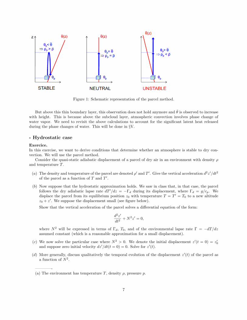
We now return to our original question, namely is the displaced parcel lighter or heavier than its environment.Recall that the pressure of the parcel is equal to that of the environment, so that during the displacementits pressure changes following the environmental pressure, while its temperature changes such that thepotential temperature is conserved. To fix ideas, let’s raise a parcel upwards (a similar argument can bemade for downward displacements). Figure 1 schematically describes the three possible cases, depending onthe environmental potential temperature profile θ, shown in red as a function of height.

The displaced parcel starts with the near-surface environmental value θp = θ, and conserves its potentialtemperature θp during its adiabatic ascent (blue). Once displaced, comparing θp with θ at the displacedpressure level determines whether the parcel is heavier or lighter than the environment. If θ increases withheight (left panel), the displaced parcel has colder potential temperature than the environment θp < θ, andthus is heavier and accelerates back down: the atmosphere is stable to dry convection. On the other hand,if θ decreases with height (right panel), the displaced parcel has warmer potential temperature than theenvironment θp > θ, and thus is lighter and keeps rising: the atmosphere is unstable to dry convection. If θis constant with height (middle panel), the displaced parcel is neither accelerated downwards nor upwards:the atmosphere is neutral to dry convection.

In the stable case, the displaced parcel will accelerate back towards and passed its original equilibriumaltitude. It will then be lighter than the environment and accelerate back up towards its equilibrium altitude.Thus the displaced parcel oscillates around its equilibrium height. The frequency of oscillation is known asthe buoyancy frequency, or Brunt Vaisala frequency, which we will show is given by:

N =

√g

θ

∂θ

∂z.

In the unstable case, convection is very efficient at removing the instability. Indeed, in the planetarysubcloud layer (first kilometer of the atmosphere or so), the convective adjustment time scale is very fast(minutes for dry convection) compared to destabilizing factors (surface warming, atmospheric radiativecooling...). Thus the observed state is very close to convective neutrality θ =constant, see for instance thereview [Stevens “Atmospheric Moist Convection” 2005] and references therein.

6

Figure 1: Schematic representation of the parcel method.

But above this thin boundary layer, this observation does not hold anymore and θ is observed to increasewith height. This is because above the subcloud layer, atmospheric convection involves phase change ofwater vapor. We need to revisit the above calculations to account for the significant latent heat releasedduring the phase changes of water. This will be done in §V.

- Hydrostatic case

Exercice.In this exercise, we want to derive conditions that determine whether an atmosphere is stable to dry con-vection. We will use the parcel method.

Consider the quasi-static adiabatic displacement of a parcel of dry air in an environment with density ρand temperature T .

(a) The density and temperature of the parcel are denoted ρ′ and T ′. Give the vertical acceleration d2z′/dt2

of the parcel as a function of T and T ′.

(b) Now suppose that the hydrostatic approximation holds. We saw in class that, in that case, the parcelfollows the dry adiabatic lapse rate dT ′/dz = −Γd during its displacement, where Γd = g/cp. Wedisplace the parcel from its equilibrium position z0 with temperature T = T ′ = T0 to a new altitudez0 + z′. We suppose the displacement small (see figure below).

Show that the vertical acceleration of the parcel solves a differential equation of the form:

d2z′

dt2+N2z′ = 0,

where N2 will be expressed in terms of Γd, T0, and of the environmental lapse rate Γ = −dT/dzassumed constant (which is a reasonable approximation for a small displacement).

(c) We now solve the particular case where N2 > 0. We denote the initial displacement z′(t = 0) = z′0and suppose zero initial velocity dz′/dt(t = 0) = 0. Solve for z′(t).

(d) More generally, discuss qualitatively the temporal evolution of the displacement z′(t) of the parcel asa function of N2.

————-(a) The environment has temperature T , density ρ, pressure p.

7

z0

z0 + z’

T = Tparcel = T0

parcel displaced

Figure 2: Schematic of parcel method

The parcel has temperature T ′ and density ρ′. By definition, a quasi-static displacement is such that theparcel pressure is in equilibrium with the environment p = p′.

By Archimedes’ principle, the acceleration of the parcel is

ρ′d2z′

dt2= (ρ− ρ′)g,

with p = ρRT = ρ′RT ′ (ideal gas law).Thus

d2z′

dt2=ρ− ρ′

ρ′g =

p/RT − p/RT ′

p/RT ′g =

T ′ − TT

g

(b) We suppose hydrostatic balance and displace the parcel from z0 (T=T’=T0) to z0 + z′ (small dis-placement). The displaced parcel has vertical acceleration from (a) given by

d2z′

dt2=T ′(z0 + z′)− T (z0 + z′)

T (z0 + z′)g.

Now the parcel follows a dry adiabatic lapse rate Γd = g/cp during its displacement, thus

T ′(z0 + z′) = T ′(z0)− Γdz′ = T0 − Γdz

′.

Similarly, if we denote Γ = −dT/dz the environmental lapse rate, then the temperature of the environmentat z0 + z′ is

T (z0 + z′) = T (z0)− Γz′ = T0 − Γz′.

Thusd2z′

dt2=

(T0 − Γdz′)− (T0 − Γz′)

T0 − Γz′g =

Γ− ΓdT0 − Γz′

gz′ ≈ Γ− ΓdT0

gz′,

where in the last approximation, we have used the fact that the displacement is small, thus Γz′ � T0 isneglected.

⇒ d2z′

dt2 +N2z′ = 0, where N2 = g Γd−ΓT0

(c) In the particular case where N2 > 0, the solutions of this eqquation are given by z′(t) = A cos(Nt) +B sin(Nt), where A and B are constants. From initial conditions z′(t = 0) = z′0 ⇒ A = z′0 and dz′/dt =−AN sin(Nt) +BN cos(Nt)⇒ B = 0. Thus z′(t) = z′0 cos(Nt). The displacement oscillates with frequencyN and amplitude z′0.

(d) More generally, the temporal evolution of z′(t) depends on the sign of N2. In other words, thestability of a temperature profile T (z) to dry convection under the hydrostatic approximation depends on

8

the sign of N2 = g Γd−ΓT0

. Γ is the environmental lapse rate (= −dT/dz) and Γd is the dry adiabatic lapserate g/cp. N is called the Brunt-Vaisala frequency.

If N2 > 0, i.e. if Γd > Γ, then N is real and z′(t) ∝ cos(Nt), sin(Nt). The parcel oscillates with frequencyN , Brunt-Vaisala frequency (sometimes also called buoyancy frequency). The atmosphere is stable to dryconvection.

If N2 < 0, i.e. if Γd < Γ, then N is imaginary and z′(t) ∝ exp(|N |t). There is an exponentially growingsolution z′(t) ∝ exp(|N |t) and the atmosphere is unstable to dry convection.

- General case

We now consider the general case, i.e. we do not assume hydrostasy anymore. We will show that we canstill derive a stability criterion. We know from the first law of thermodynamics that the parcel conservesits potential temperature θparcel = Tparcel(pparcel/p0)−R/cp during the displacement. Thus θparcel(z0) =θparcel(z

′ + z0). We denote the environmental potential temperature θ and density ρ.From Archimedes principle, the vertical acceleration of the parcel displaced from its equilibrium position

z0 to the new position z′ + z0 is

d2z′

dt2= g

ρ− ρparcelρparcel

= gp/T − p/Tparcel

p/Tparcel= g

Tparcel − TT

= gθparcel − θ

θ

where we have used the ideal gas law and the fact that the parcel pressure is equal to that of the environment,and where all the quantities are evaluated at (z0 + z′).

Now θparcel(z0 + z′) = θparcel(z0) = θ(z0), and θ(z0 + z′) ≈ θ(z0) + (∂θ/∂z)z′. Thus

d2z′

dt2= g

θ(z0)− (θ(z0) + (∂θ/∂z)z′)

θ(z0) + (∂θ/∂z)z′≈ g−(∂θ/∂z)z′

θ(z0),

where in the denominator we have neglected the z′ contribution since we are assuming a small displacement,thus this term is small.

Therefore

d2z′

dt2+g

θ

∂θ

∂zz′ =

d2z′

dt2+N2z′ = 0 ,

with

N2 =g

θ

∂θ

∂z.

Similar to the previous, hydrostatic case, the atmosphere is stable if N2 > 0 i.e. θ increases with z.Conversely, the atmosphere is unstable to dry convection if N2 < 0 i.e. θ decreases with z.

- Link between the 2

Note that we can recover the hydrostatic case from

N2 =g

θ

∂θ

∂z:

Indeed, assuming hydrostasy,

1

θ

∂θ

∂z=

1

T

∂T

∂z− R

cpp

∂p

∂z=

1

T

(∂T

∂z− RT

cpp(−ρg)

)=

1

T

(∂T

∂z+

g

cp

)=

1

T(Γd − Γ)

where we have used the ideal gas law p = ρRT . Multiplyig by g, we indeed recover the hydrostatic Brunt-Vaisala frequency.

9

- Remark

As we saw last time, the typical time scale for dry convection in the atmosphere τN = 2π/N is of the orderof 10 minutes.

To give some orders of magnitude, if for example we consider wind blowing on mountains with typicalhorizontal spacing of 10 km, a temperature around 20◦C, and a lapse rate of 5◦ km−1, what value of windspeed yields a frequency that matches the frequency of gravity waves ?⇒ With wind speed U over topography with length scale L, the time scale between two mountains is

τtopog = L/U . The stratification time scale is τN = 2π/N , withN =√g(Γd − Γ)/T ≈

√10 ∗ (10− 5) ∗ 10−3/293

s−1 ≈ 1.3 ∗ 10−2 s−1. Thus τN = 2π/N ≈ 480 s ≈ 8 min.Both times scales will resonate when

L

U=

2π

N⇒ U =

L

2πN =

L

τN≈ 104

480m s−1 ≈ 20 m s−1.

III.3 Centrifugal convection

We now investigate the stability of a rotating fluid to horizontal displacements. As we will discuss inmore details later, the instability to vertical displacements discussed in the previous section is relevant to thetropics where the Coriolis parameter is small. But in midlatitudes where the planetary rotation is important,slantwise convection (with a displacement having both vertical and horizontal components) is relevant aswell.

- Centrifugal convection: case of a rotating fluid in cylinder

We first focus on the simple case of a fluid in rotation around the vertical axis z and investigate the stabilityto horizontal displacements. We will apply the parcel method to a ring of fluid (in dark blue figure 3).

The Navier-Stokes equations in cylindrical coordinates, neglecting viscous effects, assuming no variationalong the angle θ : ∂/∂θ = 0, and assuming constant density α = 1/ρ =constant, yield:

du

dt= −α∂p

∂r+v2

r= −α∂p

∂r+M2

r3(16)

dM

dt= −α∂p

∂θ= 0, where M = rv. (17)

From the second equation, we see that for an inviscid, symmetric motion (∂/∂θ = 0 i.e. symmetry aroundaxis of rotation), M is conserved.

We assume that the fluid is in equilibrium :

α∂p

∂r=M2

r3.

In other words, there is an equilibrium between pressure forces and centrifugal forces. We then considerthe fluid ring of figure 3 in equilibrium with the environment at r0, and displace it horizontally from r0 tor0 + r′. As before, we use the parcel method and thus suppose that the displacement does not impact theenvironmental pressure field, and that the parcel pressure is equal to that of the environment pparcel = p.

Then the equations of motion for the parcel at r = r0 + r′ are:

duparceldt

=d2r′

dt2= −α∂pparcel

∂r(r) +

M2parcel(r)

r3.

But α∂pparcel/∂r = α∂p/∂r = M2(r)/r3 and M is conserved thus Mparcel(r) = Mparcel(r0) = M(r0). Thusthe equations of motion for the parcel at r = r0 + r′ become:

d2r′

dt2= −M

2(r)

r3+M2(r0)

r3=M2(r0)−M2(r)

r3=

(M(r0)−M(r))(M(r0) +M(r))

r3≈ (M(r0)−M(r))

2M(r0)

r30

,

10

Figure 3: The ring of fluid in dark blue is displaced horizontally from r0 to r0 + r′.

where we have used the fact that the displacement is small r′ � r0. We further develop the first term onthe right hand side:

M(r0)−M(r) = M(r0)−M(r0 + r′) ≈ −dMdr

r′.

Thus

d2r′

dt2+

2M(r0)

r30

dM

drr′ = 0 .

As in the previous section for vertical displacemet z′, we see that if dM/dr > 0, the fluid is stable tohorizontal displacements. If dM/dr < 0 on the other hand, the fluid is unstable to horizontal displacements.

Note that physically, this comes from the fact that the displaced fluid conserves its angular momentumMparcel. If dM/dr < 0, the new conditions that the displaced parcel encounters correspond to a lowerenvironmental M and thus by equilibrium to a lower pressure force. Thus its centrifugal force wins and thedisplaced parcel keeps advancing.

- Centrifugal convection: atmospheric case

This is the case relevant to oscillations in a fluid in geostrophic equilibrium (equilibrium between pressureforce and Coriolis force). We consider the displacement of a tube of fluid parallel to the x-axis (figure 4) ina fluid in geostrophic equilibrium. We suppose invariance along the y-axis ∂/∂y = 0, and Coriolis parameterf =constant. We also suppose constant density thus α =constant.

The equations of motion for the displaced fluid are

du

dt− fv = −α∂p

∂x= −fvg (18)

dv

dt+ fu = −α∂p

∂y= 0⇒ v + fx = constant = M, (19)

where we have used the geostrophic velocity vg in equilibrium with the pressure field, and we have denotesM the conserved quantity M = v + fx absolute momentum.

We apply the parcel method to the tube of fluid that we displace. As usual, we suppose that the movementdoes not perturb the pressure field. The equations of motion of the parcel thus yield at x = x0 + x′:

11

Figure 4: The tube of fluid in blue is displaced horizontally from x0 to x0 + x′. vg denotes the geostrophicwind.

du

dt− fv = −fvg ⇒

du

dt=d2x′

dt2= f(v − vg) = f [(v + fx)− (vg + fx)] = f(Mparcel(x0 + x′)−Mg(x0 + x′)).

Thus

d2x′

dt2= f(Mg(x0)−Mg(x0 + x′)) ≈ −f dMg

dxx′ ⇒ d2x′

dt2+ f

dMg

dxx′ = 0

By analogy with earlier sections, we see that if dMg/dx < 0, the fluid is unstable to horizontal displace-ments. Conversely if dMg/dx > 0, the fluid is stable. This instability is sometimes called inertial instability(in the stable case, the oscillations are called inertial oscillations).

III.4 Symmetric instability and slantwise convection

READING ASSIGNMENT: See Emanuel Chapter 12.

Overview: We suppose the reference state in hydrostatic and geostrophic balance. Then

Dw

Dt= B ≈ gT − T

T(20)

Du

Dt= f(M −M), (21)

where overbars denote the reference state temperature and absolute momentum. The atmosphere can be sta-ble to horizontal and vertical displacements separately, but unstable to slantwise convection. This instabilityis known as symmetric instability. It occurs when

∂θ

∂z|M < 0 or

∂M

∂x|θ < 0

12

IV - Entropy, Second law of thermodynamics and implications forthe atmosphere

IV.1 - Definition and link with θ

- Definition

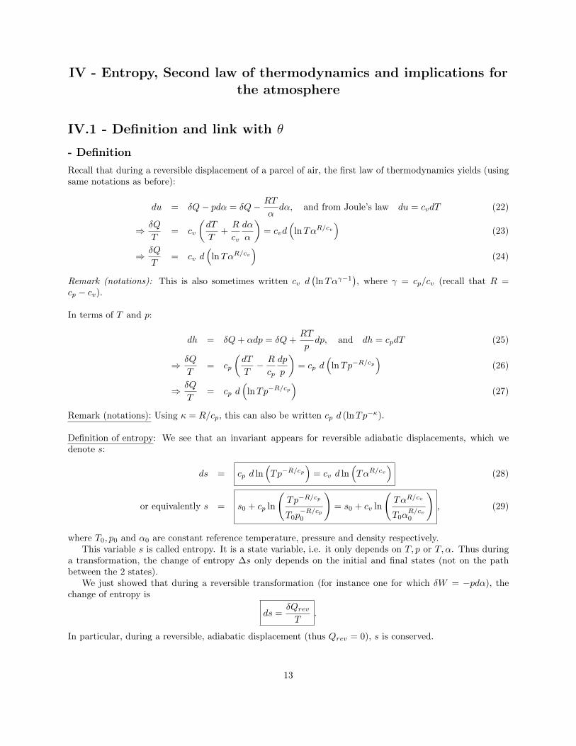
Recall that during a reversible displacement of a parcel of air, the first law of thermodynamics yields (usingsame notations as before):

du = δQ− pdα = δQ− RT

αdα, and from Joule’s law du = cvdT (22)

⇒ δQ

T= cv

(dT

T+R

cv

dα

α

)= cvd

(lnTαR/cv

)(23)

⇒ δQ

T= cv d

(lnTαR/cv

)(24)

Remark (notations): This is also sometimes written cv d(lnTαγ−1

), where γ = cp/cv (recall that R =

cp − cv).

In terms of T and p:

dh = δQ+ αdp = δQ+RT

pdp, and dh = cpdT (25)

⇒ δQ

T= cp

(dT

T− R

cp

dp

p

)= cp d

(lnTp−R/cp

)(26)

⇒ δQ

T= cp d

(lnTp−R/cp

)(27)

Remark (notations): Using κ = R/cp, this can also be written cp d (lnTp−κ).

Definition of entropy: We see that an invariant appears for reversible adiabatic displacements, which wedenote s:

ds = cp d ln(Tp−R/cp

)= cv d ln

(TαR/cv

)(28)

or equivalently s = s0 + cp ln

(Tp−R/cp

T0p−R/cp0

)= s0 + cv ln

(TαR/cv

T0αR/cv0

), (29)

where T0, p0 and α0 are constant reference temperature, pressure and density respectively.This variable s is called entropy. It is a state variable, i.e. it only depends on T, p or T, α. Thus during

a transformation, the change of entropy ∆s only depends on the initial and final states (not on the pathbetween the 2 states).

We just showed that during a reversible transformation (for instance one for which δW = −pdα), thechange of entropy is

ds =δQrevT

.

In particular, during a reversible, adiabatic displacement (thus Qrev = 0), s is conserved.

13

- Atmospheric case: link with θ

We see that

ds = cpdθ

θ

thus entropy and potential temperature are closely related. This can also be written

s = cp ln θ (up to constants).

Adiabats (trajectories with constant θ) are also sometimes called isentropes (s constant).

IV.2 - Consequences, entropy maximisation

The second law of thermodynamis states that for an isolated system, the change of entropy during a trans-formation is either 0 if this transformation is reversible, or is strictly positive if this transformation isirreversible.

This law gives us a stability criterion for an isolated system. Indeed, such a system with entropy smaximum will thus be stable, as it will not spontaneously change state (else its entropy would have todecrease which would contradict the second law).

For more on this, and the atmospheric implications of entropy maximisation, please read chapter 4 ofBohren and Albrecht (reference on the course syllabus), notably section 4.4:READING ASSIGNEMENT: Bohren Albrecht section 4.4.

Remark: For reference, we note the total entropy (not per unit mass)

dS = Cvd(lnTV (Cp−Cv)/Cv ) = Cpd(lnTp−(Cp−Cv)/Cp).

U and S are extensive, i.e. for a system composed of 2 subsystems of internal energies U1, U2 and entropiesS1, S2, the total internal energy and entropy are U = U1 + U2, S = S1 + S2. This is not true of the specificenergy and entropy.

Example 1: Instantaneous adiabatic expansion:If a gaz in a volume V1 is instantaneously expanded to a volume V2, then the work done by pressure forcesis W = 0. If the transformation is adiabatic, we thus have ∆U = W +Q = 0⇒ ∆T = 0.Then the entropy change is ∆S = Cv ln(V2/V1)(Cp−Cv)/Cv = Nk ln(V2/V1). The second law implies∆S ≥ 0⇒ V2 > V1. The gaz spontaneously occupies a larger volume.

Example 2: Reversible adiabatic expansion:In that case, the gaz is brought from a container of volume V1 to volume V2 by slowly moving a wall of thecontainer. The work of pressure forces is δW = −pdV ⇒ ds = δQ/T = 0. The entropy is constant in thisreversible adiabatic transformation.

Example 3: Entropic derivation of the dry adiabatic lapse rate:Let’s compute the dry adiabatic lapse rate Γd with the parcel method. The parcel displacement is supposedadiabatic and reversible, thus isentropic. We have

ds = cpd lnT −Rd ln p⇒ ds

dz= 0⇒ cp

T

dT

dz− R

p

dp

dz= 0.

If we further make the hydrostatic approximation, dp/dz = −ρg, and use the ideal gaz law p = ρRT , weobtain

−dTdz

= Γd =g

cp.

14

We thus recover the dry adiabatic lapse rate computed earlier.

Example 4: Application of entropy maximisation : θ = constant.The second law of thermodynamics provides a criterion for stability of an isolated system. Indeed, anisolated system with maximum entropy is stable, i.e. will not change state spontaneously nor under a smallperturbation.One implication is that the potential temperature θ is constant with height in the atmospheric boundarylayer (from the surface to cloud base, i.e. below the level of condensation of water vapor and concomitantlatent heat release).For more on this, the interested reader is referred to the book by Bohren and Albrecht page 164. We willnot cover this in detail, but the main steps are :- Consider an atmospheric layer between two isobars, of pressure p1 at height z1 and pressure p2 at heightz2. The atmosphere is supposed in hydrostatic equilibrium.- First note that its mass M is constant. Indeed M =

∫ z2z1ρdz =

∫ p1p2

dpg = 1

g (p1 − p2).

- Second note that the conservation of energy (dry static energy = enthalpy + potential energy) yields∫(cpT + gz)ρdz = constant.

- Finally note that the entropy of the layer is S =∫ρcp ln θdz =

cpg

∫ p1p2

ln θdp, and investigate the profiles of

T and p which maximize S (the optimum is θ(z) = constant).

V - Moist thermodynamics

V.1 - When does water vapor condense into liquid water? The Clausius-Clapeyronequation

What is the effect of moisture on convection? Beyond the virtual effect briefly introduced earlier, i.e. watervapor making air lighter, an important impact of moisture on convection is the condensation and concomitantlatent heat released (we will focus on vapor - liquid phase transition, though all the results below can beextended to the ice phase).

When does water vapor condense into liquid water? The water vapor contained in air will condensewhen its partial pressure ev exceeds a certain value, called the saturation partial pressure ev,s. The latter isgoverned by the Clausius-Clapeyron equation, which can be derived using the thermodynamic equilibriumbetween liquid water and water vapor:

dev,sdT

=Lvev,sRvT 2

, (30)

where ev,s is the saturation vapor pressure, T the absolute temperature, Lv the latent heat of vaporizationof water vapor and Rv the water vapor gas constant. There is net condensation when ev > ev,s(T ).

This law predicts that the saturation water vapor pressure strongly increases with temperature. Aphysical interpretation of this increase can be obtained by considering liquid water with a flat interface,above which water vapor is found with partial pressure ev. Saturation corresponds to an equilibrium betweenevaporation from the liquid water below and condensation of the water vapor above.

• ev < ev,s means that there is more evaporation than condensation,

• ev > ev,s means that there is more condensation than evaporation,

• ev = ev,s means there is as much condensation as there is evaporation.

15

Molecularly, ev,s increases with temperature because the evaporation from the liquid phase increases withtemperature, i.e. with the mean square velocity of the molecules. Thus the amount of water vapor requiredto equilibrate the evaporation is larger at larger temperatures.

We note here in passing that this is often phrased “warm air can hold more water vapor than coldair”. This is a useful shortcut to remember that the maximum amount of water vapor ev,s attainable by avolume of air before it starts to condense, is an increasing function of temperature. But it gives the wrongimpression that air is a “sponge” with holes in it, with the number of holes increasing with temperature.The saturation and condensation have nothing to do with “holes” in air, it simply has to do with equilibriumbetween evaporation and condensation. For a more in-depth discussion of the “sponge theory”, see the bookby Bohren and Albrecht (reference on the course website).

The relative humidity measures the distance to saturation, and is defined as

RH =evev,s

. (31)

It is typically expressed in percent (100% relative humidity corresponds to saturated air).

Remark 1: We just saw that ev,s(T ) only depends on temperature, following the Clausius-Clapeyron equation(30). As noted above, Lv is the latent heat of vaporization. It is the heat that the outside must provide totransform a unit mass of liquid into vapor. Or equivalently, it is the latent heat released per unit mass ofcondensation of vapor into liquid. It is given by Lv = hv − hl, difference of the specific enthalpy of watervapor and that of liquid water.

What happens during a phase change then? Let’s consider the liquid to vapor change, with liquid massMl and vapor mass Mv. The phase change occurs at constant pressure p, thus the heat Q = ∆H, whereH = Mvhv + Mlhl is the total enthalpy. Here hv and hl denote the specific enthalpies of vapor and liquidrespectively. The enthalpy change during the phase change is only due to molecular rearrangements. For amass M transformed, ∆H = Qwater = M(hv − hl) = MLv, where Lv is the heat to be added per unit massof liquid water to make it evaporate. Note that the surrounding air provides heat to the water, and thuscools Qair = −MLv .

Similary, during condensation, the latent heat released is the enthalpy difference MLv = Qair.

Remark 2: Consequence of Clausius-ClapeyronWe will see that Lv(T ) depends on T , but if we assume that it is constant (a reasonable approximation forreasonable ranges of temperatures), then the Clausius-Clapeyron equation (30) can be solved, yielding

ev,s(T ) = ev,s(T0) expLvRv

( 1T0− 1T )

In the case of a warming T = T0 + δT , with δT � T0 (as is the case for instance of a warming of a fewdegrees from a reference temperature T0 ∼ 300K), then

1

T=

1

T0(1 + δT/T0)≈ 1

T0

(1− δT

T0

)and

ev,s(T ) = ev,s(T0) expLvδT

RvT20

In other words, the water vapor amount (as measured by the partial pressure) increases quasi-exponentiallywith warming!

This has implications for the response of the hydrological cycle to climate change. Notably, we expect anintensification of precipitation extremes following Clausius-Clapeyron, at a rate of about 7-8 % K−1. Themean precipitation on the other hand is expected to increase at a slower rate, due to energy constraints (seefor instance the seminal paper Held & Soden 2006).

16

Remark 3: Similarly, the latent heat of sublimation is given by Ls = hv − hi (ice evaporates), and the latentheat of fusion is given by Lf = hl − hi (ice melts). Note that Lf + Lv = Ls, i.e. the enthalpic cost (totalheat needed) to transform ice into vapor is the same as the cost of this transformation going through theliquid phase.

Remark 4: Actually, Lv(T ) depends on temperature. Indeed,

∂Lv∂T

=∂hv∂T− ∂hl∂T

= cp,v − cp,l.

(Note that Lv is the enthalpy difference between the vapor and liquid phase of water at same saturationpressure ev,s which depends only on T , so Lv is only function of T : ∂Lv/∂T = dLv/dT ).Both cp,v = 1870 ± 25 J kg−1 K−1 and cp,l = 4200 ± 20 J kg−1 K−1 depend on temperature but weakly :∆cp,v/cp,v, ∆cp,l/cp,l ∼ 1− 2%. So we can to a good approximate use constants.

ThenLv = Lv,0 + (cp,v − cp,l)(T − T0).

Lv,0 ∼ 2, 5× 106 J kg−1 at 0◦C, (cp,v − cp,l)(T −T0) ∼ (2× 103 J kg−1 K−1) (50 K) ∼ O(105) J kg−1. Thus∆Lv/Lv ∼ 5% which is small but not always quantitatively negligible.

V.2 - Atmospheric thermodynamics: moist variables

READING ASSIGNMENT: Book by Kerry Emanuel, Chp 4 (reference on the course website).

Commonly used moist variables are:

• Water vapor density (where Mv denotes the mass in kg of water vapor in the volume V in m3):

ρvdef=Mv

V,

• Dry air density (where Md denotes the mass in kg of dry air in the volume V in m3):

ρddef=Md

V,

• Total air density:ρ = ρv + ρd,

• Specific humidity qv (sometimes denoted q):

qvdef=ρvρ,

• Mixing ratio rv (sometimes denoted r):

rvdef=ρvρd,

• Partial pressure of water vapor ev, satisfying the ideal gas law (where Rv denotes specific constant ofwater vapor, recall that its value depends on the gas considered; here Rv = kB/mv with mv molecularmass of water):

ev = ρvRvT,

• Partial pressure of dry air pd , satisfying the ideal gas law (where Rd = kB/md denotes specific constantof dry air):

pd = ρdRdT,

17

• The total pressure is then given by Dalton’s law:

p = pd + ev,

• Dew point temperature Td: Temperature at which a parcel must be cooled at constant pressure toreach saturation ,

• Virtual temperature Tv: Temperature that dry air would have in order to have the same density asmoist air at same pressure.

• Wet bulb temperature Tw: Temperature that an air parcel would have if liquid water was evaporatedat constant pressure until saturation.Tw can be measured with a thermometer covered in water-soaked cloth (wet-bulb thermometer) overwhich air is passed to make the liquid water evaporate.

Remark Note that Td < Tw < T . Indeed, the dew point is obtained by cooling temperature until saturation(i.e. ev,s(T ) is decreased by cooling until the water vapor pressure ev is reached ev = ev,s(Td)). But thewet bulb temperature is obtained not only by cooling (through latent cooling of evaporation) but also byincreasing the water vapor amount (through evaporation). Thus the cooling needed to obtain saturation isreduced by the concomitant increased humidity.

EXERCISE:• Express rv as a function of qv• Express qv as a function of rv→ rv = qv/(1− qv); qv = rv/(1 + rv).

Recall that relative humidity is defined as RH = ev/ev,s.Also, the specific humidity at saturation is denoted qv,s and mixing ratio at saturation rv,s.

EXERCISE:• Show that

rvrv,s

=evev,s

p− ev,sp− ev

where rv,s denotes mixing ratio at saturation.• Deduce by taking typical atmospheric values of the various variables that

RH ≈ rvrv,s

.

→ Note that ρd,s 6= ρd, and likewise pd,s 6= pd (indeed p = pd + ev = pd,s + ev,s).

rvrv,s

=ρv/ρdρv,s/ρd,s

=[ev/(RvT )]/[pd(RdT )]

[ev,s/(RvT )]/[pd,s/(RdT )]=

ev/pdev,s/pd,s

=ev/(p− ev)ev,s/(p− ev,s)

= RHp− ev,sp− ev

.

In the atmosphere, p ∼ 1000hPa, ev ∼ 80% ev,s, and ev,s ∼ 10hPa, thusrvrv,s≈ RH to a good approximation.

Note that this is climate dependent, and if the atmosphere was more humid (as for instance would be thecase in much warmer conditions where the atmospheric water vapor amount would be important), then emay no longer be negligeable compared to p.

EXERCISE:Show that the mixing ratio rv,s is not just a function of temperature, but also depends on p:

rv,s = rv,s(T, p) = εev,s

p− ev,s(32)

18

→ rv,s =ρv,sρd,s

=ev,s/(RvT )

(p− ev,s)/(RdT )=

ev,sp− ev,s

ε ≈ εev,s(T )

p,

where ε = Rd/Rv (see V.3 below). Thus rv,s is inversely proportional to pressure, and increases quasiexponentially with T.

VI - Moist convection

VI.1 - Convection of unsaturated moist air - virtual temperature

The virtual temperature is the temperature that dry air would have, to have the same density ρ as moistair at same pressure p. Recall that moist air is lighter than dry air (this is due to the lighter molecularmass of water H20 compared to other air molecules N2, O2). Thus in the following derivation of virtualtemperature, we thus expect the virtual temperature to be warmer than the actual temperature (dry airneeds to be warmer to have the same light density as moist air).

Let’s derive the formula for the virtual temperature Tv, as a function of T , r and the ratio of molecularmass of water vapor to dry air ε:

εdef=mv

md=RdRv≈ 0.622.

By definition, Tv satisfiesp = ρRdTv.

On the other hand, Dalton’s law for partial pressures yields

p = ρvRvT + ρdRdT.

Therefore

Tv = T

(ρv

ρv + ρd

RvRd

+ρd

ρv + ρd

)= T

(1 + rv/ε

1 + rv

).

Note that since ε < 1, Tv > T , i.e. the virtual temperature is warmer than the actual temperature. Thisis expected since moist air is lighter than dry air, as the molecular mass of water vapor is smaller than themolecular mass of dry air. Therefore in order to have the same lighter density as moist air, dry air needs tobe warmer.

Note that when considering the stability or instability to convection of moist, but unsaturated, air (i.e.without phase change of water), everything that we saw for dry convection in section III still holds if wereplace the potential temperature θ by the virtual potential θv = Tv(p/p0)−R/cp . In particular, the stabilitycriterion becomes dθv/dz > 0. Similarly, the Brunt Vaisala frequency becomes:

N =

√g

θv

∂θv∂z

.

Remark 1: One can similarly define the specific gas constant and heat capacity that accounts for water vapor:

R = Rd1 + rv/ε

1 + rv, cp = cp,d

1 + r(cp,v/cp,d)

1 + rv

Remark 2: One can also define the so-called “density temperature”, which accounts both for the virtual effectand the condensate loading (weight of liquid and ice condensates, with mixing ratios respectively rl and ri):

Tρ = T1 + rv/ε

1 + rT, where rT = rv + rl + ri

19

Beyond the virtual effect just discussed, i.e. water vapor making air lighter, an important impact ofmoisture on convection is the condensation and concomitant latent heat released (we will focus on vapor -liquid phase transition, though all the results below can be extended to the ice phase). In the next section,we will include water phase changes when investigating moist convection.

VI.2 - Equivalent potential temperature θe, moist static energy, moist adiabaticlapse rate

- Conservation of equivalent potential temperature

We saw that to determine the stability of dry air, it was important to derive a conserved quantity underadiabatic displacements, namely the potential temperature θ for dry convection. Can we derive a similarconserved quantity for moist air? The answer is yes, as we will now show, though this quantity, calledequivalent potential temperature, is approximately conserved under adiabatic displacements.

For simplicity, we neglect the temperature dependence of the latent heat of vaporization Lv, as well asthe temperature and water vapor dependence of the specific constant of air R and of the heat capacity atconstant pressure cp, which in the following denote constants for dry air. We also neglect the virtual effectdiscussed above. These approximations are reasonable in our climate, where the amount of water vapor issmall (rv � 1 kg kg−1). This would not be true in the presence of significant water vapor in air, as forinstance would be the case in much warmer climates; for more details on how to include those dependencies,the interested reader is referred to Kerry Emanuel’s book (reference on the course website).

As before, we apply the first law of thermodynamics to an infinitesimal displacement of a parcel of air.We first suppose that the parcel is saturated, i.e. rv = rv,s where rv is the water vapor mixing ratio and rv,sthe mixing ratio at saturation. The only difference with our earlier dry case equation is that we need to takeinto account the latent heat released during the condensation of water vapor −Lvdrv, where drv denotes thechange in water vapor mixing ratio:

cvdT = δW + δQcond = −p d(

1

ρ

)− Lvdrv (33)

⇔ cpdT −RTdp

p= −Lvdrv,s (34)

⇔ d ln(Tp−R/cp

)= −Lv

drv,scpT

≈ d(Lvrv,scpT

). (35)

The latter approximation holds as long asdrv,srv,s

� dT

T,

which is typically the case in the troposphere. We thus obtain

Tp−R/cp exp

(Lvrv,scpT

)= constant,

leading to the introduction of a new variable approximately conserved for saturated adiabatic motion (rv =rv,s), the equivalent potential temperature:

θedef= θ exp

(LvrvcpT

),

where θ is the dry potential temperature. Now note that in the case where the parcel is not saturated, there isno condensation of water vapor and rv is conserved, so that θe is also conserved. Thus θe is (approximately)conserved under adiabatic motion, saturated or not.

20

- Conservation of moist static energy and moist adiabatic lapse rate

Before investigating implications for the stability of air to moist convection, we first note that under thehydrostatic approximation, we can define the moist equivalent of the dry static energy in equation (13). Itis called the moist static energy:

hdef= cpT + gz + Lvrv.

With the hydrostatic approximation, h is conserved under adiabatic displacements. Indeed from equation(34) and the ideal gaz law,

dh = cpdT + gdz + Lvdrvhydrostasy

= cpdT −dp

ρ+ Lvdrv

(34)= 0

From this equation, we can derive the moist adiabatic lapse rate Γs, defined as the decrease of temperaturewith height under a saturated reversible displacement. Recall that rv,s is a function of temperature andpressure (32), and we further make the hydrostatic approximation. Thus:

dT

dz= − g

cp− Lvcp

drv,sdz

= − g

cp− Lvcp

(∂rv,s∂p

∂p

∂z+

r.v,sT.

dT

dz

)(36)

⇔ dT

dz= − g

cp

(1− Lvρ ∂rv,s/∂p

1 + Lv/cp∂rv,s/∂T

)(37)

⇔ Γs = Γd

(1− Lvρ ∂rv,s/∂p

1 + Lv/cp∂rv,s/∂T

)(38)

From (32),

ρ∂rv,s∂p

= −ρ rv,sp− ev,s

= −rv,s1 + rv,sRdT

and (39)

∂rv,s∂T

=rv,sT 2

LvRv

p

p− ev,s=rv,sT 2

LvRv

(1 +

rv,sε

). (40)

Thus

Γs = Γd

1 + Lvrv,s1+rv,sRdT

1 +L2vrv,s

RvcpT 2

(1 +

rv,sε

).

(41)

In Earth’s atmosphere, the numerator is smaller than the denominator, so that the temperature decreasewith altitude on a moist adiabat is smaller (∼ O(5◦ km−1)) than the temperature decrease following a dryadiabat. This is expected since latent heat released reduces the decrease of temperature with height withpressure decrease.

VI.3 - How can we assess the stability of moist air? Skew-T diagrams

The question addressed here, is how can we assess the stability of moist air ? Traditionally, skew-T diagramsare used in meteorology (figure 5), which allow to easily compare a measured temperature profile (red curve)to theoretical dry and moist adiabatic profiles (constant θ and θe respectively). Such diagrams have iso-temperature lines slanted at 45◦ to the right (slanted thin brown lines on the figure, hence the name “skew-T”;for more details on those diagrams, see the online MetEd module on Skew-T Mastery (link on the coursewebsite, online courses from the COMET program MetEd by UCAR). Since temperature typically decreaseswith height, observed temperature profiles are largely vertical when reported on those diagrams. The greencurve shows the observed dewpoint temperature, which is the temperature at which a parcel must be cooledat constant pressure to reach saturation. This dewpoint temperature curve depends on the environmentalhumidity (the more humid the air, the closer the dewpoint temperature is to the environmental temperature).

21

Figure 5: Skew-T diagram, showing observed temperature profile in red, observed dewpoint temperature ingreen. The parcel method consists of assessing the stability of a near-surface parcel to an upward displacement(parcel temperature shown in black). Adapted from the weathertogether.net blog.

We use the parcel method to evaluate the stability of this environmental temperature profile, by liftinga hypothetical parcel of air from the ground. Comparing, at a given pressure, the temperature of theparcel (shown in black) with the environmental temperature gives us information on its upward (warmer)or downward (colder) acceleration, and thus of its stability to vertical displacement.

• At first, the near-surface parcel is unsaturated. It thus follows a dry adiabatic curve (line of constantθ, thin green lines on the figure), until the lifted condensation level (LCL) is reached, where the parcelreaches saturation.

• Above the lifted condensation level, θe will be conserved for the parcel which is undergoing moistadiabatic ascent (line of constant θe, thin dashed green lines). Note that its temperature decreases withheight slower than the dry adiabatic curve, due to the latent heat released as water vapor condenses.

• At a certain height, called level of free convection (LFC), the parcel becomes warmer than the envi-ronment. As long as this moist adiabatic curve is warmer than the environmental temperature profile,as “warm air rises”, the parcel is convectively unstable and keeps ascending.

• This ends when the parcel reaches its equilibrium level (EL), where the parcel’s temperature is equalto the environmental temperature.

In order to find the lifted condensation level, the dew point temperature is used, as well as lines ofconstant saturation mixing ratio iso-rv,s (thin dashed purple lines on the skew-T diagram). By definitionof the dewpoint temperature, at the surface, rv,s(Td,sfc, psfc) = rv,sfc where rv,sfc is the water vapor mixingratio of the parcel at the surface. The lifted condensation level is thus located where the iso-rv,s line passingthrough the surface dewpoint temperature intersects the parcel temperature.

22

VI.4 - Convective Available Potential Energy (CAPE), convective inhibition(CIN)

During the ascent, we just saw that the upward acceleration is related to the difference between the parceltemperature and the environmental temperature. This can be quantified further, in fact the area betweenthe parcel and the environmental temperature is directly related to the potential energy of convection.

This can be clarified by considering the vertical momentum equation

∂w

∂t+ u

∂w

∂x+ v

∂w

∂y+ w

∂w

∂z= −g ρ

′

ρ− 1

ρ

∂p

∂z+ ν∆w, (42)

where ρ denotes the density of the environment, ρ′ the density of the parcel minus that of the environment,and the last term is the viscous force. In strong vertical ascent, we can expect the leading order balance tobe between the vertical advection and the buoyancy force

w∂w

∂z= −g ρ

′

ρ⇔ w2(z)

2=

∫−ρ′

ρgdz. (43)

The right-hand side has units of a specific energy.If −ρ′ < 0, i.e. if the parcel is lighter than the environment as is the case between LFC and EL (figure 5),

the integral represents an upper bound for the kinetic energy of the rising parcel. It is called the ConvectiveAvailable Potential Energy, or CAPE. It is an upper bound as it neglects forces opposing the motion includingviscosity and pressure gradients, as well as turbulent entrainment of dry environmental air at the edge ofthe rising plume, leading to partial evaporation of condensates and latent cooling, thus opposing the risingmotion. Conversely, if −ρ′ > 0, i.e. if the parcel is heavier than the environment as is the case below theLFC (figure 5), it represents the potential energy barrier to upward convection, as the parcel acceleration isdownward. It is called the convective inhibition, or CIN.

CAPE can be rewritten as a function of temperature using the ideal gas law p = ρRT and assuming thatpressure perturbations between the parcel and the environment are small:

ρ′

ρ= −T

′

T.

If we further make the hydrostatic approximation,

CAPE =

∫ pLFC

pEL

T ′

T

dp

ρ= R

∫ pLFC

pEL

T ′ d ln p.

This expression shows that this convective potential energy is proportional to the area between the parceland the environmental temperature on the skew-T ln p diagram shown in figure 5.

CAPE can be used to derive an upper bound for vertical velocities of buoyant parcels

wmax = 2√

CAPE.

As mentioned earlier, for simplicity, we neglected virtual effects. We note though, that it is straightforwardto include them in the above computation, yielding the more general formula

CAPE = R

∫ pLFC

pEL

T ′v d ln p.

Similarly,

CIN = R

∫ pSFC

pLFC

T ′v d ln p, where PSFC denotes surface pressure (note that CIN < 0).

Thus during the ascent, the area between the parcel temperature and the environment temperatureon the skew-T diagram is a measure of atmospheric instability. The larger the CAPE, the stronger the

23

upward motion during the ascent. If enough atmospheric instability is present, cumulus clouds are capableof producing severe convection and storms. In later lectures, we will give a brief overview of the life cycleof such severe convective clouds. We will also use the fundamental knowledge gained in previous lecturesto clarify the physical processes leading to cloud formation, for the different cloud types seen in the cloudclassification.

24