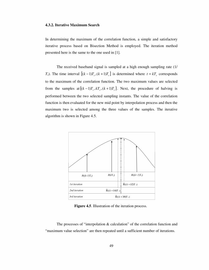
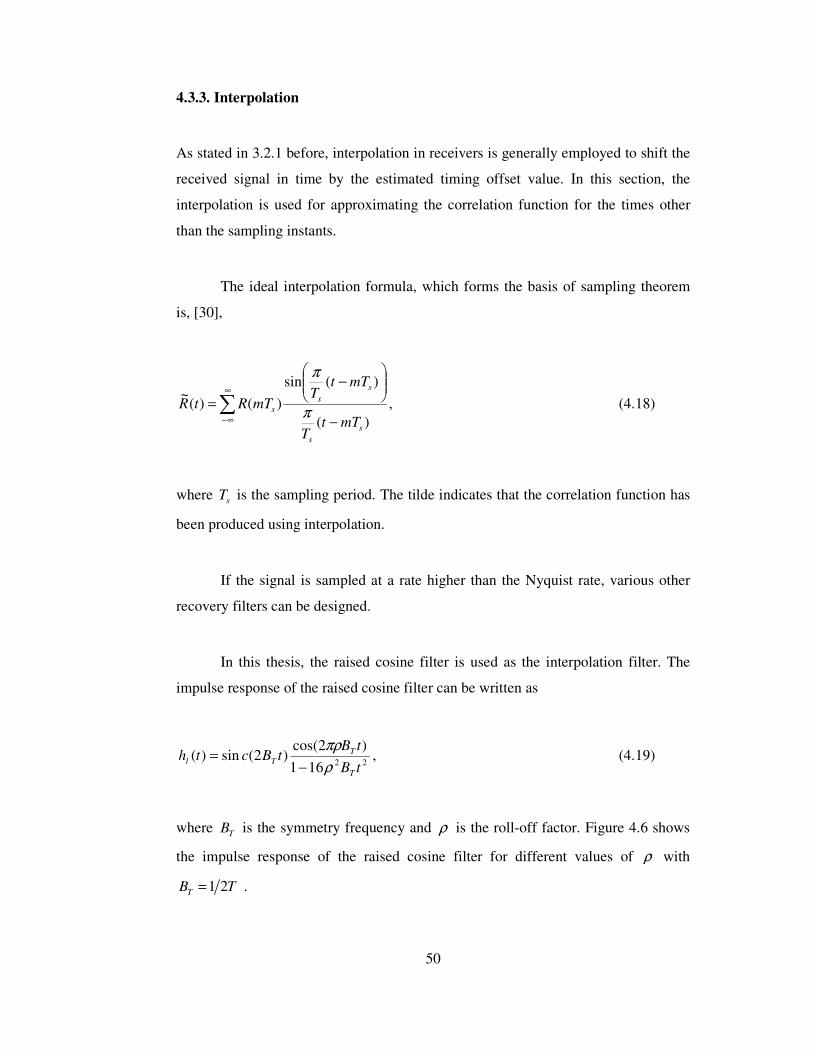
SYMBOL TIMING RECOVERY FOR CPM SIGNALS BASED ON MATCHED FILTERING A THESIS SUBMITTED TO THE GRADUATE SCHOOL OF NATURAL AND APPLIED SCIENCES OF MIDDLE EAST TECHNICAL UNIVERSITY BY ÇİLER BAŞERDEM IN PARTIAL FULFILLMENT OF THE REQUIREMENTS FOR THE DEGREE OF MASTER OF SCIENCE IN THE DEPARTMENT OF ELECTRICAL AND ELECTRONICS ENGINEERING DECEMBER 2006
Transcript
SYMBOL TIMING RECOVERY FOR CPM SIGNALS BASED ON MATCHED FILTERING
A THESIS SUBMITTED TO THE GRADUATE SCHOOL OF NATURAL AND APPLIED SCIENCES
OF MIDDLE EAST TECHNICAL UNIVERSITY
BY
ÇİLER BAŞERDEM
IN PARTIAL FULFILLMENT OF THE REQUIREMENTS FOR
THE DEGREE OF MASTER OF SCIENCE IN
THE DEPARTMENT OF ELECTRICAL AND ELECTRONICS ENGINEERING
DECEMBER 2006
Approval of the Graduate School of Natural and Applied Sciences
Prof. Dr. Canan Özgen Director
I certify that this thesis satisfies all the requirements as a thesis for the degree of Master of Science.
Prof. Dr. İsmet Erkmen Head of Department
This is to certify that we have read this thesis and that in our opinion it is fully adequate, in scope and quality, as a thesis for the degree of Master of Science.
Prof. Dr. Yalçın Tanık Supervisor Examining Committee Members Prof. Dr. Mete Severcan (METU, EE)
Prof. Dr. Yalçın Tanık (METU, EE)
Prof. Dr. Kerim Demirbaş (METU, EE)
Assist. Prof. Dr. Ali Özgür Yılmaz (METU, EE)
Çağdaş Enis Doyuran ( M.S.) (ASELSAN)
iii
I hereby declare that all information in this document has been obtained and presented in accordance with academic rules and ethical conduct. I also declare that, as required by these rules and conduct, I have fully cited and referenced all material and results that are not original to this work. Name, Last name : Çiler Başerdem
Signature :
iv
ABSTRACT
SYMBOL TIMING RECOVERY FOR CPM SIGNALS
BASED ON MATCHED FILTERING
Başerdem, Çiler
M.S., Department of Electrical and Electronics Engineering
Supervisor : Prof. Dr. Yalçın Tanık
December 2006, 96 pages
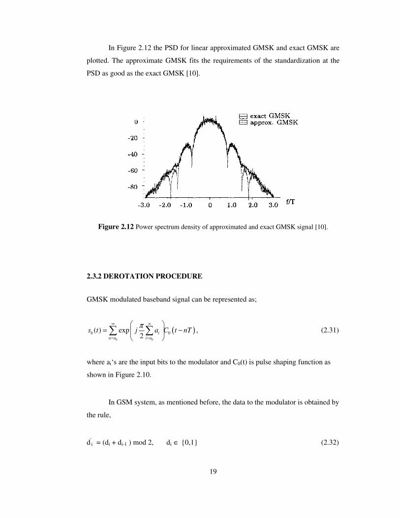
In this thesis, symbol timing recovery based on matched filtering in Gaussian
Minimum Shift Keying (GMSK) with bandwidth-bit period product (BT) of 0.3 is
investigated. GMSK is the standard modulation type for GSM. Although GMSK
modulation is non-linear, it is approximated to Offset Quadrature Amplitude
Modulation (OQAM), which is a linear modulation, so that Maximum Likelihood
Sequence Estimation (MLSE) method is possible in the receiver part. In this study
Typical Urban (TU) channel model developed in COST 207 is used. Two methods
are developed on the construction of the matched filter. In order to obtain timing
recovery for GMSK signals, these methods are investigated. The fractional time
delays are acquired by using interpolation and an iterative maximum search process.
The performance of the proposed symbol timing recovery (STR) scheme is assessed
by using computer simulations. It is observed that the STR tracks the variations of
the frequency selective multipath fading channels almost the same as the Mazo
criterion.
v
Keywords: Symbol timing recovery, Gaussian Minimum Shift Keying (GMSK),
matched filtering, multipath fading channel, Mazo criterion.
vi
ÖZ
CPM SİNYALLERİ İÇİN UYUMLU SÜZGEÇLEMEYE DAYALI SEMBOL ZAMAN BİLGİSİNİN KAZANIMI
Başerdem, Çiler
Yüksek Lisans, Elektrik ve Elektronik Mühendisliği Bölümü
Tez Yöneticisi : Prof. Dr. Yalçın Tanık
Aralık 2006, 96 sayfa
Bu tezde, bant genişliği ile bit aralığı çarpımı 0.3 olan Gaussian en küçük
kaydırmalı kiplenim (GMSK) sinyalleri için uyumlu süzgeçlemeye dayalı sembol
zaman bilgisinin kazanımı incelenmiştir. GMSK, GSM sistemi için standart
modülasyon tipidir. GMSK modülasyonu, doğrusal olmamasına rağmen, en büyük
olasılıklı dizi kestirimi (MLSE) yönteminin alıcı kısmında kullanılabilmesi için
doğrusal bir modülasyon tipi olan OQAM’ ye benzetilmiştir. Bu çalışmada COST
207 ‘de geliştirilen şehiriçi tipik kanal modeli kullanılmıştır. Uyumlu süzgeç yapısı
için iki yöntem geliştirilmiştir. GMSK sinyalleri için zaman bilgisinin kazanımını
elde etmek amacıyla bu iki yöntem incelenmiştir. Ufak zaman gecikmeleri,
aradeğerleme ve döngülü en yüksek arama yöntemleri kullanılarak elde edilmiştir.
Önerilen sembol zaman kazanım (STR) yapısının başarımı bilgisayar benzetimleri
kullanılarak değerlendirilmiştir. STR’nin frekans seçici çokyönlü sönümlemeli kanal
değişimlerini Mazo ölçütüne çok benzer takip ettiği gözlenmiştir.
vii
Anahtar kelimeler: Sembol zaman kazanımı, Gaussian en küçük kaydırmalı
kiplenim , uyumlu süzgeç, çokyönlü sönümlemeli kanal, Mazo ölçütü.
viii
To my family
ix
ACKNOWLEDGMENTS
I would like to express my appreciation to my supervisor Prof. Dr. Yalçın Tanık for
his supervision, support and helpful comments on this thesis.
I am also grateful to ASELSAN Inc. for letting and supporting of my thesis.
Additionally I would like to thank to Çağdaş Enis Doyuran for his motivative
comments and great contributions about writing this thesis.
I also wish to express my deep gratitude to my parents and my dear brother, for their
support during my life.
Finally, special thanks are due to my colleague Hazım Tokuçcu for his great support,
encouragement and patience throughout my thesis study.
B.APPROXIMATION OF GMSK TO LINEAR QAM SIGNAL............................92
xiii
LIST OF TABLES
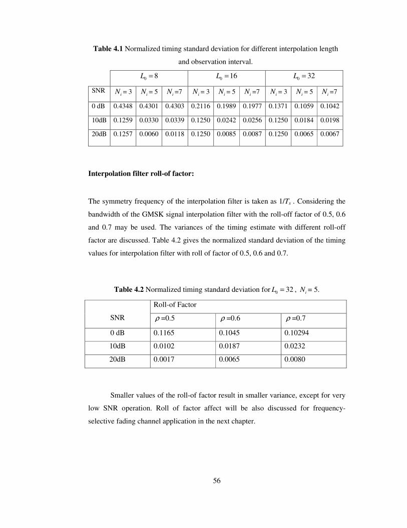
TABLES Table 2.1 Training sequence codes ………………………………………………… 24 Table 4.1 Normalized timing standard deviation for different interpolation length
and observation interval……..…………....................................................56 Table 4.2 Normalized timing standard deviation for Lo=32, Ni = 5…………….......56 Table 5.1 The rms error values for the simulations in Figure 5.9 and 5.10………....67 Table 5.2 The rms error values for the simulations in Figure 5.11 and 5.12……..…68 Table 5.3 The rms error values for the simulations in Figure 5.15
and 5.16…………………………………………….……………………..72 Table 5.4 The rms error values for the simulations in Figure 5.17………………….74 Table 5.5 The rms error values for the simulations in Figure 5.18……………….....74 Table 5.6 The rms error values for the simulations in Figure 5.19 and 5.20………..76 Table 5.7 The rms error values for the simulations in Figure 5.21…….…………....78 Table 5.8 The rms error values for the simulations in Figure 5.22………………….78
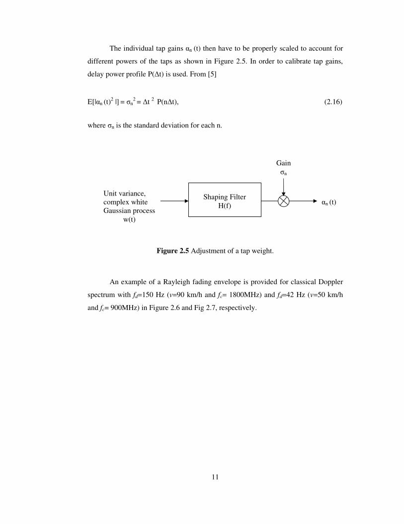
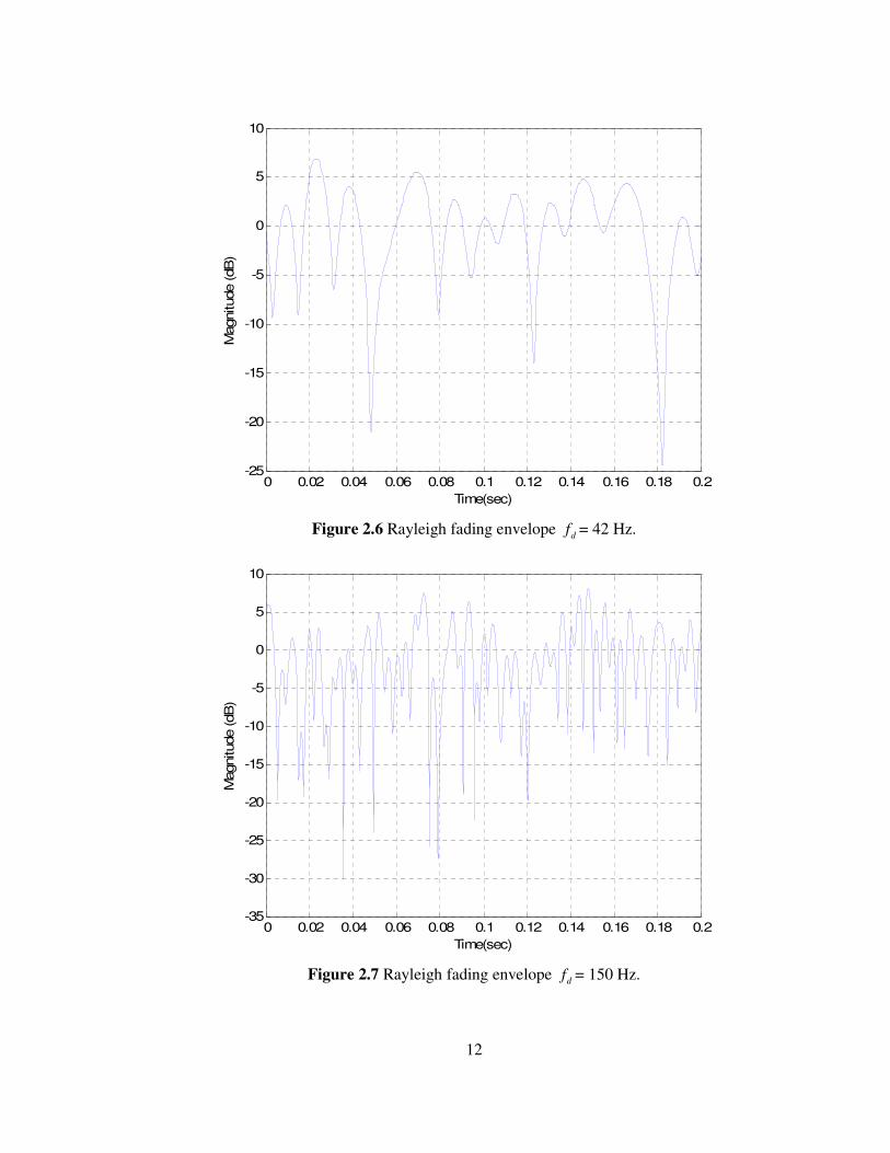
Figure 2.3 Power delay profile for Typical Urban (TU) channel……..……………...9 Figure 2.4 Filtering of white noise……………………………..……………………10 Figure 2.5 Adjustment of a tap weight………………………...…………………….11 Figure 2.6 Rayleigh fading envelope
df = 42 Hz………….……………..……….…12
Figure 2.7 Rayleigh fading envelope
df = 150 Hz…….…………………………….12
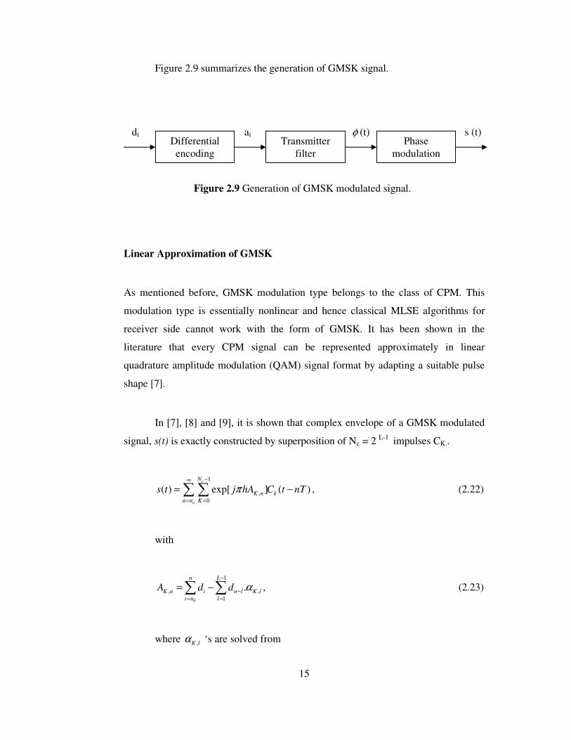
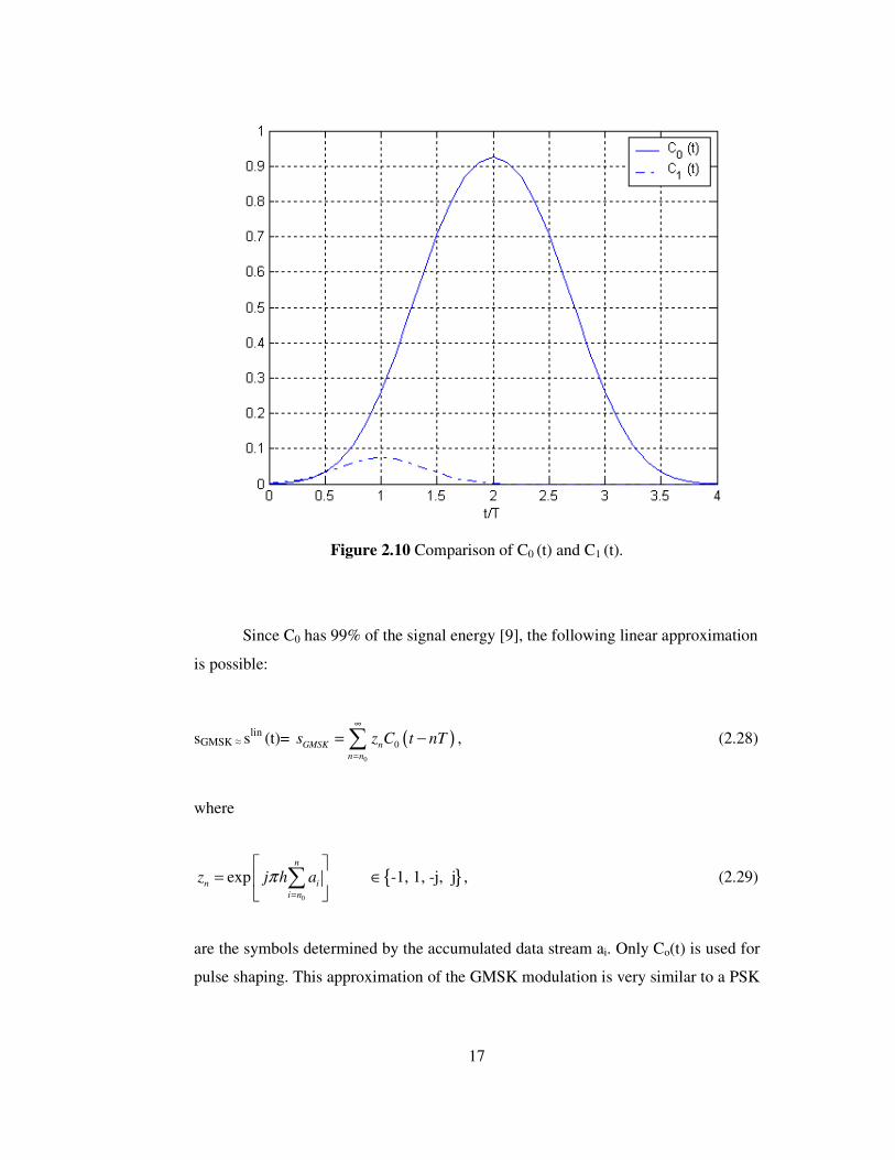
Figure 2.8 Baseband shaping pulse of g(t)…………………………….……………14 Figure 2.9 Generation of GMSK modulated signal………………….……………...15 Figure 2.10 Comparison of C0 (t) and C1 (t)………………………………………....17 Figure 2.11 Complex envelope of approximated GMSK signal …….……………...18 Figure 2.12 Power spectrum density of approximated and exact GMSK
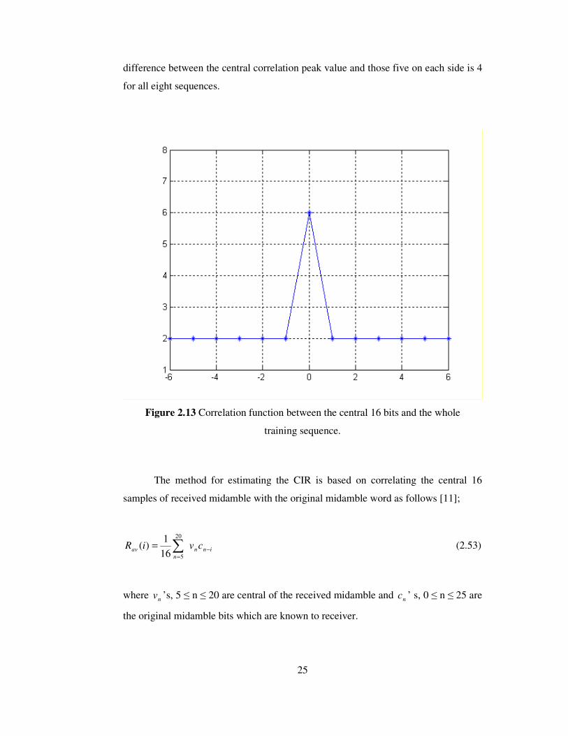
signal……….…………………………………………………………..19 Figure 2.13 Correlation function between the central 16 bits and the whole
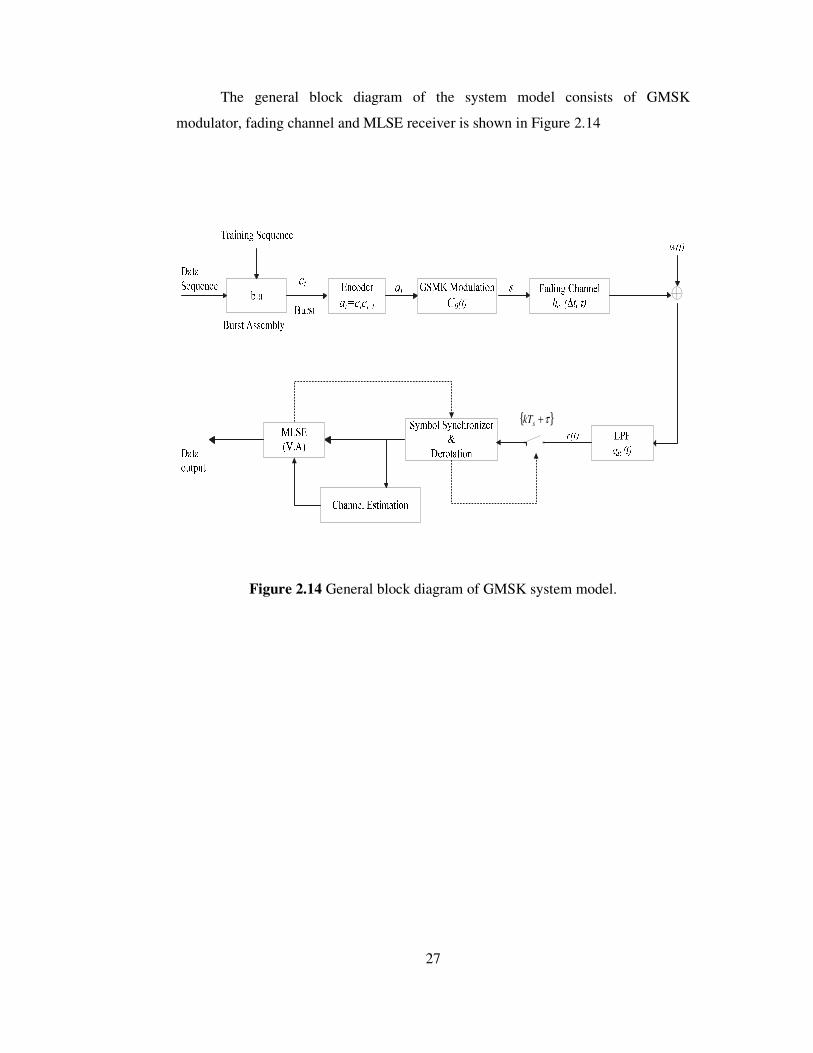
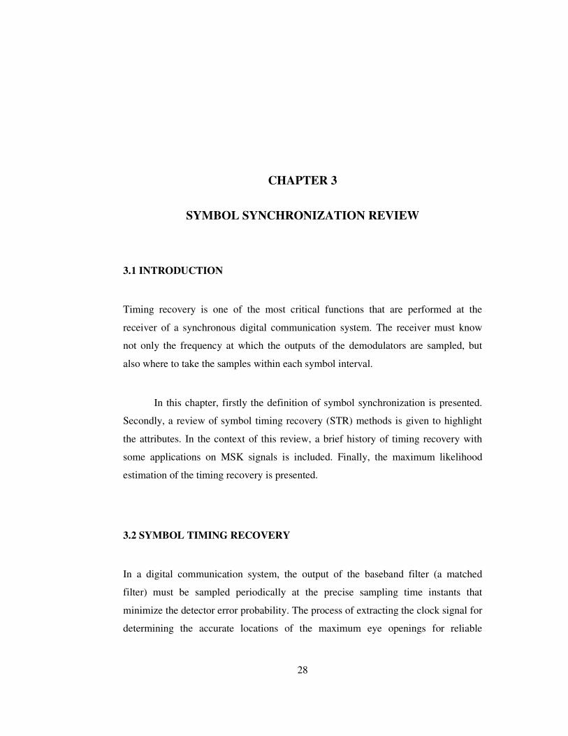
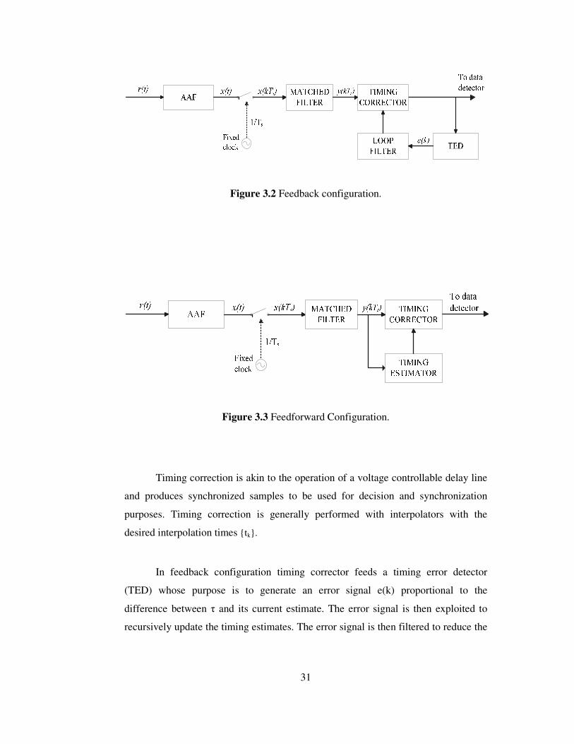
training sequence….……………..…………….………………………25 Figure 2.14 General block diagram of GMSK system model…………….………...27 Figure 3.1 Typical block diagram of a baseband receiver…………………………..29 Figure 3.2 Feedback configuration……………………………….………………....31
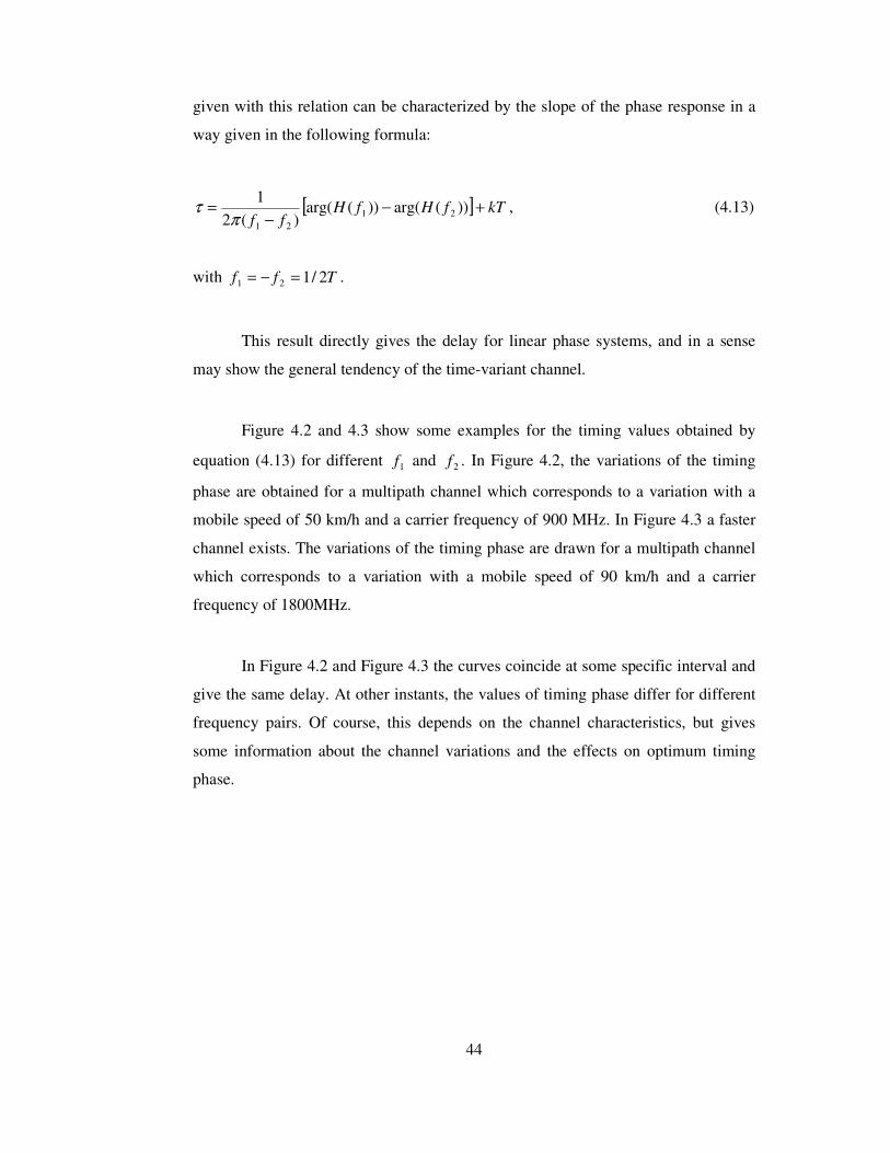
Figure 4.2 Normalized timing phase obtained from Mazo criterion (v=50 km/h,
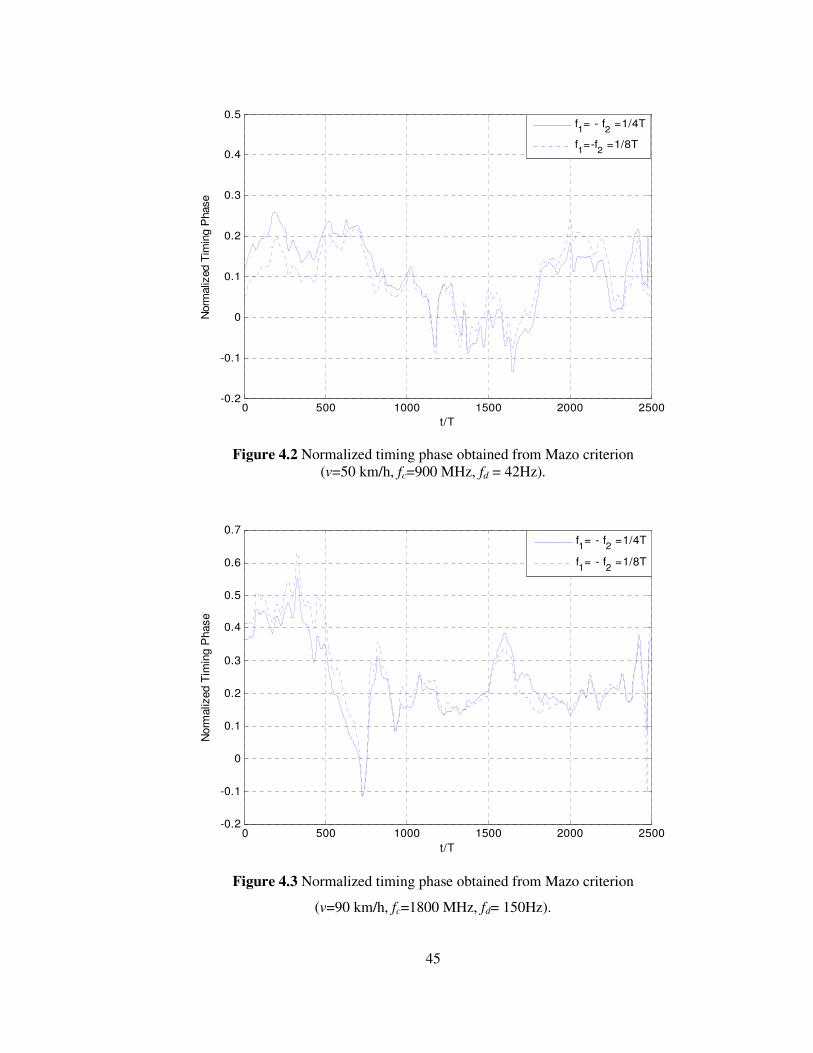
fc=900 MHz, fd = 42Hz)………………………………………………...45 Figure 4.3 Normalized timing phase obtained from Mazo criterion (v=90 km/h,
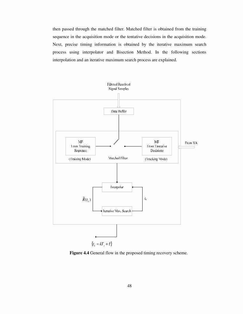
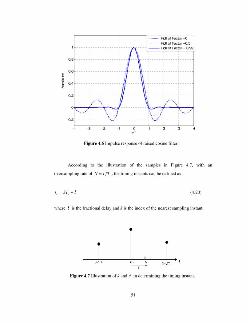
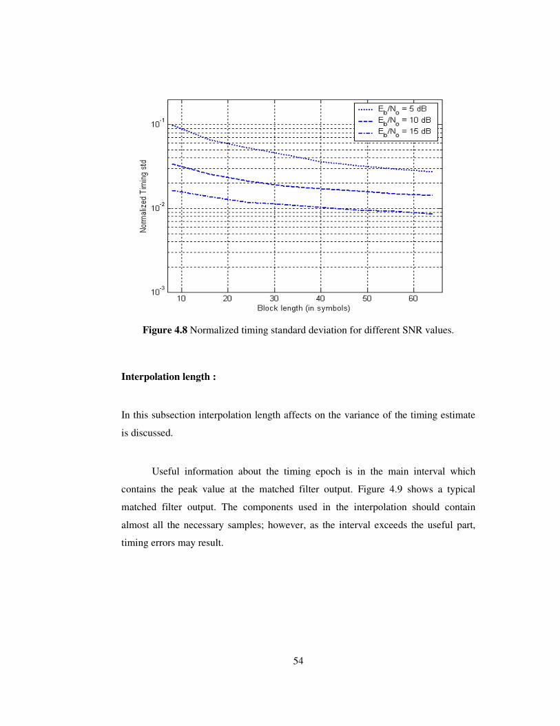
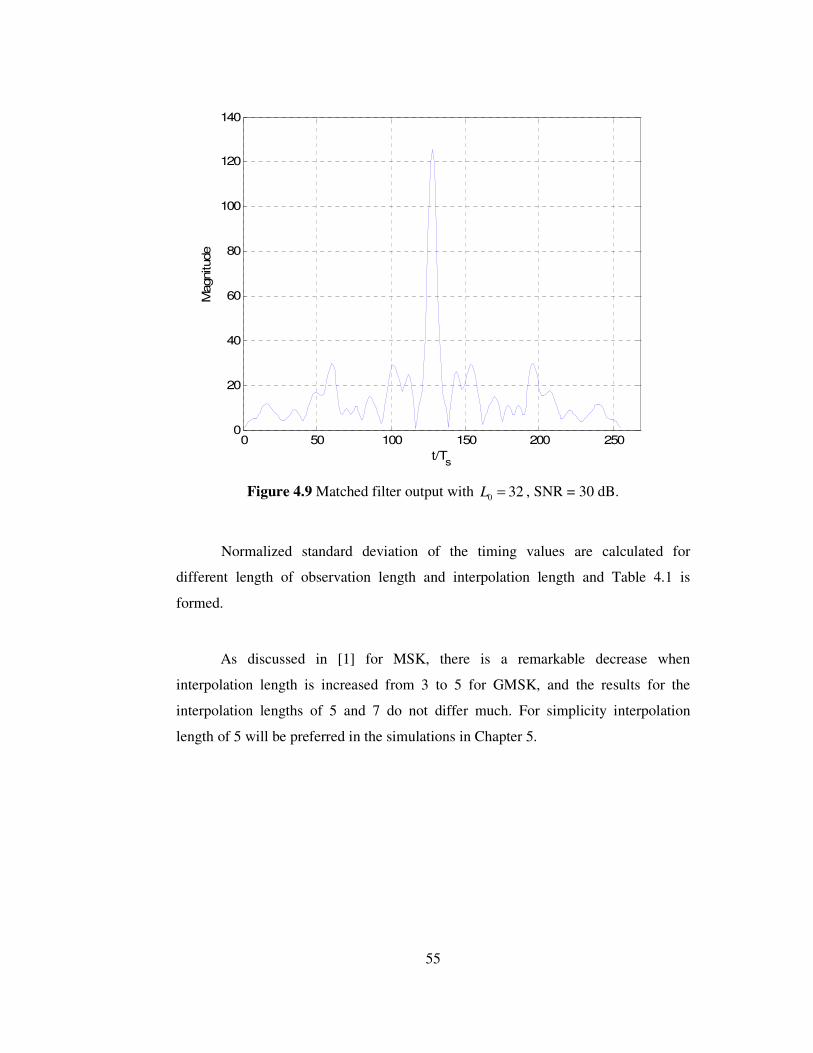
fc=1800 MHz, fd= 150Hz)…………………….………………………....45 Figure 4.4 General flow in the proposed timing recovery scheme…………………48 Figure 4.5 Illustration of the iteration process……………………………………...49 Figure 4.6 Impulse response of raised cosine filter………………………………....51 Figure 4.7 Illustration of k and τ in determining the timing instant……………….52 Figure 4.8 Normalized timing standard deviation for different SNR values………..54 Figure 4.9 Matched filter output with 0 32L = , SNR = 30 dB……………………...55
Figure 5.1 General block diagram of the simulated system………….………….….59 Figure 5.2 Complex envelope of the approximated GMSK signal……………....…60 Figure 5.3 Power spectrum density of linear GMSK and exact GMSK signal.….....60 Figure 5.4 Tapped delay line model of the multipath fading channel…….…….......61 Figure 5.5 Generation of taps……………………….…………………………...….62 Figure 5.6 Location of )(tsi
………………………………………………………...64
Figure 5.7 Construction of the reference signal by Method A…...……………....…65 Figure 5.8 Construction of the reference signal by Method B. ……...…...………...65 Figure 5.9 Comparison of the Methods A and B ( oL =16 , SNR=30dB,
v=50 km/h and fc= 900MHz )...…..…..…………………………….…...66 Figure 5.10 Comparison of the Methods A and B ( oL =32 , SNR=30dB,
v=50 km/h and fc= 900MHz )…...……….……………………………...67
xvi
Figure 5.11 Comparison of the Methods A and B ( oL =16 , SNR=30dB,
v=90 km/h and fc= 1800MHz )………...……………………….……….68 Figure 5.12 Comparison of the Methods A and B ( oL =32 , SNR=30dB,
v=90 km/h and fc= 1800MHz )…………….…………..…………….….69 Figure 5. 13 Performance of the symbol synchronizer for oL =16……………...…..70
Figure 5.14 Performance of the symbol synchronizer for oL =32…………………..71
Figure 5.15 Tracking performance of the proposed synchronizer for two
observation intervals (SNR=30dB, v=50 km/h and fc= 900MHz )...........73 Figure 5.16 Tracking performance of the proposed synchronizer for two
observation intervals (SNR=30dB, v=50 km/h and fc= 900MHz )……...73 Figure 5.17 Tracking performance of the proposed synchronizer for different roll
of factor values ( oL =32, SNR=30dB, v=50 km/h and fc= 900MHz )......75
Figure 5.18 Tracking performance of the proposed synchronizer for different SNR
values ( oL =32, v=50 km/h and fc= 900MHz )……………………….…75
Figure 5.19 Tracking performance of the proposed synchronizer for two observation
intervals (SNR=30dB, v=90 km/h and fc= 1800MHz )…………………77 Figure 5.20 Tracking performance of the proposed synchronizer for two observation
intervals (SNR=30dB, v=90 km/h and fc= 1800MHz )…………………77 Figure 5.21 Tracking performance of the proposed synchronizer for different roll
of factor values ( oL =32, SNR=30dB, v=90 km/h and fc= 1800MHz )…79
Figure 5.22 Tracking performance of the proposed synchronizer for different SNR
values ( oL =32, v=90 km/h and fc= 1800MHz )………………………...79
xvii
LIST OF ABBREVIATIONS
BT Bandwidth-Bit Period Product
BU Bad Urban
CIR Channel Impulse Response
CPM Continuous Phase Modulation
CRB Cramer Rao Bound
DA Data-aided
DD Decision-Directed
DECT Digital enhanced cordless telephone
GMSK Gaussian Minimum Shift Keying
GSM Global Systems Mobile Communications
HT Hilly Terrain
ISI Intersymbol Interference
LLF Log Likelihood Function
MCRB Modified Cramer Rao Bound
ML Maximum Likelihood
MLSE Maximum Likelihood Sequence Estimation
MMSE Minimum Mean Square Estimation
msISI Minimum Squared Intersymbol Interference
MSK Minimum Shift Keying
NCO Number Controlled Oscillator
xviii
NDA Non-Data Aided
NDD Non-Decision Directed
OQAM Offset Quadrature Amplitude Modulation
RA Rural Area
STR Symbol Timing Recovery
TED Timing Error Detector
TSC Training Sequence Code
TU Typical Urban
1
CHAPTER 1
INTRODUCTION
1.1 SCOPE AND OBJECTIVE
Symbol synchronization or symbol timing recovery is a crucial part of the receiver in
synchronous communication systems. The timing information depends on the overall
system impulse response thus, on the characteristics of the communication channel.
Most of the practical synchronizers have been based on transmission systems with no
intersymbol interference (ISI) or with a time spread less than a symbol period, which
is not realistic at all. On the other hand, multipath fading channel with a large delay
spread causes ISI, so determination of the sampling instant is a much more difficult
problem. Therefore transmission over frequency-selective fading channels
necessitates specifically designed synchronizer structures and algorithms.
Feedforward approaches based on maximum likelihood estimation are good
candidates because of their rapid acquisition of symbol timing with the absence of
hang-up problems, which are very common for feedback configurations.
Symbol timing recovery of continuous phase modulation (CPM) signals has
taken considerable attention due to the attractive characteristics of the signal. CPM is
a constant envelope, nonlinear modulation method which conserves and reduces
energy and bandwidth at the same time. Minimum shift keying (MSK) and Gaussian
minimum shift keying (GMSK) are the special forms of CPM. The modulation
scheme chosen by GSM is GMSK with a bandwidth symbol period product of
BT=0.3. Also GMSK with BT=0.5 is the modulation of the DECT system.
2
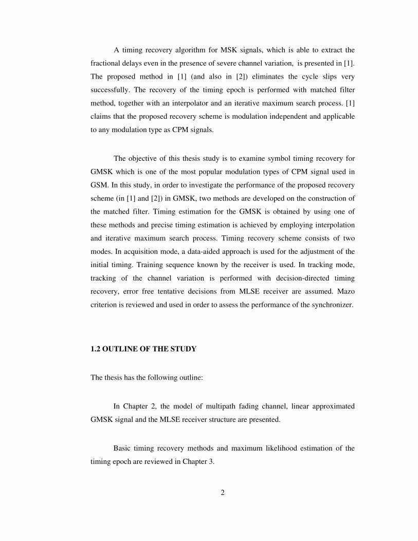
A timing recovery algorithm for MSK signals, which is able to extract the
fractional delays even in the presence of severe channel variation, is presented in [1].
The proposed method in [1] (and also in [2]) eliminates the cycle slips very
successfully. The recovery of the timing epoch is performed with matched filter
method, together with an interpolator and an iterative maximum search process. [1]
claims that the proposed recovery scheme is modulation independent and applicable
to any modulation type as CPM signals.
The objective of this thesis study is to examine symbol timing recovery for
GMSK which is one of the most popular modulation types of CPM signal used in
GSM. In this study, in order to investigate the performance of the proposed recovery
scheme (in [1] and [2]) in GMSK, two methods are developed on the construction of
the matched filter. Timing estimation for the GMSK is obtained by using one of
these methods and precise timing estimation is achieved by employing interpolation
and iterative maximum search process. Timing recovery scheme consists of two
modes. In acquisition mode, a data-aided approach is used for the adjustment of the
initial timing. Training sequence known by the receiver is used. In tracking mode,
tracking of the channel variation is performed with decision-directed timing
recovery, error free tentative decisions from MLSE receiver are assumed. Mazo
criterion is reviewed and used in order to assess the performance of the synchronizer.
1.2 OUTLINE OF THE STUDY
The thesis has the following outline:
In Chapter 2, the model of multipath fading channel, linear approximated
GMSK signal and the MLSE receiver structure are presented.
Basic timing recovery methods and maximum likelihood estimation of the
timing epoch are reviewed in Chapter 3.
3
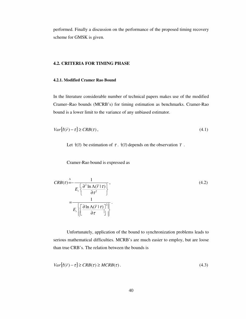
In Chapter 4, important tools; modified Cramer-Rao bound and one of the
possible criteria; Mazo criteria are presented in order to assess performance of the
synchronizer. Then, the proposed timing recovery scheme, consisting of correlation
method, interpolation and the iterative maximum search algorithm in [1], is
reviewed. Finally, parameters which affect the performance of the timing recovery
scheme are discussed.
The simulations and results are presented in Chapter 5. The simulated system
is described in detail. Methods developed on construction of the matched filter are
discussed which are special for GMSK application. Tracking ability of the proposed
timing scheme for GMSK is presented through the simulation results.
In the last chapter, conclusions and possible future work are presented.
The general form of the CPM signals and especially MSK and GMSK signals
are given in Appendix A.
In Appendix B, approximation of GMSK signal to linear QAM signal is
presented in detail.
4
CHAPTER 2
BACKGROUND MATERIAL
2.1 INTRODUCTION
In radio channels the received signal is the sum of a number of signals arriving
through different propagation paths. Each signal path is affected by a random
amplitude attenuation and a phase shift that tend to change over time. Due to the
multipath nature of the communication channel, interference occurs between
adjacent symbols, which is known as intersymbol interference (ISI). The maximum
likelihood sequence estimation (MLSE) technique has the best performance for
demodulating operations over channels with ISI and additive white Gaussian noise.
In this chapter model of multipath fading channels and MLSE receiver for
GMSK signals are presented.
2.2 CHANNEL MODEL
The mobile radio channel is based on the propagation of radio waves in a complex
transmission environment. For mobile radio applications, the channel is time-varying
because the motion between the transmitter and receiver results in propagation path
changes.
5
2.2.1 Characterization of Multipath Fading Channel
From [1] the equivalent low-pass channel is expressed by time-variant response
( ; ) ( ) ( )c n n
n
h t t t t tα δ∆ = ∆ − ∆∑ , (2.1)
where hc (∆t;t) represents the response of the channel at time t due to an impulse
applied at time ∆t-t [3] The complex process, ( )n tα can be represented as
( ) ( ) c njw t
n nt c t eα − ∆= , (2.2)
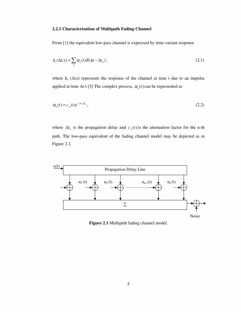
where nt∆ is the propagation delay and ( )nc t is the attenuation factor for the n-th
path. The low-pass equivalent of the fading channel model may be depicted as in
Figure 2.1.
Figure 2.1 Multipath fading channel model.
∑
α1 (t) α2 (t) αn-1(t) αn (t)
sl(t)
Noise
Propagation Delay Line
6
2.2.2 Channel Statistical Characterization:
The scattering function S(∆t;f) is the most important statistical measure of the
random multipath channel. It is a function of two variables; ∆t (delay) and a
frequency domain variable f is called the Doppler frequency. The scattering function
provides a single measure of the average power output of the channel as a function of
the delay ∆t and the f Doppler frequency. In other words, the scattering function
describes the manner in which the transmitted power is distributed in time and
frequency, upon passing through the channel. From the scattering function we can
obtain some of the most important relationships of a channel which impact the
performance of a communication system operating over that channel.
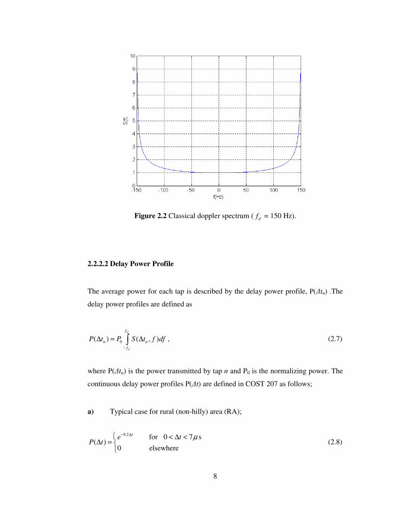
The delay-power profile P (∆t), which is also referred to as the multipath
intensity profile, is related to the scattering function via
( ) ( , )P t S t f df
∞
−∞
∆ = ∆∫ . (2.3)
Another function that is useful in characterizing fading is the Doppler power
spectrum, which is derived from the scattering function through
( ) ( , )S f S t f d t
∞
−∞
= ∆ ∆∫ . (2.4)
Different propagation models can be described by defining discrete number
of taps, each determined by their time delay and average power.
2.2.2.1 Doppler Power Spectrum
Doppler spectrum S(f) determines the time variations of the channel. When S(f) is
equal to the delta function , the channel becomes to be time-invariant.
7
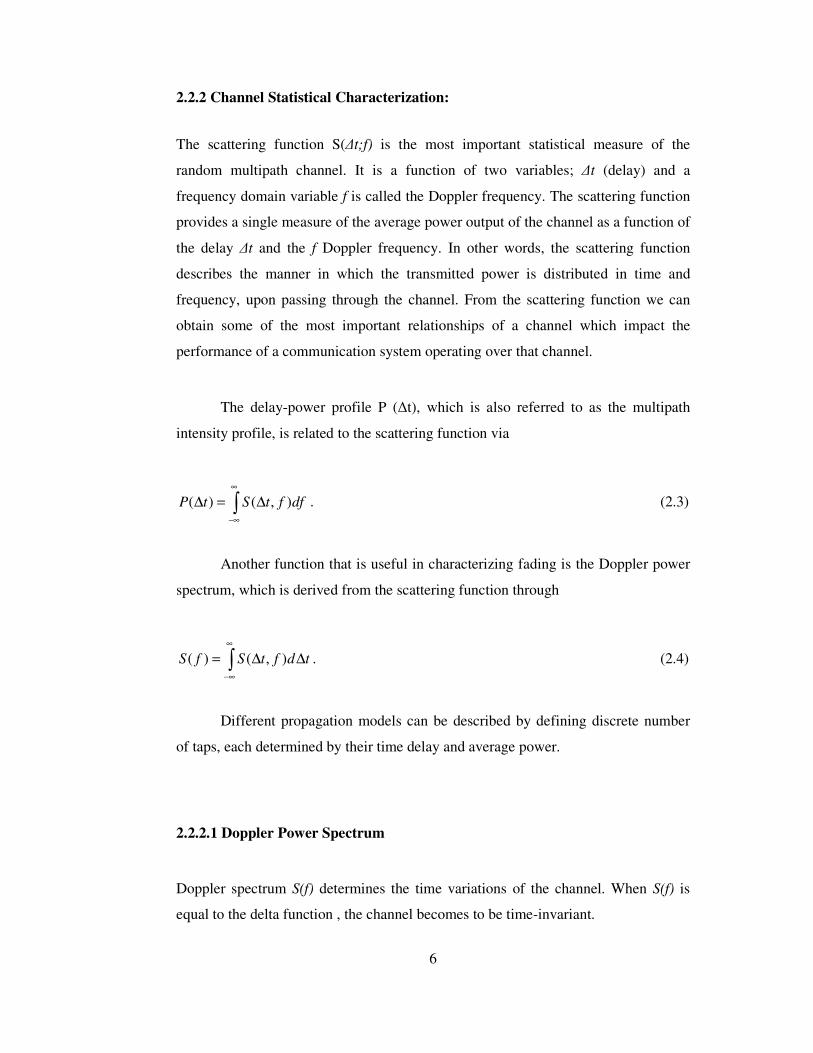
For modeling of the channel, three types of Doppler spectra is defined in
COST 207 final report; classical Doppler spectrum, Gauss 1 and Gauss 2 [4]. The
most commonly used, and in a certain sense, the worst case Doppler spectrum is the
classical Doppler spectrum which is also called Jakes spectrum. In this spectrum
type, all the angle between vehicle speed and radio wave are assumed to be equally
probable [5]. The classical Doppler spectrum
1/ 22( ) for (- , )
1 ( / )d d
d
AS f f f f
f f= ∈ −
, (2.5)
where fd is maximum Doppler shift, and
d c
vf f
c= ⋅ , (2.6)
where v is the velocity of the mobile and cf the carrier frequency. The classical
Doppler spectrum is used throughout this study.
Classical Doppler spectrum for a mobile speed of 90 km/h and a carrier
The symmetry frequency of the interpolation filter is taken as 1/Ts . Considering the
bandwidth of the GMSK signal interpolation filter with the roll-off factor of 0.5, 0.6
and 0.7 may be used. The variances of the timing estimate with different roll-off
factor are discussed. Table 4.2 gives the normalized standard deviation of the timing
values for interpolation filter with roll of factor of 0.5, 0.6 and 0.7.
Table 4.2 Normalized timing standard deviation for 0 32L = , iN = 5.
Roll-of Factor
SNR ρ =0.5 ρ =0.6 ρ =0.7
0 dB 0.1165 0.1045 0.10294
10dB 0.0102 0.0187 0.0232
20dB 0.0017 0.0065 0.0080
Smaller values of the roll-of factor result in smaller variance, except for very
low SNR operation. Roll of factor affect will be also discussed for frequency-
selective fading channel application in the next chapter.
57
CHAPTER 5
SIMULATION AND RESULTS
5.1 INTRODUCTION
The proposed decision-directed symbol synchronizer model has been developed in
MATLAB. Although MATLAB is based on discrete time signals, the continuous-
time signals are represented by their discrete samples taken at a rate much greater
than the Nyquist rate for a proper simulation.
In this chapter, firstly the model of the simulated system is presented. Next,
several properties of the GMSK modulated signal, the channel model and channel tap
generation process and methods of construction on the matched filter are discussed.
Performance of the symbol synchronizer in AWGN channel is compared with
MCRB for different observation intervals. Finally, the tracking performance of the
synchronizer is compared with Mazo criterion.
5.2 SIMULATION MODEL OF THE COMMUNICATION SYSTEM
The signal processing in the simulations is realized in baseband. The general
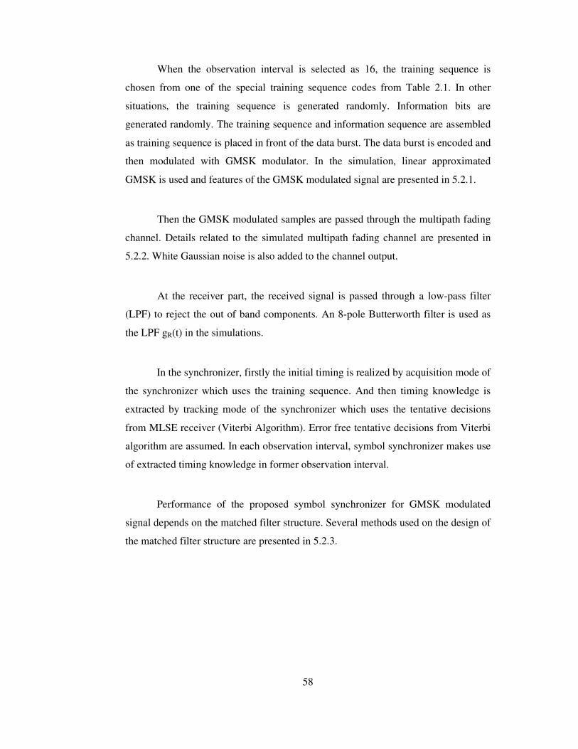
simulated diagram is shown in Figure 5.1.
58
When the observation interval is selected as 16, the training sequence is
chosen from one of the special training sequence codes from Table 2.1. In other
situations, the training sequence is generated randomly. Information bits are
generated randomly. The training sequence and information sequence are assembled
as training sequence is placed in front of the data burst. The data burst is encoded and
then modulated with GMSK modulator. In the simulation, linear approximated
GMSK is used and features of the GMSK modulated signal are presented in 5.2.1.
Then the GMSK modulated samples are passed through the multipath fading
channel. Details related to the simulated multipath fading channel are presented in
5.2.2. White Gaussian noise is also added to the channel output.
At the receiver part, the received signal is passed through a low-pass filter
(LPF) to reject the out of band components. An 8-pole Butterworth filter is used as
the LPF gR(t) in the simulations.
In the synchronizer, firstly the initial timing is realized by acquisition mode of
the synchronizer which uses the training sequence. And then timing knowledge is
extracted by tracking mode of the synchronizer which uses the tentative decisions
from MLSE receiver (Viterbi Algorithm). Error free tentative decisions from Viterbi
algorithm are assumed. In each observation interval, symbol synchronizer makes use
of extracted timing knowledge in former observation interval.
Performance of the proposed symbol synchronizer for GMSK modulated
signal depends on the matched filter structure. Several methods used on the design of
the matched filter structure are presented in 5.2.3.
59
{ }τ+skT
Figure 5.1 General block diagram of the simulated system.
5.2.1 GMSK Modulated Signal
Linear approximation of the GMSK signal in equation (2.27) is used in the
simulations. Features of the simulated GMSK signal with BT of 0.3 are tested in
order to make sure validity of the modulated signal.
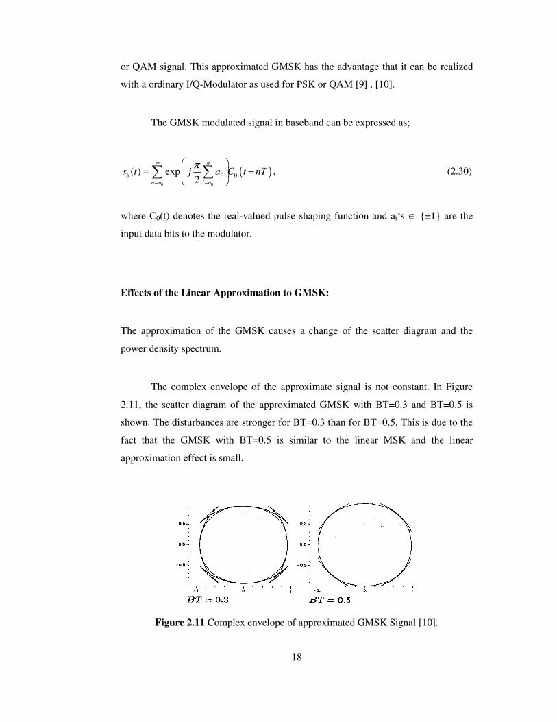
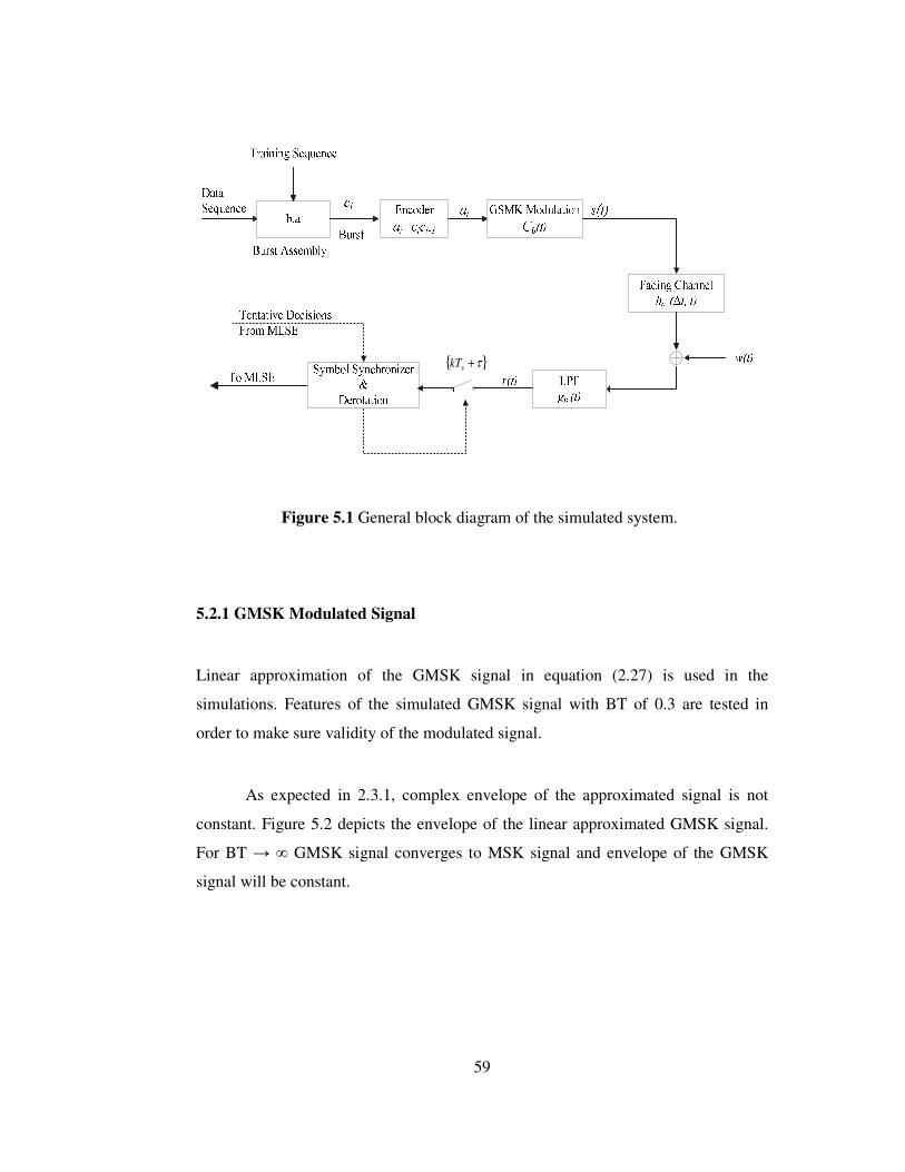
As expected in 2.3.1, complex envelope of the approximated signal is not
constant. Figure 5.2 depicts the envelope of the linear approximated GMSK signal.
For BT → ∞ GMSK signal converges to MSK signal and envelope of the GMSK
signal will be constant.
60
Figure 5.2 Complex envelope of the approximated GMSK signal.
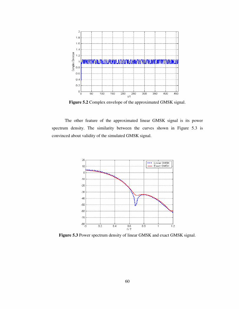
The other feature of the approximated linear GMSK signal is its power
spectrum density. The similarity between the curves shown in Figure 5.3 is
convinced about validity of the simulated GMSK signal.
Figure 5.3 Power spectrum density of linear GMSK and exact GMSK signal.
61
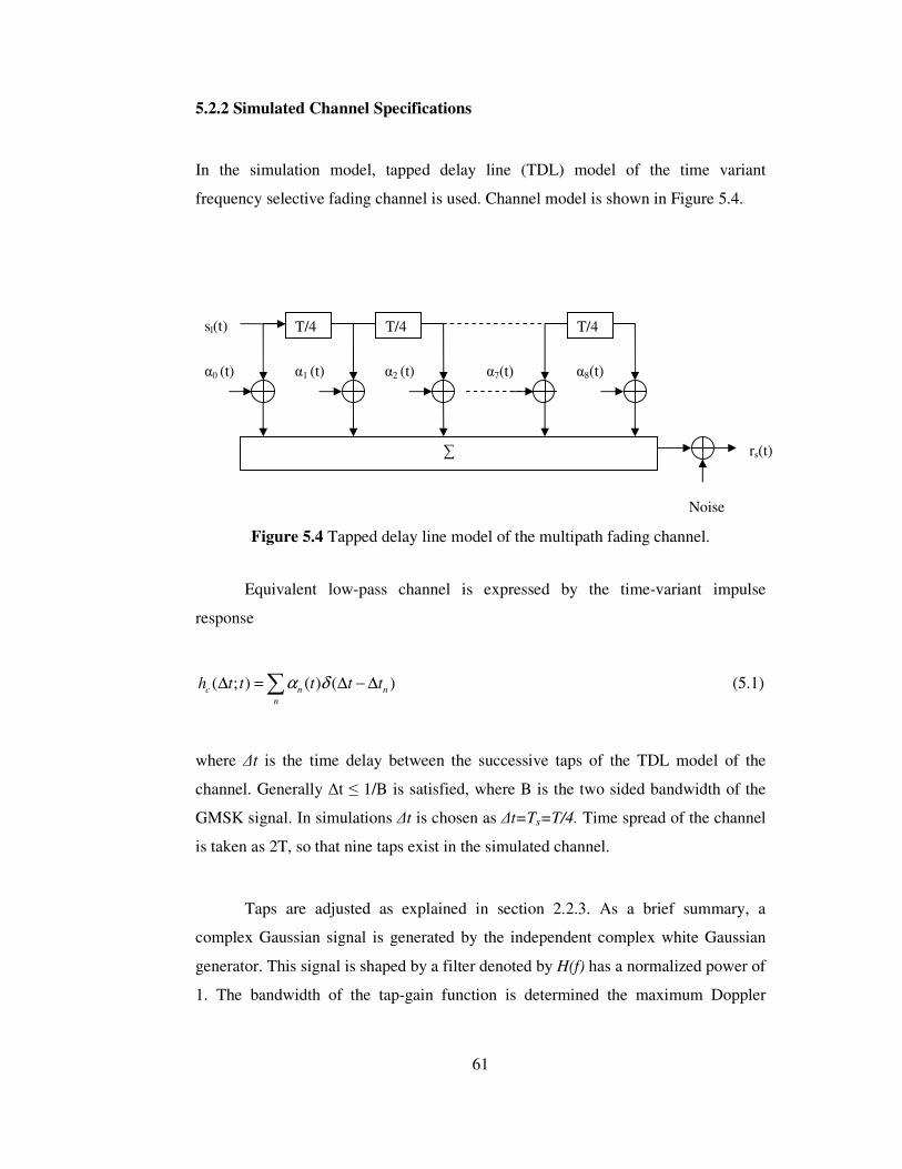
5.2.2 Simulated Channel Specifications
In the simulation model, tapped delay line (TDL) model of the time variant
frequency selective fading channel is used. Channel model is shown in Figure 5.4.
Figure 5.4 Tapped delay line model of the multipath fading channel.
Equivalent low-pass channel is expressed by the time-variant impulse
response
( ; ) ( ) ( )c n n
n
h t t t t tα δ∆ = ∆ − ∆∑ (5.1)
where ∆t is the time delay between the successive taps of the TDL model of the
channel. Generally ∆t ≤ 1/B is satisfied, where B is the two sided bandwidth of the
GMSK signal. In simulations ∆t is chosen as ∆t=Ts=T/4. Time spread of the channel
is taken as 2T, so that nine taps exist in the simulated channel.
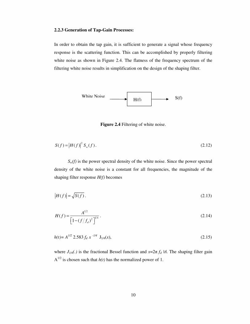
Taps are adjusted as explained in section 2.2.3. As a brief summary, a
complex Gaussian signal is generated by the independent complex white Gaussian
generator. This signal is shaped by a filter denoted by H(f) has a normalized power of
1. The bandwidth of the tap-gain function is determined the maximum Doppler
T/4 T/4 T/4
∑
α0 (t) α1 (t) α2 (t) α7(t) α8(t)
sl(t)
Noise
rs(t)
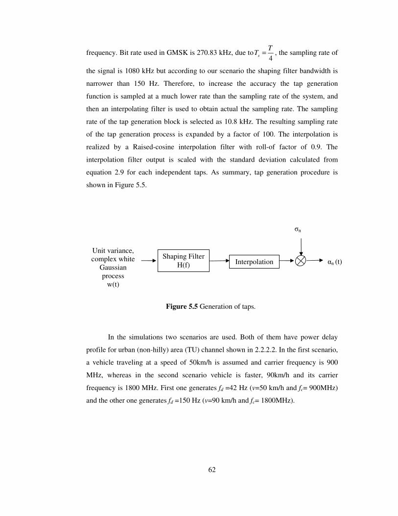
62
frequency. Bit rate used in GMSK is 270.83 kHz, due to4s
TT = , the sampling rate of
the signal is 1080 kHz but according to our scenario the shaping filter bandwidth is
narrower than 150 Hz. Therefore, to increase the accuracy the tap generation
function is sampled at a much lower rate than the sampling rate of the system, and
then an interpolating filter is used to obtain actual the sampling rate. The sampling
rate of the tap generation block is selected as 10.8 kHz. The resulting sampling rate
of the tap generation process is expanded by a factor of 100. The interpolation is
realized by a Raised-cosine interpolation filter with roll-of factor of 0.9. The
interpolation filter output is scaled with the standard deviation calculated from
equation 2.9 for each independent taps. As summary, tap generation procedure is
shown in Figure 5.5.
Figure 5.5 Generation of taps.
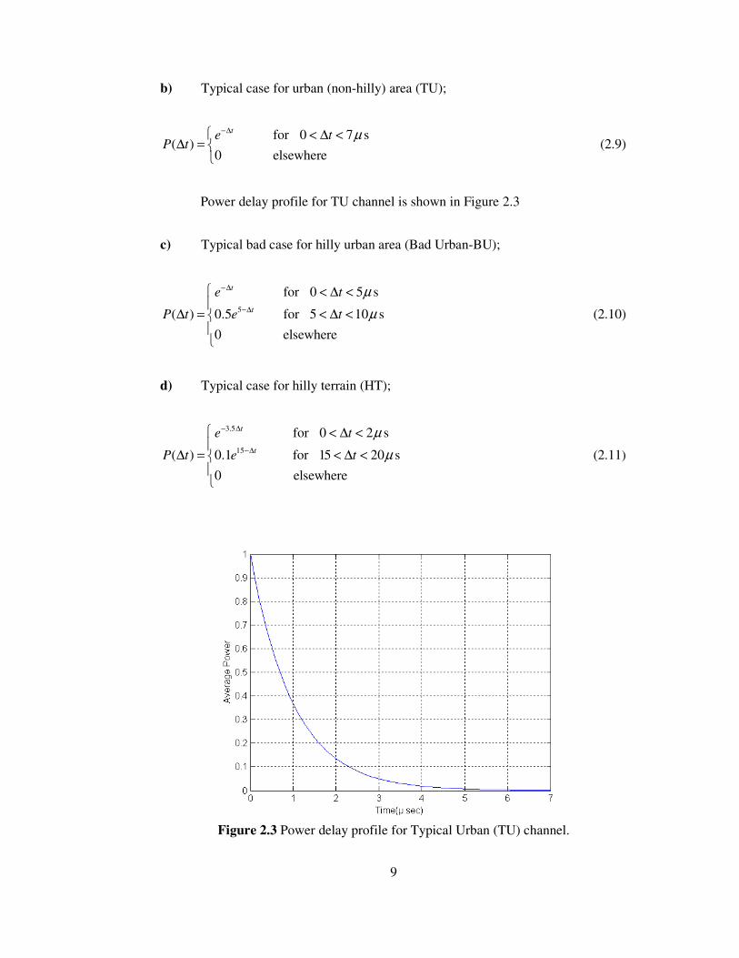
In the simulations two scenarios are used. Both of them have power delay
profile for urban (non-hilly) area (TU) channel shown in 2.2.2.2. In the first scenario,
a vehicle traveling at a speed of 50km/h is assumed and carrier frequency is 900
MHz, whereas in the second scenario vehicle is faster, 90km/h and its carrier
frequency is 1800 MHz. First one generates fd =42 Hz (v=50 km/h and fc= 900MHz)
and the other one generates fd =150 Hz (v=90 km/h and fc= 1800MHz).
Unit variance, complex white
Gaussian process
w(t)
Shaping Filter H(f) Interpolation
σn
αn (t)
63
5.2.3 Methods on the Matched Filter
The conclusive aim of a symbol synchronizer is to estimate the most likely value of
the timing epoch. In section 4.3.1 the correlation (matched filter) method was
discussed. The estimation of timing epoch is obtained by received signal passed
through the filter, which is matched to the reference signal over the observation
interval ( 0L ). This section presents two methods, called “Method A” and “Method
B”, on construction of the matched filter in other words the reference signal.
As explained in 4.3.1, in the acquisition mode a GMSK modulated signal
with the training sequence known by the receiver is used and in the tracking mode a
GMSK modulated signal with the tentative decisions, coming from MLSE receiver is
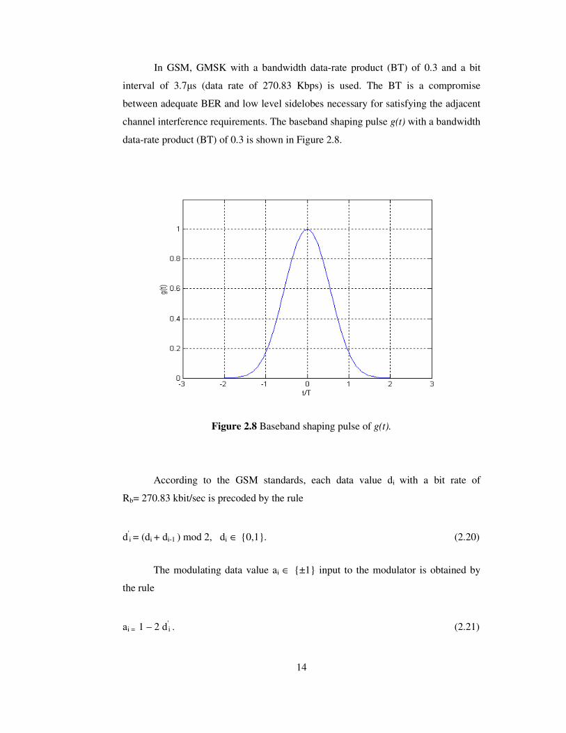
used. For the GMSK signal with BT=0.3, pulse shaping function g(t) in Figure 2.8
spans a time interval of approximately 4 symbol durations. Due to this, for the each
observation interval the GMSK modulated signal spans a time interval of 3 symbol
durations through the next observation interval. The last 3 symbol durations of the
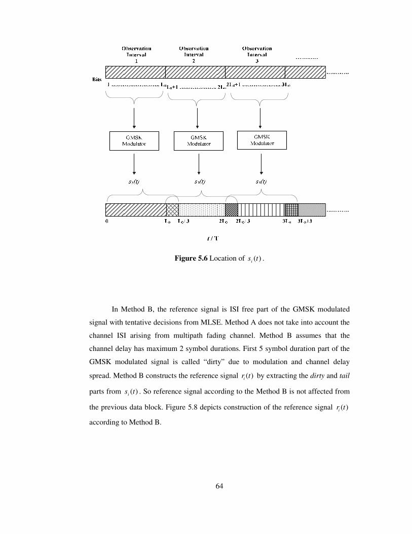
modulated signal is called as “tail”. For each observation interval GMSK modulated
signal denotes as )(tsi . Beginning and ending points of the )(tsi ’s are shown in
Figure 5.6.
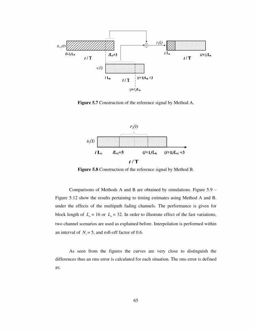
Method A constructs the reference signal by adding the first interval of 0L
symbol duration of the GMSK modulated signal of the currently observation interval
and last interval of 3 symbol duration of GMSK modulated signal from the previous
observation interval. Figure 5.7 depicts construction of the reference signal, ( )ir t by
Method A.
64
Figure 5.6 Location of )(tsi
.
In Method B, the reference signal is ISI free part of the GMSK modulated
signal with tentative decisions from MLSE. Method A does not take into account the
channel ISI arising from multipath fading channel. Method B assumes that the
channel delay has maximum 2 symbol durations. First 5 symbol duration part of the
GMSK modulated signal is called “dirty” due to modulation and channel delay
spread. Method B constructs the reference signal ( )ir t by extracting the dirty and tail
parts from )(tsi . So reference signal according to the Method B is not affected from
the previous data block. Figure 5.8 depicts construction of the reference signal ( )ir t
according to Method B.
65
Figure 5.7 Construction of the reference signal by Method A.
Figure 5.8 Construction of the reference signal by Method B.
Comparisons of Methods A and B are obtained by simulations. Figure 5.9 –
Figure 5.12 show the results pertaining to timing estimates using Method A and B.
under the effects of the multipath fading channels. The performance is given for
block length of oL = 16 or oL = 32. In order to illustrate effect of the fast variations,
two channel scenarios are used as explained before. Interpolation is performed within
an interval of iN = 5, and roll-off factor of 0.6.
As seen from the figures the curves are very close to distinguish the
differences thus an rms error is calculated for each situation. The rms error is defined
as;
66
∑=
=M
k
keM
E1
2)(1
, (5.2)
where e(k) is the difference between the normalized timing phase by Mazo criterion
and the normalized timing estimation from the synchronizer for each sampling
interval, M is the total number of sampling interval. In the simulations rms error
values are given in order to discuss performance with Method A and B for each
curve.
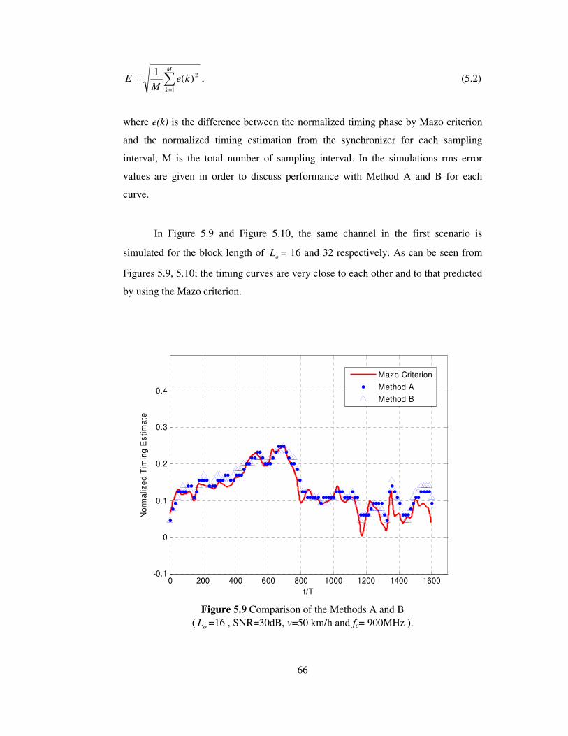
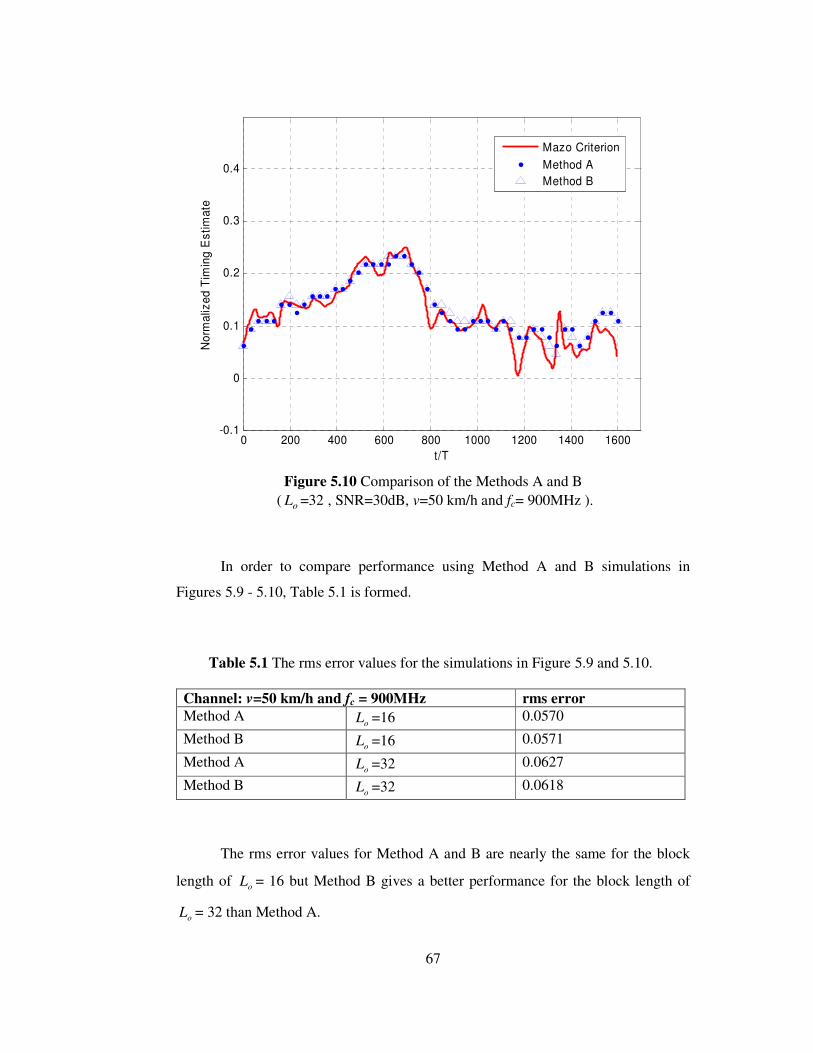
In Figure 5.9 and Figure 5.10, the same channel in the first scenario is
simulated for the block length of oL = 16 and 32 respectively. As can be seen from
Figures 5.9, 5.10; the timing curves are very close to each other and to that predicted
by using the Mazo criterion.
0 200 400 600 800 1000 1200 1400 1600-0.1
0
0.1
0.2
0.3
0.4
t/T
No
rma
lize
d T
imin
g E
sti
ma
te
Mazo Criterion
Method A
Method B
Figure 5.9 Comparison of the Methods A and B
( oL =16 , SNR=30dB, v=50 km/h and fc= 900MHz ).
67
0 200 400 600 800 1000 1200 1400 1600-0.1
0
0.1
0.2
0.3
0.4
t/T
No
rma
lize
d T
imin
g E
sti
ma
te
Mazo Criterion
Method A
Method B
Figure 5.10 Comparison of the Methods A and B
( oL =32 , SNR=30dB, v=50 km/h and fc= 900MHz ).
In order to compare performance using Method A and B simulations in
Figures 5.9 - 5.10, Table 5.1 is formed.
Table 5.1 The rms error values for the simulations in Figure 5.9 and 5.10.
Channel: v=50 km/h and fc = 900MHz rms error Method A
oL =16 0.0570
Method B oL =16 0.0571
Method A oL =32 0.0627
Method B oL =32 0.0618
The rms error values for Method A and B are nearly the same for the block
length of oL = 16 but Method B gives a better performance for the block length of
oL = 32 than Method A.
68
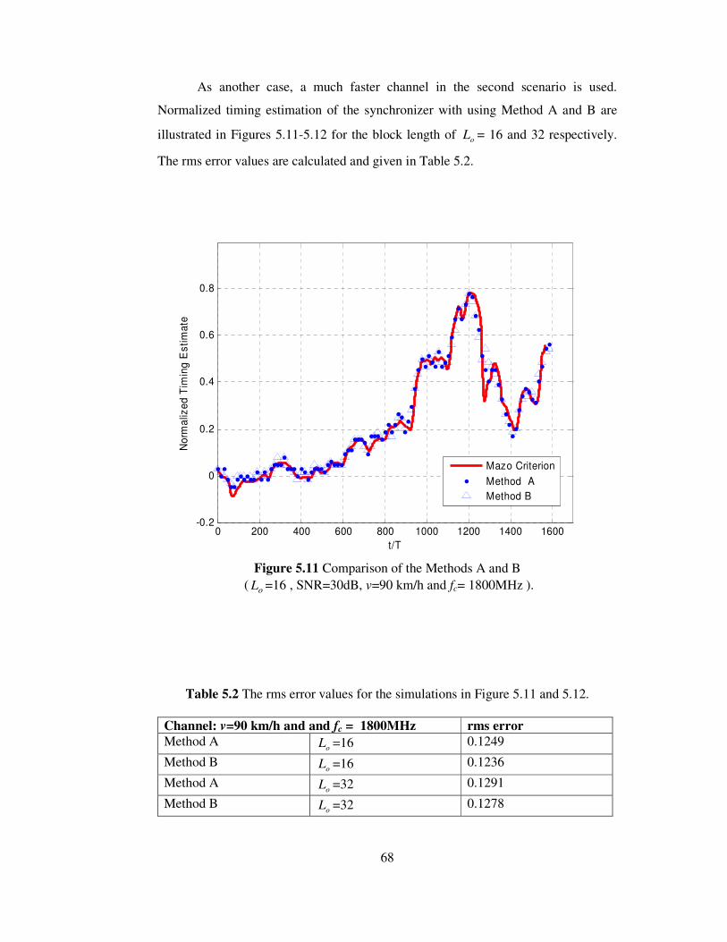
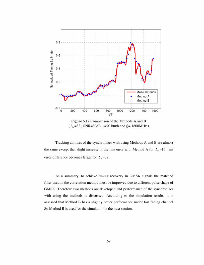
As another case, a much faster channel in the second scenario is used.
Normalized timing estimation of the synchronizer with using Method A and B are
illustrated in Figures 5.11-5.12 for the block length of oL = 16 and 32 respectively.
The rms error values are calculated and given in Table 5.2.
0 200 400 600 800 1000 1200 1400 1600-0.2
0
0.2
0.4
0.6
0.8
t/T
No
rma
lize
d T
imin
g E
sti
ma
te
Mazo Criterion
Method A
Method B
Figure 5.11 Comparison of the Methods A and B
( oL =16 , SNR=30dB, v=90 km/h and fc= 1800MHz ).
Table 5.2 The rms error values for the simulations in Figure 5.11 and 5.12.
Channel: v=90 km/h and and fc = 1800MHz rms error Method A
oL =16 0.1249
Method B oL =16 0.1236
Method A oL =32 0.1291
Method B oL =32 0.1278
69
0 200 400 600 800 1000 1200 1400 1600-0.2
0
0.2
0.4
0.6
0.8
t/T
No
rma
lize
d T
imin
g E
sti
ma
te
Mazo Criterion
Method A
Method B
Figure 5.12 Comparison of the Methods A and B
( oL =32 , SNR=30dB, v=90 km/h and fc= 1800MHz ).
Tracking abilities of the synchronizer with using Methods A and B are almost
the same except that slight increase in the rms error with Method A for oL =16, rms
error difference becomes larger for oL =32.
As a summary, to achieve timing recovery in GMSK signals the matched
filter used in the correlation method must be improved due to different pulse shape of
GMSK. Therefore two methods are developed and performance of the synchronizer
with using the methods is discussed. According to the simulation results, it is
assessed that Method B has a slightly better performance under fast fading channel
So Method B is used for the simulation in the next section.
70
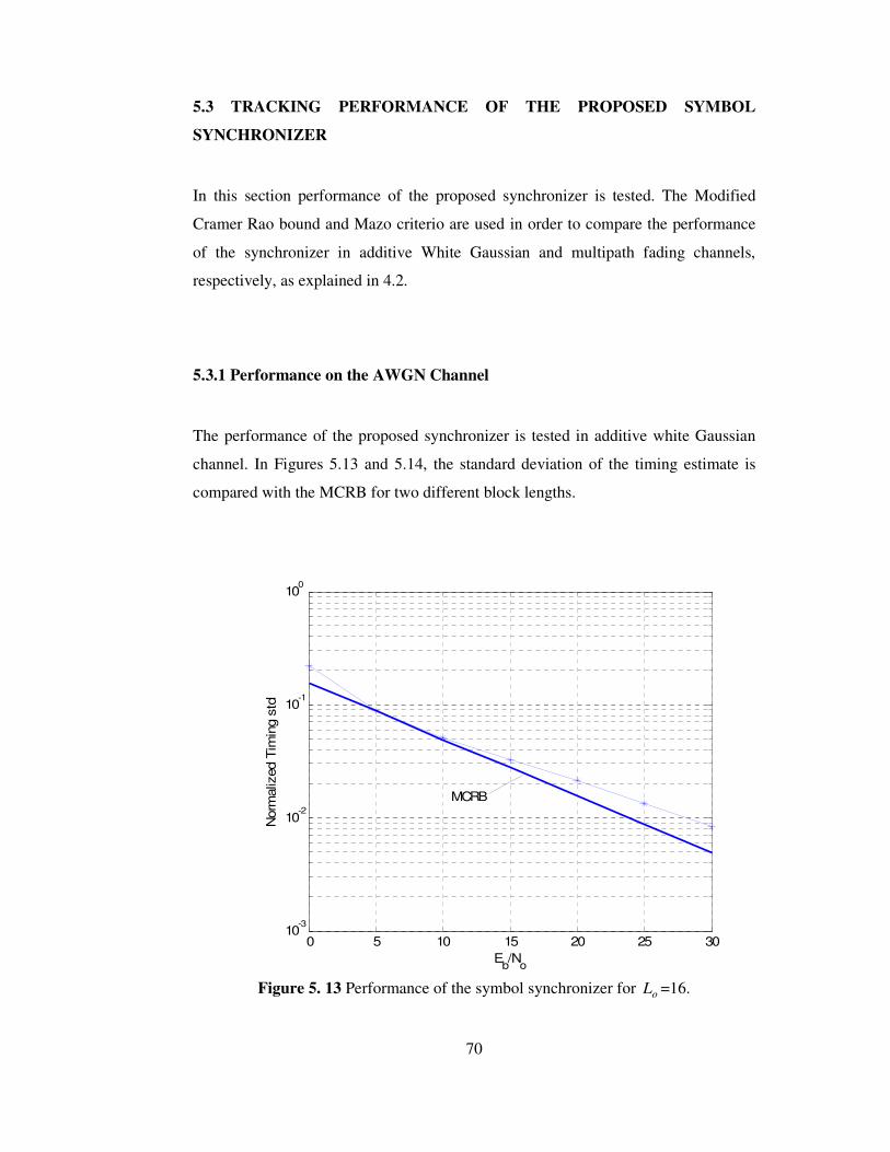
5.3 TRACKING PERFORMANCE OF THE PROPOSED SYMBOL
SYNCHRONIZER
In this section performance of the proposed synchronizer is tested. The Modified
Cramer Rao bound and Mazo criterio are used in order to compare the performance
of the synchronizer in additive White Gaussian and multipath fading channels,
respectively, as explained in 4.2.
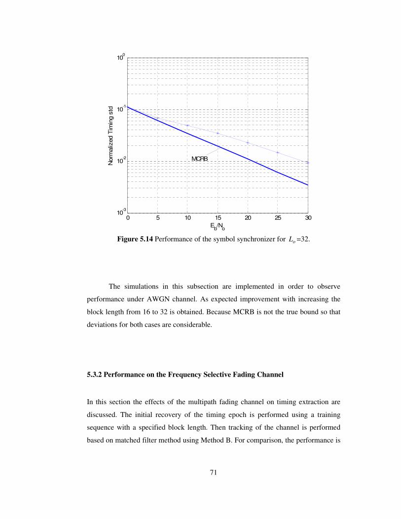
5.3.1 Performance on the AWGN Channel
The performance of the proposed synchronizer is tested in additive white Gaussian
channel. In Figures 5.13 and 5.14, the standard deviation of the timing estimate is
compared with the MCRB for two different block lengths.
0 5 10 15 20 25 3010
-3
10-2
10-1
100
Eb/N
o
Norm
aliz
ed T
imin
g s
td
MCRB
Figure 5. 13 Performance of the symbol synchronizer for oL =16.
71
0 5 10 15 20 25 3010
-3
10-2
10-1
100
Eb/N
o
Norm
aliz
ed T
imin
g s
td
MCRB
Figure 5.14 Performance of the symbol synchronizer for oL =32.
The simulations in this subsection are implemented in order to observe
performance under AWGN channel. As expected improvement with increasing the
block length from 16 to 32 is obtained. Because MCRB is not the true bound so that
deviations for both cases are considerable.
5.3.2 Performance on the Frequency Selective Fading Channel
In this section the effects of the multipath fading channel on timing extraction are
discussed. The initial recovery of the timing epoch is performed using a training
sequence with a specified block length. Then tracking of the channel is performed
based on matched filter method using Method B. For comparison, the performance is
72
given for different values of the parameters; observation interval, SNR and roll of
factor of the interpolation filter.
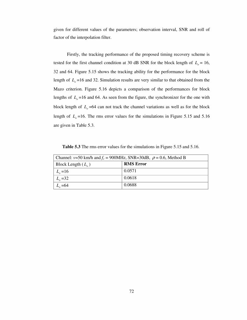
Firstly, the tracking performance of the proposed timing recovery scheme is
tested for the first channel condition at 30 dB SNR for the block length of oL = 16,
32 and 64. Figure 5.15 shows the tracking ability for the performance for the block
length of oL =16 and 32. Simulation results are very similar to that obtained from the
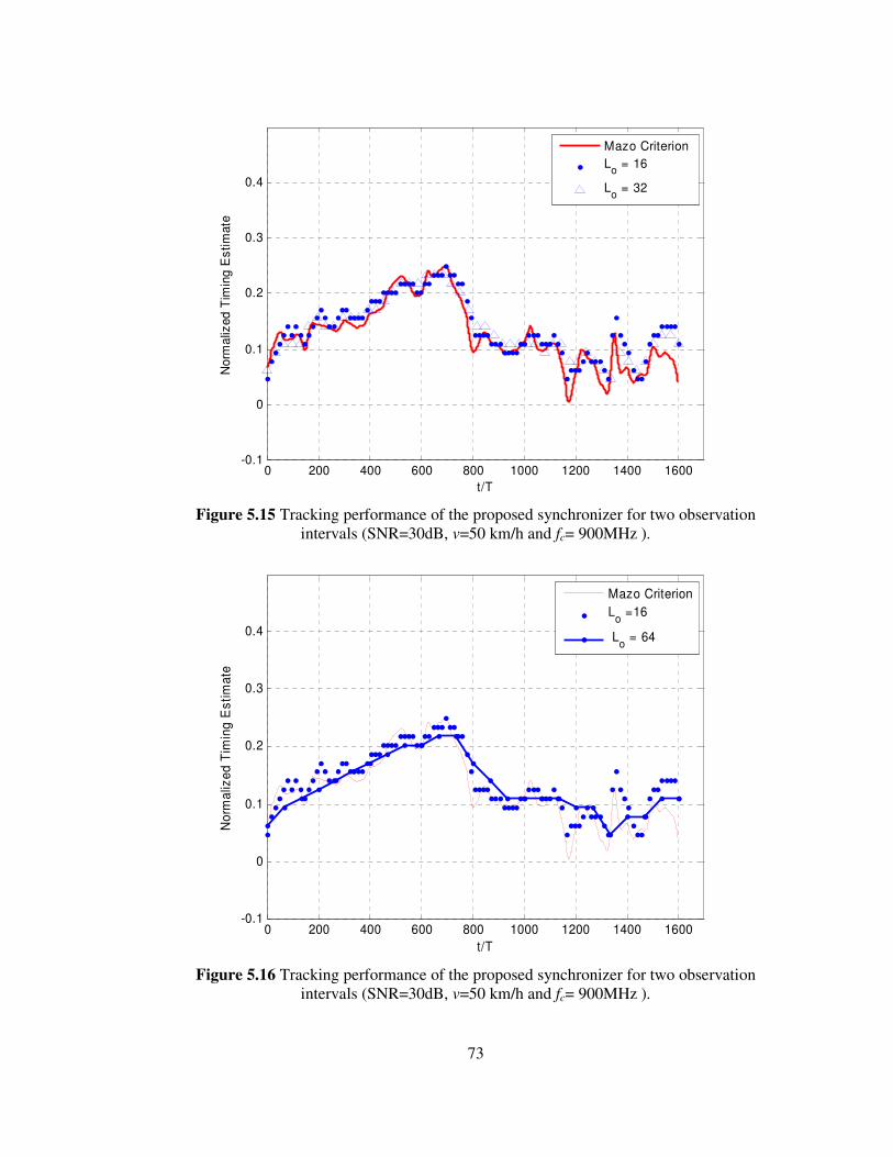
Mazo criterion. Figure 5.16 depicts a comparison of the performances for block
lengths of oL =16 and 64. As seen from the figure, the synchronizer for the one with
block length of oL =64 can not track the channel variations as well as for the block
length of oL =16. The rms error values for the simulations in Figure 5.15 and 5.16
are given in Table 5.3.
Table 5.3 The rms error values for the simulations in Figure 5.15 and 5.16.
Channel: v=50 km/h and fc = 900MHz, SNR=30dB, ρ = 0.6, Method B
Block Length ( oL ) RMS Error
oL =16 0.0571
oL =32 0.0618
oL =64 0.0688
73
0 200 400 600 800 1000 1200 1400 1600-0.1
0
0.1
0.2
0.3
0.4
t/T
No
rma
lized
Tim
ing
Es
tim
ate
Mazo Criterion
Lo = 16
Lo = 32
Figure 5.15 Tracking performance of the proposed synchronizer for two observation
intervals (SNR=30dB, v=50 km/h and fc= 900MHz ).
0 200 400 600 800 1000 1200 1400 1600-0.1
0
0.1
0.2
0.3
0.4
t/T
No
rma
lize
d T
imin
g E
sti
ma
te
Mazo Criterion
Lo =16
Lo = 64
Figure 5.16 Tracking performance of the proposed synchronizer for two observation
intervals (SNR=30dB, v=50 km/h and fc= 900MHz ).
74
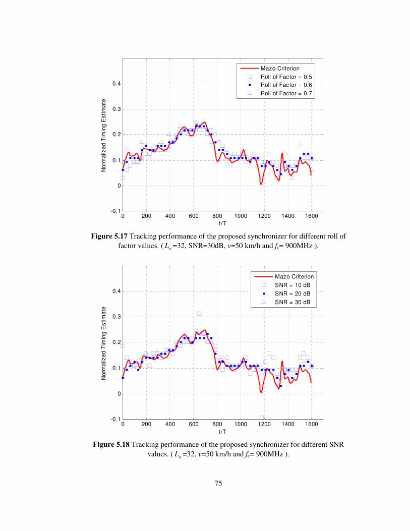
The tracking performance of the proposed timing recovery scheme is tested
for the first channel condition at 30 dB SNR, for the block length of oL =32 for
different roll of factor of the interpolation filter. Figure 5.17 shows the tracking
ability for the performance for 0.5, 0.6 and 0.7 roll of factor of the interpolation
filter. The rms error values for the simulations in Figure 5.17 are given in Table 5.4.
Table 5.4 The rms error values for the simulations in Figure 5.17.
Channel: v=50 km/h and fc = 900MHz, oL =32, Method B
Roll of Factor ( ρ ) rms error
0.5 0.0696 0.6 0.0618 0.7 0.0643
Figure 5.18 shows the tracking performance of the proposed timing recovery
scheme is tested for the first channel condition for block length of oL =32 at 10 dB,
20 dB and 30 dB SNR. The rms error values for the simulations in Figure 5.18 are
given in Table 5.5.As expected, rms error for higher SNR is smaller.
Table 5.5 The rms error values for the simulations in Figure 5.18.
Channel: v=50 km/h and cf = 900MHz, oL =32, ρ =0.6, Method B
SNR rms error 10dB 0.0661 20dB 0.0640 30dB 0.0618
75
0 200 400 600 800 1000 1200 1400 1600-0.1
0
0.1
0.2
0.3
0.4
t/T
No
rma
lized
Tim
ing
Es
tim
ate
Mazo Criterion
Roll of Factor = 0.5
Roll of Factor = 0.6
Roll of Factor = 0.7
Figure 5.17 Tracking performance of the proposed synchronizer for different roll of
factor values. ( oL =32, SNR=30dB, v=50 km/h and fc= 900MHz ).
0 200 400 600 800 1000 1200 1400 1600-0.1
0
0.1
0.2
0.3
0.4
t/T
No
rma
lize
d T
imin
g E
sti
ma
te
Mazo Criterion
SNR = 10 dB
SNR = 20 dB
SNR = 30 dB
Figure 5.18 Tracking performance of the proposed synchronizer for different SNR
values. ( oL =32, v=50 km/h and fc= 900MHz ).
76
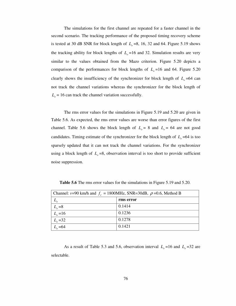
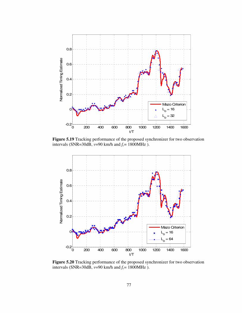
The simulations for the first channel are repeated for a faster channel in the
second scenario. The tracking performance of the proposed timing recovery scheme
is tested at 30 dB SNR for block length of oL =8, 16, 32 and 64. Figure 5.19 shows
the tracking ability for block lengths of oL =16 and 32. Simulation results are very
similar to the values obtained from the Mazo criterion. Figure 5.20 depicts a
comparison of the performances for block lengths of oL =16 and 64. Figure 5.20
clearly shows the insufficiency of the synchronizer for block length of oL =64 can
not track the channel variations whereas the synchronizer for the block length of
oL = 16 can track the channel variation successfully.
The rms error values for the simulations in Figure 5.19 and 5.20 are given in
Table 5.6. As expected, the rms error values are worse than error figures of the first
channel. Table 5.6 shows the block length of oL = 8 and
oL = 64 are not good
candidates. Timing estimate of the synchronizer for the block length of oL =64 is too
sparsely updated that it can not track the channel variations. For the synchronizer
using a block length of oL =8, observation interval is too short to provide sufficient
noise suppression.
Table 5.6 The rms error values for the simulations in Figure 5.19 and 5.20.
Channel: v=90 km/h and cf = 1800MHz, SNR=30dB, ρ =0.6, Method B
oL rms error
oL =8 0.1414
oL =16 0.1236
oL =32 0.1278
oL =64 0.1421
As a result of Table 5.3 and 5.6, observation interval oL =16 and oL =32 are
selectable.
77
0 200 400 600 800 1000 1200 1400 1600-0.2
0
0.2
0.4
0.6
0.8
t/T
Norm
aliz
ed T
imin
g E
stim
ate
Mazo Criterion
Lo = 16
Lo = 32
Figure 5.19 Tracking performance of the proposed synchronizer for two observation intervals (SNR=30dB, v=90 km/h and fc= 1800MHz ).
0 200 400 600 800 1000 1200 1400 1600-0.2
0
0.2
0.4
0.6
0.8
t/T
Norm
aliz
ed T
imin
g E
stim
ate
Mazo Criterion
Lo = 16
Lo = 64
Figure 5.20 Tracking performance of the proposed synchronizer for two observation intervals (SNR=30dB, v=90 km/h and fc= 1800MHz ).
78
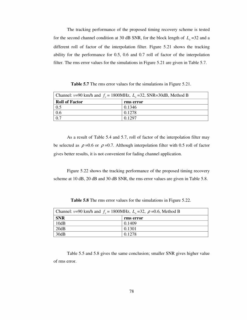
The tracking performance of the proposed timing recovery scheme is tested
for the second channel condition at 30 dB SNR, for the block length of oL =32 and a
different roll of factor of the interpolation filter. Figure 5.21 shows the tracking
ability for the performance for 0.5, 0.6 and 0.7 roll of factor of the interpolation
filter. The rms error values for the simulations in Figure 5.21 are given in Table 5.7.
Table 5.7 The rms error values for the simulations in Figure 5.21.
Channel: v=90 km/h and cf = 1800MHz, oL =32, SNR=30dB, Method B
Roll of Factor rms error 0.5 0.1346 0.6 0.1278 0.7 0.1297
As a result of Table 5.4 and 5.7, roll of factor of the interpolation filter may
be selected as ρ =0.6 or ρ =0.7. Although interpolation filter with 0.5 roll of factor
gives better results, it is not convenient for fading channel application.
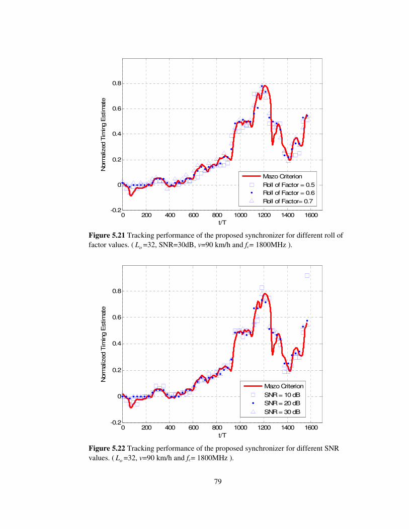
Figure 5.22 shows the tracking performance of the proposed timing recovery
scheme at 10 dB, 20 dB and 30 dB SNR, the rms error values are given in Table 5.8.
Table 5.8 The rms error values for the simulations in Figure 5.22.
Channel: v=90 km/h and cf = 1800MHz, oL =32, ρ =0.6, Method B
SNR rms error 10dB 0.1409 20dB 0.1301 30dB 0.1278
Table 5.5 and 5.8 gives the same conclusion; smaller SNR gives higher value
of rms error.
79
0 200 400 600 800 1000 1200 1400 1600-0.2
0
0.2
0.4
0.6
0.8
t/T
Norm
aliz
ed T
imin
g E
stim
ate
Mazo Criterion
Roll of Factor = 0.5
Roll of Factor = 0.6
Roll of Factor= 0.7
Figure 5.21 Tracking performance of the proposed synchronizer for different roll of factor values. ( oL =32, SNR=30dB, v=90 km/h and fc= 1800MHz ).
0 200 400 600 800 1000 1200 1400 1600-0.2
0
0.2
0.4
0.6
0.8
t/T
Norm
aliz
ed T
imin
g E
stim
ate
Mazo Criterion
SNR = 10 dB
SNR = 20 dB
SNR = 30 dB
Figure 5.22 Tracking performance of the proposed synchronizer for different SNR values. ( oL =32, v=90 km/h and fc= 1800MHz ).
80
CHAPTER 6
CONCLUSION
Throughout this study, it has been noticed that although there are plenty of research
studies on the area of symbol synchronization for CPM signals, there are still issues
that are to be investigated in the frequency selective fading channel transmission
area.
In this study, symbol timing recovery for CPM signals over multipath fading
channel was examined by employing GMSK signal. The reason of choosing GMSK
among the CPM family is its common use within digital communication systems like
GSM and DECT.
In the GSM system, specific training sequences which have good
crosscorrelation properties are used for channel identification. In this study, the
channel identification solution based on correlation method was reviewed and the
training sequences were presented. In order to take advantage of the good correlation
property, the training sequences were used throughout the initial timing acquisition
in simulations.
As it is mentioned in the literature, approximation of GMSK modulation as a
linear modulation is necessary to enable the use of MLSE method in receiver.
Consequently, the linearly approximated GMSK was reviewed, power spectrum
density and waveform envelope of the linear GMSK signal were examined and
81
observed as expected. Time varying multipath fading channel with TU delay power
profile has been simulated.
The performance of the recovery scheme in MSK over multipath fading
channel was examined in [1] by using the proposed timing recovery scheme which
was based on correlation (matched filter) method by using the samples of the
received signal. The same matched filter could not be used for both MSK and GMSK
modulation scheme due to different spanning duration of their pulse shapes. As a
result, two methods; “Method A” and “Method B” were developed in order to
construct the matched filter for the application on GMSK signals.
Tracking ability of the synchronizer by using both methods was simulated. In
order to compare these methods rms error values were calculated by using Mazo
criterion which is an important tool in the context. According to the simulation
figures, it was observed that both methods could track channel variation successfully.
However, it was assessed that Method B has a slightly better performance than
Method A especially under fast fading channel conditions with respect to rms error
values. Consequently, Method B was used for the simulations throughout the study.
Precise timing estimation was achieved by employing interpolation and
iterative maximum search process. Moreover, interpolation filter structure was
examined with simulations. The initial timing information was acquired by using a
training sequence, placed in front of the data burst. Tracking mode is performed by
tentative decisions from MLSE receiver in the proposed timing recovery [1].
However, in this study, tentative decisions were assumed to be error free and
tracking mode was performed by them. Furthermore, Mazo criterion was used as a
basis for the tracking performance of the proposed scheme.
Simulations were repeated for different value of parameters; length of
observation interval, roll of factor of interpolation filter and SNR. By investigating
82
the effects of the parameters on the performance of the synchronizer, sensitivity
analyses were performed.
As a future work, tentative decisions may be acquired from the MLSE receiver
by using Viterbi Algorithm. The performance of the MLSE receiver depends on the
available estimate of the channel impulse response. Therefore, channel estimation
techniques (blind or non blind) may be investigated. Thus, the performance of the
synchronizer may be tested in a more complex receiver model.
83
REFERENCES
[1] S. Sezginer, “Symbol Synchronization For MSK Signals Based On Matched Filtering,” M.Sc. Thesis, Electrical and Electronics Eng. Dept., Middle East Technical University, Ankara, September 2003.
[2] S. Sezginer, Y. Tanık, “An Improved Matched Filter Based Symbol Synchronizer For MSK Transmission Over Fading Multipath Channels,” IEEE Vehicular Technology Conference, vol. 3, pp. 1678 – 1682, Sept. 2004.
[3] J. G Proakis, “Digital Communications,” Singapore, McGraw-Hill, 1995.
[4] S. Eken, “A Study on GMSK Modulation And Channel Simulation,” M.Sc. Thesis, Electrical and Electronics Eng. Dept., Middle East Technical University, Ankara, Feb. 1994.
[5] M. C. Jeruchim, P. Balaban and K. S. Shanmugan, “Simulation of Communication Systems Modeling, Methodology, and Techniques,” New York, Second Ed., Kluwer Academic, 2002.
[6] J. Eberspacher, H-J Vögel, C. Bettstetter, “GSM Switching, Services and Protocols,” John-Wiley, Second Edition, 1999.
[7] P. A. Laurent, “Exact and Approximate Construction of Digital Phas Modulation by Superposition of Amplitude Modulated Pulses (AMP),” IEEE Trans. Commun., vol. Com-34, pp. 150-160, Feb. 1986.
[8] P. Jung, “Laurent’s representation of binary digital continuous phase modulated signals with modulation index 1/2 revisited,” IEEE Trans. Commun., vol. 42, pp. 221-224, 1994.
84
[9] A Wiesler, F. K. Jondral, “A software Radio For Second and Third Generation Mobile Systems ”, IEEE Trans. Commun., vol. Com-51, No 4, pp 738- 748 July 2002.
[10] A Wiesler, R. Machauer, F. Jondral, “Comparison of GMSK and Linear Approximated GMSK For Use In Software Radio”, IEEE, pp 557-560, 1998.
[11] B. Canpolat, “Design and Simulation of an Adaptive MLSE Receiver for GSM System,” M.Sc. Thesis, Electrical and Electronics Eng. Dept., Middle East Technical University, Ankara, Feb. 1994.
[12] A. Mehrotra, GSM System Engineering, Boston, Artech House, 1996.
[13] H. Meyr and G. Ascheid, Synchronization in Digital Communications, vol.1, New York: John Wiley & Sons, 1990.
[14] H. Meyr, M Moeneclaey, and S. A. Fechtel, Digital Communication, New York: McGraw-Hill, 1968.
[15] U. Mengali and A. N. D’Andrea, Synchronization Techniques for Digital Receivers, New York: Plenum Press, 1997.
[16] R. de Buda, ”Coherent Demodulation of Frequency Shift Keying with Low Deviation Ratio,” IEEE Trans. Commun., vol. COM-20, pp. 429-435, June 1972.
[17] T. Aulin and C. E. Sundberg, “Synchronization Properties of Continuous Phase Modulation,” in Proc. Int Conf. Commun., Philadelphia, PA, pp. D7.1.1-D7.1.7, June 1982.
[18] A. N. D’Andrea, U. Mengali, and R. Reggiannini, “Carrier Phase and Clock Recovery for Continuous Phase Modulated Signals,” IEEE Trans. Commun., vol. COM-35, pp. 1095-1101, Oct. 1987.
[19] J. Huber and W. Liu, “Data-Aided Synchronization of Coherent CPM Receivers,” IEEE Trans. Commun., vol. COM-40 pp. 178-189, Jan. 1992.
[20] R. Melhan, Y.E. Chen, and H. Meyr, “A Fully Digital Feedforward MSK Demodulator with Joint Frequency Offset and Symbol Timing Estimation for
85
Burst Mode Mobile Radio”, IEEE Trans. Veh. Techol., vol. VT-42 pp. 434-443, Nov. 1993.
[21] U. Lambrette and H. Meyr, “Two Timing Recovery Algorithms for MSK,” in Proc.ICC’94, New Orleans, LO, pp. 918-992, May 1994.
[22] M. Morelli and G. M. Vitetta, “Two Timing Recovery Algorithms for MSK,” in Proc. ICC’94, New Orleans, LO, pp. 1997-1999, Dec. 2000.
[23] F. Patenaude, J. H. Lodge, and P. A. Galko, “Symbol Timing Tracking for Continuous Phase Modulation over Fast Flat-Fading Channels,” IEEE Trans. Veh. Technol., vol. VT-40 pp. 615-626, Aug. 1991.
[24] L.E. Franks, “Carrier and Bit Synchronization in Data Communication- A Tutorial Review,” IEEE Trans. Commun., vol. COM-28, pp. 1107-1120, Aug. 1980.
[25] L. P. Sabel, “Maximum Likelihood Approach to Symbol Timing Recovery in Digital Communications,” Ph.D. Thesis, Sch. Of Elec. Eng. Univ. South Australia, South Australia, Oct. 1993.
[26] H.L. Van Trees, Detection, Estimation and Modulation Theory Part I, New York: John Wiley & Sons, 1968.
[27] K. H. Muller and M. Muller, “Timing Recovery in Digital synchronous Data Receivers,” IEEE Trans. Commun., vol. COM-24, pp. 516-531, May 1976.
[28] J. E. Mazo, “Optimum Timing Phase for an Infinite Equalizer,” Bell Syst, Tech. J., vol. 54, pp. 189-201, 1975.
[29] R. W. Lucky, J. Salz, and E. J. Weldon, Jr., Principals of Data Communication, New York: McGraw-Hill, 1968.
[30] A. V. Oppenheim and R. W: Schafer, Discrete-Time Signal Processing, Upper Saddle River, NJ: Prentice-Hall, 1999.
[31] A. N. D’Andrea, U. Mengali, and M. Morelli, “Symbol Timing Estimation with CPM Modulation,” IEEE Trans. Commun., vol. COM-44, pp. 1362-1372, Oct. 1996.
86
[32] R. Steele, Chin-Chun Lee, P. Gould, GSM, cdmaOne and 3G Systems, West Sussex, John Wiley & Sons ltd., 2001.
87
APPENDIX A
CPM SIGNALS
Continuous phase modulation (CPM) conserves and reduces signal energy and
bandwidth at the same time. CPM is a constant envelope, nonlinear modulation
method with memory. The constant envelope property of CPM schemes makes
possible to use non-linear amplifiers. The phase is a continuous function of time
since the data symbols modulate the instantaneous phase of the transmitted signal.
A.1 SIGNAL MODEL
The complex envelope of a CPM signal is given by [31]
));((2)( ταφθ −+= tis e
T
Ets , (A.1)
where Es is the energy per signaling interval, T is the symbol period, θ is carrier
phase, τ is timing epoch, α ={ α i } are data sequence from the alphabet {±1, ±3,…..,
±(M-1)} and φ (α,t) is the information-bearing phase:
88
∑ −=i
ii itqht )(2);( ταπαφ . (A.2)
The parameter hi is called the modulation index.. When hi =h for all i, the
modulation index is fixed for all symbols. When the modulation index varies from
one symbol to another, the CPM signal is called multi-h. q(t) is the phase pulse of the
modulator, which is related to the frequency pulse g(t) by
∫∞−
=t
dgtq ττ )()( , (A.3)
and is normalized in such a way that
1/ 2, t( )
0 , t<0
LTq t
≥=
. (A.4)
The phase pulse is nonzero in the interval t ∈ (0, LT), where L is an integer
called the correlation length. If L=1, the modulated signal is called full response
CPM. If L>1, the modulated signal is called partial response CPM. The CPM signal
has memory that is introduced through the phase continuity. For L>1, additional
memory is introduced in the CPM signal by the pulse g(t).
By choosing different frequency pulses and varying the parameters h and M,
a great variety of CPM schemes may be formed.
A.2 MINIMUM SHIFT KEYING AND GAUSSIAN MINIMUM SHIFT
KEYING
A subset of CPM signals is minimum shift keying (MSK) corresponds to
h=1/2, M=2 and a rectangular frequency pulse
89
1/ 2 , 0< t( )
0 , elsewhere
T Tg t
≤=
. (A.5)
MSK modulation is a constant envelope digital modulation. The spectrum of
MSK is quite large and substantial energy exists in the sidelobes.
The spectrum of an MSK modulated signal may be compressed by filtering
the modulating baseband pulses to produce much smoother changes in frequency,
thereby compressing the bandwidth of the modulated signal. The type of filter used
has a Gaussian impulse response and the resulting modulation scheme is called
Gaussian MSK (GMSK). The relative bandwidth of the Gaussian filter defines the
spectrum compression that is achieved, i.e. a smaller filter bandwidth results in a
narrower modulated spectrum. Unfortunately, the Gaussian filter also introduces ISI
whereby each modulation symbol spreads into adjacent symbols [32].
In this thesis, the emphasis is given on Gaussian MSK (GMSK), which is
used as the GSM modulation scheme. GMSK is obtained by letting h=1/2, M=2 and
g(t) is given by,
g(t)=h(t)* rect(t/T). (A.6)
Gaussian shaped impulse response, h(t) is given by;
2
2 2
1( ) exp
22
th t
TT σπσ
= −
, (A.7)
where
ln 2 / 2 BTσ π= (A.8)
90
here, B is the 3 dB bandwidth of the filter.
rect (t/T) is defined by;
1/ , t / 2( / )
0 , otherwise
T Trect t T
<=
, (A.9)
then,
1 2 ( / 2) 2 ( / 2)( )
2 ln 2 ln 2
B t T B t Tg t erf erf
T
π π − += − + −
, (A.10)
where
2
0
2( ) exp( )
x
erf x dυ υπ
= −∫ (A.11)
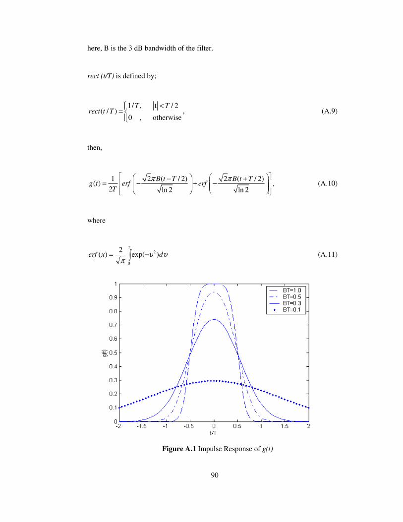
Figure A.1 Impulse Response of g(t)
91
The resulting impulse response g(t) is given in Fig A.1 for some values of
BT. Notice that with decreasing BT the impulse response becomes broader. For
BT → ∞ it converges to rect(.) function, also GMSK signal converges to MSK
signal. The Gaussian low-pass filtering has the effect of additional smoothing but
also of the broadening the impulse response g(t). This means that, the power
spectrum of the signal is made narrower, but on the other hand the individual impulse
responses are “smeared” across several bit durations, which leads to increase
intersymbol interference.
92
APPENDIX B
APPROXIMATION OF GMSK TO LINEAR QAM SIGNAL
The GMSK signal can be approximated to a linear QAM signal by adopting a
suitable pulse shape [4]. The pulse shape happens to be an approximately Gaussian
function spanning a time interval of approximately four symbol durations as will be
derived in this appendix.
The phase expression of GMSK signal is given as;
∑∫ −=∞− k
k
t
dkTgat ττπ
φ )(2
)( , (B.1)
which can also be expressed as;
∫∑−
∞−
=kTt
k
k dgat ττπ
φ )(2
)( , (B.2)
where ak’s are the differentially encoded bits in the form of ± 1, and g(t) is the
shaping function given as;
93
++
−−= )
2ln
)2(2()
2ln
)2(2(
2
1)(
TtBerf
TtBerf
Ttg
ππ. (B.3)
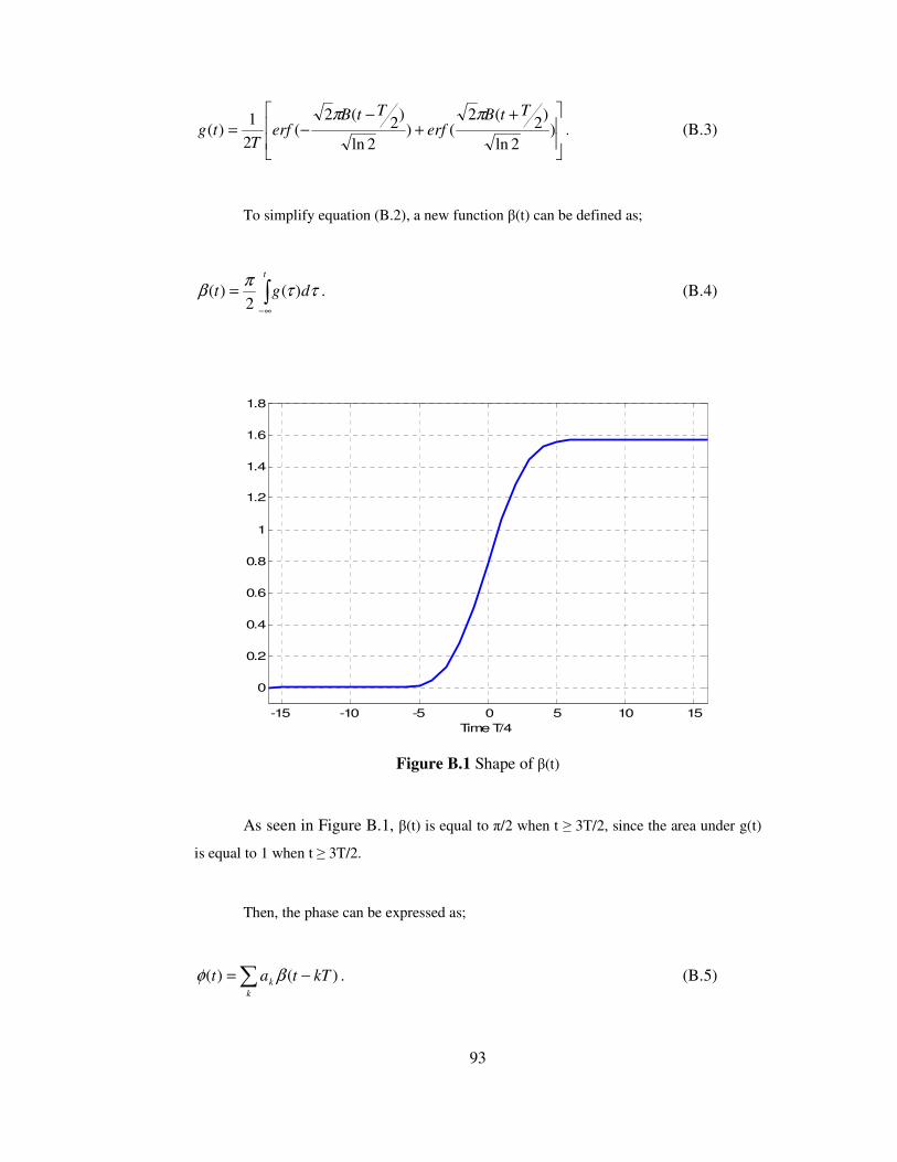
To simplify equation (B.2), a new function β(t) can be defined as;
∫∞−
=t
dgt ττπ
β )(2
)( . (B.4)
-15 -10 -5 0 5 10 15
0
0.2
0.4
0.6
0.8
1
1.2
1.4
1.6
1.8
Time T/4
Figure B.1 Shape of β(t)
As seen in Figure B.1, β(t) is equal to π/2 when t ≥ 3T/2, since the area under g(t)
is equal to 1 when t ≥ 3T/2.
Then, the phase can be expressed as;
)()( kTtatk
k −=∑ βφ . (B.5)
94
Thus, the baseband GMSK signal can be rewritten as;
sb(t)=exp j
−∑
k
k kTta )(β , (B.6)
Now consider the time interval (2n-1)T/2 ≤ t ≤ (2n+1)T/2. For this interval, if
k ≤ (n-2) then β(t-kT)= π/2 since in this case (t-kT) ≥ 3T/2. Therefore, the above equation
can be rewritten as;
sb(t)=exp j
−+− ∑∑
+
−=
−
−∞=
1
1
2
)()(n
nk
k
n
k
k kTtakTta ββ , (B.7)
and for the time interval (2n-1)T/2 ≤ t ≤ (2n+1)T/2 one can get;
sb(t)=exp j
∑
−
=
2
02
n
k
kaπ
exp j
−∑
+
−=
1
1
)(n
nk
k kTta β , (B.8)
sb(t)=exp j
∑
−
=
2
02
n
k
kaπ
[ ]1
1
exp j ( ( ) )n k
k
a t n k Tβ−=−
− −∏ , (B.9)
In the light of above equations, it can be shown that [4] the baseband GMSK
signal may be expressed as;
sb(t)=3 2
0 1
exp ( )2
N
n N i ki k
N k n i
j a a C t NTπ
α∞
−=−∞ = =−∞ =
− −
∑ ∑ ∑ ∑ , (B.10)
where,
001 =α 111 =α 021 =α 131 =α
95
002 =α 012 =α 122 =α 132 =α
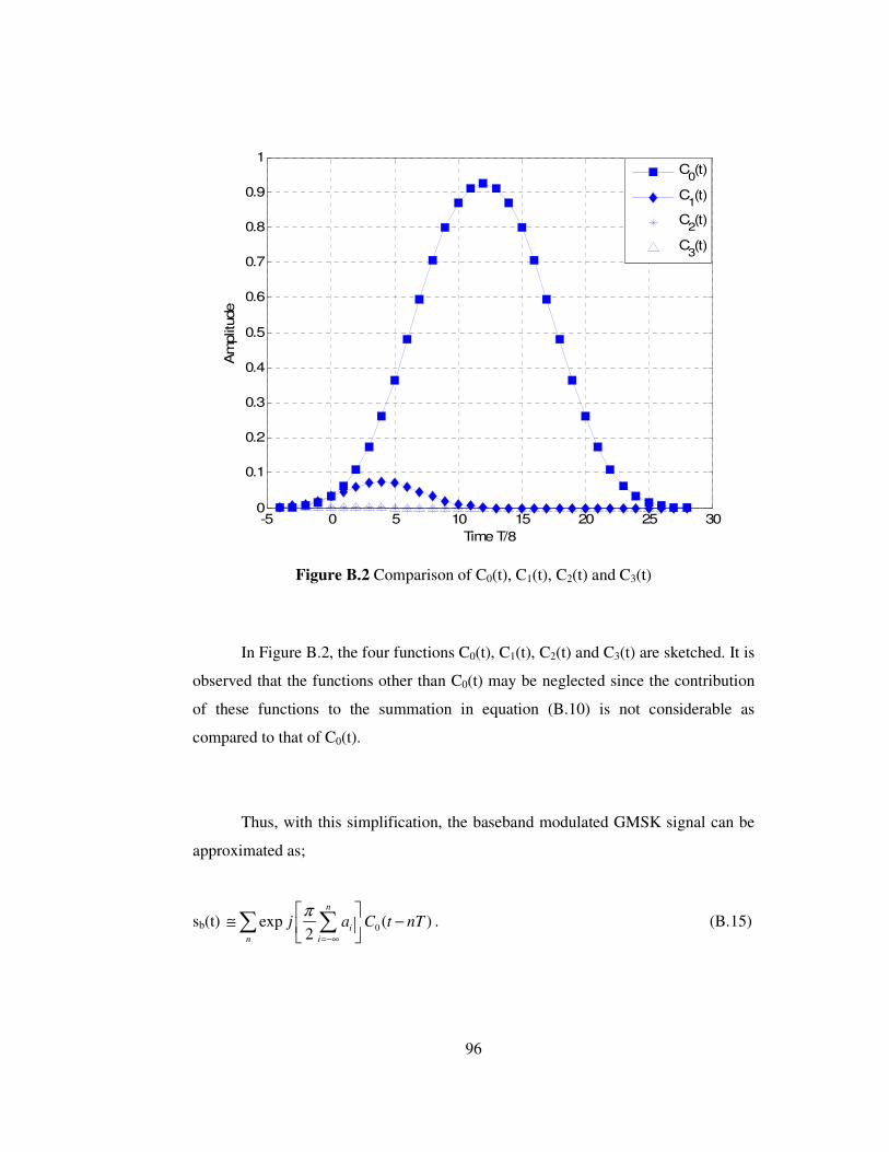
and the functions Ck(t), k=0,1,2,3 are defined by;