SYMBOLIC ALGORITHMS AND SOFTWARE FOR THE

PAINLEVE TEST AND RECURSION OPERATORS FOR

NONLINEAR PARTIAL DIFFERENTIAL EQUATIONS

by

Douglas E. Baldwin

Copyright 2004 by Douglas E. Baldwin

All Rights Reserved

Dr. Graeme Fairweather

Professor and Head

Department of Mathematical

and Computer Sciences

Approved:

Dr. Willy Hereman

Thesis Advisor

Signed:

Douglas E. Baldwin

Golden, Colorado

Date

Golden, Colorado

Date

A thesis submitted to the Faculty and Board of Trustees of the Colorado School

of Mines in partial fulfillment of the requirements for the degree of Master of Science

(Mathematical and Computer Sciences).

ii

ABSTRACT

This thesis discusses two algorithms for studying the complete integrability of polyno-

mial nonlinear differential equations. The first algorithm is the well known Painleve

test, which analyzes the singularity structure of the solutions of ordinary and partial

differential equations. The absence of certain types of singularities (e.g., movable

branch points) is a strong indicator that the differential equation is completely in-

tegrable. We have fully automated this notoriously tedious algorithm as the Mathe-

matica package PainleveTest.m.

The second is an algorithm for computing and testing recursion operators of (1+1)-

dimensional evolution equations. A recursion operator links the generalized symme-

tries of an equation. Therefore, the recursion operator is an important tool in proving

the existence of infinitely many generalized symmetries, a strong indicator of com-

plete integrability. While finding the form of the operator requires a certain amount

of inspired guesswork, testing the operator is fairly straightforward albeit inordinately

tedious. Therefore, we have completely automated both the tasks of finding the oper-

ator and testing the operator as the Mathematica package PDERecursionOperator.m.

Completely integrable differential equations model such physically interesting phe-

nomena as reaction-diffusion systems, population and molecular dynamics, nonlinear

networks, chemical reactions, and material science (in particular solid mechanics and

elastic materials). The two primary methods for solving a completely integrable non-

linear evolution equation are by explicit transformations into a linear equation or by

using the inverse scattering transform. The inverse scattering transform is a non-

trivial exercise in analysis with no systematic way to determine a priori if it will

be successful. However, passing the Painleve test or having a recursion operator is

a strong indicator that the differential equation will be solvable using the inverse

scattering transformation.

iii

TABLE OF CONTENTS

ABSTRACT . . . . . . . . . . . . . . . . . . . . . . . . . . . . . . . . . . . . . . . . . . . . . . . . . . . . . . . . iii

ACKNOWLEDGEMENTS . . . . . . . . . . . . . . . . . . . . . . . . . . . . . . . . . . . . . . . . . . vi

1 INTRODUCTION AND HISTORY . . . . . . . . . . . . . . . . . . . . . . . . . . . . . . 1

1.1 Motivation . . . . . . . . . . . . . . . . . . . . . . . . . . . . . . . . . 1

1.2 History and Purpose of Painleve Analysis . . . . . . . . . . . . . . . . 2

1.3 History and Purpose of Recursion Operators . . . . . . . . . . . . . . 4

2 THE PAINLEVE TEST . . . . . . . . . . . . . . . . . . . . . . . . . . . . . . . . . . . . . . . . . . 9

2.1 Introduction . . . . . . . . . . . . . . . . . . . . . . . . . . . . . . . . 9

2.2 Algorithm . . . . . . . . . . . . . . . . . . . . . . . . . . . . . . . . . 10

2.3 Examples . . . . . . . . . . . . . . . . . . . . . . . . . . . . . . . . . 14

2.3.1 Painleve equation I . . . . . . . . . . . . . . . . . . . . . . . . 14

2.3.2 Korteweg-de Vries equation . . . . . . . . . . . . . . . . . . . 15

2.3.3 A system of ODEs . . . . . . . . . . . . . . . . . . . . . . . . 17

2.3.4 Hirota-Satsuma system . . . . . . . . . . . . . . . . . . . . . . 20

2.4 Implementation . . . . . . . . . . . . . . . . . . . . . . . . . . . . . . 23

2.4.1 Algorithm to determine the dominant behavior . . . . . . . . 23

2.4.2 Algorithm to determine the resonances . . . . . . . . . . . . . 26

2.4.3 Algorithm to determine the constants of integration . . . . . . 28

2.5 Other Software Packages . . . . . . . . . . . . . . . . . . . . . . . . . 29

2.6 Additional Examples . . . . . . . . . . . . . . . . . . . . . . . . . . . 29

2.6.1 Boussinesq equation . . . . . . . . . . . . . . . . . . . . . . . 29

2.6.2 Clarkson equation . . . . . . . . . . . . . . . . . . . . . . . . . 30

2.6.3 Sine-Gordon and Liouville equations . . . . . . . . . . . . . . 30

2.6.4 Generalized nonlinear Schrodinger equation . . . . . . . . . . 32

2.6.5 Fifth-order generalized Korteweg-de Vries equation . . . . . . 33

iv

3 RECURSION OPERATORS . . . . . . . . . . . . . . . . . . . . . . . . . . . . . . . . . . . . . 35

3.1 Introduction . . . . . . . . . . . . . . . . . . . . . . . . . . . . . . . . 35

3.2 Integro-differential Operators . . . . . . . . . . . . . . . . . . . . . . 36

3.3 Scaling Invariance, Conserved Densities and Generalized Symmetries 37

3.3.1 Scaling invariance . . . . . . . . . . . . . . . . . . . . . . . . . 37

3.3.2 Conservation laws and generalized symmetries . . . . . . . . . 38

3.4 Algorithm for Computing Recursion Operators . . . . . . . . . . . . . 41

3.5 Examples . . . . . . . . . . . . . . . . . . . . . . . . . . . . . . . . . 42

3.5.1 Korteweg-de Vries equation . . . . . . . . . . . . . . . . . . . 42

3.5.2 Kaup-Kupershmidt equation . . . . . . . . . . . . . . . . . . . 43

3.5.3 Hirota-Satsuma system . . . . . . . . . . . . . . . . . . . . . . 45

3.6 Implementation . . . . . . . . . . . . . . . . . . . . . . . . . . . . . . 47

3.6.1 Algorithm for building the candidate recursion operator . . . . 48

3.6.2 Algorithm for determining the unknown coefficients . . . . . . 50

3.7 Other Software Packages . . . . . . . . . . . . . . . . . . . . . . . . . 54

3.8 Additional Examples . . . . . . . . . . . . . . . . . . . . . . . . . . . 55

3.8.1 Nonlinear Schrodinger equation . . . . . . . . . . . . . . . . . 55

3.8.2 Burgers’ equation . . . . . . . . . . . . . . . . . . . . . . . . . 56

3.8.3 Drinfel’d-Sokolov-Wilson equation . . . . . . . . . . . . . . . . 57

4 CONCLUSION AND FUTURE WORK . . . . . . . . . . . . . . . . . . . . . . . . . . 60

LIST OF ABBREVIATIONS . . . . . . . . . . . . . . . . . . . . . . . . . . . . . . . . . . . . . . . . 62

REFERENCES CITED . . . . . . . . . . . . . . . . . . . . . . . . . . . . . . . . . . . . . . . . . . . . . 63

v

ACKNOWLEDGEMENTS

I greatly appreciate the help of Dr. Willy Hereman; working closely with him over

the last five years has transformed me from a tyro freshman into the researcher I am

today.

Without the support of the National Science Foundation Research Award CCR-

9901929, this research would not have been possible.

Many thanks go to my thesis committee members, Dr. Paul Martin and Dr. John

DeSanto for their helpful comments and suggestions.

Above all, I would like to thank my parents for their limitless love, encouragement

and praise.

vi

1

CHAPTER 1

INTRODUCTION AND HISTORY

1.1 Motivation

There was a revolution in nonlinear physics in the latter part of the twentieth century;

the discovery of solitons and strange attractors radically changed the way scientists

and mathematicians view nonlinearity [34]. While strange attractors and chaos the-

ory give us a better understanding of the erratic and often unpredictable nature of

natural phenomena, soliton theory helps explain natural phenomena that are sur-

prisingly predictable and regular even under conditions that would normally destroy

such properties. A soliton is a solitary wave which preserves its shape and velocity

after nonlinearly interacting with other solitary waves or (arbitrary) localized distur-

bances. The study of solitons leads to the concept of complete integrability and the

construction of solutions to a wide class of nonlinear differential equations [1].

Completely integrable nonlinear partial differential equations (PDEs) often have

remarkable properties, such as infinitely many generalized symmetries, infinitely many

conservation laws, the Painleve property (perhaps after a change of variables), Back-

lund and Darboux transformations, a bilinear form, and a Lax pair (cf. [2, 14, 29, 30]).

These remarkable differential equations model such physically interesting phenom-

ena as reaction-diffusion systems, population and molecular dynamics, nonlinear net-

works, chemical reactions, and material science (in particular solid mechanics and

elastic materials). By investigating the complete integrability of nonlinear PDEs, we

can gain important insight into the nature of their solutions.

There are numerous methods for solving completely integrable nonlinear PDEs,

for instance by explicit transformations into linear equations or by using the inverse

scattering transform (IST) [14]. Recently, progress has been made using Math-

ematica and Maple in applying the IST-method to compute solutions for difficult

equations, including the complicated Camassa-Holm equation [28]. While there is as

yet no systematic way to determine if a differential equation is solvable using the IST-

2

method [32], the possession of infinitely many generalized symmetries, the Painleve

property, etc. are strong indicators that it will be.

In this thesis, we discuss two algorithms and their implementations [4, 5] which

may greatly aid the investigation of complete integrability. In Chapter 2 we present

the well known algorithm for the Painleve test, which analyzes the singularity struc-

ture of the solutions of ordinary and partial differential equations. The absence of

certain types of singularities (e.g., movable branch points) is a strong indicator that

the differential equation is completely integrable. We have fully automated this no-

toriously tedious algorithm as the Mathematica package PainleveTest.m [4].

In Chapter 3 we give an algorithm for computing and testing recursion oper-

ators [23, 36] of (1 + 1)-dimensional polynomial evolution equations. A recursion

operator links the generalized symmetries of an equation. Therefore, the recursion

operator is an important tool in proving the existence of infinitely many general-

ized symmetries. Fokas [14] considers generalized symmetries as the basic feature

of completely integrable equations, and gives the existence of an infinite number of

generalized symmetries as a definition of complete integrability. While finding the

form of the operator requires a certain amount of inspired guesswork, testing the op-

erator is fairly straightforward albeit inordinately tedious. Thus, we have completely

automated both the tasks of finding the operator and testing the operator as the

Mathematica package PDERecursionOperator.m [5]. The latter package builds on

the code InvariantsSymmetries.m [19], which computes conserved densities, fluxes,

and generalized symmetries. In both Chapter 2 and 3, we work several examples to

illustrate the finer points of each algorithm. In Chapter 4, we draw some conclusions

and review areas of future research.

1.2 History and Purpose of Painleve Analysis

At the turn of the century, Painleve and his colleagues classified all the rational

second-order ordinary differential equations (ODEs) for which all the solutions are

single-valued around all movable singularities. All of the equations possessing this

Painleve property could either be solved in terms of known functions or transformed

into one of the six Painleve equations (whose solutions define the Painleve transcen-

3

dents),d2w

dz2= 6w2 + z, (PI)

d2w

dz2= 2w3 + zw + α, (PII)

d2w

dz2=

1

w

(dw

dz

)2

− 1

z

dw

dz+

αw2 + β

z+ γw3 +

δ

w, (PIII)

d2w

dz2=

1

2w

(dw

dz

)2

+3w3

2+ 4zw2 + 2(z2 − α)w +

β

w, (PIV)

d2w

dz2=

{1

2w+

1

w − 1

} (dw

dz

)2

− 1

z

dw

dz

+(w − 1)2

z2

{αw +

β

w

}+

γw

z+

δw(w + 1)

w − 1, (PV)

d2w

dz2=

{1

w+

1

w − 1+

1

w − z

}(dw

dz

)2

−{

1

z+

1

z − 1+

1

z − x

}dw

dz

+w(w − 1)(w − z)

z2(z − 1)2

{α +

βz

w2+

γ(z − 1)

(w − 1)2+

δz(z − 1)

(w − z)2

}. (PVI)

The Painleve transcendents cannot be expressed in terms of the classical transcen-

dental functions (except perhaps for special values of α, β, γ and δ) [27].

There is strong evidence [53, 55, 56] that integrability is closely related to the sin-

gularity structure of the solutions of a differential equation (cf. [39, 44]). Specifically,

dense branching around movable singularities has been shown to indicate nonintegra-

bility [54].

The complex singularity structure of solutions was first used by Kowalewski in

1889 to identify a new and nontrivial integrable system of the equations of motion for a

rotating top (cf. [22, 44]). Ninety years later, Ablowitz et al. (ARS) [2, 3] and McLeod

and Olver [32] formulated the Painleve conjecture as a useful necessary condition

for determining whether a PDE is solvable using the IST-method. Specifically, the

Painleve conjecture asserts that every nonlinear ODE obtained by an exact reduction

4

of a nonlinear PDE solvable by the IST-method has the Painleve property. While

necessary, this conjecture is not sufficient; in general, most PDEs do not have exact

reductions to nonlinear ODEs and therefore satisfy the conjecture by default [47].

Three years later, Weiss et al. (WTC) [49] proposed a method for testing PDEs

directly (which is analogous to the ARS-method for testing ODEs). This WTC-

method is discussed in this thesis and implemented as PainleveTest.m.

1.3 History and Purpose of Recursion Operators

The history of recursion operators is intimately related to the history of soliton theory.

The first physical soliton was observed by Russell in 1834; he observed a well-defined

“heap” of water detach from the bow of a boat which had just stopped after being

rapidly drawn along a narrow channel by a pair of horses. This heap of water formed

a large solitary wave which continued along the channel without change in form or

speed for one or two miles. Besides Russell’s extensive experiments, Airy, Stokes,

Boussinesq and Rayleigh investigated this solitary wave. Yet, it took until 1895

before Korteweg and de Vries (KdV) derived the nonlinear evolution equation,

ut + 6uux + u3x = 0, (1.3.1)

to describe this solitary wave, where subscripts denote partial derivatives. The soli-

tary wave solution of the KdV equation is

u(x, t) = 2κ2 sech2{κ(x− 4κ2t) + δ}, (1.3.2)

where κ and δ are constants and was known to Korteweg and de Vries.

In 1955, Fermi, Pasta and Ulam (FPU) numerically studied a one-dimensional

anharmonic lattice of equal masses coupled by nonlinear springs. The research was

conducted at Los Alamos using the Maniac I computer. FPU expected that a smooth

initial state in which all the energy was in the lowest mode (or the first few lowest

modes) would eventually relax to a state of statistical equilibrium due to the nonlinear

coupling of the springs. Amazingly, the energy did not thermalize but recollected into

the lowest mode (to within a couple percent) and the process repeated itself.

5

While the curious results of FPU could have been overlooked (as the results of

physicists Perring and Skyrme in 1962 were for a two-soliton solution of the sine-

Gordon equation), Kruskal and Zabusky, two applied mathematicians at Princeton

University, set out to understand this curiosity from a continuum viewpoint. Surpris-

ingly, in the continuous limit they rederived the KdV equation and found its stable

pulse-like waves by numerical experimentation. They called these stable pulse-like

waves solitons. Since the velocity of these solitons is proportional to their amplitude,

larger solitons eventually overtake smaller solitons. Although during the interaction

the two solitons behave in a most nonlinear way (see Figure 1.1), after the interac-

tion the solitons reappear with exactly their former height, width and velocity. The

only evidence of a collision is a phase shift in which the larger soliton is ahead of the

position it would have been without the collision and the smaller soliton is behind

where it would have been.

t = 0 t = 2

t = 3 t = 6

Figure 1.1: The elastic collision of three solitons satisfying (1.3.1).

The discovery of solitons by Kruskal and Zabusky spurred the curiosity of physi-

cists and mathematicians across the globe. The stability and particle-like behavior of

6

solitons could only be explained by the existence of conservation laws. The first two

conservation laws

Dt(u) + Dx(3u2 + u2x) = 0, (1.3.3)

Dt(u2) + Dx(4u

3 + 2uux − u2x) = 0, (1.3.4)

where Dt denotes the total derivative with respect to t and Dx denotes the total

derivative with respect to x, were classically known and correspond to the conservation

of mass and momentum. Whitham had found the third conservation law,

Dt(u3 − 1

2u2

x) + Dx(92u4 − 6uu2

x + 3u2u2x + 12u2

2x − uxu3x) = 0, (1.3.5)

which corresponded to Boussinesq’s famous moment of instability. Zabusky and

Kruskal searched and found a fourth and fifth, but discovered the coefficients for

the sixth conservation law were overdetermined and were not surprised when they

could not find a conservation law at that rank.

Encouraged by Kruskal, Miura found a conservation law at rank seven and then

quickly filled in the missing conservation law at rank six. The eighth and ninth were

discovered, and Kruskal and Miura felt certain that there were an infinite number of

conservation laws. Challenged by rumors from the Courant Institute that nine was

the limit, Miura found the tenth while on vacation in Canada in the summer of 1966.

Each conservation law has the form,

Dtρ(x, t) + DxJ(x, t) = 0, (1.3.6)

where ρ(x, t) is the conserved density and J(x, t) is the associated flux.

In 1918, Noether proved a remarkable theorem showing that for PDEs in La-

grangian form there is a one-to-one correspondence between its conservation laws and

its one-parameter symmetry groups. When applied to the KdV equation, Noether’s

theorem leads to a paradoxical situation: the KdV only possesses a four-parameter

symmetry group, yet it has infinitely many conservation laws. It was later realized

that the higher order analogs of the KdV due to Gardner could be interpreted as

higher order or generalized symmetries of the equation.

7

The first few generalized symmetries of the KdV are

G(1) = ux, G(2) = 6uux + u3x,

G(3) = 30u2ux + 20uxu2x + 10uu3x + u5x.(1.3.7)

Generalized symmetries depend on the independent and dependent variables of the

system as well as the derivatives of the dependent variables (in contrast to geometric

symmetries which only depend on the independent and dependent variables of the

system). The KdV equation, ut = G(2) = 6uux + u3x, corresponds to the first higher

order symmetry of the linear equation ut = G(1) = ux. The so-called Lax equation,

ut = G(3), corresponds to the next higher order symmetry, etc. Therefore, it is

possible to construct infinitely many higher order evolution equations which share

the properties of the KdV equation.

In 1968, Miura found that the so-called modified KdV (mKdV),

vt + 6v2vx + v3x = 0, (1.3.8)

also has infinitely many conservation laws. He observed that a conservation law for

the mKdV could be matched to a corresponding conservation law for the KdV by the

transformation

u = v2 − ivx, (1.3.9)

which now bears Miura’s name. Furthermore, Miura showed that

ut + 6uux + u3x =

(2v − i

∂

∂x

)(vt + 6v2vx + v3x), (1.3.10)

and if v(x, t) is a solution to (1.3.8) then u(x, t) is a solution to (1.3.1). From this

observation, the famous inverse scattering method by Gardner, Greene, Kruskal and

Miura [17] was discovered to solve the initial value problem for (1.3.1) on the infinite

line.

In 1977, Olver [35] generalized the recursive formula due to Lenard for the higher

order analogs of the KdV to provide a method for constructing an infinite sequence

8

of generalized symmetries. The recursion operator for (1.3.1) is

R = D2x + 4uI + 2uxD

−1x , (1.3.11)

where D−1x is the inverse of Dx and I is the identity operator. Applying (1.3.11) gives

RG(1) = (D2x +4uI +2uxD

−1x )ux = u3x +4uux +2uux = 6uux +u3x = G(2), (1.3.12)

RG(2) = (D2x + 4uI + 2uxD

−1x )(6uux + u3x),

= (18uxu2x + 6uu3x + u5x) + (24u2ux + 4uu3x) + (6u2ux + 2uxu2x),

= 30u2ux + 20uxu2x + 10uu3x + u5x = G(3).

(1.3.13)

Analysis of the form of recursion operators like (1.3.11) reveals that they can be broken

into a local part R0 and a non-local part R1. The non-local part R1, namely those

parts containing D−1x , can be written as the outer product of generalized symmetries

and cosymmetries (or conserved covariants) [7, 46].

From this point on, there has been an explosion of research on the algebraic and

geometric aspects of nonlinear PDEs. For more information on the history of solitons,

conservation laws, generalized symmetries and inverse scattering theory, see [1, 13,

30, 34, 36, 46]. In this thesis we provide an algorithm to test and construct recursion

operators that is implemented as PDERecursionOperator.m.

9

CHAPTER 2

THE PAINLEVE TEST

2.1 Introduction

Broadly speaking, Painleve analysis is the study of the singularity structure of dif-

ferential equations. Specifically, we are concerned with how the singularities of the

solutions depend on the initial conditions of the differential equation.

Definition 2.1. A differential equation has the Painleve property if all the movable

singularities of all its solutions are poles.

A singularity is movable if it depends on the constants of integration of the ODE.

For instance, the Riccati equation,

w′(z) + w2(z) = 0, (2.1.1)

has the general solution w(z) = 1/(z − c), where c is the constant of integration.

Hence, (2.1.1) has a movable simple pole at z = c because it depends on the constant

of integration.

The solutions of an ODE can have various kinds of singularities, including branch

points and essential singularities; examples of the various types of singularities are

shown in Table 2.1. As a general property, the solutions of linear ODEs have only

fixed singularities (see [27]).

In the following sections, we discuss the WTC-method for testing PDEs for the

Painleve property, show the method on a variety of examples, detail our implemen-

tation of this method as the package PainleveTest.m, and give a brief discussion of

other packages for computing the Painleve test. For a more thorough discussion of

the Painleve property, see [1, 9, 11, 44].

10

Simple fixed polez w′ + w = 0 ⇒ w(z) = c/z

Simple movable polew′ + w2 = 0 ⇒ w(z) = (z − c)−1

Movable algebraic branch point2ww′ − 1 = 0 ⇒ w(z) =

√z − c

Movable logarithmic branch point

w′′ + w′2 = 0 ⇒ w(z) = log(z − c1) + c2

Non-isolated movable essential singularity

(1 + w2)w′′ + (1− 2w)w′2 = 0 ⇒ w(z) = tan{ln(c1z + c2)}

Table 2.1: Examples of various types of singularities.

2.2 Algorithm

Consider a system of M polynomial differential equations,

F(u(z),u′(z),u′′(z), . . . ,u(m)(z)) = 0, (2.2.1)

where F has components F1, . . . , FM , the dependent variable u(z) has components

u1(z), . . . , uM(z), the independent variable z has components z1, . . . , zN , and u(mi)(z)

denotes the collection of mixed derivative terms of order mi so that the order of the

system is m =∑M

i=1 mi. If there are any arbitrary coefficients (constants or analytic

functions of z) parameterizing the system, we assume they are nonzero.

In general, a function of several complex variables cannot have an isolated singu-

larity [37]. For example, f(z) = 1/z has an isolated singularity at the point z = 0,

but the function of two complex variables, w = u + iv, z = x + iy,

f(w, z) =1

z, (2.2.2)

has a two-dimensional manifold of singularities in the four-dimensional space of these

variables, namely the points (u, v, 0, 0). Therefore, we will define a pole of a function

11

of several complex variables as a point (a1, a2, . . . , aN), in whose neighborhood the

function can be written in the form

f(z) =h(z)

g(z), (2.2.3)

where g and h are both analytic in a region containing (a1, . . . , aN) in its interior,

and

g(a1, . . . , aN) = 0, h(a1, . . . , aN) 6= 0. (2.2.4)

Thus, the WTC-method considers the singularity structure of the solutions around

manifolds of the form

g(z) = 0, (2.2.5)

where g(z) is an analytic function of z = (z1, z2, . . . , zN) in a neighborhood of the

manifold. Specifically, if the singularity manifold is determined by (2.2.5) and u(z)

is a solution of the PDE, then we assume a Laurent series solution

ui(z) = gαi(z)∞∑

k=0

ui,k(z)gk(z), i = 1, 2, . . . , M, (2.2.6)

where the ui,k(z) are analytic functions of z with ui,0(z) 6≡ 0 in a neighborhood of the

manifold and αi is an integer (with at least one αi < 0).

Substituting (2.2.6) into (2.2.1) and equating coefficients of like powers of g(z)

determines the possible values of αi and defines a recursion relation for ui,k(z). The

recursion relation is of the form

Qkuk = Gk(u0,u1, . . . ,uk−1, g, z), (2.2.7)

where Qk is an M ×M matrix and uk = (u1,k, u2,k, . . . , uM,k).

For (2.2.1) to pass the Painleve test, the series (2.2.6) should have m−1 arbitrary

functions as required by the Cauchy-Kowalevski theorem (as g(z) is the m-th arbitrary

function) and hence corresponds to the general solution of the equation [1]. The m−1

arbitrary functions ui,k(z) occur when k is one of the roots of det(Qk) = 0. These

roots r1 ≤ r2 ≤ · · · ≤ rm are called resonances. The resonances are also equal to the

12

Fuchs indices of the auxiliary equations of Darboux [10].

The algorithm for the Painleve test is composed of the following three steps:

Step 1 (Determine the dominant behavior). It is sufficient to substitute

ui(z) = χigαi(z), i = 1, 2, . . . , M, (2.2.8)

where χi is a constant, into (2.2.1) to determine the leading exponents αi ∈ Z (one

of which must be a negative integer). In the resulting polynomial system, equating

every two possible lowest exponents of g(z) in each equation gives a linear system to

determine αi. The linear system is then solved for αi.

If one or more exponents αi remain undetermined, we assign integer values to the

free αi so that every equation in (2.2.1) has at least two different terms with equal

lowest exponents.

Once αi is known, we substitute

ui(z) = ui,0(z)gαi(z), i = 1, 2, . . . , M, (2.2.9)

into (2.2.1). We then solve the (typically) nonlinear equation for ui,0(z), which is

found by requiring that the leading terms balance. By leading terms, we mean those

terms with the lowest exponent of g(z).

If any of the αi are non-integer, all the αi are positive, or any of the ui,0(z) ≡ 0,

then the algorithm terminates.

Step 2 (Determine the resonances). For each αi and ui,0(z), we calculate the integers

r1 ≤ · · · ≤ rm for which ui,rj(z) is an arbitrary function in (2.2.6). To do this, we

substitute

ui(z) = ui,0(z)gαi(z) + ui,r(z)g

αi+r(z) (2.2.10)

into (2.2.1). Then, keeping only the terms with the lowest exponents of g(z), we

require that the coefficients of ui,r(z) equate to zero. This is done by computing the

roots for r of det(Qr) = 0, where the M ×M matrix Qr satisfies

Qrur = 0, ur = (u1,r u2,r . . . uM,r)T. (2.2.11)

13

If any of the resonances are non-integer, then the solutions of (2.2.1) have a

movable algebraic branch point and the algorithm terminates. If rm 6∈ Z+, then

the algorithm terminates; if rm−s+1 = · · · = rm = 0 and s of the ui,0(z) found in Step

1 are arbitrary, then (2.2.1) has the Painleve property. If (2.2.1) is parameterized,

the values for r1 ≤ · · · ≤ rm may depend on the parameters, and hence restrict the

allowable values for the coefficients.

There is always a resonance at −1 which corresponds to the arbitrariness of g(z),

and is often called the universal resonance. When there are negative resonances other

than −1, then the series solution is not the general solution and further analysis is

needed to determine if (2.2.1) passes the Painleve test.

Step 3 (Find the constants of integration and check compatibility conditions). For the

system to possess the Painleve property, the arbitrariness of ui,r(z) must be verified

up to the highest resonance level. This is done by substituting

ui(z) = gαi(z)rm∑

k=0

ui,k(z)gk(z) (2.2.12)

into (2.2.1), where rm is the largest positive integer resonance.

For the (2.2.1) to have the Painleve property, the (M +1)×M augmented matrix

(Qk|Gk) must have rank M when k 6= r and rank M − s when k = r, where s is

the algebraic multiplicity of r in det(Qr) = 0, 1 ≤ k ≤ rm, and Qk and Gk are as

defined in (2.2.7). If the augmented matrix (Qk|Gk) is the correct rank, solve the

linear system (2.2.7) for u1,k(z), . . . , uM,k(z) and use the results in the linear system

at level k + 1.

If the linear system (2.2.7) does not have a solution, then the solution of (2.2.1)

has a movable logarithmic branch point and the algorithm terminates. Often, when

(2.2.1) is parameterized, carefully choosing the parameters will resolve the difference

in the ranks of Qk and (Qk|Gk).

If the algorithm does not terminate, then the solutions of (2.2.1) are free of movable

algebraic or logarithmic branch points and (2.2.1) has the Painleve property. While it

is necessary to check that the solutions are also free of essential movable singularities,

this is rarely done in practice and the methods for testing this are beyond the scope

of this thesis (see [11, 39] for more information).

14

2.3 Examples

2.3.1 Painleve equation I

Let us examine the first Painleve equation [38],

u′′(z) = 6u2(z) + z. (2.3.1)

Substituting (2.2.8) into (2.3.1) gives

αχgα−2(z){

(α− 1)g′2(z) + g(z)g′′(z)}

= 6χ2g2α(z) + z. (2.3.2)

The exponents of g(z) are α− 2, α− 1 and 2α. Hence, equating the lowest exponents

of g(z) gives α − 2 = 2α or α = −2. Substituting (2.2.9), u(z) = u0(z)g−2(z), into

(2.3.1) and requiring the leading terms balance gives u0(z) = g′2(z).

Substituting (2.2.10), u(z) = g′2(z)g−2(z)+ur(z)gr−2(z), into (2.3.1) and equating

the leading terms of ur(z) (in this case, the terms with gr−4(z)) to zero gives

(r − 6)(r + 1)g′(z)2 = 0. (2.3.3)

Thus, if g′(z) 6≡ 0, then the resonances are r1 = −1 and r2 = 6.

We now substitute

u(z) = g′2(z)g−2(z) + u1(z)g−1(z) + · · ·+ u6(z)g4(z) (2.3.4)

into (2.3.1) and group the terms in like powers of g(z). At level k = 1, we equate the

coefficient of g−3(z) to zero to find

g′(z)2u1(z) + g′(z)2g′′(z) = 0 or u1(z) = −g′′(z). (2.3.5)

At level k = 2, the coefficients of g−2(z) equated to zero gives

12g′(z)2u2(z)− 4g′(z)g3(z) + 2g′′(z)2 = 0 or u2(z) =4g′(z)g3(z)− 2g′′(z)2

12g′(z)2.

(2.3.6)

15

In a similar way, we compute u3(z), u4(z) and u5(z). At level k = r2 = 6, we get the

equation

12u6(z){g′(z)2 − u0(z)} = 6u3(z)2 + 12u2(z)u4(z)

+ 12u1(z)u5(z)− 6g′(z)u′5(z)− 3u5(z)g′′(z)− u′′4(z). (2.3.7)

Since u0(z) = g′(z)2, the left hand side of the equation is zero and u6(z) is arbitrary.

Substituting the expressions for u1(z), u2(z), . . . , u5(z) into (2.3.7) makes the RHS

also zero. Thus, the compatibility condition is satisfied. Therefore, (2.3.1) satisfies

the necessary conditions for possessing the Painleve property.

In the ARS-algorithm, g(z) = z − z0 and the series becomes

u(z) =1

(z − z0)2− 1

10z(z − z0)

2 − 1

15(z − z0)

3 + u6(z)(z − z0)4 + · · · , (2.3.8)

where z0 and u6(z) are arbitrary. Thus, (2.3.8) is the general solution of (2.3.1).

2.3.2 Korteweg-de Vries equation

The Korteweg-de Vries equation (1.3.1), ut + 6uux + u3x = 0, is the most famous

completely integrable equation from soliton theory. Substituting (2.2.8) into (1.3.1)

gives

αχ{gtg

α−1+6χgxg2α−1+gα−3[(α−1)

((α−2)g2

x+3ggxx

)gx+g2gxxx]

}= 0. (2.3.9)

The lowest exponents of g(x, t) are α − 3 and 2α − 1. Equating these leading expo-

nents gives α = −2. Substituting (2.2.9), u(x, t) = u0(x, t)g−2(x, t), into (1.3.1) and

requiring that the leading terms balance, gives u0(x, t) = −2g2x(x, t).

Substituting (2.2.10), u(x, t) = −2g2x(x, t)g−2(x, t) + ur(x, t)gr−2(x, t), into (1.3.1)

and equating the leading terms of ur(x, t) (those with gr−5(x, t)) to zero gives

(r − 6)(r − 4)(r + 1)gx(x, t)3 = 0. (2.3.10)

Hence, if gx(x, t) 6≡ 0, the resonances of (1.3.1) are r1 = −1, r2 = 4 and r3 = 6.

16

We now substitute

u(x, t) = −2g2x(x, t)g−2(x, t) + u1(x, t)g−1(x, t) + · · ·+ u6(x, t)g4(x, t) (2.3.11)

into (1.3.1) and group the terms in like powers of g(x, t). Equating the coefficients of

g−4(x, t) to zero at level k = 1, gives the equation

u1(x, t)g3x(x, t) = 2g3

x(x, t)gxx(x, t) (2.3.12)

for u1(x, t). Setting u1(x, t) = 2gxx(x, t), we get

u2(x, t) =−gtg

2x + 3gxg

2xx − 4g2

xg3x

6g3x

, (2.3.13)

at level k = 2. Similarly, at level k = 3,

u3(x, t) =g2

xgxt − gtgxgxx + 3g3xx − 4gxgxxg3x + g2

xg4x

6g4x

. (2.3.14)

At level k = r2 = 4, we find

u1t + 6(u3u0x + u2u1x + u1u2x + u0u3x) + u1xxx = 0, (2.3.15)

which is trivially satisfied when the solutions of u0(x, t), . . . , u3(x, t) are substituted

into (2.3.15). Therefore, the compatibility condition at level k = r2 = 4 is satisfied

and u4(x, t) is arbitrary. At level k = 5, u5(x, t) is unambiguously determined, but

not shown due to length. Finally, the compatibility condition at level k = r3 =

6 is trivially satisfied when the solutions for u0(x, t), . . . , u3(x, t) and u5(x, t) are

substituted into the recursive relation at that resonance level.

Therefore, the solution u(x, t) of (1.3.1) in the neighborhood of (2.2.5) is free of

algebraic and logarithmic movable branch points. The solution,

u(x, t) = g−2(x, t)∞∑

k=0

uk(x, t)gk(x, t), (2.3.16)

has three arbitrary functions, g(x, t), u4(x, t), and u6(x, t) as required since (1.3.1) is

17

of third order. Hence, we say that (1.3.1) passes the Painleve test.

The Weiss-Kruskal algorithm [39] assumes g(x, t) = x−h(t), so the series solution

becomes

u(x, t) =−2

(x− h(t))2+

h′(t)6

+ u4(x, t)(x− h(t))2

+h′′(t)36

(x− h(t))3 + u6(x, t)(x− h(t))4 + · · · , (2.3.17)

where u4(x, t) and u6(x, t) are arbitrary. Solving g(x, t) = 0 for x, so that g(x, t) =

x− h(t) greatly simplifies the computation of the constants of integration. However,

using g(x, t) = x− h(t) removes the ability to easily compute the Backlund transfor-

mation using the finite Painleve expansion about the singularity manifold (2.2.5) as

formulated by WTC [49].

2.3.3 A system of ODEs

Let us now consider the system of ODEs [39] for u(z) and v(z),

u′ = u(a− u− v), v′ = v(u− 1), (2.3.18)

with the real parameter a. Substituting (2.2.8) into (2.3.18) and pulling off the ex-

ponents of g(z), gives α1 − 1, 2α1, α1 + α2 for the first equation and α2 − 1, α1 + α2

for the second equation. Thus, we find that α1 = −1 from the second equation, and

α2 ≥ −1 from the first equation. The two cases must be considered.

When α1 = α2 = −1, substituting (2.2.9) into (2.3.18) gives

u0(z) = −g′(z), v0 = 2g′(z). (2.3.19)

When α1 = −1 and α2 > 0, we find

u0(z) = g′(z), v0 = v0(z), (2.3.20)

where v0(z) is an arbitrary function. Since v0(z) is arbitrary, we should find that

k = 0 is a resonance in the next step. The case α1 = −1 and α2 = 0 is excluded

18

because it requires that either u0(z) or v0(z) is zero.

For the branch with α1 = α2 = −1, substituting (2.2.10),

u(z) = −g′(z)g(z)−1 + ur(z)g(z)r−1,

v(z) = 2g′(z)g(z)−1 + vr(z)g(z)r−1,(2.3.21)

into (2.3.18) and equating the coefficients of g(z)r−2 to zero gives

Qrur =

((r − 1)g′(z) −2g′(z)

−g′(z) rg′(z)

)(ur(z)

vr(z)

)= 0. (2.3.22)

The resonances are the zeros of

det(Qr) = (r − 2)(r + 1)g′(z)2 = 0, (2.3.23)

so the resonances are at r1 = −1 and r2 = 2.

Similarly, for the branch with α1 = −1 and α2 > 0, we substitute (2.2.10),

u(z) = −g′(z)g(z)−1 + ur(z)g(z)r−1,

v(z) = v0(z)g(z)α2 + vr(z)g(z)r+α2 ,(2.3.24)

into (2.3.18) and equate the coefficients of leading terms to zero. When α2 = 1, we

get

Qrur =

((r + 1)g′(z) −v0(z)

0 rg′(z)

)(ur(z)

vr(z)

)= 0. (2.3.25)

Thus, the resonances for this branch are r1 = −1 and r2 = 0 and this branch has the

Painleve property by default. For α1 = −1 and α2 > 1, we find

Qrur =

((r + 1)g′(z) 0

0 0

)(ur(z)

vr(z)

)= 0. (2.3.26)

So, det(Qr) ≡ 0. Thus, the two branches are α1 = α2 = −1 and α1 = −1 and α2 = 1.

19

When α1 = α2 = −1, substitute

u(z) = −g′(z)g−1(z) + u1(z) + u2(z)g(z),

v(z) = 2g′(z)g−1(z) + v1(z) + v2(z)g(z),(2.3.27)

into (2.3.18) to determine the recursive relations. At level k = 1, the linear system

for u1(z) and v1(z) is

(2g′(z) −g′(z)

0 g′(z)

)(u1(z)

v1(z)

)=

(2(g′(z) + g′′(z))

ag′(z) + g′′(z)

). (2.3.28)

Thus, using

u1(z) = 1 +a

2+

1

2g′−1

(z)g′′(z),

v1(z) = a− g′−1(z)g′′(z),(2.3.29)

gives the linear system,

4g′3(z)

(−1 1

−1 1

)(u2(z)

v2(z)

)=

(a2g′2(z)− 3g′′2(z) + 2g′(z)g(3)(z)

(a2 + 4a + 4)g′2(z)− 3g′′2(z) + 2g′(z)g(3)(z)

),

(2.3.30)

or in Gauss reduced form,

4g′3(z)

(−1 1

0 0

)(u2(z)

v2(z)

)=

(a2g′2(z)− 3g′′2(z) + 2g′(z)g(3)(z)

4(a + 1)g′2(z)

), (2.3.31)

at level k = r2 = 2. Hence, we have the compatibility condition a = −1 and find that

v2(z) =a2g′2(z)− 3g′′2(z) + 2g′(z)g(3)(z)

4g′3(z)+ u2(z), (2.3.32)

where u2(z) is arbitrary. Therefore, when a = −1, (2.3.18) satisfies the necessary

conditions for having the Painleve property and passes the Painleve test.

20

2.3.4 Hirota-Satsuma system

Consider the system of coupled KdV equations due to Hirota and Satsuma [1],

ut = a(6uux + u3x)− 2vvx, a > 0,

vt = −3uvx − v3x,(2.3.33)

which model shallow water waves. Again, we substitute (2.2.8), u(x, t) = χ1gα1(x, t)

and v(x, t) = χ2gα2(x, t), into (2.3.33) and pull off the lowest exponents of g(x, t).

From the first equation, we get α1−3, 2α1−1, and 2α2−1. From the second equation,

we get α2−3 and α1+α2−1. Hence, α1 = −2 from the second equation. Substituting

this into the first equation gives α2 ≥ −2.

Substituting (2.2.9) into (2.3.33) and requiring that the leading terms balance

gives us only two branches: α1 = α2 = −2 and α1 = −2, α2 = −1. The branches with

α1 = −2 and α2 ≥ 0, must be excluded because they require that either u0(x, t) or

v0(x, t) are zero.

Solving for u0(x, t) and v0(x, t) gives

α1 = −2, u0(x, t) = −4g2x(x, t),

α2 = −2, v0(x, t) = ±2√

6ag2x(x, t),

(2.3.34)

and

α1 = −2, u0(x, t) = −2g2x(x, t),

α2 = −1, v0(x, t) arbitrary.(2.3.35)

For the first branch with α1 = α2 = −2, substituting (2.2.10),

u(x, t) = −4g2x(x, t)g−2(x, t) + ur(x, t)gr−2(x, t)

v(x, t) = ±2√

6ag2x(x, t)g−2(x, t) + vr(x, t)gr−2(x, t)

(2.3.36)

21

into (2.3.33) and equating the leading terms to zero gives

(−(r − 4)(r2 − 5r − 18)ag3

x(x, t) ±12√

6ag3x(x, t)

∓4(r − 4)√

6ag3x(x, t) (r − 2)(r − 7)rg3

x(x, t)

) (ur(x, t)

vr(x, t)

)= 0.

(2.3.37)

Since

det(Qr) = −a(r + 2)(r + 1)(r − 3)(r − 4)(r − 6)(r − 8)g6x(x, t), (2.3.38)

there are resonances at r1 = −2, r2 = −1, r3 = 3, r4 = 4, r5 = 6, and r6 = 8.

By convention, the resonance r1 = −2 is ignored since it violates the hypothesis

that g(x, t)−2 is the dominant term in the expansion near (2.2.5). Furthermore, this

is considered a non-principal branch since the series has only five arbitrary functions

instead of the required six (as the r1 = −2 resonance does not contribute to the

expansion). Thus, this is a particular solution and the general solution may still

be multi-valued. To investigate negative resonances, Conte, Fordy and Pickering

developed the perturbative Painleve approach [12], which is beyond the scope of this

thesis.

As in the previous examples, the constants of integration at level k are found by

substituting (2.2.12) into (2.3.33) and pulling off the coefficients of gk−5(x, t). At level

k = 1,

(11ag3

x(x, t) ±2√

6ag3x(x, t)

±2√

6ag3x(x, t) −g3

x(x, t)

) (u1(x, t)

v1(x, t)

)=

(20ag3

x(x, t)gxx(x, t)

±10√

6ag3x(x, t)gxx(x, t)

),

(2.3.39)

and thus,

u1(x, t) = 4gxx(x, t), v1(x, t) = ±2√

6agxx(x, t). (2.3.40)

At level k = 2,

u2(x, t) =3g2

xx(x, t)− gx(x, t)(gt(x, t) + 4g3x(x, t)

)

3g2x(x, t)

,

v2(x, t) = ±(1 + 2a)gt(x, t)gx(x, t) + 4agx(x, t)g3x(x, t)− 3ag2xx(x, t)√

6ag2x(x, t)

.

(2.3.41)

22

The compatibility conditions at levels k = r3 = 3 and k = r4 = 4 are trivially satisfied.

At levels k = 5 and k = 7, uk(x, t) and vk(x, t) are unambiguously determined. At

resonance levels k = r5 = 6 and k = r6 = 8, the compatibility conditions require

a = 12.

Likewise, for the second branch with α1 = −2, α2 = −1, substituting (2.2.10),

u(x, t) = −2g2x(x, t)g−2(x, t) + ur(x, t)gr−2(x, t)

v(x, t) = v0(x, t)g−1(x, t) + vr(x, t)gr−1(x, t)(2.3.42)

into (2.3.33) and equating the leading terms to zero gives

(−a(r + 1)(r − 4)(r − 6)g3

x(x, t) −3v0(x, t)gx(x, t)

0 r(r − 1)(r − 5)g3x(x, t)

)(ur(x, t)

vr(x, t)

)= 0. (2.3.43)

Since

det(Qr) = −a(r + 1)r(r − 1)(r − 4)(r − 5)(r − 6)g6x(x, t), (2.3.44)

there are resonances at r1 = −1, r2 = 0, r3 = 1, r4 = 4, r5 = 5, and r6 = 6.

Since r2 = 0 is a resonance, the coefficient u0(x, t) = −2g2x(x, t) but v0(x, t) is

arbitrary. Thus, the constants of integration are found by substituting (2.2.12),

u(x, t) = −2g2x(x, t)g−2(x, t) + u1(x, t)g−1(x, t) + · · ·+ u6(x, t)g4(x, t)

v(x, t) = v0(x, t)g−1(x, t) + v1(x, t) + · · ·+ v6(x, t)g5(x, t)(2.3.45)

into (2.3.33) and pulling off the coefficients of gk−5(x, t) in the first equation and

gk−4(x, t) in the second equation. At level k = r3 = 1,

(a 0

v0(x, t) 0

) (u1(x, t)

v1(x, t)

)=

(2agxx(x, t)

2v0(x, t)gxx(x, t)

), (2.3.46)

23

so u1(x, t) = 2gxx(x, t) and v1(x, t) is arbitrary. At level k = 2,

(12ag2

x 0

−3v0gx −6g3x

)(u2

v2

)=

(2gtgx+6ag2

xx−v20−8agxg3x

v0gt+6(v1)xg2x−3(v0)xgxx+3(v0)2xgx+v0g3x

),

(2.3.47)

and unambiguously determines u2(x, t) and v2(x, t). Similarly, the coefficients in the

series solution are unambiguously determined at level k = 3. At resonance level

k = r4 = 4, the compatibility condition is trivially satisfied. At resonance levels

k = r5 = 5 and k = r6 = 6, there are compatibility conditions that requires a = 12.

Therefore, (2.3.33) satisfies the necessary conditions for passing the Painleve test

when a = 12, a fact confirmed by other analyses of complete integrability [1].

2.4 Implementation

As a running example of (2.2.1), consider the coupled nonlinear system due to Tam,

Hu and Wang [45],

ut − vx = 0,

vt + 2v3x + 6(uv)x + 6(wp)x = 0,

wt − w3x − 3uwx = 0,

pt − p3x − 3uwx = 0,

(2.4.1)

which is a generalization of the completely integrable Ito system [1],

ut + u3x + 6uux + 2vvx = 0,

vt + 2(uv)x = 0.(2.4.2)

2.4.1 Algorithm to determine the dominant behavior

Determining the dominant behavior of (2.2.1) is the most delicate step of the algo-

rithm and the omission of a valid dominant behavior often leads to erroneous re-

sults [39].

Step 1 (Substitute the leading-order ansatz). To determine the values of αi, it is

sufficient to substitute

ui(z) = χig(z)αi , (2.4.3)

24

into (2.2.1), where χi is constant and g(z) is as defined in (2.2.5).

Step 2 (Collect exponents and prune non-dominant branches). The balance of expo-

nents must come from different terms in (2.2.1). For each equation Fi = 0, collect

the exponents of g(z). Then, remove duplicates (that come from the same term in

(2.2.1)) and non-dominant exponents. For example, α1 + 1 is non-dominant and can

be removed from {α1 − 1, α1 + 1} since α1 − 1 < α1 + 1.

For (2.4.1), the exponents corresponding to each equation are

F1 : {α1 − 1, α2 − 1},F2 : {α2 − 3, α1 + α2 − 1, α3 + α4 − 1},F3 : {α3 − 3, α1 + α3 − 1},F4 : {α4 − 3, α1 + α4 − 1},

(2.4.4)

after duplicates and non-dominant exponents have been removed.

Step 3 (Combine expressions and compute relations for αi). For each Fi separately,

equate all possible combinations of two elements. Then, construct relations between

the αi by solving for α1, α2, etc. one at a time.

For (2.4.1), we get

F1 : {α1 − 1 = α2 − 1} ⇒ {α1 = α2},F2 : {α2 − 3 = α1 + α2 − 1, α1 + α2 − 1 = α3 + α4 − 1, α2 − 3 = α3 + α4 − 1}

⇒ {α1 = −2, α1 = −α2 + α3 + α4, α2 = 2 + α3 + α4},F3 : {α3 − 3 = α1 + α3 − 1} ⇒ {α1 = −2},F4 : {α4 − 3 = α1 + α4 − 1} ⇒ {α1 = −2}.

(2.4.5)

Step 4 (Combine equations and solve for exponents αi). By combining the sets of

expressions in an outer product like fashion, we generate all the possible linear equa-

tions for αi. Solving these linear systems, we form a set of all the possible solutions

for αi.

25

For (2.4.1), we have three sets of linear equations

α1 = α2,

α1 = −2,⇒

α1 = α2 = −2,

α3 + α4 ≥ −4,(2.4.6)

and

α1 = α2,

α1 = −α2 + α3 + α4,

α1 = −2,

α1 = α2,

α2 = α3 + α4 + 2,

α1 = −2,

(2.4.7)

which both imply

α1 = α2 = −2,

α3 + α4 = −4.(2.4.8)

Step 5 (Fix the undetermined αi). First, compute the minimum values for the unde-

termined αi. If a minimum value cannot be determined, then the user defined value

DominantBehaviorMin is used. Then, the value of the free αi is counted up to a user

defined DominantBehaviorMax. These possible dominant behaviors are then checked

for consistency with (2.2.1).

If any of the αi are non-integer in a given branch, then for that branch the algo-

rithm terminates since its solutions of (2.2.1) have movable algebraic branch points.

Often, a change of variables in (2.2.1) can remove the algebraic branch point. An

alternative approach is to use the “weak” Painleve test which allows certain rational

αi and resonances, but is beyond the scope of this thesis. For more information on

the weak Painleve test, see [9, 39, 44].

For (2.4.1), let us assume α3, α4 < 0, so we have six possible branches for αi :

α1 = α2 = α3 = α4 = −2, α1 = α2 = −2, α3 = α4 = −1

α1 = α2 = −2, α3 = −3, α4 = −1, α1 = α2 = −2, α3 = −2, α4 = −1,

α1 = α2 = −2, α3 = −1, α4 = −3, α1 = α2 = −2, α3 = −1, α4 = −2.

(2.4.9)

Step 6 (Compute the first terms in the Laurent series). Using the values for αi,

26

substitute

ui(z) = ui,0(z)gαi(z) (2.4.10)

into (2.2.1) and solve the resulting (typically) nonlinear equation for ui,0(z) using the

assumption that ui,0(z) 6≡ 0.

For (2.4.1), there is a contradiction with the assumption ui,0(z) 6≡ 0 for all but

two of the possible dominant behaviors,

α1 = α2 = α3 = α4 = −2,

u0(x, t) = −4g2x(x, t),

v0(x, t) = −4gt(x, t)gx(x, t),

w0(x, t) = −8gt(x, t)g3x(x, t)/p0(x, t),

(2.4.11)

where p0(x, t) is an arbitrary function and

α1 = α2 = −2, α3 = α4 = −1,

u0(x, t) = −2g2x(x, t),

v0(x, t) = −2gt(x, t)gx(x, t),

(2.4.12)

where w0(x, t) and p0(x, t) are arbitrary functions.

2.4.2 Algorithm to determine the resonances

Step 1 (Construct matrix Qr). Substitute

ui(z) = ui,0(z)gαi(z) + ui,r(z)g

αi+r(z) (2.4.13)

into (2.2.1). Then, the (i, j)-th entry of the M ×M matrix Qr is the coefficients of

uj,r(z) for the leading terms in equation Fi = 0.

For the branch with α1 = α2 = α3 = α4 = −2, the leading terms in F1 have

27

g−3(x, t), while the leading terms in F2, F3, F4 have g−5(x, t). Thus, this branch has

Qr =

(r−2)gt −24(r−4)p0gtg2x −48gtg

4x 6p0gx

(2−r)gx 2(r−6)(r−4)(r+1)p0g3x 0 0

0 6(r−4)p20gx (7−r)(r−2)rp0g

3x 0

0 −48(r−4)gtg4x 0 (7−r)(r−2)rg3

x

.

For the branch with α1 = α2 = −2, α3 = α4 = −1, the leading terms in F1 have

g−3(x, t), the leading terms in F2 have g−5(x, t), and the leading terms in F3, F4 have

g−4(x, t). So, we find

Qr =

(r − 2)gt −12(r − 4)gtg2x 3w0gx 3p0gx

−(r − 2)gx 2(r − 5)(r − 4)rg3x 0 0

0 0 −(r − 5)(r − 1)rg3x 0

0 0 0 −(r − 5)(r − 1)rg3x

.

Step 2 (Find the roots of det(Qr) = 0). The resonances are then the roots of

det(Qr) = 0. If any of these roots (in a particular branch) are non-integer, then

that branch of the algorithm terminates since it implies that the solution of (2.2.1)

has a movable algebraic branch point. If a resonance is rational, then a change of

variables in (2.2.1) may remove the algebraic branch point.

The branch with dominant behavior (2.4.11), has

det(Qr) = 2(r − 8)(r − 7)(r − 6)(r − 4)(r − 3)(r − 2)2

× r(r + 1)(r + 2)p20(x, t)gt(x, t)g9

x(x, t) = 0. (2.4.14)

Hence, the resonances are r1 = −2, r2 = −1, r3 = 0, r4 = r5 = 2, r6 = 3, r7 = 4, r8 =

6, r9 = 7, and r10 = 8.

Likewise, for the branch with dominant behavior (2.4.12),

det(Qr) = 2(r − 6)(r − 5)2(r − 4)(r − 2)(r − 1)2r2(r + 1)gt(x, t)g9x(x, t) = 0,

and the resonances are r1 = −1, r2 = r3 = 0, r4 = r5 = 1, r6 = 2, r7 = 4, r8 = 5, r9 =

28

5, and r10 = 6.

2.4.3 Algorithm to determine the constants of integration

Step 1 (Generate the system for the coefficients of the Laurent series at level k).

Substitute

ui(z) = gαi(z)rm∑

k=0

ui,k(z)gk(z) (2.4.15)

into (2.2.1) and multiply Fi by gβi(z), where βi is the lowest exponent of g(z) in Fi.

Then, the equations for determining the coefficients of the Laurent series at level k

are the coefficients of gk(z) equated to zero. These equations, at level k, are linear

in ui,k(z) and depend only on ui,j(z) and g(z) (and their derivatives) for 1 ≤ i ≤ M

and 0 ≤ j < k. Thus, the system can be written as

Qkuk = Gk(u0,u1, . . . ,uk−1, g, z), (2.4.16)

where uk = (u1,k(z), . . . , uM,k(z))T .

Step 2 (Solve the linear system for the coefficients of the Laurent series). If the

rank of Qk equals the rank of the augmented matrix (Qk|Gk), solve (2.4.16) for the

coefficients of the Laurent series. If k = ri, check that rank Qk = M − si, where si is

the algebraic multiplicity of the resonance ri in det(Qr) = 0.

If rank Qk 6= rank(Qk|Gk), Gauss reduce the augmented matrix (Qk|Gk) to deter-

mine the compatibility condition. If all the compatibility conditions can be resolved by

restricting the coefficients parameterizing (2.2.1), then (2.2.1) will have the Painleve

property for those specific values. If any of the compatibility conditions cannot be

resolved by restricting the coefficients parameterizing (2.2.1), then the series solution

for this branch has a movable logarithmic branch point and the algorithm terminates.

For instance, consider the cylindrical Korteweg-de Vries equation [1],

ut + 6uux + u3x + a(t)u = 0, (2.4.17)

where a(t) is an arbitrary function parameterizing the equation. The dominant behav-

ior of (2.4.17) is u(x, t) ∼ −2g2x(x, t)g−2(x, t) with resonances at level r1 = −1, r2 = 4

29

and r3 = 6. At level k = r3 = 6, (2.4.17) has the compatibility condition

2a(t)2 + a′(t)6gx(x, t)

= 0. (2.4.18)

Thus, (2.4.17) passes the Painleve test if a(t) = 12t

, a fact confirmed by other analyses

of complete integrability [1].

2.5 Other Software Packages

There are several implementations of the Painleve test in various computer algebra

systems, including Reduce, Macsyma, Maple and Mathematica. The implementations

described in [40, 41, 43] are limited to ODEs, while the implementations discussed

in [24, 50, 51, 52] allow the testing of PDEs directly using the WTC-algorithm.

The implementation for PDEs written in Mathematica by Hereman et al. [24] is

limited to two independent variables (x and t) and is unable to find all the dominant

behaviors in systems with underdetermined αi (e.g., the Hirota and Satsuma system).

The implementations for PDEs written in Maple by Xie and Chen [50] and Xu and

Li [51, 52] were written after the one presented in this thesis and are comparable to

our implementation.

2.6 Additional Examples

2.6.1 Boussinesq equation

Consider the Boussinesq equation,

utt − uxx + (u2)xx ± u4x = 0, (2.6.1)

which models shallow water waves [1]. The dominant behavior of (2.6.1) is u(x, t) ∼∓6g2

x(x, t)g−2(x, t) with resonances at r1 = −1, r2 = 4, r3 = 5, and r4 = 6. Its general

30

series solution is

u(x, t) = ∓6g2x(x, t)

g2(x, t)± 6gxx(x, t)

g(x, t)−

(g2

t (x, t)− g2x(x, t)− 3g2

xx(x, t)

+ 4gx(x, t)g3x(x, t)) 1

2g2x(x, t)

+(gtt(x, t)g2

x(x, t)− g2t (x, t)gxx(x, t)

+ 3g3xx(x, t)− 4gx(x, t)gxx(x, t)g3x(x, t) + g2

x(x, t)g4x(x, t)) g(x, t)

2g4x(x, t)

+ u4(x, t)g2(x, t) + u5(x, t)g3(x, t) + u6(x, t)g4(x, t) + · · · , (2.6.2)

where g(x, t), u4(x, t), u5(x, t) and u6(x, t) are arbitrary functions. Thus, equation

(2.6.1) passes the Painleve test.

2.6.2 Clarkson equation

The Clarkson equation [48],

u2t = 2uu2

x − (1 + u2)uxx, (2.6.3)

has the dominant behavior u(x, t) ∼ u0(x, t)g−1(x, t), where u0(x, t) is given by

u20(x, t)

(g2

t (x, t) + 2gx(x, t)(u0(x, t))x − u0(x, t)gxx(x, t))

= 0. (2.6.4)

The resonances are then at r1 = −1 and r2 = 0. Thus, since u0(x, t) is not arbitrary,

(2.6.3) fails the Painleve test.

2.6.3 Sine-Gordon and Liouville equations

Consider the sine-Gordon equation [1],

∆u = sin u, (2.6.5)

31

with ∆u ≡ utt + uxx. If we use the transformation v(x, t) = ei u(x,t), we obtain the

polynomial differential equation

(log v)tt + (log v)xx =eiu − e−iu

2, (2.6.6)

vvtt − v2t

v2+

vvxx − v2x

v2=

v − v−1

2, (2.6.7)

vvtt + vvxx − v2t − v2

x =v3 − v

2. (2.6.8)

The dominant behavior of (2.6.8) is v(x, t) ∼ 4(g2x(x, t) + g2

t (x, t))g−2(x, t), with res-

onances at levels r1 = −1 and r2 = 2. The general solution of (2.6.8) is

v = 4(g2x + g2

t )g−2 − 4(gxx + gtt)g

−1 + v2 + · · · , (2.6.9)

where g and v2 are arbitrary functions of x and t. The sine-Gordon equation passes

the Painleve test.

Similarly, the Liouville equation [1],

∆u = exp(u), (2.6.10)

becomes the polynomial ODE

vvtt + vvxx − v2t − v2

x = v3, (2.6.11)

with the transformation v(x, t) = eu(x,t). The dominant behavior of (2.6.8) is v(x, t) ∼2(g2

x(x, t)+g2t (x, t))g−2(x, t), with resonances at levels r1 = −1 and r2 = 2. The general

solution of (2.6.8) is

v = 2(g2x + g2

t )g−2 − 2(gxx + gtt)g

−1 + v2 + · · · , (2.6.12)

where g and v2 are arbitrary functions of x and t. Hence, we conclude that the Liouville

equation passes the Painleve test.

32

2.6.4 Generalized nonlinear Schrodinger equation

Consider the generalized nonlinear Schrodinger (NLS) equation [1] for u(x, t),

iut = uxx ± 2|u|2u + a(x, t)u + b(x, t), (2.6.13)

where a(x, t) and b(x, t) are arbitrary complex functions. If we let v = u, where u is

the complex conjugate of u, then (2.6.13) becomes

iut = uxx ± 2u2v + a(x, t)u + b(x, t),

ivt = −vxx ∓ 2uv2 − a(x, t)v − b(x, t).(2.6.14)

The dominant behavior of (2.6.14) is u(x, t) ∼ ±g2x(x, t)v−1

0 (x, t)g−1(x, t) and v(x, t) ∼v0(x, t)g−1(x, t) with resonances at r1 = −1, r2 = 0, r3 = 3 and r4 = 4.

At level k = r3 = 3, the compatibility condition requires that b(x, t) ≡ 0 and

ax(x, t) = ax(x, t). At level k = r4 = 4, the compatibility condition is

(a(x, t)− a(x, t))2+i(at(x, t)−at(x, t))(1+2h′)+(axx(x, t)−3axx(x, t)) ≡ 0, (2.6.15)

where we have assumed g(x, t) = x−h(t). If we take a(x, t) = α(x, t)+ iβ(x, t), where

α(x, t) and β(x, t) are arbitrary real functions, then (2.6.15) becomes

β2(x, t)− βt(x, t)− 2h′(t)βx(x, t)− (αxx(x, t) + 2iβxx(x, t)) ≡ 0. (2.6.16)

Since h′(t) is arbitrary, it follows that βx(x, t) = 0. Thus, β(x, t) = β(t) and upon

integration of (2.6.16),

α(x, t) =1

2x2{2β2(t)− β′(t)}+ xc1(t) + c2(t), (2.6.17)

where c1 and c2 are arbitrary real functions of t.

Therefore, the generalized NLS equation

iut = uxx ± 2|u|2u + u

{1

2x2

(2β2(t)− β′(t)

)+ xc1(t) + c2(t) + iβ(t)

}, (2.6.18)

33

where c1, c2, and β are arbitrary real functions of t, passes the Painleve test. When

we take c1(t) = c2(t) = β(t) = 0, we get the standard NLS equation

iut = uxx ± 2|u|2u. (2.6.19)

Likewise, if we take c2(t) = i2t

and c1(t) = β(t) = 0,

iut =i

2tu + uxx ± 2|u|2u, (2.6.20)

we get the cylindrical NLS equation [1].

2.6.5 Fifth-order generalized Korteweg-de Vries equation

Consider the generalized fifth-order Korteweg-de Vries equation,

ut + auxuxx + buu3x + cu2ux + u5x = 0, (2.6.21)

with constant parameters a, b, and c. The dominant behavior of (2.6.21) is

u(x, t) ∼ −3g2x(x, t)

c

{(a + 2b)±

√a2 + 4ab + 4b2 − 40c

}g−2(x, t), (2.6.22)

with resonances at the roots of

− c(r − 6)(r + 1)(3√

(a + 2b)2 − 40c(2a− b(r − 4))− 6(a + 2b)2 + 240c

+ (3b(a + 2b)− 86c)r + 15cr2 − cr3)g5

x = 0. (2.6.23)

Determining what values of a, b, and c result in integer roots of (2.6.23) is difficult

to analyze by hand or with a computer. An investigation of the scaling properties of

(2.6.21) reveals that only the ratios a/b and c/b2 are important. Let us consider the

well-known special cases.

If we take a = b and 5c = b2, then (2.6.21) passes the Painleve test with resonances

at r1 = −2, r2 = −1, r3 = 5, r4 = 6, r5 = 12 and r1 = −1, r2 = 2, r3 = 3, r4 = 6, r5 =

34

10. Taking b = 5, (2.6.21) becomes the equation

ut + 5uxuxx + 5uu3x + 5u2ux + u5x = 0. (2.6.24)

due to Sawada and Kotera (SK) and Caudrey, Dodd and Gibbon [8].

If we take a = 2b and 10c = 3b2, then (2.6.21) passes the Painleve test with

resonances at r1 = −3, r2 = −1, r3 = 6, r4 = 8, r5 = 10 and r1 = −1, r2 = 2, r3 =

5, r4 = 6, r5 = 8. For b = 10, (2.6.21) is a member of the KdV hierarchy

ut + 10uu3x + 20uxuxx + 30u2ux + u5x = 0. (2.6.25)

which is due to Lax [31].

If we take 2a = 5b and 5c = b2, then (2.6.21) passes the Painleve test with

resonances at r1 = −7, r2 = −1, r3 = 6, r4 = 10, r5 = 12 and r1 = −1, r2 = 3, r3 =

5, r4 = 6, r5 = 7. When b = 10, (2.6.21) is the Kaup and Kupershmidt equation [15, 26]

ut + 10uu3x + 20u2ux + 25uxuxx + u5x = 0, (2.6.26)

which is well known to be completely integrable.

While there are many other values for a, b, and c, that produce only integer

resonances, there are compatibility conditions that keep (2.6.21) from having the

Painleve property. For instance, when a = 2b and 5c = 2b2, the resonances are at

r1 = −1, r2 = 0, r3 = 6, r4 = 7, r5 = 8. At level k = r2 = 0, we are forced to take

u0(x, t) = −30g2x(x, t)/b, so the series solution is not the general solution and it fails

the Painleve test. Similarly, when 7a = 19b and 49c = 9b2, we have resonances at

r1 = −1, r2 = 3 and r3 = r4 = r5 = 6, so the series solution is not the general solution

and the corresponding PDE fails the Painleve test.

35

CHAPTER 3

RECURSION OPERATORS

3.1 Introduction

In this chapter, we are interested in constructing an infinite sequence of generalized

symmetries by constructing and testing a recursion operator. While this method

cannot provide an exhaustive classification of all possible symmetries without further

analysis, it does provide a mechanism for generating infinite hierarchies of general-

ized symmetries in a single step. While the verification that a given operator is the

recursion operator of an evolution equation is fairly straightforward (albeit compu-

tationally tedious), the deduction of the form of the recursion operator (if it exists)

requires a certain amount of inspired guesswork [36]. Therefore, while our software

PDERecursionOperator.m can test any recursion operator, it may not be able to

deduce the correct form for the recursion operator (if it exists).

In this chapter, we only consider polynomial systems of evolution equations in

(1 + 1) dimensions,

ut(x, t) = F(u(x, t),ux(x, t),u2x(x, t), . . . ,umx(x, t)), (3.1.1)

where F has M components F1, . . . , FM , u(x, t) has M components u1(x, t), . . . ,

uM(x, t) and umx = ∂mu/∂xm. For brevity, we write F(u), although F (typically)

depends on u and its x-derivatives up to order m. If present, any parameters in the

system are assumed to be nonzero.

A generalized symmetry, G(u), leaves the PDE invariant under the replacement

u → u + εG within order ε [36]. Hence, G must satisfy the linearized equation

DtG = F′(u)[G], (3.1.2)

36

where F′(u)[G] is the Frechet derivative of F in the direction of G,

F′(u)[G] =∂

∂εF(u + εG)|ε=0 =

m∑i=0

(DixG)

∂F

∂uix

. (3.1.3)

A recursion operator, R, is a linear integro-differential operator which links gen-

eralized symmetries [36]

G(j+s) = RG(j), j = 1, 2, 3, . . . , (3.1.4)

where s is the gap (s = 1 in most, but not all cases) and G(j) is the j-th general-

ized symmetry. Furthermore, if R is a recursion operator for (3.1.1), then the Lie

derivative [23, 36, 46] of R is zero,

∂R∂t

+R′[F(u)] +R ◦ F′(u)− F′(u) ◦ R = 0, (3.1.5)

where ◦ denotes a composition of operators, R′[F(u)] is the Frechet derivative of Rin the direction of F,

R′[F(u)] =m∑

i=0

(Di

xF(u)) ∂R

∂uix

, (3.1.6)

and F′(u) is the Frechet derivative operator with entries

F′ij(u) =m∑

k=0

(∂Fi

∂(uj)kx

)Dk

x. (3.1.7)

3.2 Integro-differential Operators

Recursion operators are noncommutative by nature and certain rules must be used

to simplify integro-differential operator expressions. While the multiplication of dif-

ferential and integral operators is completely described by

DixD

jx = Di+j

x , i, j ∈ Z, (3.2.1)

37

the propagation of a differential operator through an expression is trickier. To prop-

agate the differential operator to the right, we use the general Leibniz rule

DnxQ =

n∑

k=0

(n

k

)Q(k)Dn−k

x , n ∈ Z∗, (3.2.2)

where Q is an expression and Q(k) is the k-th derivative with respect to x of Q.

Unlike the finite series for a differential operator, the general Leibniz rule for an

inverse differential operator is

D−1x Q = QD−1

x −Q′D−2x + Q′′D−3

x − · · · =∞∑

k=0

(−1)kQ(k)D−k−1x . (3.2.3)

Therefore, rather than deal with an infinite series, we only use Leibniz’ rule for the

inverse differential operator when there is a differential operator to the right of the

inverse operator:

D−1x QDn

x = QDn−1x −D−1

x Q′Dn−1x . (3.2.4)

Repeated application leads to

D−1x QDn

x =n−1∑

k=0

(−1)kQ(k)Dn−k−1x + (−1)nD−1

x Q(n)I. (3.2.5)

By using these identities, all the terms are either of the form PDnx or PD−1

x QI, where

P and Q are polynomials in u and its x derivatives.

3.3 Scaling Invariance, Conserved Densities and Generalized Symmetries

3.3.1 Scaling invariance

Our algorithms are based on a feature common to many nonlinear PDEs: scaling (or

dilation) invariance. If (3.1.1) is scaling invariant, then its conserved densities, fluxes,

generalized symmetries, and recursion operators have the same scaling invariance [36].

We can say they ‘inherit’ the scaling symmetry of the original PDE. Thus, scaling

invariance provides an elegant way to construct the form of densities, generalized

38

symmetries, and recursion operators. Indeed, these invariants are linear combinations

with constant coefficients of scaling invariant terms. Inserting the invariants into their

defining equations leads to a linear system for the unknown constant coefficients.

For example, the KdV equation (1.3.1), ut + 6uux + u3x = 0, is invariant under

the scaling symmetry

(t, x, u) → (λ−3t, λ−1x, λ2u), (3.3.1)

where λ is an arbitrary parameter. Indeed, upon scaling, a common factor λ5 comes

out. Assigning weights to the variables based on the exponents in λ, and setting

w(x) = −1 or w(Dx) = 1, we have w(u) = 2, and w(t) = −3 or equivalently w(Dt) =

3.

The rank of a monomial equals its total weight. Note that the three terms in

(1.3.1) are all of rank 5. We say that each equation is uniform in rank if each term in

the equation has the same rank. Conversely, requiring uniformity in rank in (1.3.1)

yields

w(u) + w(Dt) = 2w(u) + w(Dx) = w(u) + 3w(Dx), (3.3.2)

Hence, w(u) = 2w(Dx) = 2 and w(Dt) = 3w(Dx) = 3. So, scaling symmetries can be

computed with linear algebra.

Many completely integrable nonlinear PDEs are scaling invariant. PDEs that are

not scaling invariant, can be made scaling invariant by extending the set of dependent

variables with parameters of the appropriate scaling, see [20, 21] for more details.

3.3.2 Conservation laws and generalized symmetries

The algorithms for the computation of conserved densities and generalized symmetries

are described in [18, 19, 20, 21]. For our purpose, it suffices to present an abbreviated

version of these algorithms. Our code, PDERecursionOperator.m [5], uses these

algorithms to compute the densities and generalized symmetries needed to construct

the non-local part of the operator.

39

Computation of conserved densities

The KdV equation (1.3.1) has conserved densities for any even rank. To find the

conserved density ρ of rank R = 6, consider all the terms

DR−w(u)ix ui(x, t), 1 ≤ i ≤ R/w(u), (3.3.3)

where Dx is the total derivative with respect to x. For this example, we have

D4xu = u4x, D2

xu2 = 2u2

x + 2uu2x, D0xu

3 = u3. (3.3.4)

Then, remove all terms that are total derivatives with respect to x and take a linear

combination of the remaining terms as our candidate ρ. Hence, the candidate ρ of

rank R = 6 is

ρ = c1u3 + c2u

2x. (3.3.5)

To determine the coefficients ci, we require that (1.3.6) holds on the solutions of

(3.1.1). In other words, we first compute Dtρ and use (3.1.1) to remove ut, utx, . . . , and

then require that Dtρ is a total derivative with respect to x. Conveniently, requiring

that the Euler operator (or variational derivative) applied to Dtρ is identically zero

does just that [20]. The Euler operator is defined as

Lu =m∑

k=0

(−1)kDkx

∂

∂u(k). (3.3.6)

Thus, for our example with only one component (u = u),

Lu(Dtρ) = −18(c1 + 2c2)uxu2x ≡ 0 (3.3.7)

implies c1 + 2c2 = 0. Taking c1 = 1 and c2 = −12

gives

ρ = u3 − 12u2

x, (3.3.8)

which is the density in (1.3.5).

40

Computation of generalized symmetries

The KdV equation (1.3.1) has generalized symmetries for any odd rank. To find the

generalized symmetry of rank R = 7, consider all the terms

DR−w(u)ix ui(x, t), 1 ≤ i ≤ R/w(u), (3.3.9)

where Dx has been propagated to the right. The candidate generalized symmetry is

then the linear combination of the monomials. For (1.3.1),

D5xu = u5x, D3

xu2 = 6uxu2x + 2uu3x, Dxu

3 = 3u2ux, (3.3.10)

so our candidate generalized symmetry of rank R = 7 is

G = c1u2ux + c2uxu2x + c3uu3x + c4u5x. (3.3.11)

The unknown coefficients are then found by computing (3.1.2) using (3.1.1) to

remove ut, utx, utxx, etc. For our example, we find

2(2c1 − 3c2)u2xu2x + 2(c1 − 3c3)uu2

2x + 2(c1 − 3c3)uuxu3x + (c2 − 20c4)u23x

+ (c2 + c3 − 30c4)u2xu4x + (c3 − 10c4)uxu5x ≡ 0. (3.3.12)

To find the undetermined coefficients, we consider all products and powers of u (and

its derivatives) as independent, giving a linear system for c1, c2, c3 and c4. For our

example, solving the resulting linear system gives

c1 = 30c4, c2 = 20c4, c3 = 10c4. (3.3.13)

Setting c4 = 1, we find

G = 30u2ux + 20uxu2x + 10uu3x + u5x, (3.3.14)

which is symmetry G(3) in (1.3.7). Setting ut = G gives the Lax equation (2.6.25).

41

3.4 Algorithm for Computing Recursion Operators

Step 1 (Generate the candidate recursion operator). The first step is to determine

the scaling (dilation) symmetry of (3.1.1); we do this by requiring that each equation

in (3.1.1) is uniform in rank.

From the scaling symmetry, the rank of the recursion operator is determined by

the difference in ranks of the generalized symmetries it links,

rank Rij = rank G(k+s)i − rank G

(k)j , (3.4.1)

where R is an M × M matrix, G has M components, and s ∈ Z+ is given by the

user.

The recursion operator naturally splits into two pieces [6],

R = R0 +R1, (3.4.2)

where R0 is a local differential operator and R1 is a non-local integral operator.

The differential operator R0 is a linear combination of

Dk0x uk1

1 uk22 · · ·ukM

M , k0, k1, . . . ∈ Z∗, (3.4.3)

where the ki are taken so the monomial has the correct rank and the operator Dx has

been propagated to the right. For example, D2xu → c1uD2

x + c2uxDx + c3u2xI.

The integral operator R1 is a linear combination of the terms

G(i)D−1x ⊗ Lu(ρ(j)), i, j ∈ Z∗, (3.4.4)

of the correct rank [46]. Where ⊗ is the matrix outer product, and Lu(ρ(j)) is the

cosymmetry (Euler operator of ρ(j)). To standardize the form of R1, propagate Dx to

the left, for example, D−1x uxDx = uxI −D−1

x u2xI.

Interestingly, the integral operator R1 can also be taken as a linear combination

of the terms

G(i)D−1x ⊗ ψ(j), i, j ∈ Z∗, (3.4.5)

42

of the correct rank, where ψ(j) is the covariant (Frechet derivative of ρ(j)) [7]. While

G(i)D−1x ⊗Lu(ρ(j)) is strictly non-local, G(i)D−1

x ⊗ ψ(j) contains both differential and

integral terms. Therefore, it is computationally more efficient to build the candidate

recursion operator using Lu(ρ(j)) instead of ψ(j).

Finally, add the local differential operator and non-local integral operator to form

the candidate recursion operator.

Step 2 (Determine the unknown coefficients). To determine the unknown coefficients

in our candidate recursion operator, we substitute our candidate into the defining

equation (3.1.5). After normalizing the form of the terms (propagating the Dx through

the expression), we group the terms in like powers of u,ux,uxx, . . . , I,Dx, D2x, . . . , and

D−1x . Requiring that these expressions vanish gives a linear system for the ci.

Solving this linear system and substituting the constants into the candidate gives

the recursion operator for (3.1.1). If ci = 0 for all i, then either the gap s is incorrect

or (3.1.1) does not have a recursion operator. While the gap s is usually 1, 2, or 3,

there is no inherent limit on the size of the gap s.

3.5 Examples

3.5.1 Korteweg-de Vries equation

From the first few generalized symmetries (1.3.7), the difference in rank of the gen-

eralized symmetries is

rank G(3) − rank G(2) = rank G(2) − rank G(1) = 2. (3.5.1)

Thus, the local operator has the terms D2x and D0

xu of rank 2, so our candidate

differential operator is

R0 = c1D2x + c2uI. (3.5.2)

The non-local operator is

R1 = c3G(1)D−1

x Lu(ρ(1)) = c3uxD

−1x Lu(u) = c3uxD

−1x . (3.5.3)

43

Thus, our candidate recursion operator is

R = c1D2x + c2uI + c3uxD

−1x . (3.5.4)

Substituting (3.5.4) into (3.1.5), we compute

∂R∂t

= 0, (3.5.5)

R′[F(u)] = −(6c2uux + c2u3x)I − (6c3u2x + 6c3uu2x + c3u4x)D

−1x , (3.5.6)

R ◦ F′(u) = −c1D5x − (6c1 + c2)uD3

x − (18c1 + c3)uxD2x (3.5.7)

− 6(c2u2 + 3c1u2x)Dx − 6(c2uux + c3uux + c1u3x)I,

−F′(u) ◦ R = c1D5x + (6c1 + c2)uD3

x + (6c1 + 3c2 + c3)uxD2x (3.5.8)

+ 3(2c2u2 + c2u2x + c3u2x)Dx + (12c2uux + 6c3uux

+ c2u3x + 3c3u3x)I + (6c3u2x + 6c3uu2x + c3u4x)D

−1x .

Adding the terms, we find

(4c1 − c2)uxD2x + (6c1 − c2 − c3)u2xDx + (2c1 − c3)u3xI ≡ 0, (3.5.9)

so 2c1 = c3 and c2 = 2c3. Taking c3 = 2, gives

R = D2x + 4uI + 2uxD

−1x , (3.5.10)

which is the recursion operator of the KdV equation found in [35].

3.5.2 Kaup-Kupershmidt equation

Let us consider the Kaup-Kupershmidt (KK) equation [20, 46],

ut = 5u2ux +25

2uxu2x + 5uu3x + u5x. (3.5.11)

44

To find the dilation symmetry for (3.5.11), we require that all the terms have the

same rank:

w(u) + w(Dt) = 3w(u) + w(Dx) = 2w(u) + 3w(Dx)

= 2w(u) + 3w(Dx) = w(u) + 5w(Dx). (3.5.12)

If we set w(Dx) = 1, then w(u) = 2, w(Dt) = 5 and the rank of (3.5.11) is 7.

Using these weights, the rank of the first six generalized symmetries of (3.5.11)

arerank G(1) = 3, rank G(2) = 7, rank G(3) = 9,

rank G(4) = 13, rank G(5) = 15, rank G(6) = 19.(3.5.13)

We guess that rank R = 6 and s = 2, since rank G(2) − rank G(1) 6= rank G(3) −rank G(2) but rank G(3) − rank G(1) = rank G(4) − rank G(2) = 6.

Thus, taking all Dixu

j (i, j ∈ Z∗) such that rank Dixu

j = 6 gives

R0 = c1D6x + c2uD4

x + c3uxD3x + (c4u

2 + c5u2x)D2x

+ (c6uux + c7u3x)Dx + (c8u3 + c9u

2x + c10uu2x + c11u4x)I. (3.5.14)

Using InvariantsSymmetries.m [19], we compute the densities ρ(1) = u, ρ(2) =

3u2x−4u3 and the generalized symmetries G(1) = ux, G

(2) = F (u) = 5u2ux+ 252uxu2x+

5uu3x+u5x of (3.5.11). With these densities and generalized symmetries, we compute

G(1)D−1x Lu(ρ

(2)) = uxD−1x Lu(3u

2x − 4u3) = uxD

−1x (−6u2x − 12u2) (3.5.15)

and

G(2)D−1x Lu(ρ

(1)) = F (u)D−1x Lu(u) =

(5u2ux+

25

2uxu2x+5uu3x+u5x

)D−1

x . (3.5.16)

Thus, the candidate integral operator is

R1 = c12uxD−1x (u2x + 2u2)I + c13

(5u2ux +

25

2uxu2x + 5uu3x + u5x

)D−1

x . (3.5.17)

45

Substituting R = R0 + R1 into (3.1.5) gives 49 linear equations for ci. Solving,

we find

c1 =4c9

69, c2 =

8c9

23, c3 =

24c9

23, c4 =

12c9

23, c5 =

98c9

69, c6 =

40c9

23,

c7 =70c9

69, c8 =

16c9

69, c10 =

82c9

69, c11 =

26c9

69, c12 =

2c9

69, c13 =

4c9

69,

(3.5.18)

where c9 is arbitrary. Taking c9 = 69/4, we find the recursion operator reported

in [46]:

R = D6x + 6uD4

x + 18uxD3x + 9u2D2

x

+49

2u2xD

2x + 30uuxDx +

35

2u3xDx + 4u3I +

69

4u2

xI

+41

2uu2xI +

13

2u4xI +

1

2uxD

−1x (u2x + 2u2)I + G(2)D−1

x . (3.5.19)

Thus, we can generate infinitely many generalized symmetries, establishing (3.5.11)

as completely integrable.

3.5.3 Hirota-Satsuma system

Only when a = 12

does (2.3.33) have infinitely many densities and generalized sym-

metries [20]. The first few computed with InvariantsSymmetries.m [19] are

ρ(1) = u, ρ(2) = 3u2 − 2v2,

G(1) =

(ux

vx

), G(2) =

(3uux + 1

2u3x − 2vvx

−3uvx − v3x

).

(3.5.20)

Solving the equations for the weights,

w(u) + w(Dt) = 2w(u) + 1 = w(u) + 3 = 2w(v) + 1,

w(v) + w(Dt) = w(u) + w(v) + 1 = w(v) + 3,(3.5.21)

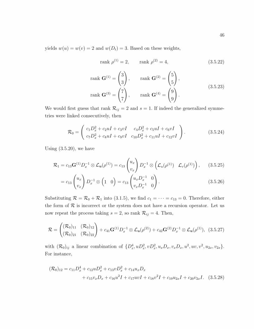
46

yields w(u) = w(v) = 2 and w(Dt) = 3. Based on these weights,

rank ρ(1) = 2, rank ρ(2) = 4, (3.5.22)

rank G(1) =

(3

3

), rank G(2) =

(5

5

),

rank G(3) =

(7

7

), rank G(4) =

(9

9

).

(3.5.23)

We would first guess that rank Rij = 2 and s = 1. If indeed the generalized symme-

tries were linked consecutively, then

R0 =

(c1D

2x + c2uI + c3vI c4D

2x + c5uI + c6vI

c7D2x + c8uI + c9vI c10D

2x + c11uI + c12vI

). (3.5.24)

Using (3.5.20), we have

R1 = c13G(1)D−1

x ⊗ Lu(ρ(1)) = c13

(ux

vx

)D−1

x ⊗(Lu(ρ

(1)) Lv(ρ(1))

), (3.5.25)

= c13

(ux

vx

)D−1

x ⊗(1 0

)= c13

(uxD

−1x 0

vxD−1x 0

). (3.5.26)

Substituting R = R0 +R1 into (3.1.5), we find c1 = · · · = c13 = 0. Therefore, either

the form of R is incorrect or the system does not have a recursion operator. Let us

now repeat the process taking s = 2, so rank Rij = 4. Then,

R =

((R0)11 (R0)12

(R0)21 (R0)22

)+ c41G

(1)D−1x ⊗ Lu(ρ(2)) + c42G

(2)D−1x ⊗ Lu(ρ(1)), (3.5.27)

with (R0)ij a linear combination of {D4x, uD2

x, vD2x, uxDx, vxDx, u

2, uv, v2, u2x, v2x}.For instance,

(R0)12 = c11D4x + c12uD2

x + c13vD2x + c14uxDx

+ c15vxDx + c16u2I + c17uvI + c18v

2I + c19u2xI + c20v2xI. (3.5.28)

47

Using (3.5.20), the first term of R1 in (3.5.27) is

R(1)1 = c41G

(1)D−1x ⊗ Lu(ρ(2)) = c41

(ux

vx

)D−1

x ⊗(6uI −4vI

)

= c41

(3uxD

−1x uI −2uxD

−1x vI

3vxD−1x uI −2vxD

−1x vI

).

The second term of R1 in (3.5.27) is

R(2)1 = c42G

(2)D−1x ⊗ Lu(ρ(1)) = c42

(F1(u)

F2(u)

)D−1

x ⊗(I 0

)= c42

(F1(u)D−1

x 0

F2(u)D−1x 0

).

Substituting the form of R = R0 + R1 = R0 + R(1)1 + R(2)

1 into (3.1.5), the linear

system for ci has a non-trivial solution. Solving the linear system, we finally obtain

R =

((R)11 (R)12

(R)21 (R)22

), (3.5.29)

where

(R)11 = D4x + 8uD2

x + 12uxDx + 16u2I + 8u2xI − 16

3v2I

+ 4uxD−1x uI + 12uuxD

−1x + 2u3xD

−1x − 8vvxD

−1x ,

(R)12 = −20

3vD2

x −16

3vxDx − 16

3uvI − 4

3v2xI − 8

3uxD

−1x vI

(R)21 = −10vxDx − 12v2xI + 4vxD−1x uI − 12uvxD

−1x − 4v3xD

−1x ,

(R)22 = −4D4x − 16uD2

x − 8uxDx − 16

3v2I − 8

3vxD

−1x vI.

Again, (3.5.29) generates infinitely many generalized symmetries from any generalized

symmetry, establishing that (2.3.33) is completely integrable.

3.6 Implementation

In this section, we present the details of the steps of the algorithm for (3.1.1), a

polynomial systems of M evolution equations in (1 + 1) dimensions. We assume that

48

any constant coefficients parameterizing the system are nonzero.

As a running example of (3.1.1), consider the dispersiveless long wave system [1],

ut = uvx + uxv

vt = ux + vvx,(3.6.1)

which describe shallow water waves.

3.6.1 Algorithm for building the candidate recursion operator

Step 1 (Find the dilation symmetry). The dilation symmetry is found by requiring

that each equation in (3.1.1) is uniform in rank; an equation is uniform in rank if

every monomial in that equation has the same rank. If (3.1.1) is not uniform in rank,

we multiply those terms that are not uniform in rank by a weighted parameter which

will later be set equal to one.

Since the linear system for the weights is always underdetermined, we set w(Dx) =

1 and this (typically) fixes the values for the remaining weights; if the linear system is

still underdetermined, the user must supply additional information to fix the weights

before the algorithm can continue.

For (3.6.1), we have the linear system

w(u) + w(Dt) = w(u) + w(v) + 1 = w(u) + w(v) + 1,

w(v) + w(Dt) = w(u) + 1 = 2w(v) + 1.(3.6.2)

Thus, 2w(v) = w(u), w(Dt) = w(v) + 1, and w(Dx) = 1. If we take w(u) = 2, then

the scaling symmetry for (3.6.1) becomes

(t, x, u, v) → (λ−2t, λ−1x, λ2u, λv). (3.6.3)

Step 2 (Determine the rank of the recursion operator). To determine the rank of the

recursion operator, we compute the first s + 1 generalized symmetries and then use

rank Rij = rank G(k+s)i − rank G

(k)j (3.6.4)

49

to determine the rank of R. Since the gap s cannot be determined a priori, we assume

s = 1 unless otherwise specified by the user.

For (3.6.1), the first two generalized symmetries and their ranks are

G(1) =

(ux

vx

), rankG(1) =

(3

2

), (3.6.5)

G(2) =

(uvx + vux

ux + vvx

), rankG(2) =

(4

3

). (3.6.6)

Thus, using (3.6.4), we compute the rank matrix for R :

rankR =

(1 2

0 1

). (3.6.7)

Step 3 (Generate the local differential operator, R0). Given the rank of the recursion

operator, we take a linear combination of

Dk0x uk1

1 uk22 · · · ukM

M αkM+1βkM+2 · · · , k0, k1, . . . ∈ Z∗, (3.6.8)

where the ki are taken so the monomial has the correct rank, the operator Dx has

been propagated to the right, and α, β, . . . are the weighted parameters from Step 1

(if present).

For (3.6.1), our local differential operator is

R0 =

(c1Dx + c2vI c3D

2x + c4uI + c5vDx + c6v

2I + c7vxI

c8I c9Dx + c10vI

). (3.6.9)

Step 4 (Generate the non-local integral operator, R1). Since the non-local operator

involves the outer product of generalized symmetries and cosymmetries, we compute

the conserved densities up to

maxi,j{rankRij − rank(G(1))i + w(uj) + w(Dx)}. (3.6.10)

We add w(uj) in (3.6.10) because the Euler operator Lujdecreases the weight of the

50

conserved density by the weight of uj. In most cases, we take a linear combination of

the terms

G(i)D−1x ⊗ Lu(ρ(j)), i, j ∈ Z∗, (3.6.11)

of the correct rank as the candidate non-local operator. However, there are cases

in which we must take a linear combination of the monomials in each term of type

(3.6.11).

For (3.6.1), we only need the first conserved density ρ(1) = v. The first cosymmetry

is then

Lu(ρ(1)) =(0 I

), (3.6.12)

and

G(1)D−1x ⊗ Lu(ρ(1)) =

(0 uxD

−1x

0 vxD−1x

). (3.6.13)

Thus, the non-local operator is

R1 =

(0 c11uxD

−1x

0 c12vxD−1x

). (3.6.14)

Step 5 (Add the local and the non-local operators to form R). The candidate recursion

operator is

R = R0 +R1. (3.6.15)

So, the candidate recursion operator for (3.6.1) is

R =

(c1Dx + c2vI c3D

2x + c4uI + c5vDx + c6v

2I + c7vxI + c11uxD−1x

c8I c9Dx + c10vI + c12vxD−1x

). (3.6.16)

3.6.2 Algorithm for determining the unknown coefficients

Step 1 (Compute the terms in the defining equation). While the computation of the

terms in the defining equation is fairly straightforward, it is computationally intensive

and prone to error when done by hand. Both the Kaup-Kupershmidt equation and

Hirota-Satsuma system would take weeks to do by hand and fill forty or fifty pages

with computations. Therefore, besides testing the recursion operators automatically

51

generated by the methods in Section 3.6.1, we also allow the testing of any recursion

operator for (3.1.1) which is computed by hand, found in the literature, etc.

In general, computer algebra systems are only designed to quickly and efficiently

work with commutative algebraic structures. Thus, the implementation of the defin-

ing equation is only possible after the properties of integro-differential operators in

Section 3.2 have been carefully implemented.

Step 1.1 (Compute Rt). The computation of Rt is easy. Since our candidate

recursion operator is t-independent, Rt = 0.

Step 1.2 (Compute R′[F(u)]). The Frechet derivative of R in the direction of

F(u) is

R′[F(u)] =m∑

k=0

(Dk

xF(u)) ∂R

∂ukx

. (3.6.17)

Unlike the Frechet derivative (3.1.3) of F(u) in the direction of G (used in the com-

putation of generalized symmetries), R and F(u) must be computed as operators in

(3.6.17).

For (3.6.1),

R′[F(u)] =

((R′[F(u)])11 (R′[F(u)])12

(R′[F(u)])21 (R′[F(u)])22

)(3.6.18)

where

(R′[F(u)])ij =m∑

k=0

(Dk

xF(u)) ∂(R)ij

∂ukx

. (3.6.19)

and

(R′[F(u)])11 = c2(ux + vvx)I, (3.6.20)

(R′[F(u)])21 = 0, (3.6.21)

(R′[F(u)])12 = +c5(ux + vvx)Dx +(c4uvx + (2c6 + c4)vux + 2c6v

2vx (3.6.22)

+ c7vv2x + c7v2x + c7u2x

)I + c11(2uxvx + uv2x + vu2x)D

−1x ,

(R′[F(u)])22 = c10(ux + vvx)I + c12(u2x + vv2x + v2x)D

−1x . (3.6.23)

Step 1.3 (Compute F′(u)). Use the formula (3.1.7) to compute F′(u).

52

For (3.6.1),

F′(u) =

(vDx + vxI uDx + uxI

Dx vDx + vxI

). (3.6.24)

Step 1.4 (Compose R and F′(u)). The composition of the M × M matrices Rand F′(u) is an order preserving inner product of the two matrices.

In the case of (3.6.1),

R ◦ F′(u) =

((R ◦ F′(u))11 (R ◦ F′(u))12

(R ◦ F′(u))21 (R ◦ F′(u))22

), (3.6.25)

with

(R ◦ F′(u))11 = c3D3x + (c1 + c5)vD2

x +(2c1vx + c2v

2 + c4u + c6v2 (3.6.26)

+ c7vx

)Dx + (c1v2x + c2vvx + c11ux)I,

(R ◦ F′(u))12 = c3vD3x + (c1u + 3c3vx + c5v

2)D2x +

(2c1ux + c2uv + 3c3v2x (3.6.27)

+ c4uv + 2c5vvx + c6v3 + c7vvx

)Dx +

(c1u2x + c2vux

+ c3v3x + c4uvx + c5vv2x + c6v2vx + c7v

2x + c11vux

)I,

(R ◦ F′(u))21 = c9D2x + (c8 + c10)vDx + (c8 + c12)vxI, (3.6.28)

(R ◦ F′(u))22 = c9vD2x + (c8u + 2c9vx + c10v

2)Dx +(c8ux + c9v2x (3.6.29)

+ c10vvx + c12vvx

)I.

Similarly,

F′(u) ◦ R =

((F′(u) ◦ R)11 (F′(u) ◦ R)12

(F′(u) ◦ R)21 (F′(u) ◦ R)22

), (3.6.30)

with

(F′(u) ◦ R)11 = c1vD2x + (c1vx + c2v

2 + c8u)Dx + (2c2vvx + c8ux)I, (3.6.31)

53

(F′(u) ◦ R)12 = c3vD3x + (c3vx + c5v

2 + c9u)D2x +

(c4uv + 2c5vvx + c6v

3 (3.6.32)

+ c7vvx + c9ux + c10uv)Dx +

(c4uvx + c4vux + 3c6v

2vx

+ c7v2x + c7vv2x + c10uvx + c10vux + c11vux + c12uvx

)I

+ (c11uxvx + c11vu2x + c12uv2x + c12uxvx)D−1x ,

(F′(u) ◦ R)21 = c1D2x + (c2 + c8)vDx + (c2 + c8)vxI, (3.6.33)

(F′(u) ◦ R)22 = c3D3x + (c5 + c9)vD2

x +(c4u + c5vx + c6v

2 + c7vx (3.6.34)

+ c9vx + c10v2)Dx +

(c4ux + 2c6vvx + c7v2x + 2c10vvx

+ c11ux + c12vvx

)I + (c11u2x + c12vv2x + c12v

2x)D

−1x .

Step 1.5 (Sum the terms in the defining equation). For (3.6.1), summing the terms

in the defining equation we find

c3D3x + c5vD2

x + (c1 + c7)vxDx + (c4 − c8)uDx + c6v2Dx

+ (c2 − c8 + c11)uxI + c1v2xI ≡ 0, (3.6.35)

(c1 − c9)uD2x + 2c3vxD

2x + (c2 − c10)uvDx + (c5 − c9 + 2c1)uxDx

+ c5vvxDx + 3c3v2xDx − (c1 − c7)u2xI + (c4 − c10 − c12)uvxI

+ (c2 + 2c6 − c10)vuxI + c5vv2xI + c7v2xI + c3v3xI

+ (c11 − c12)uv2xD−1x + (c11 − c12)uxvxD

−1x ≡ 0, (3.6.36)

(c1 − c9)D2x + (c2 − c10)vDx + (c2 − c12)vxI ≡ 0, (3.6.37)

c3D3x + c5vD2

x + (c4 − c8)uDx + (c5 + c7 − c9)vxDx

+ c6v2Dx + (c4 − c8 − c10 + c11)uxI + 2c6vvxI

+ (c7 − c9)v2xI + (c11 − c12)u2xD−1x ≡ 0. (3.6.38)

Step 2 (Extract the linear system for the unknown coefficients). Group the terms in

like powers of u,ux,uxx, . . . , I,Dx, D2x, . . . and D−1

x . Then, requiring that the expres-

sions are identically equal to zero gives us a linear system for the unknown coefficients.

54

For (3.6.1), we obtain

c1 = 0, c3 = 0, c5 = 0, c6 = 0, c7 = 0, c4 − c8 = 0,

c1 − c9 = 0, 2c1 + c5 − c9 = 0, c5 + c7 − c9 = 0,

c2 − c10 = 0, c2 + 2c6 − c10 = 0, c2 − c10 = 0,

c4 − c8 − c10 + c11 = 0, c2 − c8 + c11 = 0, c4 − c10 − c12 = 0,

c11 − c12 = 0, −c2 + c12 = 0, −c11 + c12 = 0.

(3.6.39)

Step 3 (Solve the linear system and build the recursion operator). Solve the linear

system and substitute the constants into the candidate recursion operator.

For (3.6.1), we find

c1 = c3 = c5 = c6 = c7 = c9 = 0, 2c2 = c4 = 2c10 = 2c11 = 2c12 = c8, (3.6.40)

so taking c8 = 2 gives

R =

(vI 2uI + uxD

−1x

2I vI + vxD−1x

). (3.6.41)

The recursion operator allows one to generate infinitely many generalized symmetries

of (3.6.1), establishing its completely integrable.

3.7 Other Software Packages

There has been little work on using computer algebra methods to find and test re-

cursion operators. To our knowledge, our package PDERecursionOperator.m is the

only fully automated software package for finding and testing recursion operators.

Fuchssteiner et al. [16] wrote both a Maple and a Macsyma package for testing

recursion operators in 1987; while these packages could verify if a recursion operator

is correct, it was unable to either generate the form of the operator or test a can-

didate recursion operator with unknown coefficients. Bilge [7] did substantial work

on finding recursion operators interactively with Reduce. Sanders and Wang [42, 46]

wrote software in Maple and Form to aid in their computation of recursion operators.

Recently, Meshkov [33] implemented a package in Maple for investigating complete

55

integrability from the geometric perspective; if the zero curvature representation of

the system is known, then the software package can compute the recursion operator.

3.8 Additional Examples

3.8.1 Nonlinear Schrodinger equation

For convenience, we write the standard nonlinear Schrodinger equation (NLS),

iut + uxx + 2|u|2u = 0, (3.8.1)

as the system

ut + uxx + 2u2v = 0,

vt − vxx − 2uv2 = 0,(3.8.2)

where v = u and i has been absorbed into the scale of t.

To determine the weights, we assume w(u) = w(v) so that the dilation symmetry

is (u, v, x, t) → (λ2u, λ2v, λ−1x, λ−2t). The first couple generalized symmetries and

conserved densities are

G(1) =

(−u

v

), G(2) =

(ux

vx

), (3.8.3)

ρ(1) = uv, ρ(2) = uxv. (3.8.4)

Thus, rankRij = 1 and the candidate local operator is

R0 =

(c1Dx + (c2u + c3v)I c4Dx + (c5u + c6v)I

c7Dx + (c8u + c9v)I c10Dx + (c11u + c12v)I

). (3.8.5)

The non-local operator is

R1 = G(1)D−1x ⊗ Lu(ρ(1)) =

(−c13uD−1

x v −c14uD−1x u

c15vD−1x v c16vD−1

x u

). (3.8.6)

Substituting R0 +R1 into (3.1.5), solving for the undetermined coefficients, and

56

taking c16 = −2, we find

R =

(Dx + 2uD−1

x v 2uD−1x u

−2vD−1x v −Dx +−2vD−1

x u

). (3.8.7)

Therefore, with (3.8.7) we can construct an infinite sequence of generalized symme-

tries and (3.8.2) is completely integrable.

3.8.2 Burgers’ equation

Consider the Burgers’ equation [36],

ut = u2x + uux, (3.8.8)

which has the dilation symmetry (u, x, t) → (λu, λ−1x, λ−2t). The first couple gener-

alized symmetries and conserved densities of (3.8.8) are

G(1) = ux, G(2) = uxx + uux, ρ(1) = u. (3.8.9)

Thus, rankR = 1 and the candidate recursion operator is

R = c1Dx + c2uI + c3G(1)D−1

x Lu(ρ(1)) = c1Dx + c2uI + c3uxD

−1x . (3.8.10)

Using the defining equation (3.1.5), we determine that c1 = 2c3 and c2 = c3. Taking

c2 = 12, gives the recursion operator found in [35],

R = Dx +1

2uI +

1

2uxD

−1x . (3.8.11)

The Burgers’ equation also has the recursion operator [36],

R = tR+1

2x +

1

2D−1

x = tDx +1

2(tu + x) +

1

2(tux + 1) D−1

x , (3.8.12)

which explicitly depends on x and t. To find recursion operators that depend explicitly

on x and t, we can again use scaling symmetries to build R. First, we must assume

a maximum degree in x and t; for instance, we might allow x and t but not x2 or t2.

57

The local candidate operator is then

R0 = c1tDx + (c2x + c3tu)I. (3.8.13)

The first symmetries that explicitly depend on x and t are

G(1) = 1 + tux, G(2) =1

2(u + xux) + tuux + tuxx. (3.8.14)

Thus, the non-local candidate operator is

R1 = c4G(1)D−1

x Lu(ρ(1)) = c4(tux + 1)D−1

x . (3.8.15)

Requiring the Lie derivative of R0 + R1 is zero and taking c4 = 12

gives the recursion

operator in (3.8.12).

3.8.3 Drinfel’d-Sokolov-Wilson equation

Consider the Drinfel’d-Sokolov-Wilson system [1, 25],

ut = 3vvx,

vt = 2v3x + 2uvx + uxv,(3.8.16)

which has static soliton solutions that interact with moving solitons without defor-

mation.

The scaling symmetry for (3.8.16) is (u, v, x, t) → (λ2u, λ2v, λ−1x, λ−3t). The first

few generalized symmetries and conserved densities are

G(1) =

(ux

vx

), G(2) =

(3vvx

uxv + 2uvx + 2v3x

), (3.8.17)

ρ(1) = u, ρ(2) = v2, ρ(3) =4

27u3 − 2

3uv2 − 1

9u2

x + v2x. (3.8.18)

Interestingly, the gap s = 3 and rankRij = 6. So, the local candidate operator

58

has elements involving D6x. For example,

(R0)11 = c1D6x + (c2u + c5v)D4

x + (c8ux + c10vx)D3x + (c3u

2 + c6v2 + c12u2x

+ c13v2x + c18uv)D2x + (c14u3x + c15v3x + c20uux + c21uvx + c25vux + c26vvx)Dx

+ (c4u3 + c7v

3 + c27vu2x + c28vv2x + c29uxvx + c9u2x + c11v

2x + c16u4x

+ c17v4x + c19uv2 + c22uu2x + c23uv2x + c24u2v)I. (3.8.19)

The non-local operator is

R1 =4∑

i=1

G(i)D−1x ⊗ Lu(ρ(5−i)) =

((R1)11 (R1)12

(R1)21 (R1)22

), (3.8.20)

where

(R1)11 = −1

9c117u5xD

−1x − 25

18c118uxu2xD

−1x − 5

9c119uu3xD

−1x (3.8.21)

− 5

9c120u

2uxD−1x +

5

6c121v

2uxD−1x +

5

3c122vv3xD

−1x +

5

2c123vxv2xD

−1x

− 2

3c124uxD

−1x v2 +

2

9c125uxD

−1x u2x +

4

9c126uxD

−1x u2 +

5

3c127uvvxD

−1x ,

(R1)12 = −2c128uxD−1x v2x − 4

3c129uxD

−1x uv + 3c130vvxD

−1x v, (3.8.22)

(R1)21 = c131v5xD−1x +

5

9c132u

2vxD−1x +

5

9c133vu3xD

−1x +

5

6c134v

2vxD−1x (3.8.23)

+5

3c135uv3xD

−1x +

35

18c136vxu2xD

−1x +

5

2c137uxv2xD

−1x − 2

3c138vxD

−1x v2

+2

9c139vxD

−1x u2x +

4

9c140vxD

−1x u2 +

5

9c141uvuxD

−1x ,

(R1)22 = −2c142vxD−1x v2x + 2c143v3xD

−1x v + 2c144uvxD

−1x v (3.8.24)

− 4

3c145vxD

−1x uv + c146vuxD

−1x v.

The terms in (3.1.5) fill 160 pages and grouping like terms results in a system of

508 linear equations for ci. Solving these linear equations and taking c146 = −9, gives

the recursion operator

R =

((R)11 (R)12

(R)21 (R)22

)(3.8.25)

59

where

(R)11 = D6x + 6uD4

x + 42uxD3x +

(9u2 − 21v2 +

229

2u2x

)D2

x (3.8.26)

+(66uux − 159vvx +

289

2u3x

)Dx +

(4u3 − 12uv2 +

137

2uu2x +

145

2u4x

+261

4u2

x −345

2vv2x − 609

4v2

x

)I +

(5u2ux + 5uu3x − 15uvvx − 15vv3x − 15

2v2ux

+25

2uxu2x − 45

2vxv2x + u5x

)D−1

x +1

2uxD

−1x u2x − 3

2uxD

−1x v2 + uxD

−1x u2,

(R)12 = −42vD4x − 219vxD

3x −

(48uv +

873

2v2x

)D2

x −(129uvx + 156vux (3.8.27)

+789

2v3x

)Dx −

(18v3 + 204uxvx + 6u2v +

177

2uv2x +

255

2vu2x +

273

2v4x

)I

− 27vvxD−1x v − 3uxD

−1x uv − 9

2uxD

−1x v2x,

(R)21 = −14vD4x − 123vxD

3x −

(16uv +

813

2v2x

)D2

x −(50vux + 85uvx (3.8.28)

+1219

2v3x

)Dx −

(149uxvx + 2u2v + 6v3 +

237

2uv2x +

723

2v4x +

95

2vu2x

)I

−(15uv3x + 5u2vx + 5uvux + 5vu3x + 9v5x +

15

2v2vx +

35

2vxu2x

+45

2uxv2x

)D−1

x +1

2vxD

−1x u2x − 3

2vxD

−1x v2 + vxD

−1x u2,

(R)22 = −27D6x − 54uD4

x − 324uxD3x −

(27u2 + 33v2 +

1539

2u2x

)D2

x (3.8.29)

−(162uux + 237vvx +

1701

2u3x

)Dx −

(24uv2 +

243

2uu2x +

459

4u2

x

+489

2vv2x +

729

2u4x +

885

4v2

x

)I − 9

(2uvx + 2v3x + vux

)D−1

x v

− 3vxD−1x uv − 9

2vxD

−1x v2x

To our knowledge, this recursion operator which was computed with PDERecursion-

Operator.m has not been found before.

This example shows the importance of computer algebra software in the study

of integrability; the sheer length of the computations make it almost impossible to

compute the recursion operators for all but the simplest systems by hand.

60

CHAPTER 4

CONCLUSION AND FUTURE WORK

The Painleve test is applicable to polynomial systems of ODEs and PDEs. While the

Painleve test does not prove integrability, it helps to identify candidates for complete

integrability in a surprisingly straightforward manner. For differential equations with

parameters (including arbitrary functions), our software allows the user to determine

the conditions under which the system may possess the Painleve property. Therefore,

by finding the compatibility conditions, classes of parameterized differential equations

can be analyzed to find the candidates for complete integrability.

The difficulty in completely automating the Painleve test lies in determining the

dominant behavior of the Laurent series solutions; specifically, determining all the

valid dominant behaviors when one or more of the αi are undetermined. While there

are other implementations for the Painleve test, they are either limited to ODEs

or in the complexity of the PDEs they can test. Ours is the only implementation

in Mathematica which allows the testing of systems of polynomial PDEs with no

limitations on the size of the system or the number of independent variables.

To our knowledge, no one has ever attempted to fully automate an algorithm for

finding or testing recursion operators. The commutative nature of computer algebra

systems makes it a non-trivial task to efficiently implement the non-commutative

rules needed for working with integro-differential operators.

By finding recursion operators, polynomial PDEs which can be written in evolu-

tion form, ut = F(u,ux, . . . ,umx) with constant coefficients, can be tested for com-

plete integrability in a straightforward manner. While our implementation for finding

and testing recursion operators can find the necessary constraints on the parameters,

it is not as robust at finding these constraints as the Painleve test. Therefore, it is

often advantageous to test a system of nonlinear evolution equations for the Painleve

property before attempting to find its recursion operator (if it exists).

With the tools developed for finding and testing recursion operators, it would be

possible to extend the algorithm to find cosymplectic, symplectic and even conjugate

61

recursion operators, and master symmetries. A symplectic operator maps generalized

symmetries into cosymmetries, while a cosymplectic operator maps cosymmetries into

generalized symmetries. Hence, the recursion operator for a system is the composition

of the cosymplectic operator and the symplectic operator of the system. A conjugate

recursion operator maps conserved densities of lower order to conserved densities of

higher order. The master symmetry can be used to generate an infinite hierarchy of

time-dependent generalized symmetries. It would also be worthwhile to extend our

algorithm to find recursion operators which explicitly dependend on time.

62

LIST OF ABBREVIATIONS

PDEs – Partial Differential Equations . . . . . . . . . . . . . . . . . . . . . 1

IST – Inverse Scattering Transform . . . . . . . . . . . . . . . . . . . . . . 1

ODEs – Ordinary Differential Equations . . . . . . . . . . . . . . . . . . . 2

ARS – Ablowitz, Ramani and Segur . . . . . . . . . . . . . . . . . . . . . . 3

WTC – Weiss, Tabor and Carnevale . . . . . . . . . . . . . . . . . . . . . 4

KdV – Korteweg-de Vries . . . . . . . . . . . . . . . . . . . . . . . . . . . 4

FPU – Fermi, Pasta and Ulam . . . . . . . . . . . . . . . . . . . . . . . . . 4

mKdV – Modified Korteweg-de Vries . . . . . . . . . . . . . . . . . . . . . 7

NLS – Nonlinear Schrodinger . . . . . . . . . . . . . . . . . . . . . . . . . 32

KK – Kaup-Kupershmidt . . . . . . . . . . . . . . . . . . . . . . . . . . . 43

63

REFERENCES CITED

[1] M. J. Ablowitz and P. A. Clarkson. Solitons, Nonlinear Evolution Equations andInverse Scattering. Cambridge University Press, Cambridge, 1991.

[2] M. J. Ablowitz, A. Ramani, and H. Segur. A connection between nonlinearevolution equations and ordinary differential equations of P -type. I. J. Math.Phys., 21(4):715–721, 1980.

[3] M. J. Ablowitz, A. Ramani, and H. Segur. A connection between nonlinearevolution equations and ordinary differential equations of P -type. II. J. Math.Phys., 21(5):1006–1015, 1980.

[4] D. Baldwin and W. Hereman. PainleveTest.m: A Mathematica package for thePainleve test of systems of ODEs and PDEs, 2003.

[5] D. Baldwin and W. Hereman. PDERecursionOperator.m: A Mathematica pack-age for the symbolic computation of recursion operators for nonlinear partialdifferential equations, 2004.

[6] D. Baldwin, W. Hereman, and J. Sayers. Symbolic algorithms for the Painlevetest, special solutions, and recursion operators for nonlinear PDEs. In D. Leviand P. Winternitz, editors, CRM Proceedings for the Workshop on Group Theoryand Numerical Methods. AMS, 2004.

[7] A. H. Bilge. On the equivalence of linearization and formal symmetries as inte-grability tests for evolution equations. J. Phys. A: Math. Gen., 26:7511–7519,1993.

[8] P. J. Caudrey, R. K. Dodd, and J. D. Gibbon. A new hierarchy of korteweg-devries equations. Proc. Roy. Soc. Lond. A, 351:407–422, 1976.

[9] A. R. Chowdhury. Painleve Analysis and its Applications, volume 105 of Mono-graphs and Surveys in Pure and Applied Mathematics. Chapman & Hall/CRC,Boca Raton, 2000.

[10] R. Conte. Singularities of differential equations and integrability. In D. Ben-est and C. Froeschle, editors, Introduction to Methods of Complex Analysis andGeometry for Classical Mechanics and Non-Linear Waves, pages 49–143. Gif-sur-Yvette: Editions Frontieres, 1993.

64

[11] R. Conte, editor. The Painleve Property: One Century Later. CRM Series inMathematical Physics. Springer, New York, 1999.

[12] R. Conte, A. P. Fordy, and A. Pickering. A perturbative Painleve approach tononlinear differential equations. Physica, 69D:33–58, 1993.

[13] R. K. Dodd, J. C. Eilbeck, J. D. Gibbon, and M. C. Morris. Solitons andNonlinear Wave Equations. Academic Press, London, 1982.

[14] A. S. Fokas. Symmetries and integrability. Stud. Appl. Math., 77:253–299, 1987.

[15] A. P. Fordy and J. Gibbons. Some remarkable nonlinear transformations. Phys.Lett. A, 75(5):325, 1980.

[16] B. Fuchssteiner, W. Oevel, and W. Wiwianka. Computer-algebra methods forinvestigation of hereditary operators of higher order soliton equations. Comp.Phys. Comm., 44:47–55, 1987.

[17] C. S. Gardner, J. M. Greene, M. D. Kruskal, and R. M. Miura. Method forsolving the Korteweg-de Vries equation. Phys. Rev. Lett., 19:1095–1097, 1967.

[18] U. Goktas. Algorithmic Computation of Symmetries, Invariants and RecursionOperators for Systems of Nonlinear Evolution and Differential-Difference Equa-tions. PhD thesis, Colorado School of Mines, Golden, Colorado, May 1998.

[19] U. Goktas and W. Hereman. Mathematica package InvariantSymmetries.mis available since 1997 from http://www.mathsource.com/cgi-bin/msitem?0208-932.

[20] U. Goktas and W. Hereman. Symbolic computation of conserved densities forsystems of nonlinear evolution equations. J. Symb. Comp., 24:591–621, 1997.

[21] U. Goktas and W. Hereman. Algorithmic computation of higher-order symme-tries for nonlinear evolution and lattice equations. Adv. Comp. Math., 11:55–80,1999.

[22] B. Grammaticos and A. Ramani. Integrability – and how to detect it. InY. Kosmann-Schwarzbach, B. Grammaticos, and K. Tamizhmani, editors, In-tegrability of Nonlinear Systems, pages 30–94. Springer-Verlag, Berlin, 1997.

[23] W. Hereman and U. Goktas. Integrability tests for nonlinear evolution equations.In M. Wester, editor, Computer Algebra Systems: A Practical Guide, pages 211–232. Wiley, New York, 1999.

65

[24] W. Hereman, U. Goktas, M. D. Colagrosso, and A. J. Miller. Algorithmic in-tegrability tests for nonlinear differential and lattice equations. Comp. Phys.Comm., 115:428–446, 1998.

[25] R. Hirota, B. Grammaticos, and A. Ramani. Soliton structure of the drinfel’d-sokolov-wilson equation. J. Math. Phys., 27(6):1499–1505, 1986.

[26] R. Hirota and A. Ramani. The miura transformations of kaup’s equation and ofmikhailov’s equation. Phys. Lett. A, 76(2):95–96, 1980.

[27] E. L. Ince. Ordinary Differential Equations. Dover, New York, 1944.

[28] R. S. Johnson. On solutions of the Camass-Holm equation. Proc. Roy. Soc.Lond. A, 459:1687–1708, 2003.

[29] M. Lakshmanan and P. Kaliappan. Lie transformations, nonlinear evolutionequations, and Painleve forms. J. Math. Phys., 24(4):795–806, 1983.

[30] G. L. Lamb. Elements of soliton theory. Wiley, New York, 1980.

[31] P. Lax. Integrals of nonlinear equations of evolution and solitary waves. Comm.Pure Appl. Math., 21:467–490, 1968.

[32] J. B. McLeod and P. J. Olver. The connection between partial differential equa-tions soluble by inverse scattering and ordinary differential equations of Painlevetype. SIAM J. Math. Anal., 14(3):488–506, 1983.

[33] A. G. Meshkov. Computer package for investigation of the complete integrability.In Proceedings of Institute of Mathematics of NAS of Ukraine, volume 30, pages35–46. 2000.

[34] A. C. Newell. Solitons in Mathematics and Physics, volume 48 of CBMS-NSFRegional Conference Series in Applied Mathematics. SIAM, Philadelphia, 1985.

[35] P. J. Olver. Evolution equations possessing infinitely many symmetries. J. Math.Phys., 18(6):1212–1215, 1977.

[36] P. J. Olver. Applications of Lie groups to Differential Equations, volume 107of Graduate Texts in Mathematics. Springer-Verlag, New York, second edition,1993.

[37] W. F. Osgood. Topics in the theory of functions of several complex variables. InThe Madison Colloquium 1913, volume 4 of Colloquium Lectures, pages 111–230.AMS, New York, 1914.

66

[38] P. Painleve. Memoire sur les equations diffrentielles dont l’integrale generale estuniforme. Bull. Soc. Math. France, 28:201–261, 1900.

[39] A. Ramani, B. Grammaticos, and T. Bountis. The Painleve property and singu-larity analysis of integrable and nonintegrable systems. Phys. Rep., 180(3):159–245, 1989.

[40] D. W. Rand and P. Winternitz. ODEPAINLEVE – a Macsyma package forPainleve analysis of ordinary differential equations. Comp. Phys. Comm., 42:359–383, 1986.

[41] F. Renner. A constructive REDUCE package based upon the Painleve analysisof nonlinear evolutions equations in Hamiltonian and/or normal form. Comp.Phys. Comm., 70:409–416, 1992.

[42] J. Sanders and J. P. Wang. Combining Maple and Form to decide on integrabilityquestions. Comp. Phys. Comm., 115:447–459, 1998.

[43] C. Scheen. Implementation of the Painleve test for ordinary differential equa-tions. Theor. Comp. Sci., 187:87–104, 1997.

[44] W.-H. Steeb and N. Euler. Nonlinear evolution equations and Painleve test.World Scientific, Singapore, 1988.

[45] H.-W. Tam, X.-B. Hu, and D.-L. Wang. Two integrable coupled nonlinear sys-tems. J. Phys. Soc. Japan, 68(2):369–379, 1999.

[46] J. P. Wang. Symmetries and Conservation Laws of Evolution Equtions. PhDthesis, Thomas Stieltjes Institute for Mathematics, Amsterdam, Sept. 1998.

[47] R. S. Ward. The Painleve property for the self-dual gauge-field equations. Phys.Lett., 102A(7):279–282, 1984.

[48] J. Weiss. A compendium of unusual psi-series for partial differential equations.1988.

[49] J. Weiss, M. Tabor, and G. Carnevale. The Painleve property for partial differ-ential equations. J. Math. Phys., 24:522–526, 1983.

[50] F. Xie and Y. Chen. An algorithmic method in Painleve analysis of PDE. Comp.Phys. Comm., 154:197–204, 2003.

[51] G.-Q. Xu and Z.-B. Li. A Maple package for the Painleve test of nonlinear partialdifferential equations. Chin. Phys. Lett., 20(7):975–978, 2003.

67

[52] G.-Q. Xu and Z.-B. Li. Symbolic computation of the Painleve test for nonlinearpartial differential equations using Maple. Comp. Phys. Comm., 2004. To appear.

[53] H. Yoshida. Necessary condition for the existence of algebraic first integrals I &II. Celes. Mech., 31:363–399, 1983.

[54] S. Ziglin. Self-intersection of the complex separatrices and the nonexistence ofthe integrals in the Hamiltonian systems with one-and-half degrees of freedom.J. Appl. Math. Mech., 45:411–413, 1982.

[55] S. Ziglin. Branching of solutions and nonexistence of first integrals in Hamiltonianmechanics I. Func. Anal. Appl., 16:181–189, 1983.

[56] S. Ziglin. Branching of solutions and nonexistence of first integrals in Hamiltonianmechanics II. Func. Anal. Appl., 17:6–17, 1983.