Symbolic-Numeric Integration of Rational Functions Robert HC Moir 1 , Robert M Corless 1 , Marc Moreno Maza 1 , and Ning Xie 2 1 Ontario Research Center for Computer Algebra, University of Western Ontario, Canada 2 Huawei Technologies, Toronto, ON Abstract We consider the problem of symbolic-numeric integration of symbolic functions, fo- cusing on rational functions. Using a hybrid method allows the stable yet efficient com- putation of symbolic antiderivatives while avoiding issues of ill-conditioning to which numerical methods are susceptible. We propose two alternative methods for exact input that compute the rational part of the integral using Hermite reduction and then compute the transcendental part two different ways using a combination of exact integration and efficient numerical computation of roots. The symbolic computation is done within bpas, or Basic Polynomial Algebra Subprograms, which is a highly optimized environment for polynomial computation on parallel architectures, while the numerical computation is done using the highly optimized multiprecision rootfinding package MPSolve. We show that both methods are forward and backward stable in a structured sense and away from singularities tolerance proportionality is achieved by adjusting the precision of the rootfinding tasks. 1 Introduction Hybrid symbolic-numeric integration of rational functions is interesting for several reasons. First, a formula, not a number or a computer program or subroutine, may be desired, perhaps for further analysis such as by taking asymptotics. In this case one typically wants an exact symbolic answer, and for rational functions this is in principle always possible. However, an exact symbolic answer may be too cluttered with algebraic numbers or lengthy rational numbers to be intelligible or easily analyzed by further symbolic manipulation. See, e.g., Figure 1. Discussing symbolic integration, Kahan [7] in his typically dry way gives an example “atypically modest, out of consideration for the typesetter”, and elsewhere has rhetorically wondered: “Have you ever used a computer algebra system, and then said to yourself as screensful of answer went by, “I wish I hadn’t asked.”” Fateman has addressed rational integration [5], as have Noda and Miyahiro [8, 9], for this and other reasons. Second, there is interest due to the potential to carry symbolic-numeric methods for ra- tional functions forward to transcendental integration, since the rational function algorithm is at the core of more advanced algorithms for symbolic integration. Particularly in the con- text of exact input, which we assume, it can be desirable to have an intelligible approximate expression for an integral while retaining the exact expression of the integral for subsequent symbolic computation. The ability to do this is a feature of one of our algorithms that alternative approaches, particularly those based on partial fraction decomposition, do not share. Besides intelligibility and retention of exact results, one might be concerned with numer- ical stability, or perhaps efficiency of evaluation. We consider stability issues in Sections 4 1
Transcript
Symbolic-Numeric Integration of Rational Functions
Robert HC Moir1, Robert M Corless1, Marc Moreno Maza1, and Ning Xie2
1Ontario Research Center for Computer Algebra, University of Western Ontario, Canada2Huawei Technologies, Toronto, ON
Abstract
We consider the problem of symbolic-numeric integration of symbolic functions, fo-cusing on rational functions. Using a hybrid method allows the stable yet efficient com-putation of symbolic antiderivatives while avoiding issues of ill-conditioning to whichnumerical methods are susceptible. We propose two alternative methods for exact inputthat compute the rational part of the integral using Hermite reduction and then computethe transcendental part two different ways using a combination of exact integration andefficient numerical computation of roots. The symbolic computation is done within bpas,or Basic Polynomial Algebra Subprograms, which is a highly optimized environment forpolynomial computation on parallel architectures, while the numerical computation isdone using the highly optimized multiprecision rootfinding package MPSolve. We showthat both methods are forward and backward stable in a structured sense and awayfrom singularities tolerance proportionality is achieved by adjusting the precision of therootfinding tasks.
1 Introduction
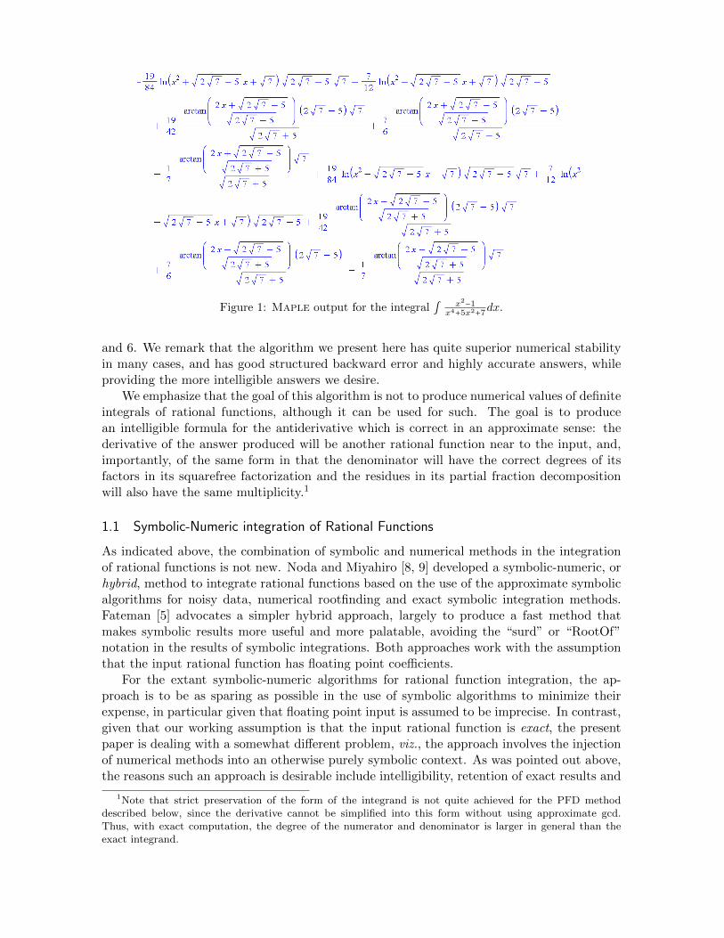
Hybrid symbolic-numeric integration of rational functions is interesting for several reasons.First, a formula, not a number or a computer program or subroutine, may be desired, perhapsfor further analysis such as by taking asymptotics. In this case one typically wants an exactsymbolic answer, and for rational functions this is in principle always possible. However,an exact symbolic answer may be too cluttered with algebraic numbers or lengthy rationalnumbers to be intelligible or easily analyzed by further symbolic manipulation. See, e.g.,Figure 1. Discussing symbolic integration, Kahan [7] in his typically dry way gives an example“atypically modest, out of consideration for the typesetter”, and elsewhere has rhetoricallywondered: “Have you ever used a computer algebra system, and then said to yourself asscreensful of answer went by, “I wish I hadn’t asked.” ” Fateman has addressed rationalintegration [5], as have Noda and Miyahiro [8, 9], for this and other reasons.
Second, there is interest due to the potential to carry symbolic-numeric methods for ra-tional functions forward to transcendental integration, since the rational function algorithmis at the core of more advanced algorithms for symbolic integration. Particularly in the con-text of exact input, which we assume, it can be desirable to have an intelligible approximateexpression for an integral while retaining the exact expression of the integral for subsequentsymbolic computation. The ability to do this is a feature of one of our algorithms thatalternative approaches, particularly those based on partial fraction decomposition, do notshare.
Besides intelligibility and retention of exact results, one might be concerned with numer-ical stability, or perhaps efficiency of evaluation. We consider stability issues in Sections 4
1
Figure 1: Maple output for the integral ∫x2−1
x4+5x2
+7dx.
and 6. We remark that the algorithm we present here has quite superior numerical stabilityin many cases, and has good structured backward error and highly accurate answers, whileproviding the more intelligible answers we desire.
We emphasize that the goal of this algorithm is not to produce numerical values of definiteintegrals of rational functions, although it can be used for such. The goal is to producean intelligible formula for the antiderivative which is correct in an approximate sense: thederivative of the answer produced will be another rational function near to the input, and,importantly, of the same form in that the denominator will have the correct degrees of itsfactors in its squarefree factorization and the residues in its partial fraction decompositionwill also have the same multiplicity.1
1.1 Symbolic-Numeric integration of Rational Functions
As indicated above, the combination of symbolic and numerical methods in the integrationof rational functions is not new. Noda and Miyahiro [8, 9] developed a symbolic-numeric, orhybrid, method to integrate rational functions based on the use of the approximate symbolicalgorithms for noisy data, numerical rootfinding and exact symbolic integration methods.Fateman [5] advocates a simpler hybrid approach, largely to produce a fast method thatmakes symbolic results more useful and more palatable, avoiding the “surd” or “RootOf”notation in the results of symbolic integrations. Both approaches work with the assumptionthat the input rational function has floating point coefficients.
For the extant symbolic-numeric algorithms for rational function integration, the ap-proach is to be as sparing as possible in the use of symbolic algorithms to minimize theirexpense, in particular given that floating point input is assumed to be imprecise. In contrast,given that our working assumption is that the input rational function is exact, the presentpaper is dealing with a somewhat different problem, viz., the approach involves the injectionof numerical methods into an otherwise purely symbolic context. As was pointed out above,the reasons such an approach is desirable include intelligibility, retention of exact results and
1Note that strict preservation of the form of the integrand is not quite achieved for the PFD methoddescribed below, since the derivative cannot be simplified into this form without using approximate gcd.Thus, with exact computation, the degree of the numerator and denominator is larger in general than theexact integrand.
stable or efficient evaluation. Since it is accuracy, speed and stability that matter in thecontext of scientific computing, a symbolic package that provides a suitable balance of thesedesiderata in a way that can be merged seamlessly with other scientific computations, as ourimplementation provides, has considerable advantages over CAS style symbolic computationwith exact roots.
The usual approach to symbolic integration here begins with a rational function f(x) =A(x)/B(x) ∈ Q(x), with deg(A) < deg(B) (ignoring any polynomial part, which can beintegrated trivially) and computes an integral in two stages:
● rational part: computes a rational function C/D such that
∫ f(x)dx =C(x)
D(x)+ ∫
G(x)
H(x)dx, (1)
where the integral on the right hand side evaluates to a transcendental function (logand arctan terms);
● transcendental part: computes the second (integral) term of the expression (1) aboveyielding, after post-processing,
∫ f(x)dx =C(x)
D(x)+∑ vi log(Vi(x)) +∑wj arctan(Wj(x)), (2)
Vi,Wj ∈ K[x], with K being some algebraic extension of Q.In symbolic-numeric algorithms for this process some steps are replaced by numeric or
quasi-symbolic methods. Noda and Miyahiro use an approximate Horowitz method (involvingapproximate squarefree factorization) to compute the rational part and either the Rothstein-Trager (RT) algorithm or (linear/quadratic) partial fraction decomposition (PFD) for thetranscendental part (see Section 2 for a brief review of these algorithms). The algorithmconsidered by Fateman avoids the two stage process and proceeds by numerical rootfindingof the denominator B(x) (with multiplicities) and PFD to compute both rational and tran-scendental parts. In both cases, the working assumption is that the input uses floating pointnumbers that are subject to uncertainty or noise and the numerical algorithms use doubleprecision.
Part of the power of symbolic algorithms is their ability to preserve structural featuresof a problem that may be very difficult to preserve numerically. Particularly given our focuson exact input, then, we are interested in preserving as much structure of the problem aspossible if we are to resort to the use of numerical methods for rootfinding. Our implemen-tation relies on the sophisticated rootfinding package MPSolve, which provides a posterioriguaranteed bounds on the relative error of all the roots for a user-specified tolerance ε. Tobalance efficiency of computation and structure-preservation, we use more efficient symbolicalgorithms where possible, such as the Hermite method for the rational part, and considertwo methods of computing the transcendental part, one that computes the exact integral us-ing the Lazard-Rioboo-Trager (LRT) method followed by numerical approximation, and theother that uses a multiprecision PFD method to compute a nearby integrand that splits overQ and then performs a structured integration. For more details on the symbolic algorithms,see Section 2. Our symbolic-numeric algorithms are discussed in Section 3.
The advantage of combining multiprecision numerical software with symbolic algorithmsis that it allows for the user to specify a tolerance on the error of the symbolic-numericcomputation. This, together with structured backward and forward error analysis of thealgorithm, then allows the result to be interpreted in a manner familiar to users of numer-ical software but with additional guarantees on structure-preservation. We provide such ananalysis of the structured error of our algorithm in Section 4.
An interesting feature of the backward stability of the algorithm is that it follows thatthe computed integral can be regarded as the exact integral of a slightly perturbed input in-tegral, and, as stated previously, of the correct form (modulo the need for approximate gcd).Insofar as the input rational function is the result of model construction or an applicationof approximation theory it is subject to error. Thus, the input, though formally exact, isnevertheless still an approximation of a system it represents. Assuming the model approx-imation error is small, this means that the “true” rational function the input represents issome nearby rational function in a small neighbourhood of f(x), for example in the sense ofthe space determined by variation of the coefficients of f . The backward stability thereforeshows that the integral actually computed is also a nearby rational function within anothersmall neighbourhood, for which we have some control over its size. In a manner similar tonumerical analysis, then, by an appropriate choice of tolerance, we can ensure that the latterneighbourhood is smaller than the former, so that the numerical perturbation of the problemis smaller than the model approximation error. The upshot of this is that the use of backwarderror analysis shows how a symbolic-numeric algorithm can be compatible with the spirit ofuncertain input, even if the input is assumed to be exact. That is, we are assuming that themodeling procedure got the “right kind” of rational function to give as input, even if its datais uncertain in other ways.
This shows how a backward error analysis can be useful even in the context of exactintegration. In the general case of exact input, however, a backward error analysis alone isnot enough. This is why we also provide a forward error analysis, to provide a posterioriassurance of a small forward error sufficiently far away from singularities in the integrand.We also provide such an analysis in Section 4.
Our algorithm may be adapted to take truly uncertain input by using additional symbolic-numeric routines, such as approximate GCD and approximate squarefree factorization, inorder to detect nearby problems with increased structure. Such an approach would shift theproblem onto the pejorative manifold (nearest most singular problem, see [6]), which protectsagainst ill-conditioning of the problem. The symbolic-numeric structured PFD integration wepropose already takes this approach. Moreover, the structured error analysis of our algorithmthen entails that the problem stays on the pejorative manifold after the computation of theintegral. Since there have been considerable advances in algorithms for approximate poly-nomial algebra since the time of writing of [9], such as the ApaTools package of Zeng [12],the combination of error control and singular problem detection could yield a considerableadvance over the early approach of Noda and Miyahiro.
2 Methods for Exact Integration of Rational Functions
We begin by reviewing symbolic methods for integrating rational functions.2 Let f ∈ R(x)be a rational function over R not belonging to R[x]. There exist polynomials P,A,B ∈ R[x]such that we have f = P + A/B with gcd(A,B) = 1 and deg(A) < deg(B). Since P isintegrated trivially, we ignore the general case and assume that f = A/B with deg(A) <
deg(B). Furthermore, thanks to Hermite reduction, one can extract the rational part of theintegral, leaving a rational function G/H, with deg(G) < deg(H) and H squarefree, remainingto integrate. For the remainder of this section, then, we will assume that the function tointegrate is given in the form G/H, with deg(G) < deg(H) and H squarefree.
2The following review is based in part on the ISSAC 1998 tutorial [3] and the landmark text book [2] ofM. Bronstein.
Partial-fraction decomposition (PFD) algorithm. The partial fraction decomposition algo-rithm for rational functions in R(x) can be presented in different ways, depending on whetherone admits complex numbers in expressions. We present a method based upon a completefactorization of the denominator over C, followed by its conversion into an expression con-taining only constants from R.
Consider the splitting of H expressed in the form
H = pn
∏i=1
(x − αi)n+m
∏j=n+1
[(x − (αj + i βj))(x − (αj − i βj))] ,
separating real roots from complex conjugate pairs, where p,αk, βk ∈ R. Then there exist akand bk such that
G
H=
n
∑i=1
aix − αi
+n+m
∑j=n+1
[aj + i bj
(x − (αj + i βj))+
aj − i bj
(x − (αj − i βj))] . (3)
The numerator quantities ck = ak + i bk corresponding to the roots γk = αk + i βk we callresidues by analogy to complex analysis. Note that in the case here where H is squarefree,the residues can be computed by the formula ck = c(γk) = G(γk)/H
′(γk).The real root terms are easily integrated to yield terms of the form ai log(x−αi). Extract-
ing terms of the form aj [(x − (αj + i βj))−1 + (x − (αj − i βj))
−1] from (3) we obtain pairs ofcomplex log terms that can be combined to form a single real log term of the form aj log(x2−
2αjx+α2j+β
2j ). Extracting terms of the form i bj [(x − (αj + i βj))
−1 − (x − (αj − i βj))−1] from
(3) and making use of the observation of Rioboo that ddx i log (X+iY
X−iY) = d
dx2 arctan(X/Y ), for
X,Y ∈ R[x] (see [2], pp. 59ff.), we obtain a term in the integral of the form 2bj arctan (αj−xβj
).
Where there are repeated residues in the PFD it is possible to combine terms of theintegral together. The combination of logarithms with common ak simply requires computingthe product of their arguments. For the arctangent terms the combination of terms withcommon bk can be accomplished by recursive application of the rule
arctan(X
Y) + arctan(
α − x
β)→ arctan(
X(α − x) − βY
Y (α − x) + βX) , (4)
which is based on the fact that log(X + i Y ) + log((α − x) + i β) = log((X(α − x) − βY ) +
i (Y (α − x) + βX)) and Rioboo’s observation noted above.A major computational bottleneck of the symbolic algorithms based on a PFD is the
necessity of factoring polynomials into irreducibles over R or C (and not just over Q) therebyintroducing algebraic numbers even if the integrand and its integral are both in Q(x). Unfor-tunately, introducing algebraic numbers may be necessary: any field containing an integral of1/(x2 + 2) contains
√2 as well. A result of modern research are so-called rational algorithms
that compute as much of the integral as can be kept within Q(x), and compute the minimalalgebraic extension of K necessary to express the integral.
The Hermite reduction. The objective is to reduce the integration of f to the case where B issquare-free without introducing any algebraic numbers. Let B = B1B
22⋯B
mm be a square-free
factorization of B. Thus, the polynomials Bi are square-free and pairwise co-prime. Assumem ≥ 2, define V ≡ Bm and U ≡ B/V m. Since gcd(UV ′, V ) = 1, we can compute C,D ∈ Q[x]such that we have
A
1 −m= CUV ′
+ DV and deg(C) < deg(V ). (5)
Elementary calculations yield
∫A
UV m=
C
V m−1+ ∫
(1 −m)D −UC ′
UV m−1. (6)
Repeated applications of equation (6) leads to the Hermite theorem which sates that one cancompute g, h ∈ Q(x), such that the denominator of h is square-free and f = g′ + h holds.
The Rothstein-Trager theorem.
It follows from the PFD of G/H, i.e., G/H = ∑ni=1 ci/(x − γi), ci, γi ∈ C, that
∫G
Hdx =
deg(H)
∑i=1
ci log(x − γi) (7)
where the γi are the zeros of H in C and the ci are the residues of G/H at the γi. Computingthose residues without splitting H into irreducible factors is achieved by the Rothstein-Tragertheorem, as follows. Since we seek roots of H and their corresponding residues given byevaluating c = G/H ′ at the roots, it follows that the ci are exactly the zeros of the Rothstein-Trager resultant R ∶= resultantx(H,G − cH
′), where c here is an indeterminate. Moreover,the splitting field of R over Q is the minimal algebraic extension of Q necessary to express
∫ f in the form given by Liouville’s theorem, i.e., as a sum of logarithms, and we have
∫G
Hdx =
m
∑i=1
∑c∣Ui(c)=0
c log(gcd(H,G − cH ′)) (8)
where R = ∏i=mi=1 U eii is the irreducible factorization of R over Q.
The Lazard-Rioboo-Trager algorithm. Consider the subresultant pseudo-remainder se-quence Ri, where R0 = R is the resultant (see p. 115 in [4]) of H and G − cH ′ w.r.t. x.Observe that the resultant R is a polynomial in c of degree deg(H), the roots of which arethe residues of G/H. Let U1U
22⋯U
mm be a square-free factorization of R. Then, we have
∫G
Hdx =
m
∑i=1
∑c∣Ui(c)=0
c log(gcd(H,G − cH ′)), (9)
which groups together terms of the PFD with common residue, as determined by the multi-plicity of Ui in the squarefree factorization. We compute the sum ∑c∣Ui(c)=0 c log(gcd(H,G−cH ′)) as follows. If all residues of H are equal, there is a single nontrivial squarefree factorwith i = deg(H) yielding ∑c∣Ui(c)=0 c log(H), otherwise, that is, if i < deg(H), the sum is
∑c∣Ui(c)=0 c log(Si), where Si = ppx(Rk), where degx(Rk) = i and ppx stands for primitivepart w.r.t. x. Consequently, this approach requires isolating only the complex roots of thesquare-free factors U1, U2, . . . , Um, whereas methods based on the PFD requires isolating thereal or complex roots of the polynomial H, where deg(H) ≥ ∑i deg(Ui). However, the co-efficients of R (and possibly those of U1, U2, . . . , Um) are likely to be larger than those ofH. Overall, depending on the example, the computational cost of root isolation may put atadvantage any of those approaches in comparison to the others.
3 The Algorithms
We consider two symbolic-numeric algorithms, both based on Hermite reduction for therational part and using two distinct methods for the transcendental part, one based on partial
fraction decomposition and the other the Lazard-Rioboo-Trager algorithm, both reviewed inSection 2. Following the notation used in equation (1), we assume the rational part C/Dhas been computed and we consider how the transcendental part is computed by the twomethods. Both algorithms use MPSolve to control the precision on the root isolation step.
Following the notations used in equation (9), the LRT-based method proceeds by com-puting the sub-resultant chain (R0,R1, . . .) and deciding how to evaluate each sum
∑c ∣Ui(c)=0
c log(Rk), deg(Rk) = i,
by applying the strategy of Lazard, Rioboo and Trager. However, we compute the complexroots of the polynomials U1, U2, . . . , Um numerically instead of representing them symbolicallyas in [11, 10]. Then, we evaluate each sum ∑c∣Ui(c)=0 c log(Rk) by an algorithm adapted tothis numerical representation of the roots. This method is presented as Algorithm 1.
The PFD-based method begins by computing numerically the roots γi of the denominatorH(x) and then computes exactly the resulting residues ci = c(γi) = G(γi)/H
′(γi). Thenumerical rootfinding can break the structure of repeated residues, which we restore bydetecting residues that differ by less than ε, the user-supplied tolerance. The resultingpartial fraction decomposition can then be integrated using the structure-preserving strategypresented in section 2 above. This strategy allows to algorithm to replicate the structure ofthe final output from the LRT algorithm as a sum of real logarithms and arctangents. Thismethod is presented as Algorithm 2.
We remark that there can be an issue here in principle as a result of roots of H that arecloser than ε. Given the properties of MPSolve, however, this is not an issue in practice,given the ability to compute residues exactly or with sufficiently high precision, becauseMPSolve isolates roots within regions where Newton’s method converges quadratically. Inthe unlikely event of residues that are distinct but within ε of each other, the algorithm stillresults in a small error and is advantageous in terms of numerical stability. This is becauseidentifying nearby roots shifts the problem onto the nearest most singular problem, the spaceof which Kahan [6] calls the pejorative manifold, which protects against ill-conditioning.
Both methods take as input a univariate rational function f(x) = A(x)/B(x) over Q withdeg(B) > deg(A), and a tolerance ε > 0. Both A(x) and B(x) are expressed in the monomialbasis. They yield as output an expression
∫ f dx =C
D+∑ vi log(Vi) +∑wj arctan(Wj), (10)
Vi,Wj ∈ Q[x], along with a linear estimate of the forward and backward error. The backwarderror on an interval [a, b] is measured in terms of ∥δ(x)∥∞ = maxa≤x≤b ∣δ(x)∣, where δ(x) =f(x)− d
dx ∫ f(x)dx, and the forward error on [a, b] is measured in terms of ∥∫ (f − f)dx∥∞ =
∥∫ δ(x)dx∥∞, where f and f ′ are assumed to have the same constant of integration. Wheref has no real singularities, we provide bounds over R, and where f has real singularities thebounds will be used to determine how close to the singularity the error exceeds the tolerance.
The main steps of Algorithm 1 and Algorithm 2 are listed below, where the numbersbetween parentheses refer to lines of the pseudo-code below. Both algorithms begin with:
(1-4:) decompose ∫ f dx into CD (rational part) and ∫
GH dx (transcendental part) using Hermite
reduction;Algorithm 1 then proceeds with:
(5-6:) compute symbolically the transcendental part ∫GH dx = ∑i∑c∣Ui(c)=0 c ⋅ log(Si(t, x))
using Lazard-Rioboo-Trager algorithm; in the pseudo-code U is a vector holding the
square-free factors of the resultant while S holds the primitive part of elements of thesub-resultant pseudo-remainder sequence corresponding to elements of U , viz., suchthat corresponding to Ui is Si = ppx(Rk), where degx(Rk) = i;
(7:) compute the roots ck of Ui(c) numerically using MPSolve to precision ε.(8-9:) symbolic post-processing in bpas: computation of the log and arctan terms.After Hermite reduction, Algorithm 2 continues with:
(5-6:) compute the roots γk of H(x) numerically using MPSolve to precision ε.(7:) compute the residues ck of G(x)/H(x) corresponding to the approximate roots of H(x)
and detect their identity within ε.(8:) compute identical residues within ε and then compute a correspondence ϕ (one-many
relation) between a representative residue and its corresponding roots. ϕ correlatesindices of selected elements of c and indices of elements of γ.
(9-10:) compute symbolically the transcendental part ∫GHdx = ∑ vi log(Vi)+
∑wj arctan(Wj) from the PFD of G(x)/H(x).Both algorithms complete the integration by processing the arctangent terms, which can
be written as arctan (XY) or arctan(X,Y ), for polynomials X and Y , after the integration
is complete, using Rioboo’s method (described in [2]) to remove spurious singularities. Theresult is the conversion of the arctangent of a rational function or two-argument arctangentinto a sum of arctangents of polynomials.Algorithm 1 symbolicNumericIntegrateLRT(f ,ε)f ∈ Q(x), ε > 0
1: (g, h)← hermiteReduce(num(f),den(f)) // Note: g, h ∈ Q(x)2: (Quo,Rem)← euclideanDivide(num(h),den(h)) // Note: Quo,Rem ∈ Q[x]3: if Quo ≠ 0 then4: P ← integrate(Quo)
5: if Rem ≠ 0 then6: (U ,S) ← integrateLogPart(Rem,den(h)) // Note: U = (Ui,1 ≤ i ≤ m) and S = (Si) are vectors with
coefficients in Q[t] and Q[t, x] respectively
7: c← rootsMP(U , ε) // Note: c = (ck) are the roots of Ui, as returned by MPSolve8: (L,A2) ← logToReal(c,S) // Note: L and A2 are, respectively, vectors of logs and two-argument arctangent
1: (g, h)← hermiteReduce(num(f),den(f)) // Note: g, h ∈ Q(x)2: (Quo,Rem)← euclideanDivide(num(h),den(h)) // Note: Quo,Rem ∈ Q[x]3: if Quo ≠ 0 then4: P ← integrate(Quo)
5: if Rem ≠ 0 then6: γ ← rootsMP(den(h), ε) // Note: γ = (γk) are the roots of den(h), as returned by MPSolve7: c← residues(Rem,den(h),γ) // Note: c = (ck) are the residues corresponding to the γi8: ϕ← residueRootCorrespondence(c,γ, ε) // Note: ϕ ⊆ N ×N9: (L,A2) ← integrateStructuredPFD(c,γ, ϕ) // Note: L and A2 are, respectively, vectors of logs and
We now consider the error analysis of the symbolic-numeric integration using LRT and PFD.We present a linear forward and backward error analysis for both methods.3
3Note that throughout this section we assume that the error for the numerical rootfinding for a polynomialP (x) satisfies the relation ∣∆r∣ ≤ ε∣r∣, where r is the value of the computed root and ∆r is the distance in the
Theorem 1 (Backward Stability). Given a rational function f = A/B satisfying deg(A) <
deg(B), gcd(A,B) = 1 and input tolerance ε, Algorithm 1 and Algorithm 2 yield an integralof a rational function f such that for ∆f = f − f ,
∥∆f∥∞ = maxx ∣∑k
Re (Ξ(x, rk))∣ +O(ε2),
where the principal term is O(ε), rk ranges over the evaluated roots and the function Ξ definedbelow is computable. This expression for the backward error is finite on any closed, boundedinterval not containing a root of B(x).
The advantage of exact computation on an approximate result is that the symbolic com-putation commutes with the approximation, i.e., we obtain the same result from issuinga given approximation and then computing symbolically as we do with computing symboli-cally first and then issuing the same approximation.4 Thus, we will conduct the error analysisthroughout this section by assuming that we have exact information and then approximateat the end.
Proof. [PFD-based backward stability] The PFD method begins by using Hermite reduction
to obtain
∫ f(x)dx =C(x)
D(x)+ ∫
G(x)
H(x)dx, (11)
where H(x) is squarefree. Given the roots γi of H(x) we may obtain the PFD of G(x)/H(x),yielding
G(x)
H(x)=
deg(H)
∑i=1
cix − γi
, (12)
where ci = c(γi) with c(x) = G(x)/H ′(x). Taking account of identical residues, the expression(12) can then be integrated using the structured PFD algorithm described in Section 2. Sincewe approximate the roots of H, we replace the exact roots γi with the approximations γi.This breaks the symmetry of the exactly repeated residues, thus the (exact) ci are modified intwo ways: by evaluating c(x) at γi; and restoring symmetry by adjusting the list of computedresidues so that residues within ε of each other are identified. This strategy requires somemethod of selecting a single representative for the list of nearby residues; the error analysisthen estimates the error on the basis of the error of this representative.5 We then representthis adjusted computed list of residues by ci. Since the Hermite reduction and PFD areequivalent to a rewriting of the input function f(x) as
f(x) =C ′(x)
D(x)−C(x)D′(x)
D(x)2+
deg(H)
∑i=1
cix − γi
,
complex plane to the exact root. This is accomplished using MPSolve by specifying an error tolerance ofε/deg(P). Given the way that MPSolve isolates roots, the bound is generally satisfied by several orders ofmagnitude.
4Although this comment is meant to explain the proof strategy, computing the symbolic result and thenapproximating also describes an alternative algorithm. Since this method requires lengthy computation ofalgebraic numbers that we would then approximate numerically anyway, we do not consider it.
5Note that we assume that ε is sufficiently small to avoid spurious identification of residues in this analysis.Even with spurious identification, however, the backward error analysis would only change slightly, viz., to usethe maximum error among the nearby residues, rather than the error of the selected representative residue.
the modified input f(x) that Algorithm 2 integrates exactly is obtained from the aboveexpression by replacing ci and γi with ci and γi.
To compute the backward error we first must compute the sensitivity of the residues tochanges in the roots. Letting ∆γi = γi − γi, then to first order we find that
ci = c(γi) = c(γi) + c′(γi)∆γi +O(∆γ2
i ),
where c′ = G′
H′ −GH′′
H′2. So the backward error for a given term of the PFD is
cix − γi
−ci
x − γi=
(ci − ci)(x − γi) + ci∆γi(x − γi)(x − γi)
+O(∆γ2i ) (13)
=c′(γi)∆γi
(x − γi −∆γi)+
ci∆γi(x − γi)(x − γi −∆γi)
+O(∆γ2i ) (14)
=c′(γi)∆γi(x − γi)
+ci∆γi
(x − γi)(x − γi)+O(∆γ2
i ). (15)
Since any identified residues all approximate the same exact residue ck, we use the errorc′(γk) for the residue ck selected to represent the identical residues.
Now, because the rational part of the integral is computed exactly, only the PFD con-tributes to the backward error. Given that γi is an exact root of H(x)
H(γi) = 0 =H(γi) +H′(γi)∆γi +O(∆γ2
i ),
where H(γi) ≠ 0 unless the exact root is computed, and H ′(γi) ≠ 0 (and hence H ′(γi) ≠ 0)because H is squarefree. Thus, we have that ∆γi = −H(γi)/H
′(γi) to first order, where∣∆γi∣ ≤ ε∣γi∣. We therefore find that
∆f = f − f = −
deg(H)
∑i=1
(c′(γi)
x − γi+
ci(x − γi)2
)H(γi)
H ′(γi)+O(ε2
). (16)
Since the summand is a rational function depending only on x and γi, for fixed x, theimaginary parts resulting from complex conjugate roots will cancel, so that only the realparts of the summand contribute to the backward error. We therefore find a first orderexpression of the backward error in the form of the theorem statement with
Ξ(x, rk) = (c′(rk)
x − rk+
c(rk)
(x − rk)2)H(rk)
H ′(rk),
which is O(ε) becauseH(rk)H′(rk)
is O(ε).
Note that, to properly account for the adjusted residue, applying the formula for Ξ in thePFD case requires taking rk to be the γk used to evaluate the representative residue.
Proof. [LRT-based backward stability]The LRT algorithm produces an exact integral of theinput rational function in the form
∫ f(x)dx =C(x)
D(x)+
n
∑i=1
∑c ∣Ui(t)=0
c ⋅ log(Si(c, x)). (17)
Given a list cij ∈ C, 1 ≤ j ≤ deg(Ui) of roots of Ui(t), we can express the integral in the form
∫ f(x)dx =C(x)
D(x)+
n
∑i=1
deg(Ui)
∑j=1
cij ⋅ log(Si(cij , x)),
where n is the number of nontrivial squarefree factors of resultantx(H,G− cH′). Taking the
derivative of this expression we obtain an equivalent expression of the input rational functionas
f(x) =C ′(x)
D(x)−C(x)D′(x)
D(x)2+
n
∑i=1
deg(Ui)
∑j=1
cijS′i(cij , x)
Si(cij , x). (18)
The modified input f(x) that Algorithm 1 integrates exactly is obtained from this expressionby replacing the exact roots cij with their approximate counterparts cij .
To compute the backward error, we must compute the sensitivity of (18) to changes ofthe roots. Considering f as a function of the parameters cij , and letting ∆cij = cij − cij , thedifference between the exact root and the computed root, we find by taking partial derivativeswith respect to the cij that
Since f(x, c11, . . . , cndeg(Un)) = f(x), letting the rational function in square brackets be de-noted by ξi(c, x), we have that
∆f = f − f =n
∑i=1
deg(Ui)
∑j=1
ξi(cij , x)∆cij +O(∆c2ij).
Given that Ui(cij) = 0 = Ui(cij)+U′i(cij)∆cij +O(∆c2
ij), we have that ∆cij = −Ui(cij)/U′i(cij)
to first order, where ∣∆cij ∣ ≤ ε∣cij ∣. Since, as for the PFD case, the imaginary terms fromcomplex roots cancel, we therefore find a first order expression for the backward error in theform required by the theorem with
Ξ(x, rk) =
⎡⎢⎢⎢⎢⎣
∂Si(r,x)∂x
Si(r, x)+ r
⎛
⎝
∂2Si(r,x)∂x∂r
Si(r, x)−
∂Si(r,x)∂x
∂Si(r,x)∂r
Si(r, x)2
⎞
⎠
⎤⎥⎥⎥⎥⎦
RRRRRRRRRRRRr=rk
Ui(rk)
U ′i(rk)
,
where rk runs over the roots cij . This expression is O(ε) becauseUi(rk)U ′i(rk)
is O(ε).
Note that the backward error is structured, because the manner in which the integralis computed preserves structure in the integrand for both the LRT-based Algorithm 1 andthe PFD-based Algorithm 2. The use of Hermite reduction guarantees that the roots of thedenominator of f(x) have the same multiplicity as the roots of f . Then the identification ofnearby computed residues in Algorithm 2, and the use of the Rothstein-Trager resultant inAlgorithm 1, ensures that the multiplicity of residues in the PFD of G/H is also preserved,so that the PFD of f and f have the same structure. This translates into higher degreearguments in the log and arctan terms of the integral than would be obtained by a standardPFD algorithm, leading to structured forward error as well.
It is important to reflect on the behaviour of these error terms Ξ(x, rk) near singularitiesof the integrand, which correspond to real roots of H(x). For both algorithms, Ξ contains aparticular polynomial in the denominator that evaluates to zero at the real roots, specificallyx − γi and Si(cij , x). In both cases, the expression of Ξ has a term with the particularpolynomial squared, which therefore asymptotically dominates the value of the error termnear the singularity. This fact is important for efficient computation of the size of the errorterm near a singularity, since the scaling behaviour can be used to quickly locate the boundaryaround the singularity where the error starts to exceed the tolerance. Our implementationdiscussed in Section 5 uses this scaling to compute such boundaries.
We turn now to the consideration of forward stability of the algorithms. We note thata full forward error analysis on this problem has subtleties on account of the numericalsensitivities of the log function. This does not affect the validity of the above analysisbecause near singularities the log term is dwarfed by the pole in the error term, so can besafely ignored in the computation of singularity boundaries. It is a concern when it comes toevaluation of the expressions of the integral. This issue is reflected in the mastery that wentinto Kahan’s “atypically modest” expression in [7], which is written to optimize numericalstability of evaluation. We can, however, sidestep such concerns through the careful use ofmultiprecision numerics where the value is needed.
Theorem 2 (Forward Stability). Given a rational function f = A/B and tolerance ε, Al-gorithm 1 and Algorithm 2 yield an integral of a rational function f in the form (2) suchthat
∥∆∫ f dx∥∞ = maxx ∣∑k
(Ξ(rk, sk, x) +Θ(rk, sk, x))∣ +O(ε2),
where the leading term is O(ε), rk and sk range over the real and imaginary parts of evaluatedroots, and the functions Ξ and Θ defined below, corresponding to log and arctangent terms,respectively, are computable. This expression for the forward error is finite on any closed,bounded interval not containing a root of B(x).
Proof. [LRT-based forward stability]We assume that we have computed the exact roots cj`of the Uj(c) so that we can express the integral of the input rational function in the form
∫ f(x)dx =C(x)
D(x)+
n
∑j=1
deg(Uj)
∑`=1
cj` ⋅ log(Sj(cj`, x)).
Since the roots cj` ∈ C, to get a real expression for the integral we can convert the transcen-dental part into a sum of logarithms and arctangents using the real and imaginary parts ofthe cj`.
For the remainder of the proof we will assume that ck is a subsequence of the roots cj`of the squarefree factors of the Rothstein-Trager resultant such that each complex conjugatepair is only included once, and that ϕ is a mapping defined by k ↦ j so that Sϕ(k)(ck, x)is the term of the integral corresponding to the residue ck. For each ck we let ak and bk beits real and imaginary parts, respectively. This allows us to express the integral in terms oflogarithms and arctangent terms such that
∫ f dx =C
D+
m
∑k=1
[ak log(Vk) + 2bk arctan(W1k,W2k)] , (20)
where Vk, W1k and W2k are functions of ak, bk and x, and m = ∑ni=1 deg(Ui).
Once again, since the rational part of the integral is computed exactly, it does not con-tribute to the forward error. The forward error is the result of the evaluation of the aboveexpression at approximate values for the ak and bk. Therefore, considering the variation ofequation (20) with respect to changes in the ak and bk we obtain
∆∫ f dx = ∫ (f − f)(x)dx =m
∑k=1
{[(∂Vk∂ak
∆ak +∂Vk∂bk
∆bk)akVk+ log(Vk)∆ak]+
[(W2k∂W1k
∂ak−W1k
∂W2k
∂ak)∆ak+
(W2k∂W1k
∂bk−W1k
∂W2k
∂bk)∆bk]
2bkW 2
1k +W22k
+
2arctan(W1k,W2k)∆bk} + h.o.t. (21)
We now consider how to determine the values of Vk, W1k, W2k and their partials frominformation in the computed integral. To simplify notation we let j = ϕ(k). If ck is real,then we obtain a term of the form ak log(Sj(ak, x)). In the complex case, each ck stands fora complex conjugate pair. As such, we obtain terms of the form
(ak + i bk) log(Sj(ak + i bk, x)) + (ak − i bk) log(Sj(ak − i bk, x).
Expressing Sj(ak + i bk, x) in terms of real and imaginary parts as W1k(x) + iW2k(x) ≡
W1k(ak, bk, x) + iW2k(ak, bk, x), so that Sj(ak − i bk, x) = W1k(x) − iW2k(x), the expressionof the term in the integral becomes or
ak log (W1k(x)2+W2k(x)
2) + i bk log(W1k(x) + iW2k(x)
W1k(x) − iW2k(x)) .
The observation that i log (X+iYX−iY
) has the same derivative as 2 arctan(X,Y ) allows the termof the integral to be converted into the form of the summand in (20) with Vk(x) =W1k(x)
2 +
W2k(x)2.
We can express Vk, W1k and W2k and their partials in terms of Sj(c, x) and ∂Sj(c, x)/∂cas follows. First of all we have that
Then, because c is an indeterminate in Sj(c, x),∂Sj(c,x)
∂c ∣c=ck
=∂Sj(ck,x)
∂akwith
∂Sj(ck,x)∂ak
=
∂W1k(ck,x)∂ak
+ i∂W2k(ck,x)
∂ak, so that
∂W1k
∂ak= Re
⎛
⎝
∂Sj(c, x)
∂c∣c=ck
⎞
⎠,
∂W2k
∂ak= Im
⎛
⎝
∂Sj(c, x)
∂c∣c=ck
⎞
⎠. (23)
In a similar way, and because the derivative w.r.t. bk picks up a factor of i, ∂W1k
∂bk=
−∂W2k
∂akand ∂W2k
∂bk=
∂W1k
∂ak. It follows, then, that ∂Vk
∂ak= 2 (W1k
∂W1k
∂ak+W2k
∂W2k
∂ak) and ∂Vk
∂bk=
2 (W2k∂W1k
∂ak−W1k
∂W2k
∂ak).
For the complex root case, given the error bound ∣∆c∣ ≤ ε∣c∣ on the complex roots, wehave the same bound on the real and imaginary parts, viz., ∣∆a∣ ≤ ε∣a∣, ∣∆b∣ ≤ ε∣b∣. Since
∆ck = −Uj(ck)/U′j(ck) to first order, and ∆ck = ∆ak + i∆bk, from (21) we therefore obtain an
expression for the linear forward error in the form required by the theorem with
Ξ(ak, bk, x) = (2akΓ + log (W 21k +W
22k))Re
⎛
⎝
Uj
U ′j
⎞
⎠+ 2akΛ Im
⎛
⎝
Uj
U ′j
⎞
⎠
when bk ≠ 0, otherwise Ξ(ak, bk, x) ≡ 0, and with
Θ(ak, bk, x) = 2bkΛRe⎛
⎝
Uj
U ′j
⎞
⎠+ 2 (artcan (W1k,W2k) − bkΓ) Im
⎛
⎝
Uj
U ′j
⎞
⎠,
where Γ =W1k
∂W1k∂ak
+W2k∂W2k∂ak
W 21k+W 2
2k
, Λ =W2k
∂W1k∂ak
−W1k∂W2k∂ak
W 21k+W 2
2k
, W1k and W2k are given by (22), ∂W1k
∂ak
and ∂W2k
∂akare given by (23), and Uj and U ′
j are evaluated at ck = ak + i bk. These terms are
O(ε) becauseUj(ck)U ′j(ck)
is O(ε).
For the real root case we have a much simpler expression, since Θ(ak, bk, x) ≡ 0 and sinceck = ak,
Ξ(ak, bk, x) =
⎛⎜⎜⎝
ak
∂Sj
∂c ∣c=ak
Sj(ak, x)+ log(Sj(ak, x))
⎞⎟⎟⎠
Uj(αk)
U ′j(αk)
,
which is also O(ε).
Proof. [PFD-based forward stability]Proceeding as we did for the LRT method, if we assumethat the roots of the denominator of the polynomial H(x) are computed exactly, then weobtain an exact expression of the integral of f in the form
∫ f(x)dx =C(x)
D(x)+
deg(H)
∑i=1
ci(γi) log(x − γi). (24)
As in the LRT-based proof, we assume γk is a subsequence of the γi that includes only oneconjugate of each complex root. Then the same techniques for converting this to a sumof logarithms and arctangents can be applied here. Since H(x) is squarefree, all of theγk = αk + i βk are simple roots, which entails that the integral can be expressed in the form(20) where the Vj(x) are equal to x−αk for a real root and x2−2αk+α
2k+β
2k for a complex root
with ak = Re (c(γk)), with c(x) = G(x)/H ′(x), and using Rioboo’s trick the W1k(x) = αk − xand W2k = βk and bk = Im (c(γk)). Even though the structured integral is not expressed inthis form, it is still an exact integral that we approximate, where all subsequent computationwe perform is exact. Analyzing the error in this form has the advantage of using informationavailable after the completion of the rootfinding task. Thus, we will analyze the forwarderror in this form.
Because the residues are now obtained by computation, and we find the roots of H(x),we obtain a modified version of the first order forward error formula (21), viz.,
∆∫ f dx = ∫ (f − f)(x)dx =m
∑k=1
{[(∂Vk∂αk
∆αk +∂Vk∂βk
∆βk)akVk+ (
∂ak∂αk
∆αk +∂ak∂βk
∆βk) log(Vk)]+
2βkbk(∆αk +∆βk)
(αk − x)2 + β2k
+ 2(∂bk∂αk
∆αk +∂bk∂βk
∆βk)arctan(αk − x,βk)} + h.o.t. (25)
Since c(x) = G(x)/H ′(x), c′(x) =G′(x)H′(x)−
G(x)H′′(x)H′(x)2
, and so it follows that ∂ak∂αk
= Re(c′(γk))
and ∂bk∂αk
= Im(c′(γk)). Similarly, ∂ak∂βk
= −Im(c′(γk)) and ∂bk∂βk
= Re(c′(γk)). For the complex
root case, then, since ∆γj = −H(γj)/H′(γj) to first order, we obtain from equation (25) an
expression for the linear forward error in the form required by the theorem with Ξ(αk, βk, x) =Ξa +Ξb, where
Ξa =⎛
⎝
2ak(αk − 1)
(αk − x)2 + β2k
+ Re (c′(γk)) log ((αk − x)2+ β2
k)⎞
⎠Re(
H
H ′)
and
Ξb =⎛
⎝
2akβk
(αk − x)2 + β2k
+ Im (c′(γk)) log ((αk − x)2+ β2
k)⎞
⎠Im(
H
H ′)
when bk ≠ 0, otherwise Ξ(αk, βk, x) ≡ 0, and with Θ(αk, βk, x) = Θa +Θb, where
Θa =⎛
⎝
2βk bk
(αk − x)2 + β2k
− Im (c′(γk))arctan(αk − x, βk)⎞
⎠Re(
H
H ′)
and
Θb =⎛
⎝
2βk bk
(αk − x)2 + β2k
+ Re (c′(γk))arctan(αk − x, βk)⎞
⎠Im(
H
H ′) ,
with H and H ′ being evaluated in all cases at γk. All of these terms are O(ε) because HH′ is.
In the case of real roots,
Ξ(αk, βk, x) = (c′(αk) log (x − αk) −ak
x − αk)H(αk)
H ′(αk),
which is also O(ε).
We note again that the forward error is structured for both algorithms. In the LRT-based case, the exact integral is computed and the approximation only perturbs the values ofcoefficients of polynomials in the integral, with all symmetries in the computed integral beingpreserved. In the PFD-based case this comes out in the identification of the residues thatare with ε of each other. This means that for whichever k is chosen for the representativeresidue, then ak, bk, and c′(γk) must be used to evaluate the error terms corresponding toeach of the roots that have the same residue.
Once again, note that the scaling behaviour for the error term for real roots can be usedto efficiently compute the boundaries around the singularities in the integral. In this case, theerror scales as (x − α)−1 and Sj(ak, x)
−1, since the quadratic terms appearing the backwarderror have been integrated. As a result, the forward error grows much more slowly as weapproach a singularity and we get much smaller bounds before the error exceed the tolerance.
5 Implementation
We have implemented the algorithms presented in Section 3. In our code, the symboliccomputations are realized with the Basic Polynomial Algebra Subprograms (bpas) publiclyavailable in source at http://bpaslib.org. The bpas library offers polynomial arithmeticoperations (multiplication, division, root isolation, etc.) for univariate and multivariate poly-nomials with integer, rational or complex rational number coefficients; it is written in C++with CilkPlus extension for optimization on multicore architectures and built on top of theGMP library.
The numerical portion of our computation relies on MPSolve, publicly available in sourceat http://numpi.dm.unipi.it/mpsolve. The MPSolve library, which is written in C andbuilt upon the GMP library, offers arbitrary precision solvers for polynomials and secularequations, a posteriori guaranteed inclusion radii, even on restricted domains; for requestedoutput precision of 2−w, it provides w correct digits in the returned roots (see [1] for moredetails).
The implementation of both Algorithm 1 and Algorithm 2 are integrated into the bpaslibrary; Algorithms 1 and 2 can be called, respectively, through the realSymbolicNume-
ricIntegrate and realSymbolicNumericIntegratePFD methods of the UnivariateRatio-
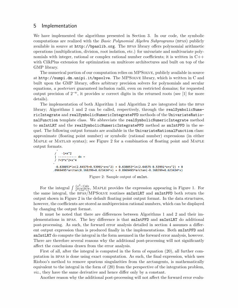
nalFunction template class. We abbreviate the realSymbolicNumericIntegrate methodto snIntLRT and the realSymbolicNumericIntegratePFD method as snIntPFD in the se-quel. The following output formats are available in the UnivariateRationalFunction class:approximate (floating point number) or symbolic (rational number) expressions (in eitherMaple or Matlab syntax); see Figure 2 for a combination of floating point and Mapleoutput formats.
Figure 2: Sample output of snInt.
For the integral ∫(x2−1)dxx4+5x2+7
, Maple provides the expression appearing in Figure 1. Forthe same integral, the bpas/MPSolve routines snIntLRT and snIntPFD both return theoutput shown in Figure 2 in the default floating point output format. In the data structures,however, the coefficients are stored as multiprecision rational numbers, which can be displayedby changing the output format.
It must be noted that there are differences between Algorithms 1 and 2 and their im-plementations in bpas. The key difference is that snIntPFD and snIntLRT do additionalpost-processing. As such, the forward error analysis detailed in section 4 assumes a differ-ent output expression than is produced finally in the implementations. Both snIntPFD andsnIntLRT do compute the integral in the form assumed in the forward error analysis, however.There are therefore several reasons why the additional post-processing will not significantlyaffect the conclusions drawn from the error analysis.
First of all, after the integral is computed in the form of equation (20), all further com-putation in bpas is done using exact computation. As such, the final expression, which usesRioboo’s method to remove spurious singularities from the arctangents, is mathematicallyequivalent to the integral in the form of (20) from the perspective of the integration problem,viz., they have the same derivative and hence differ only by a constant.
Another reason why the additional post-processing will not affect the forward error evalu-
ation is that converting two-argument arctangent functions of polynomials (or one-argumentarctangents of rational functions) to one-arguments arctangents of polynomials increasestheir numerical stability. This is because the derivative of arctan(x) is 1/(1 + x2), whichcan never be zero, or even small, for real integrals, whereas the derivative of arctan(x1, x2)
and arctan(x1/x2) is (x′1x2 − x1x′2)/(x
21 + x
22), which can approach zero for nearly real roots
of the denominator of the integrand. This changes the denominators of the expressions forΘ(rk, sk, x) appearing in the proof of theorem 2. Thus, the application of Rioboo’s methodimproves the stability of the integral. As such, the worst that can happen in this situation isthat the forward error looks to become large when it is not. Though this issue will need tobe resolved in refinements of the implementation, it is very unlikely to be a significant issueon account of the fact that the error is dominated by the error in the roots, and in practicethis error is many orders of magnitude less than the tolerance.
Since the forward error analysis is reliable, modulo the issue just stated, even thoughwe could compute the forward error on the final output, it is a design decision not to doso. This is because a design goal of the algorithm is to hide the error analysis in the maincomputation of the integral by performing the error analysis in parallel. This is only possibleif the error analysis can proceed on information available before the integral computation iscompleted.
6 Experimentation
We now consider the performance of Algorithms 1 and 2 based on their implementations inbpas. For the purposes of comparing their runtime performance we will consider integrationof the following functions:
1. f1(x) =1
xn−2 ;
2. f2(x) =1
xn+x−2 ;
3. f3(x) = [n,n]ex/x(x),
where [m,n]f(x) denotes the Pade approximant of order [m/n] of f . Since ∫ex
x dx = Ei(x),the non-elementary exponential integral, integrating f3 provides a way of approximatingEi(x). These three problems test different features of the integrator on account of the factthat f1(x) has a high degree of symmetry, while f2(x) breaks this symmetry, and f3(x)contains very large integer coefficients for moderate size n. Note that unless otherwise stated,we are running snIntPFD and snIntLRT with the error analysis computation turned on.
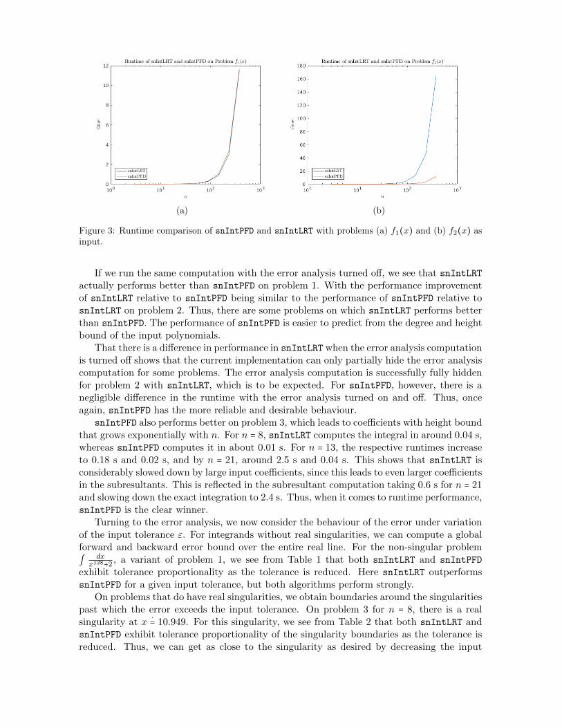
Comparing snIntPFD and snIntLRT on functions f1 and f2 for fibonacci values of n,from n = 3 to n = 377, we find the results shown in Figure 3. We see from Figure 3athat the performance of the two algorithms is nearly identical on function f1(x). Figure3b shows, however, that on function f2(x), snIntPFD performs considerably poorer thansnIntLRT. The reason for this is that the size of the coefficients in the Rothstein-Tragerresultant grows exponentially for f2(x). This causes no significant issues for the subresultantcomputation, but it significantly slows the rootfinding algorithm, leading to large rationalnumber roots, which slows the post-processing algorithms. In contrast, the difference inruntime for snIntPFD on functions f1(x) and f2(x) is negligible. This is because the speed ofsnIntPFD is determined by the degree of the denominator (after the squarefree part has beenextracted by Hermite reduction) and the height of the coefficients. Since the denominators off1 and f2 have the same degree and height bound, we expect the performance to be similar.
(a) (b)
Figure 3: Runtime comparison of snIntPFD and snIntLRT with problems (a) f1(x) and (b) f2(x) asinput.
If we run the same computation with the error analysis turned off, we see that snIntLRTactually performs better than snIntPFD on problem 1. With the performance improvementof snIntLRT relative to snIntPFD being similar to the performance of snIntPFD relative tosnIntLRT on problem 2. Thus, there are some problems on which snIntLRT performs betterthan snIntPFD. The performance of snIntPFD is easier to predict from the degree and heightbound of the input polynomials.
That there is a difference in performance in snIntLRT when the error analysis computationis turned off shows that the current implementation can only partially hide the error analysiscomputation for some problems. The error analysis computation is successfully fully hiddenfor problem 2 with snIntLRT, which is to be expected. For snIntPFD, however, there is anegligible difference in the runtime with the error analysis turned on and off. Thus, onceagain, snIntPFD has the more reliable and desirable behaviour.
snIntPFD also performs better on problem 3, which leads to coefficients with height boundthat grows exponentially with n. For n = 8, snIntLRT computes the integral in around 0.04 s,whereas snIntPFD computes it in about 0.01 s. For n = 13, the respective runtimes increaseto 0.18 s and 0.02 s, and by n = 21, around 2.5 s and 0.04 s. This shows that snIntLRT isconsiderably slowed down by large input coefficients, since this leads to even larger coefficientsin the subresultants. This is reflected in the subresultant computation taking 0.6 s for n = 21and slowing down the exact integration to 2.4 s. Thus, when it comes to runtime performance,snIntPFD is the clear winner.
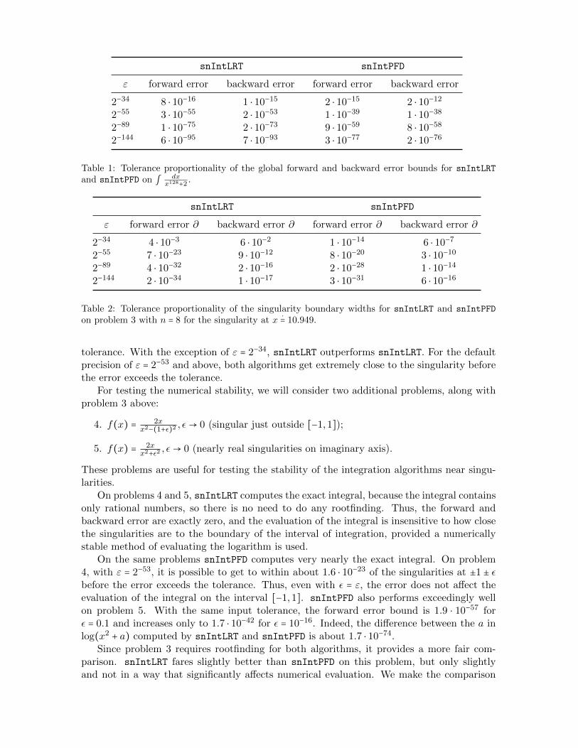
Turning to the error analysis, we now consider the behaviour of the error under variationof the input tolerance ε. For integrands without real singularities, we can compute a globalforward and backward error bound over the entire real line. For the non-singular problem
∫dx
x128+2, a variant of problem 1, we see from Table 1 that both snIntLRT and snIntPFD
exhibit tolerance proportionality as the tolerance is reduced. Here snIntLRT outperformssnIntPFD for a given input tolerance, but both algorithms perform strongly.
On problems that do have real singularities, we obtain boundaries around the singularitiespast which the error exceeds the input tolerance. On problem 3 for n = 8, there is a realsingularity at x
⋅= 10.949. For this singularity, we see from Table 2 that both snIntLRT and
snIntPFD exhibit tolerance proportionality of the singularity boundaries as the tolerance isreduced. Thus, we can get as close to the singularity as desired by decreasing the input
Table 2: Tolerance proportionality of the singularity boundary widths for snIntLRT and snIntPFD
on problem 3 with n = 8 for the singularity at x⋅
= 10.949.
tolerance. With the exception of ε = 2−34, snIntLRT outperforms snIntLRT. For the defaultprecision of ε = 2−53 and above, both algorithms get extremely close to the singularity beforethe error exceeds the tolerance.
For testing the numerical stability, we will consider two additional problems, along withproblem 3 above:
4. f(x) = 2xx2−(1+ε)2
, ε→ 0 (singular just outside [−1,1]);
5. f(x) = 2xx2+ε2
, ε→ 0 (nearly real singularities on imaginary axis).
These problems are useful for testing the stability of the integration algorithms near singu-larities.
On problems 4 and 5, snIntLRT computes the exact integral, because the integral containsonly rational numbers, so there is no need to do any rootfinding. Thus, the forward andbackward error are exactly zero, and the evaluation of the integral is insensitive to how closethe singularities are to the boundary of the interval of integration, provided a numericallystable method of evaluating the logarithm is used.
On the same problems snIntPFD computes very nearly the exact integral. On problem4, with ε = 2−53, it is possible to get to within about 1.6 ⋅ 10−23 of the singularities at ±1 ± εbefore the error exceeds the tolerance. Thus, even with ε = ε, the error does not affect theevaluation of the integral on the interval [−1,1]. snIntPFD also performs exceedingly wellon problem 5. With the same input tolerance, the forward error bound is 1.9 ⋅ 10−57 forε = 0.1 and increases only to 1.7 ⋅ 10−42 for ε = 10−16. Indeed, the difference between the a inlog(x2 + a) computed by snIntLRT and snIntPFD is about 1.7 ⋅ 10−74.
Since problem 3 requires rootfinding for both algorithms, it provides a more fair com-parison. snIntLRT fares slightly better than snIntPFD on this problem, but only slightlyand not in a way that significantly affects numerical evaluation. We make the comparison
for ε = 2−53. With n = 8, for snIntLRT the backward and forward error bounds away fromthe real singularities are about 2.1 ⋅ 10−38 and 1.8 ⋅ 10−36, respectively. For snIntPFD thebackward error bound increases only to 2.6 ⋅ 10−35 and the forward error bound decreasesslightly to 1.2 ⋅ 10−36. As for evaluation near the real singularities, snIntLRT can get withinabout 1.8 ⋅ 10−23 of the singularity at around x = 10.949 before the forward error exceeds thetolerance. snIntPFD can get within about 2 ⋅ 10−20. Of course, this is not a true concernanyway, because the Pade approximant breaks down before reaching the real root.
We see, therefore, that snIntPFD performs strongly against snIntLRT even when snIntLRT
gets the exact answer and snIntPFD does not. Indeed, the differences in numerical stabilitybetween the two methods are very small. Given the performance benefits of snIntPFD, thePFD-based algorithm is the clear overall winner between the two algorithms. Except in caseswhere the exact integral needs to be retained, then, snIntPFD is the preferred choice.
7 Conclusion
We have identified two methods for the hybrid symbolic-numeric integration of rational func-tions on exact input that adjust the forward and backward error the integration according toa user-specified tolerance, determining the intervals of integration on which the integrationis numerically stable. The PFD-based method is overall the better algorithm, being betteroverall in terms of runtime performance while maintaining excellent numerical stability. TheLRT-based method is still advantagous in contexts where the exact integral needs to be re-tained for further symbolic computation. We believe these algorithms, and the extension ofthis approach to wider classes of integrands, has potential to increase the utility of symboliccomputation in scientific computing.
References
[1] Dario A Bini and Leonardo Robol. Solving secular and polynomial equations: A multi-precision algorithm. Journal of Computational and Applied Mathematics, 272:276–292,2014.
[2] Manuel Bronstein. Symbolic integration, volume 3. Springer, 1997.
[3] Manuel Bronstein. Symbolic integration tutorial. https://www-sop.inria.fr/cafe/
[7] William M Kahan. Handheld calculator evaluates integrals. Hewlett-Packard Journal,31(8):23–32, 1980.
[8] Matu-Tarow Noda and Eiichi Miyahiro. On the symbolic/numeric hybrid integration.In Proceedings of the international symposium on Symbolic and algebraic computation,page 304. ACM, 1990.
[9] Matu-Tarow Noda and Eiichi Miyahiro. A hybrid approach for the integration of arational function. Journal of computational and applied mathematics, 40(3):259–268,1992.
[10] Renaud Rioboo. Real algebraic closure of an ordered field: Implementation in Axiom.In Paul S. Wang, editor, Proceedings of the 1992 International Symposium on Symbolicand Algebraic Computation, ISSAC ’92, Berkeley, CA, USA, July 27-29, 1992, pages206–215. ACM, 1992.
[11] Renaud Rioboo. Towards faster real algebraic numbers. J. Symb. Comput., 36(3-4):513–533, 2003.
[12] Zhonggang Zeng. Apatools: a software toolbox for approximate polynomial algebra. InSoftware for Algebraic Geometry, pages 149–167. Springer, 2008.


![arXiv:1201.1548v1 [cs.CG] 7 Jan 2012 - workasm.github.io · Exact Symbolic-Numeric Computation of Planar Algebraic Curves EricBerberich,PavelEmeliyanenko,AlexanderKobel,MichaelSagraloff](https://static.documents.pub/doc/80x56/5e1598d289c08477e81c44c0/arxiv12011548v1-cscg-7-jan-2012-exact-symbolic-numeric-computation-of-planar.jpg)


