Symbolic State-space Exploration and Numerical Analysis of ...

NUMERICAL SOLUTION of MARKOV CHAINS, p. 167–189

Symbolic State-space Exploration and Numerical Analysis ofState-sharing Composed Models

∗ Salem Derisavi1, Peter Kemper2, William H. Sanders1

1 University of Illinois at Urbana-Champaign, Coordinated Science Laboratory, Urbana, IL 61801, USA,{derisavi,whs}@crhc.uiuc.edu

2 Informatik IV, Universitat Dortmund, D-44221 Dortmund, Germany, [email protected]

key words: Multi-valued Decision Diagrams, Matrix Diagrams, Numerical Analysis, Symbolic

State-space Exploration

ABSTRACT

The complexity of stochastic models of real-world systems is usually managed by abstracting details

and structuring models in a hierarchical manner. Systems are often built by replicating and joining

subsystems, making possible the creation of a model structure that yields lumpable state spaces. This

fact has been exploited to facilitate model-based numerical analysis. Likewise, recent results on model

construction suggest that decision diagrams can be used to compactly represent large Continuous Time

Markov Chains (CTMCs). In this paper, we present an approach that combines and extends these

two approaches. In particular, we propose methods that apply to hierarchically structured models

with hierarchies based on sharing state variables. The hierarchy is constructed in a way that exposes

structural symmetries in the constructed model, thus facilitating lumping. In addition, the methods

allow one to derive a symbolic representation of the associated CTMC directly from the given model

without the need to compute and store the overall state space or CTMC explicitly. The resulting

representation of a generator matrix allows the analysis of large CTMCs in lumped form. The efficiency

of the approach is demonstrated with the help of two example models.

1. Introduction

Model-based evaluation of computer and communication systems often takes place bysimulation. In many cases, the desired results could, in principle, also be derived through

∗Correspondence to: 1 University of Illinois at Urbana-Champaign, Coordinated Science Laboratory, Urbana,IL 61801, USA, [email protected]

Contract/grant sponsor: This material is based upon work supported by the National Science Foundation underGrant Nos. CCR-00-86096 and INT-0233490 and by DFG, SFB 559, and the DAAD/NSF exchange project(PPP USA), No. D/0247256. Any opinions, findings, and conclusions or recommendations expressed in thismaterial are those of the authors and do not necessarily reflect the views of the sponsors.

168 S. DERISAVI, P. KEMPER, AND W. H. SANDERS

analysis of generated CTMCs; however, in practice, the size of the systems of equations thatwould need to be solved is prohibitive. This “largeness problem” has motivated much researchin the construction and numerical solution of CTMCs.

Many construction and solution techniques that have been developed for large CTMCscan be classified as “largeness avoidance” techniques in which certain properties of somerepresentation of the model (ranging from the high-level description of the model to theunderlying CTMC itself) are exploited to reduce the size (in number of states and transitions)of the underlying CTMC that needs to be solved to obtain a solution of the model. Forexample, state lumping is an approach that reduces the size of a CTMC by considering thequotient of the CTMC with respect to an equivalence relation that preserves the Markovproperty and many performance measures defined on the CTMC. Since the computation ofthat equivalence relation for a large CTMC is costly in space and time, most practical lumpingapproaches identify appropriate lumpings by operating on a higher-level formalism, rather thanby constructing the unlumped CTMC and then operating on it. For some modeling formalisms,the equivalence that is used for lumping is established by the modeling formalism itself; forinstance, this is the case for stochastic well-formed nets (SWNs) [5] and stochastic activitynetwork-based composed models (SANs) [20]. It can also be shown that lumping has theproperty of a congruence that is preserved by parallel composition in a number of processalgebra formalisms and stochastic automata, so approaches that make use of a compositionalstructure in stochastic process algebras can also be used to generate lumped overall statespaces (e.g., [2]).

Nevertheless, even a lumped state space can be extremely large, and further work on“largeness tolerance” techniques is needed to practically support such lumped state spaces. Forexample, binary and multi-valued decision diagrams (BDDs and MDDs) have been successfullyapplied to explore and represent large unlumped state spaces. The key idea is to encode statesas paths in a directed acyclic graph. Techniques that generate state spaces using decisiondiagrams are referred to as symbolic state-space exploration and representation techniques (e.g.,[10]), and in some cases, they allow one to verify logical properties of systems with “1020 statesand beyond” [4].

For the numerical analysis of CTMCs, it is also necessary to represent the generator matrixQ in a space-efficient manner. Different approaches exist, and one possibility is to follow adivide-and-conquer strategy and represent the overall matrix Q by a set of relatively smallcomponent matrices that are appropriately combined. Such so-called Kronecker representationsare built upon a specific matrix algebra whose operators (Kronecker product and sum) serveas composition operators to build Q from component matrices (e.g., [3, 18, 22]). In thoseapproaches, the composition of a system from subsystems is built upon synchronization ofactions, under certain assumptions about the structure of a model. Alternatively, componentmatrices can be combined using a suitable variant of a decision diagram, namely a matrixdiagram (MD) (e.g., [7, 8, 9, 17]). MDs have been proposed for systems that again are builtin a compositional manner upon synchronization of actions. Another approach is to employmulti-terminal binary decision diagrams (MTBDDs) that store Q(s, s′) at the end of a paththrough a BDD, where the path itself encodes the transition (s, s′) (e.g., [13]). MTBDDs donot rely on a given structure of a model, but they only perform well if there are not toomany different entries in Q(s, s′). Preliminary work on combining state-sharing and actionsynchronization between models for MTBDD-based analysis is reported in [15].

An important result of this paper is that it extends previous work on MDDs and MDs to

SYMBOLIC STATE-SPACE EXPLORATION AND NUMERICAL ANALYSIS OF ... 169

composed models that share state variables and that support next-state and weight functionsthat are state-dependent in general†. Furthermore, it combines lumping techniques, whichhave been applied to state-sharing composed models, with largeness tolerance techniquesthat use MDDs and MDs. In particular, our efforts have resulted in a new algorithm thatsymbolically generates the state space of a hierarchical model (which is built using join andreplicate operators [20]) in the form of an MDD data structure. The replicate operator imposessymmetries that create regular structures in the state space, and therefore make symbolicexploration of the state space efficient with MDDs.

We also designed an algorithm to obtain an MDD representation of the lumped state spacefrom the MDD generated by the state-space generation algorithm. The lumping algorithm,which reduces the size of the state space, also reduces the regularity of the MDD, whoserepresentation becomes larger as a result. However, that increase is negligible compared tothe space used for an iteration vector in the subsequent numerical analysis of the lumpedCTMC. We obtain an MD representation of the lumped CTMC as a projection of the MD ofthe unlumped CTMC on the lumped state space. In performing a numerical analysis on thatMD, one must use extra care in matching states with their corresponding lumped states in thelumped CTMC.

The remainder of the paper is organized as follows. First, we begin in Section 2 with somedefinitions and notations we need to specify the modeling formalism we use and to describeMDDs and MDs. Then, in Section 3, we present a symbolic state-space exploration algorithm.Section 4 discusses how to obtain an MD for the generator matrix of the lumped CTMC andhow to operate on that structure for numerical analysis. The proposed approach has beenimplemented and used for the numerical state-space analysis of a highly redundant fault-tolerant parallel computer system [16, 19]. We also consider a well-known performance modelof a communication protocol [23]. Results for these models are presented in Section 5. Weconclude in Section 6.

2. Background

2.1. Hierarchical Model Specification

In this paper, we develop a representation of the CTMC of a hierarchical composed modelthat is built on shared state variables (SVs) among submodels. This composition operationis the same as the one used in SAN-based reward models [20], but is different from action-synchronization composition, which has been used in superposed generalized stochastic Petrinets, (stochastic) process algebras, and stochastic automata networks. In order to describeprecisely how hierarchical composed models of discrete event systems are constructed, westart with the definition of a model and the composition operators that we use to build thosemodels. Note that the actual formalism used to describe the models we compose together cantake many forms, including stochastic extensions to Petri nets, stochastic process algebras, and“buckets and balls” models, among others. Our intent is not to create yet another formalism,but simply to specify a simple model type that allows us to describe our technique. In reality,

†Approaches based on action synchronization typically impose restrictions on actions that are synchronized.


it will work with any discrete-event formalism that has the characteristics described below,including composed models with constituent models expressed in different formalisms.

Definition 1. A model M is an 8-tuple (V, Vs, Vs, A, s0, δ, w, p) where V is a finite, non-emptyset of SVs and Vs ⊆ Vs ⊆ V . Vs is a set of shared SVs; Vs is a set of exported shared SVs.Dv is the set of possible values v ∈ V can take. A is a finite, non-empty set of actions.A state s is an element of ×v∈V Dv, and s0 is the initial state. The next state functionδ : A× (×v∈V Dv)→ (×v∈V Dv) is only partially defined and describes a successor state fora given action and state. Function w : A × (×v∈V Dv) → IR+ defines a non-negative weightfor an action and p : A→ {0, 1, . . . , n} defines a priority for an action using a finite subset ofIN. For ease of notation, δ(a, s) and w(a, s) are denoted by δa(s) and wa(s), respectively.

Note that we do not impose restrictions on δ and w, as is typically done for formalisms usingaction synchronization. For instance, action synchronization requires that enabling conditionsand state changes of synchronized actions be conjunctions of local conditions and local effects,e.g., the requirement called “product-form” decomposition in [9]. Since we compose models bysharing variables, we can allow δa(s) to be defined in a non-decomposable, rather arbitrarymanner; e.g., δa(s) may be defined only for states where

∑v∈V sv ≥ c, for some constant c. We

compose models by sharing SVs. There are two ways to do so. If M itself consists of submodelsand results from some composition of those submodels (composition operators will be definedbelow) then Vs contains SVs that are shared among those submodels. In addition, if M issubject to composition itself, then certain SVs of M may be shared with other models; set Vs

identifies those externally shared SVs within Vs. The usefulness of subsets Vs and Vs of Vs willbecome more clear after composition operators are defined below.

We will limit ourselves to consideration of models whose behaviors are Markov processes byenforcing the following two restrictions. 1) For any state s and action a with p(a) < n, δa(s)can only be defined if there is no action a′ such that δa′(s) is defined and p(a′) > p(a). If δa(s)is defined, we say that a is enabled in s. 2) If p(a) > 0, then a is called immediate and actiona takes place (fires) with probability wa(s)/

∑a′∈E(s) wa′(s), where E(s) ⊆ A denotes the set

of actions that are enabled in s. If p(a) = 0, then a is timed and action a takes place aftera delay that is exponentially distributed with rate wa(s). Note that δ induces a reachabilityrelation among states and that the reflexive, transitive closure of δ results in the state space ofM . We restrict ourselves to models with a finite state space and those whose structure allowsus to perform an on-the-fly elimination of vanishing states. The resulting set of tangible statesis denoted by S. The generator matrix of the associated CTMC is Q = R−D where R(s, s′)gives the sum of rates of all timed actions whose firing leads from s to s′ (possibly including asubsequent sequence of immediate actions whose probabilities are multiplied with the rate ofthe initial timed action). D = diag(rowsum(R)) provides diagonal entries of Q as the sum ofrow entries of R. In representing Q, we will focus mainly on construction of R, since for anygiven R, derivation of D is straightforward.

In order to build models of complete systems from smaller and simpler models, we definetwo composition operators, “join” and “replicate,” which are based on sharing SVs of themodels on which they are defined [20]. The join operator combines a number of (possiblynon-identical) models by sharing a subset of their SVs, while the replicate operator combinesa number of copies of the same model by sharing the same subset of each of the models’ SVs.The definition of join uses the notion of substate sW , the projection of s on a set of state


variables W ⊆ V .

Definition 2. The join operator J (VJ , M1, . . . , Mn) over models Mi = (Vi, Vsi, Vsi,Ai, s

0,i, δi, wi, pi), i ∈ {1, . . . , n} with VJ ⊆ ∪ni=1Vsi yields a new model M =

(V, Vs, Vs, A, s0, δ, w, p) with state variables V = ∪ni=1Vsi ∪ �n

i=1Vi\Vsi, where an appropriaterenaming of SVs in Vi\Vsi ensures unique names such that the union is over disjoint sets,and where ∪n

i=1Vsi means that SVs with the same names are indeed joined. Vs = ∪ni=1Vsi and

Vs = VJ . A = �ni=1Ai where an appropriate renaming of actions in A1, . . . , An ensures that the

union is over disjoint sets. s0(v) = s0,i(v) if v ∈ Vi − Vsi and s0(v) = maxis0,i(v) if v ∈ Vs.

Functions δ, w, and p are defined such that δa(s) = s′, wa(s) = λ, and p(a) = pi(a) if thereexists i ∈ {1, . . . , n} such that a ∈ Ai, δi,a(sVi) = s′Vi

, wi,a(sVi) = λ, and sV −Vi = s′V −Vi. We

call M1, . . . , Mn the children of model M .

We now more precisely identify the role of Vs and Vs in M . Elements of Vs are SVs sharedamong the children of M , i.e., if Mi and Mj both have an SV x, and if x ∈ Vs, then M containsa single SV x shared by Mi and Mj . On the other hand, if x �∈ Vs then x is renamed in Mi

and Mj (e.g., as xi and xj) such that M contains two different SVs. Furthermore, if M itself isused as a child in a subsequent join operator, only the SVs in Vs are visible and can be sharedwith other children of that join operator.

By convention, we use the maximum initial value of the shared SVs as the value of theresulting shared SV. Note that the join operator is a commutative operator.

Definition 3. The replicate operator Rn(VJ , M) yields a new model M ′ = J (VJ , M1,. . . , Mn) with Mi = M for all i ∈ {1, . . . , n} and VJ ⊆ VsM . We call M the child of modelM ′, and n the cardinality of the operator.

The replicate operator is a special case of the join operator, in which all composed modelsare identical; for that reason, it exhibits desirable properties with respect to the lumpabilityof the CTMC its resulting model generates.

Note that the set of models is closed under the join and replicate operators, meaning thatthe result of each of the operators is a model itself, and therefore can be a child of another joinor replicate operator. This property enables us to build composed models that are hierarchical.Such composed models require a starting set of “atomic” models that act as building blocks.Atomic models are built without use of replicate or join operators and have Vs = Vs since thereis no reason to have shared SVs that are not externally visible. For analysis of a single atomicmodel as such, classical CTMC analysis applies. Hence, in the following, we are interested onlyin composed models that contain at least one join or replicate operator.

For a composed model that is given in terms of possibly nested join and/or replicateoperators, we call each occurrence of an atomic model or the result of each occurrence ofan operator a component. Note that every component is a model. For a model that containsm components we can define an index 1, 2, . . . , m over the components of a term from left toright after expanding replicate operators into join operators. For example,

M = R2(VJ′,J (VJ , M ′, M ′′)) = J (V ′

J ,J (VJ , M ′, M ′′),J (VJ , M ′, M ′′))

obtains indices as in= J1(V ′

J ,J2(VJ , M3, M4),J5(VJ , M6, M7))

where m = 7, the leftmost join operator corresponds to the component with index 1, the secondleftmost join operator has index 2, and the last component is M ′′ to the right with index 7.


Obviously, VJ and V ′J do not receive indices, because they are not components. In the rest of

the paper, the set of SVs of component c, the set of actions of component c, and the set of SVsof model M are respectively denoted by Vc (Vsc, Vsc), Ac, and V . In the following, we consideronly the non-trivial case m > 1. The motivation for this indexing scheme is partitioning of theset of SVs V into m disjoint subsets as follows. If component c corresponds to a join operator,then Vc = Vsc\VJc. If component c is an atomic model, then Vc = Vc\Vsc. The partition isdenoted by P = {V1, . . . ,Vm}, and we call Vi’s (1 ≤ i ≤ m) the blocks of P . ‡

For any component c, we can define an injective mapping gc :×v∈VcDv → IN0 (IN0 is the

set of non-negative integers) that gives an index number to any setting of SVs in Vc. Since weconsider only models with finite state spaces, the domain of gc is finite. Clearly, many suchmappings exist. At this point the only condition on the mapping is that it be injective suchthat any state s = (s1, . . . , sm) ∈ ×m

c=1(×v∈VcDv) of a model, where si = sVi , has a unique

representation as a vector v = (g1(s1), . . . , gm(sm)) in INm0 . The ith component of the vector

v, which is denoted by vi (1 ≤ i ≤ m), is in fact the index of substate sVi . We will use v ands interchangeably to represent states. In that way, we will obtain a uniform representation ofa state as a vector of natural numbers.

An important property of the replicate operator is that it generates a behavior that enableslumping on the associated CTMC of a model [20]. We can define the lumped state space ofa model with full state space S through the help of equivalence relations. In particular, forRnc(VJ , M) with index c and cardinality nc, let lc be the number of indices used for a singlereplica of M . Then, by construction, all indices in the range c, c+1, . . . , c+nclc are associatedwith that replicate component. Let v(c, i) = (vc+ilc+1, . . . , vc+ilc+lc) be a subvector of v ∈ INm

0

for i ∈ {0, . . . , nc − 1}. If the child of a replicate component c is an atomic component, thenlc = 1, and v(c, i) consists of a single element. We define an equivalence relation Rc on v ∈ INm

0

as follows. A pair (v, v′) ∈ Rc with vectors v, v′ ∈ INm0 if and only if

1. vi = v′i for all i ∈ {1, . . . , c, c + nclc + 1, . . . , m} and2. there exists a permutation (a bijective function) q : {0, . . . , nc − 1} → {0, . . . , nc − 1},

such that v(c, i) = v′(c, q(i)) for all i = 0, . . . , nc − 1.

When a hierarchical model contains a number of replicate components, we define the overallequivalence relation R to be the union of equivalence relations over all replicate components,i.e., R = ∪c is replicateRc. In the next section, we describe how we lump the state space S bybuilding the quotient S/R; we identify each equivalence class of R by a specific representativestate. The set of these representative states constitutes the lumped state space, Slumped.

2.2. Review of MDD and MD data structures

In order to compute performance measures of a composed model, we need to construct a CTMCrepresenting the behavior of the model. Our main goal is to extend the size of composed modelsthat can be handled on a typical computer system by using the structural properties of a modelboth to reduce the number of states that need to be considered and to compactly represent

‡Depending on the composed model, some of the blocks of P may be empty. For the sake of simplicity of thepresentation, we assume that all blocks are non-empty. However, the degenerate cases are addressed in ourimplementation.


the states that need to be considered. With that aim, we chose to use MDD and MD datastructures, respectively, to represent the set of states and the set of transitions of the CTMCassociated with a composed model, and use the structural characteristics of the model to lumpequivalent states. In the following, we give a brief description of the two data structures.

Multi-valued Decision Diagrams Review. MDDs [21] generalize binary decisiondiagrams (BDDs) [1]. They are useful for encoding a set of vectors S ⊆ ×m

i=1 Si since theycan represent functions of the form f :×m

i=1 Si → {0, 1} for finite sets Si = {0, . . . , |Si| − 1},i = 1, . . . , m. Hence, (s1, . . . , sm) is an element of S if and only if f(s1, . . . , sm) = 1. MDDsare ordered, i.e., the order of Si’s is fixed; we consider the order S1, . . . , Sm. They are rooted,directed, acyclic graphs (“folded trees”) with terminal and non-terminal nodes. A terminalnode is either 0 or 1; a non-terminal node has a variable xi ∈ Si assigned to it and contains|Si| pointers to a node with a variable xj , j > i or to a terminal node. A pointer correspondsto a co-factor of f that is defined as fxi=c = f(s1, . . . , si−1, c, si+1, . . . , sm) for variable xi anda constant c ∈ Si. Since the order is fixed, a node with variable xi is referred to as a level-inode, and the function that a level-i node represents is denoted by (xi, fxi=0, . . . , fxi=|Si|−1).In the algorithms we develop, we use u[k] to denote the node to which the kth pointer ofa non-terminal node u points, and the set of all level-i nodes is denoted by Ni. u[k] is alsocalled a child of node u. As described in [9], typical set operations like union, intersection, anddifference can be performed on MDDs efficiently. MDDs are often enhanced by a so-called offsetfunction ρ : S → {0, 1, . . . , |S|− 1}, where the ith element of S with respect to lexicographicalorder obtains value i−1. ρ is encoded through assignment of an additional weight ρi(s1, . . . , sk)to each pointer of a level-i node u with value k, and the offset of s is the sum of weights alongthe corresponding path in the MDD, i.e., ρ(s) =

∑mi=1 ρi(s1, . . . , si).

The main advantage of MDDs is that a reduction operation is used to represent isomorphicsubgraphs only once. This reduction is based on a notion of equality for nodes; twonodes are equal if they are terminal nodes of the same value or if they have equal tuples(xi, fxi=0, . . . , fxi=|Si|−1). A non-terminal node is redundant if all of its pointers point to thesame node. We follow [8] and consider ordered MDDs, where equal nodes have been mergedand redundant nodes are retained only to ensure that a pointer of a level-i node can lead onlyto a level-(i + 1) node or to the terminal node with value 0. The value of function f is derivedby following a path in an MDD graph starting at the root node and ending, after at most mnodes, at a leaf node that represents the resulting value of {0, 1}. At each intermediate level-inode, a successor node is selected according to si. MDDs are particularly space-efficient forrepresentation of S when there are a significant number of common subvectors in S. In the restof the paper, the MDD representation of a set (e.g., S) is denoted by the calligraphic letter(e.g., S) corresponding to that set.

Matrix Diagram Review. An MD is a directed acyclic graph like an MDD, but its nodesare matrices; MD provides one matrix per node, whereas an MDD provides one vector per node.However, there are further differences. A non-terminal Si×S′

i matrix at level i ∈ {1, . . . , m} ofan MD contains elements that are sets of pairs. Each pair (r, p) consists of a real value r anda pointer to a level-(i + 1) node or a terminal node. Terminal nodes are 1× 1 matrices withentries {0, 1}. Clearly, only paths that finally lead to the entry 1 are relevant, so terminal nodesare necessary only so that the theoretical framework will be coherent; they are not explicitly


considered in an implementation.As in MDDs, the order of levels is fixed, and we can define two level-i nodes to be equal

if their matrices are equal. Again, we consider a reduced structure in which equal nodes havebeen merged. In a reduced MD, any two pairs (r, p), (r′, p′) in a matrix entry (si, s

′i) of some

level-i node are replaced by a pair (r + r′, p) if p = p′. Let Π denote the set of all paths withelements (si, s

′i, ri, pi) that start at the root node and follow a sequence (s1, s

′1), . . . , (sm, s′m)(1)

of matrix elements (r1, p1), . . . , (rm, pm) that ends at 1. A matrix diagram encodes a functionf : ×m

i=1(Si × S′i) → IR where f((s1, s

′1), . . . , (sm, s′m)) =

∑π∈Π

∏mi=1,(si,s′

i,ri,pi)∈π ri, i.e., realvalues are multiplied along a path and summed over all paths. This definition allows us to useMDs to encode a matrix like R. Algorithms for manipulating MDs are described in detail in[8]. In order to make the MDs that we generate compatible with the MDD of the state space,we encode the SVs in Vi in level i of the MD, as we did for the MDD.

3. Symbolic Generation of Lumped State Space

In this section, we will give a detailed description of our new algorithm for symbolic generationof the lumped state space of a composed model. In doing so, we first describe the state-space generation (SSG) algorithm that does not take lumping properties into account, andtherefore generates the unlumped state space. Then we give an algorithm that exploits thestructural properties of the replicate operator to lump the state space computed by the previousalgorithm.

3.1. Symbolic Generation of Unlumped State Space for Composed Models

A symbolic SSG algorithm is similar to a traditional one in the sense that both algorithmsstart with the initial state of the model and keep firing actions until all reachable states havebeen explored. The difference is that in a traditional algorithm, each time an action is firedonly one state is visited, while in a symbolic algorithm, a (potentially large) set of states isvisited. In our SSG algorithm, we use MDDs to represent sets of states. In order to designan efficient symbolic algorithm for composed models, we identify key structural propertiesof a model, and based on those properties we determine the “meaning,” with respect to thecomposed model structure, of each level of the MDD. In particular, when we use an MDD torepresent the set of states of a model, we represent each state of the model by a vector. Thisvector representation is determined by partition P of the set of SVs. More formally, for eachcomponent 1 ≤ c ≤ m, level c of the MDD represents substates of the form sc. In other words,we define Sc, the set of possible values of a level-c node, such that |Sc| = |{sc|s ∈ S}|.

An action a is called independent of a set of SVs W (in the context of a model M) if a’snext state function δ and weight w are evaluated independently from the value settings forSVs in W ; otherwise, a is dependent on W . To support our SSG algorithm, we partition theset of actions Ac of an atomic component c into Ac,l and Ac,g, which are the sets of local andglobal actions of component c, respectively. a is global if it is dependent on any shared SV,and it is local otherwise. More formally, a ∈ Ac,l if and only if a is independent of Vc\Vc.

In order to design an efficient state-space generation algorithm, we consider a restrictedclass of composed models in which all global actions are of the lowest priority, i.e., they aretimed actions. There are no other restrictions on how actions are enabled or change state, i.e.,


δa(s) can be an arbitrary function on its atomic model’s SVs. This generality implies that adistinction into acylic and cyclic dependencies as discussed in [22] does not apply. There isno restriction on local actions. The slight restriction on global actions we do have has twoimportant implications that enable us to design an efficient SSG algorithm: 1) the eliminationof vanishing states can take place locally, i.e., in each atomic component, and on the fly,i.e., without storing intermediate vanishing states, and 2) atomic components that share SVscannot stop one another from proceeding locally. The latter property gives us the ability touse an approach similar to saturation [6] (in firing local actions) and generate a subset of thestate space of an atomic component independently from other atomic components as long asthe fired actions are independent from the shared SVs of that component, i.e., the actions arelocal.

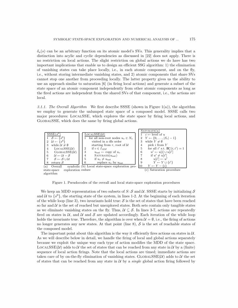
3.1.1. The Overall Algorithm We first describe SSSE (shown in Figure 1(a)), the algorithmwe employ to generate the unlumped state space of a composed model. SSSE calls twomajor procedures: LocalSSE, which explores the state space by firing local actions, andGlobalSSE, which does the same by firing global actions.

SSSE(s0)1 S ← {s0}2 U ← {s0}3 while U �= ∅4 LocalSSE(U)5 GlobalSSE(U)6 U ← U − S7 S ← S ∪ U8 return S

(a) Overall symbolicstate-space explorationalgorithm

LocalSSE(U)1 for all non-root nodes uc ∈ Nc

visited in a dfs orderstarting from r, root of U

2 if c ∈ IAM

3 usat ← copy of uc

4 Saturate(usat)5 if uc �= usat

6 replace uc by usat

(b) Local state-space exploration pro-cedure

Saturate(u)1 c← level of u2 Y ← {0, . . . , |Sc| − 1}3 while Y �= ∅4 pick i from Y5 for all i′ s.t. B∗

c(i, i′) = 16 u′ ← u[i] ∪ u[i′]7 if u′ �= u[i′]8 u[i′]← u′9 Y ← Y ∪ {i′}

10 Y ← Y − {i}(c) Saturation procedure

Figure 1. Pseudocodes of the overall and local state-space exploration procedures

We keep an MDD representation of two subsets of S: S and U . SSSE starts by initializing Sand U to {s0}, the starting state of the system, in lines 1-2. At the beginning of each iterationof the while loop (line 3), two invariants hold true: S is the set of states that have been reachedso far and U is the set of reached but unexplored states. Both sets contain only tangible statesas we eliminate vanishing states on the fly. Thus, U ⊆ S. In lines 3-7, actions are repeatedlyfired on states in U , and U and S are updated accordingly. Each iteration of the while loopholds the invariants true. Therefore, the algorithm is over when U = ∅, i.e., the firing of actionsno longer generates any new states. At that point (line 8), S is the set of reachable states ofthe composed model.

The important point about this algorithm is the way it efficiently fires actions on states in U .As we will describe below in detail, we handle the firing of local and global actions separatelybecause we exploit the unique way each type of action modifies the MDD of the state space.LocalSSE(U) adds to U the set of states that can be reached from any state in U by a (finite)sequence of local action firings. Note that the local actions are timed; immediate actions aretaken care of by on-the-fly elimination of vanishing states. GlobalSSE(U) adds to U the setof states that can be reached from any state in U by a single global action firing followed by


a (finite) sequence of immediate (local) action firings.LocalSSE and GlobalSSE do not take into account the lumping properties of replicate

operators. Instead, they treat replicate operators as join operators with identical children.Moreover, they consider firing actions of atomic components only, because join and replicateoperators do not introduce new actions of their own.

3.1.2. Firing Local Actions By definition, a local action a ∈ Ac,l is independent of Vc\Vc,and therefore δa(s) depends only on sVc . Furthermore, by the restriction we introduced earlier,all immediate transitions are local. Finally, note that all SVs in Vc are encoded in level c ofthe MDD. These properties imply that in order to generate a set of states that are visited bycompletion of action a, we only need to manipulate the nodes in level c of the MDD.

Suppose that a (tangible) substate sc can lead to a tangible substate s′c by a sequenceof actions in Ac,l. Hence, if state (v1, . . . , vc−1, i, vc+1, . . . , vm) is reachable, then state(v1, . . . , vc−1, i

′, vc+1, . . . , vm) is also reachable where i = gc(sc) and i′ = gc(s′c). To implementthis local state exploration on the MDD, we perform the “saturation” operation on all nodesu in level c: u[i′] ← u[i] ∪ u[i′] for all possible values of i and i′. In that operation, valuesof vj ’s are implicit; all state paths that go through u constitute all states of the form(v1, . . . , vc−1, i, vc+1, . . . , vm).

Figure 1(b) shows LocalSSE, which explores the state space using only local actions Ac,l

of every atomic component c. Therefore, LocalSSE iterates through all nodes uc of levelsthat correspond to atomic components (denoted by IAM ) in depth-first search (dfs) order. Foreach node uc, which encodes a set of substates of the form sc, it saturates usat, the node thatis to be the saturated version of uc, by calling Saturate(usat) in line 4. Finally, in lines 5-6,uc is replaced by its saturated version usat.§ The reason for iterating through all nodes in dfsorder is that (due to implementation issues) we need to ensure that a node is saturated afterall its children have been saturated.

Saturate(u) (shown in Figure 1(c)) fires local actions until no further local actionfiring can add any substate to the set. Lines 3-10 perform the abovementioned saturationoperation on u in a “symbolic” manner, i.e., for each i′, lines 6-8 add all states of the form(v1, . . . , vc−1, i

′, vc+1, . . . , vm) to U . Notice that during the saturation operation, we may needto increase the size of u (i.e., the number of its pointers), since we do not know the size of thestate space of Mc in advance. The important point is that due to the locality of the actions,we can expand the set of reachable states of the system only by (local) changes to u.

Repetitive computations related to local state exploration might occur, since the samesubstate may be explored many times for different nodes throughout the execution of SSSE. Inorder to prevent these extra computations, we need an efficient data structure for each atomiccomponent c that stores the reachability relation among substate indices of that component.More formally, we need to know, for every i, the set of all substate indices i′ where substatewith index i′ can be reached from substate with index i′ by a (finite) sequence of local actionfirings. We can determine that by computing the reflexive and transitive closure of a squareBoolean-valued matrix denoted by Bc. Bc is defined on the tangible state space of Mc, which

§In the actual implementation, uc is not replaced by usat in one step. Instead, uc is replaced by usat foreach of the pointers coming from the upper level. Hence, eventually no node will point to uc, uc will begarbage-collected, and therefore uc will essentially be replaced by usat.


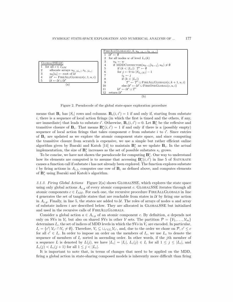
GlobalSSE(U)1 for all c ∈ IAM

2 allocate arrays u0..|Lc|, i0..|Lc|3 u0[i0]← root of U4 U ′ ← FireAllGlobals(c, 1, u, i)5 U ← U ∪ U ′

(a)

FireAllGlobals(c, k, u0..|Lc|, i0..|Lc|)1 U ′ ← ∅2 for all nodes w of level Lc(k)3 uk ← w4 if MDDConnector(uk−1[ik−1], uk) �= ∅5 if (k < |Lc|) T ′ ← ∅6 for j ← 0 to |SLc(k)| − 17 ik ← j8 if (k < |Lc|)9 T ′ ← T ′ ∪ FireAllGlobals(c, k + 1, u, i)

10 else U ′ ← U ′ ∪ FireOneGlobal(c, u, i)11 U ′ ← U ′ ∪ T ′12 return U ′

(b)

Figure 2. Pseudocode of the global state-space exploration procedure

means that Bc has |Sc| rows and columns. Bc(i, i′) = 1 if and only if, starting from substatei, there is a sequence of local action firings (in which the first is timed and the others, if any,are immediate) that leads to substate i′. Otherwise, Bc(i, i′) = 0. Let B∗

c be the reflexive andtransitive closure of Bc. That means B∗

c(i, i′) = 1 if and only if there is a (possibly empty)

sequence of local action firings that takes component c from substate i to i′. Since entriesof Bc are updated as we explore the atomic component state space, and since computingthe transitive closure from scratch is expensive, we use a simple but rather efficient onlinealgorithm given by Ibaraki and Katoh [14] to maintain B∗

c as we update Bc. In the actualimplementation, the size of B∗

c increases as the set of possible substates sc grows.To be concise, we have not shown the pseudocode for computing B∗

c . One way to understandhow its elements are computed is to assume that accessing B∗

c(i, i′) in line 5 of Saturatecauses a function call if substate i has not already been explored. The function explores substatei by firing actions in Ac,l, computes one row of Bc as defined above, and computes elementsof B∗

c using Ibaraki and Katoh’s algorithm.

3.1.3. Firing Global Actions Figure 2(a) shows GlobalSSE, which explores the state spaceusing only global actions Ac,g of every atomic component c. GlobalSSE iterates through allatomic components c ∈ IAM . For each one, the recursive procedure FireAllGlobals in line4 generates the set of tangible states that are reachable from states in U by firing one actionin Ac,g. Finally, in line 5, the states are added to U . The roles of arrays of nodes u and arrayof substate indices i are described below. They are allocated in GlobalSSE but initializedand used in the recursive calls of FireAllGlobals.

Consider a global action a ∈ Ac,g of an atomic component c. By definition, a depends notonly on SVs in Vc but also on shared SVs in other V sets. The partition P = {V1, . . . ,Vm}determines Ic, the set of indices of MDD levels in which the SVs in Vc are encoded. In particular,Ic = {c′| Vc′ ∩ Vc �= ∅}. Therefore, Vc ⊆ ∪c′∈IcVc′ , and, due to the order we chose on P , c′ ≤ cfor all c′ ∈ Ic. In order to impose an order on the members of Ic, we use Lc to denote thesequence of members of Ic sorted in ascending order. In other words, if the jth member ofa sequence L is denoted by L(j), we have |Lc| = |Ic|, Lc(j) ∈ Ic for all 1 ≤ j ≤ |Lc|, andLc(j) < Lc(j + 1) for all 1 ≤ j < |Lc|.

It is important to note that, in terms of changes that need to be applied on the MDD,firing a global action in state-sharing composed models is inherently more difficult than firing


a synchronizing action in an action-synchronization model, as discussed in [6]. The reasonis that in the latter case, the sets of SVs of atomic submodels are disjoint, and due to theproduct-form behavior [6], the changes that need to be applied on a node v (in the levelcorresponding to an atomic model) during saturation depend only on the information presentin v and the action a to be fired, regardless of whether a is local or synchronizing. However,in the former case, some SVs are shared among atomic models, so that firing a global action aon a node v requires not only the information in v but also the information in other levels ofthe MDD. This makes the saturation approach inapplicable in the case of firing global actionsin state-sharing composed models.

Now that we know what levels of the MDD are affected by action a, we discuss how theyare affected. To fire action a, we need to add the state (s′Vc

, sV \Vc) to U for each state s ∈ U

where δa(s) = s′. To realize this state addition operation on the MDD, we have to considerthe paths corresponding to all such states s. Then, for each path, we have to update nodes inappropriate levels. However, considering the paths one by one is not the best way to do so.To describe the better method we have developed, we first need to define the concept of an“MDD connector.” An MDD connector between two nodes w and w′ is a subgraph of the MDDthat includes only sub-paths of the MDD that start from w and end with w′. MDD connectorsconnect the nodes of levels in Ic if they differ by more than one level.

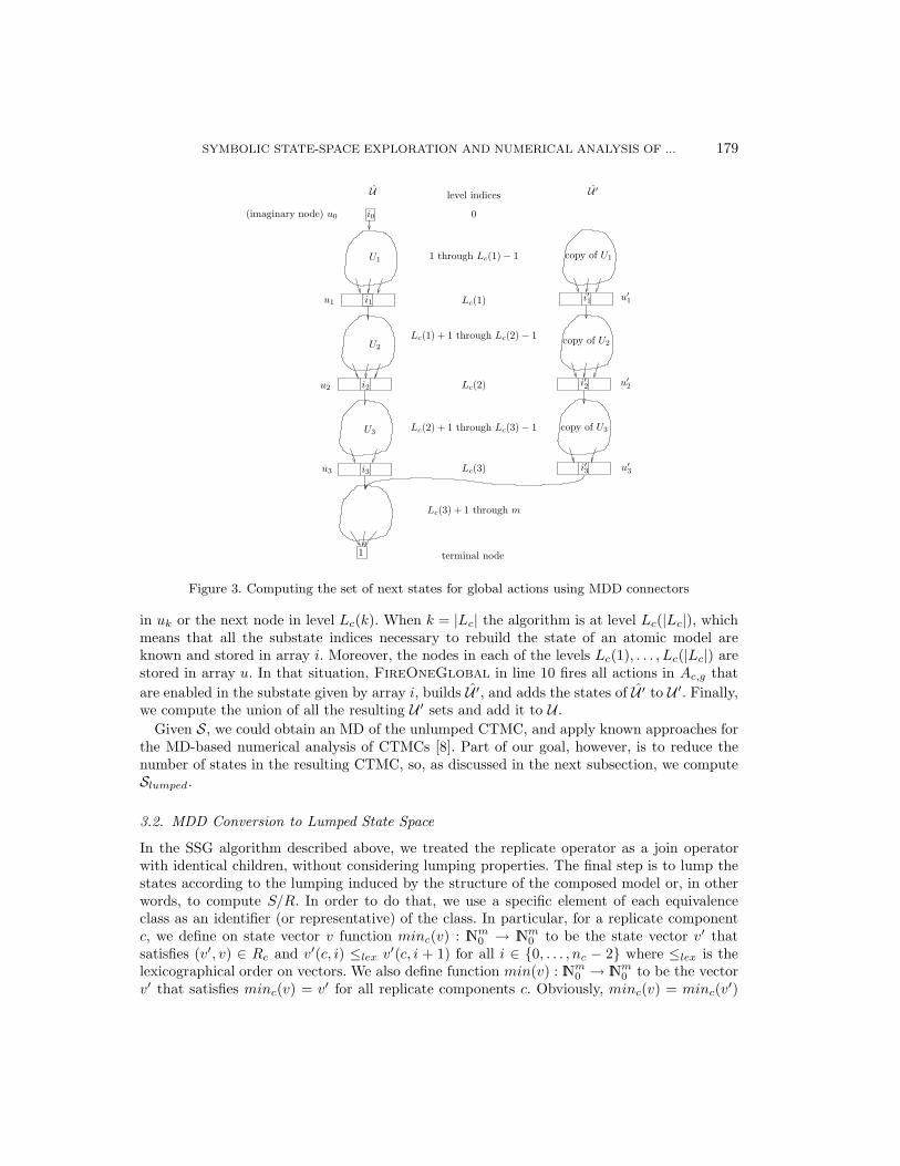
To illustrate this, consider the example in Figure 3, in which |Lc| = 3. u0 is an imaginarynode such that u0[i0] is equal to the root of U¶ (line 3 of GlobalSSE). It is used to avoidcase-by-case analysis, and thus to simplify the presentation. uk is a node in level Lc(k) ofthe MDD for k ∈ {1, . . . , |Lc|}. The left-hand side of the figure shows all paths of the MDD(before firing action a) that pass through all uk’s. Let U be the set of all states that these pathsrepresent. Let Uk be the MDD connector between uk−1[ik−1] and uk where ik = gc(sLc(k)).FireOneGlobal, which is called by FireAllGlobals (Figure 2(b)) generates another MDDthat represents the set of states reachable from U by firing of all actions a ∈ Ac,g, that is,U ′ = {(s′Vc

, sV \Vc)|s ∈ U , δa(s) = s′, a ∈ Ac,g}. Notice that in order to generate U ′, we do not

need to change the nodes in any of the Uk’s (k ∈ {1, . . . , |Lc|}), because action a is independentof the SVs encoded in the levels corresponding to Uk’s. Instead, FireOneGlobal 1) makes acopy of each Uk, 2) computes i′k = gc(s′Lc(k)) and creates new nodes u′

k for each enabled actionin Ac,g, and 3) connects all the new nodes as shown on the right-hand side of Figure 3 in orderto build U ′. Because of limited space, the pseudocode of FireOneGlobal is not given.

To generate states reached by firing actions in Ac,g from all states in U , we have to consider alldistinct sets of nodes {u1, . . . , u|Lc|} (i.e., nodes with index levels in Lc) and their correspondingindices: i1, . . . , i|Lc|. For each of the distinct sets of nodes and indices we have to consider thecorresponding U and generate the corresponding U ′ as described above. Generation of all suchU ′’s is the role of FireAllGlobals(c, k, u0..|Lc|, i0..|Lc|), which recursively iterates through allnodes in the levels Lc(k), . . . , Lc(|Lc|) (line 2) and all substate indices (line 6) of those nodes.In each recursive call, MDDConnector in line 4 checks whether there is an MDD connectorbetween two neighboring nodes, i.e., between uk−1[ik−1] and uk. If there is one, the proceduregoes deeper down in the MDD by a recursive call; otherwise, it tries the next substate index

¶Strictly speaking, no such u0 exists, because there is no node that points to any level-1 node, including theroot of U .


(imaginary node) u0

u1

u2

u3

u′1

u′2

u′3

U1

U2

U3

copy of U1

copy of U2

copy of U3

i0

i1

i2

i3

i′1

i′2

i′3

U U ′

1

0

1 through Lc(1)− 1

Lc(1)

Lc(1) + 1 through Lc(2)− 1

Lc(2)

Lc(2) + 1 through Lc(3)− 1

Lc(3)

Lc(3) + 1 through m

level indices

terminal node

Figure 3. Computing the set of next states for global actions using MDD connectors

in uk or the next node in level Lc(k). When k = |Lc| the algorithm is at level Lc(|Lc|), whichmeans that all the substate indices necessary to rebuild the state of an atomic model areknown and stored in array i. Moreover, the nodes in each of the levels Lc(1), . . . , Lc(|Lc|) arestored in array u. In that situation, FireOneGlobal in line 10 fires all actions in Ac,g thatare enabled in the substate given by array i, builds U ′, and adds the states of U ′ to U ′. Finally,we compute the union of all the resulting U ′ sets and add it to U .

Given S, we could obtain an MD of the unlumped CTMC, and apply known approaches forthe MD-based numerical analysis of CTMCs [8]. Part of our goal, however, is to reduce thenumber of states in the resulting CTMC, so, as discussed in the next subsection, we computeSlumped.

3.2. MDD Conversion to Lumped State Space

In the SSG algorithm described above, we treated the replicate operator as a join operatorwith identical children, without considering lumping properties. The final step is to lump thestates according to the lumping induced by the structure of the composed model or, in otherwords, to compute S/R. In order to do that, we use a specific element of each equivalenceclass as an identifier (or representative) of the class. In particular, for a replicate componentc, we define on state vector v function minc(v) : INm

0 → INm0 to be the state vector v′ that

satisfies (v′, v) ∈ Rc and v′(c, i) ≤lex v′(c, i + 1) for all i ∈ {0, . . . , nc − 2} where ≤lex is thelexicographical order on vectors. We also define function min(v) : INm

0 → INm0 to be the vector

v′ that satisfies minc(v) = v′ for all replicate components c. Obviously, minc(v) = minc(v′)


for all (v, v′) ∈ Rc, and similarly min(v) = min(v′) for all (v, v′) ∈ R. Given any vector v,the corresponding class identifier min(v) can be computed by appropriate sorting operationson v. Notice that for every equivalence class C of S/R there exists only one v such that v ∈ Cand min(v) = v. To compute S/R we eliminate from S all paths (states) that do not satisfymin(v) = v. That computation is translated, in terms of MDDs, to the computation of S ∩R,where R is the MDD representation of the set of all states v ∈ INm

0 that satisfy min(v) = v.Hence, the problem of computing S/R is reduced to building R based on the definition of min.

However, the definition of min(v) imposes a strict relationship among the variouscomponents of vector v, which implies a tight coupling among levels of R in terms of MDDs.That implies that the number of nodes of R grows very quickly in terms of the number oflevels involved in the definition of min(v),‖ and this makes the direct computation of S ∩ Rproblematic.

To avoid this large memory consumption, we can express the large MDD of R in terms ofa small number of considerably smaller MDDs, and instead of computing S ∩ R directly, wecompute the intersection of S with a large set expression that is equal to R. As the first step,we observe that R = ∩c is replicateRc where Rc is the set of all states v ∈ INm

0 that satisfyminc(v) = v. That implies S ∩R = (· · · (S ∩Rc1)∩ · · · ∩Rcj ), where c1, . . . , cj are the indicesof all replicate components of a composed model. Since in general, each of the Rc’s involvestight coupling among far fewer levels than R does, each Rc is significantly smaller than R.Hence, computing (· · · (S ∩ Rc1) ∩ · · · ∩ Rcj ) is much faster than computing S ∩ R directly,because the efficiency we gain by using smaller-sized Rc’s outweighs the extra time we haveto spend to compute j intersection operations rather than one.

Still, we can do better. The next phase is to divide each Rc into many MDDs, each of whichhas tight coupling between only two levels. As an example, suppose lc = 1 for a replicatecomponent c. Then Rc is the MDD representation of the set of vectors v ∈ INm

0 that satisfyvc+1 ≤ . . . ≤ vc+nc , and therefore, Rc involves coupling among nc levels. However, we haveRc = Rc,1∩· · ·∩Rc,nc−1 whereRc,i (1 ≤ i < nc) is the set of vectors that satisfy vc+i ≤ vc+i+1.Now, instead of computing S ∩ Rc directly, we compute (· · · (S ∩ Rc,1) ∩ · · · ∩ Rc,nc−1). Forcases in which lc > 1, the same technique is still applicable, and generally, it can be shownthat indirect computation of S ∩ Rc involves creating O(nclc) small MDDs and performingO(nclc) MDD set operations (i.e., union and intersection), where O is the big O notation.

4. State Transition Rate Matrix Generation and Numerical Analysis

In this section, we describe how to perform an iterative numerical analysis based on an MDrepresentation of R for the lumped CTMC. Its basic step is a matrix-vector multiplication,which requires consideration of several issues if it is performed with an MD. We start withthe generation of an MD from the local transition rate matrices generated during state-spaceexploration. In Section 3 only Boolean matrices Bc of state transitions are mentioned; however,it is straightforward to have corresponding rates (possibly scaled by probabilities of paths

‖In the case of nested replicate operators, we claim that this number can be exponential in terms of thecardinality of the inner replicate operators. Proving this claim is not difficult, but to be concise, we do not givea proof here.


of subsequent immediate transitions) as matrix entries yielding matrices Rc. With the MDrepresentation of the unlumped CTMC at hand, we need to focus on Slumped as the set of rows.Matrix entries in those rows will refer to columns s′ whose correspondence to min(s′) mustbe established. Finally, there are cases in which the MD will generate multiple elements thatmust be added for a single matrix entry in Rlumped. These issues are resolved in the remainingsection.

4.1. State Transition Rate Matrix Generation using MDs

Formally, we first derive a generalized Kronecker representation of the rate matrix R thatgives us an oversized MD in a straightforward manner, and then use the MDD to obtaina projection to the lumped state space. Conceptually, MD generation with the help of aKronecker representation and MDD projection follows the line of arguments in [8]. However,it differs in important aspects. In particular, the Kronecker representation we derive containsfunctional transitions [22] that are subsequently resolved to constant values in the MD. TheMD that finally results requires additional, specific algorithms to describe the rate matrix ofthe lumped CTMC. Note that an implementation directly generates an MD based on the localtransition rate matrices obtained during state-space exploration.

A Kronecker representation for R. A Kronecker structure makes use of the matrixoperator Kronecker product ⊗ to combine small component matrices into a large matrix. Thebuilding blocks of the Kronecker representation are matrices Ra,c that represent the effect oftimed action a on atomic component c.∗∗ Let γc : S → ×v∈VcDv be a mapping that providesthe state in terms of its SVs for an atomic model Mc with component index c. Also letnc = |codomain(γc)|. In fact, Ra,c ∈ IRnc×nc , and Ra,c(s, s′) is the weight of a at s multipliedby the probability of reaching s′ via some sequences of immediate actions in Mc, where s ands′ are states of atomic component c.

Note that the difficulty in the derivation of Ra,c is not in calculating entries, which is doneby using the definition of Mc. The difficulty is in finding the set of reachable states of Mc,since sharing s with other models causes other models to generate new states as well††. Thisdifficulty is overcome by using S as described below. Specifically, for each timed action aand atomic component c, we define m matrices Ri

a,c, i ∈ {1, . . . , m} where Ria,c denotes the

projection of Ra,c on Si × Si and Si = {si|s ∈ S}. In fact, Ria,c denotes the “effect” of Ra,c

on level i of the MD representation of R. More formally, Ria,c ∈ IRSi×Si and

Ria,c(si, s

′i) =

1 if i �= c and ∃s = (s1, . . . , sm), s′ = (s′1, . . . , s′m) ∈ S

such that Ra,c(γc(s), γc(s′)) �= 0fa if i = c and ∃s = (s1, . . . , sm), s′ = (s′1, . . . , s′m) ∈ S

such that Ra,c(γc(s), γc(s′)) �= 00 otherwise

where fa : S × S → IR is a functional transition that evaluates to Ra,c(γc(s), γc(s′)) for given

∗∗Immediate actions are used only during the on-the-fly eliminations of vanishing states.††Formally, one may consider those new states as a set of initial states S0 that may grow as a result of firingglobal actions of other models.


states s, s′; see [22] for the definition and treatment of Kronecker representations that aregeneralized with respect to functions as matrix entries. Notice that Ri

a,c is simply an identitymatrix if i �∈ Ic, where, as defined before, Ic is the set of indices of MDD levels in which theSVs in Vc are encoded.

With those matrices, we obtain a Kronecker representation to describe a state transitionrate matrix R. Its basic operation, the Kronecker product C = A⊗B, is defined for matricesA ∈ IRn×m, B ∈ IRk×l, and C ∈ IRnk×ml as C(a1 · k + b1, a2 · l + b2) = A(a1, a2) ·B(b1, b2). Wedefine R as

R =∑

Mc∈AM

∑a∈Ac

⊗mi=1R

ia,c, (1)

where AM stands for atomic models. We briefly argue why R is a submatrix of R. We consideran entry R((s1, . . . , sm), (s′1, . . . , s

′m)) = λ. Since several actions may contribute to λ we

have λ =∑

a∈E(s) λa(s, s′) where λa(s, s′) is wa(s) possibly multiplied by the probabilityof a subsequent sequence of immediate actions yielding s′. For any term λa(s, s′) > 0, wedefined Ri

a,c(si, s′i) = λi > 0 for i = 1, . . . , m. Since only λc �= 1 we have

∏mi=1 λi = λc =

fa = Ra,c(γc(s), γc(s′)). By the definition of Kronecker product, ⊗mi=1R

ia,c contributes λc =∏m

i=1 Ria,c(si, s

′i) to R((s1, . . . , sm), (s′1, . . . , s

′m)). R is a submatrix of R since S ⊆ ×m

i=1Si.

MD construction for lumped state-transition rate matrix. Transformation of aKronecker representation into an MD is immediate. For each term ⊗m

i=1Ria,c, we define an

MD with 1 node per level, the node at level i contains matrix Ria,c, and its nonzero entries

point to node i+1. In the case of i = m, the nonzero entries formally point to terminal node 1.Since addition is defined for MD, we can sum the resulting MDs of all terms in the two sumsin Eq. 1. Note that the functional transitions that appear in Ri

a,c can be resolved to constantvalues in the MD, because sets Vi are ordered such that the sets that contain shared SVs of anatomic model Mc all have lower indices than c, and thus those sets appear at a higher level ofMD. Hence, if a path through the MD reaches level c, the values of all shared SVs are known.Resolving functional transitions into constant values may require the splitting of matrices thatwere otherwise shared in the MD.

The advantage of an MD over a Kronecker representation is that we can restrict the MDto the S × S submatrix contained in a Kronecker representation. In order to restrict thisrepresentation to S, we refine the definition of matrices as Ri

a,c[(s1, . . . , si−1), (s′1, . . . , s′i−1)] ∈

IRSi×Si for an atomic model at component c and action a to depend on the subset of states(s1, . . . , si−1), (s′1, . . . , s

′i−1), namely:

Ria,c[(s1, . . . , si−1), (s′1, . . . , s′i−1)](si, s

′i)

=

1 if i �= c and ∃s = (s1, . . . , sm), s′ = (s′1, . . . , s′m) ∈ S s.t. Ra,c(γc(s), γc(s′)) �= 0

Ra,c(γ′c(s1, . . . , sc), γ′

c(s′1, . . . , s

′c)) if i = c

0 otherwise

where γ′c is the same as γc but defined on components 1, . . . , c, which is possible since all

(shared) SVs of atomic model Mc appear at components i ≤ c and a is independent ofSVs at components c + 1, . . . , m. That means that for any (s1, . . . , sm) ∈ S the equalityγ′

c(s1, . . . , sc) = γc(s1, . . . , sm) holds. To build a matrix diagram out of these matrices, we let anentry in Ri

a,c[(s1, . . . , si−1), (s′1, . . . , s′i−1)](si, s′i) point to matrix Ri+1

a,c [(s1, . . . , si), (s′1, . . . , s′i)]


if i < m. Pointers from nonzero entries at level m point to terminal node 1. To keep thedefinition of those matrices readable, we oversized their dimension as Si × Si; hence, somerows and columns in the matrices of the MD contain only zero entries and can safely beremoved.

By construction, it is fairly clear that any path in the MD corresponds to a tuple((s1, . . . , sm), (s′1, . . . , s

′m)) that describes the effect of action a in Mc, and that its value results

from the product of values along the path. Since all numerical values except Ra,c(γ′c(s), γ′

c(s′))are 1, it is clear that the resulting value gives the appropriate entry corresponding to a (possiblyfollowed by some local immediate actions in Mc).

The MD of the overall model is then obtained by addition of the MDs for each timed actionof all atomic models. Local actions of a model have room for optimization; for instance, theirmatrices can be summed up to a single local action to reduce the number of actions to beconsidered. So far, our presentation has followed a top-down approach to generate an MD;that gives us a natural way to verify the correctness of the MD construction. Clearly, duringthe construction of the MD, the reduction operator for matrix diagrams is applied to minimizespace requirements of the overall structure.

The final step for the MD construction is to use the approach of [7, 8, 17], which is toproject the rows and columns of the MD to Slumped and S, respectively. The resulting MDprovides only rates of state transitions from s ∈ Slumped to s′ ∈ S. However, note that s′ maybelong to S\Slumped, i.e., s′ �= min(s′). A recursive depth-first-search procedure enumeratesall matrix entries encoded in the MD as triples (s, s′, λ), where λ results from the product ofvalues found on a path from the root node to a leaf node in the MD. The state informations = (s1, . . . , sm) must be mapped to the corresponding index value in {0, . . . , |S − 1|} tosupport a matrix-vector multiplication. Other MD approaches perform that mapping by anoffset function ρ encoded in an MDD [7, 8, 17]. In our case, we can look up ρ(s) from theMDD of Slumped only for s ∈ Slumped by the help of the offset computation known for MDDs.If s′ �∈ Slumped, a straightforward option is to sort entries of s′ to obtain the representativemin(s′) of its equivalence class.

Sorting is avoided if we construct a new “sorting” MDD whose offset function ρ′ is modifiedto fulfill ρ′(s′) = ρ(min(s′)). This means paths of elements of the same equivalence classwill evaluate to the same offset value. To generate the sorting MDD, we can start from anunreduced MDD in the form of a tree for set S. A valid initial encoding of the mapping is toassign ρ′m(s1, . . . , sm) = ρ(min(s1, . . . , sm)) and 0 to all internal values ρ′i(s1, . . . , si), i < m.In order to allow for sharing, we perform a bottom-up procedure. Let min(s1, . . . , si) =minsi{ρ′i(s1, . . . , si)}, then new offset values are ρ′i−1(s1, . . . , si−1) = min(s1, . . . , si) andρ′i(s1, . . . , si) = ρ′i(s1, . . . , si) −min(s1, . . . , si). The changes leave ρ′(s) =

∑mi=1 ρ′i(s1, . . . , si)

invariant, but reduce the ranges of numerical values at lower levels of the sorting MDD to allowfor sharing. The space used for the sorting MDD depends on the degree of sharing; however,the offset computation for s′ �∈ Slumped can take place at the same cost as for s ∈ Slumped.Both alternatives are investigated in Section 5.

Accumulation of multiple entries If a model has replicated components, the MD andMDDs have one level for each replica. Therefore, if k out of m replicas are in the same localstate, any action performed by one of the k replicas will be performed by all of them, resultingin k triples (s, s′, λ) that need to be summed for the matrix entry of Rlumped. In the case of asingle replicate operator, if k is known, we can scale λ, the rate of a, by a factor k and consider


it only once. In the case of nested replicate operators, the procedure is more complicated, as weneed to consider products of state-dependent scaling factors that result in a function scale(s)for state s. Then, scale(s) · λ gives the corresponding entry for the lumped system.

In the current implementation, we solved the problem of scaling in a straightforward manner.We insert matrix entries that belong to the same row of Rlumped during their generation intoa binary tree whose entries are ordered by column index; entries with the same column indexare summed. From that tree, matrix entries are accessed by numerical analysis procedures toperform a matrix-vector multiplication by rows. The tree acts as a buffer and holds elementsof a single row only temporarily.

Numerical Analysis So far, we described how to enumerate all matrix entries of Rlumped astriples (ρ(s), ρ(min(s′)), λ) by rows. Following [12], that is sufficient to allow implementationof matrix-vector multiplication x · Rlumped, which in turn is essentially what is needed toperform iterative solution methods like the Power method or Jacobi’s method for steady-stateanalysis and uniformization for transient analysis. However, some iterative methods requireaccess by columns (e.g., Gauss-Seidel and SOR) or by submatrices (e.g., IAD and Takahashi’smethod). That suggests an open research problem on how efficiently we can enumerate theentries of Rlumped in columns or submatrices. As a side remark, we note that we can also usethe current enumeration of entries by rows to create an additional, canonical MD [17] and useexisting MD multiplication schemes for that canonical MD.

5. Performance Results

As stated in the introduction, the goal of this work was to create CTMC generation algorithmsthat simultaneously exploit the symmetries in models to reduce the number of states thatneed to be considered and make use of MDD and MD data structures to compactly representthe states and transitions. While the previous sections show that our approach is indeedpossible from a theoretical point of view, the concrete evidence of their utility comes fromtheir implementation and use on example models. In this section, we briefly describe theimplementation we have made, and illustrate its use. The results show that symbolic generationand representation of the lumped CTMC of composed models with shared state variables areindeed practical, and enable us to solve much larger composed models than would be possibleusing lumping or symbolic representation techniques alone.

Implementation in Mobius. In order to test the efficiency of the developed algorithms, weimplemented them within Mobius [11]. We have completed the implementation of the MDD-based state space (SS) generation, lumping algorithms, and the MD-based generation of thelumped CTMC for composed models that consist of an arbitrary number of replicate and joinoperators. We also implemented iterators to support numerical analysis using the Mobius state-level AFI. The SSG implementation interacts with the component models using the Mobiusmodel-level AFI [11], thus supporting any atomic model type that Mobius supports, includingstochastic activity networks, PEPA (Performance Evaluation Process Algebra), and Bucketsand Balls, and accepts composed models generated by the Mobius Replicate-Join composedmodel editor. Since the MD-based state-transition rate matrix implementation supports the


Mobius state-level AFI [12], all the numerical solvers in Mobius that support this AFI can beused. All experiments were conducted using an Athlon XP2400 machine with 1.5 GB of mainmemory.

In order to develop algorithms that are efficient, there are many enhancements that aresmall from a conceptual point of view, but can have a large practical impact. One obviousand effective technique we used was to automatically remove levels of the MD/MDD datastructures whose corresponding Vc sets are empty. In the second example model we describebelow, this technique reduced the number of levels by about 50% and made the MD rowaccess code, which is the most time-consuming part of the CTMC analysis, about 1.7 timesfaster. The other technique we used to speed up row access operation is the caching techniquedescribed in [8]. This made the row access operation 1.1 to 1.2 times faster for the secondexample model. This technique requires generation of an MDD representation of the (lumped)SS in which the order of the levels is the opposite of the order of the levels in the originalMDD.

We now present the results from two models to illustrate the time and space characteristicsof our implementation.

Courier protocol. We first consider a GSPN model of a parallel communication softwaresystem [23]. The model is parameterized by the transport window size TWS, which limits thenumber of packets that are simultaneously communicated between the sender and receiver. Inorder to retain a significant number of actions, we considered a model in which all actions aretimed. To form a composed model, we have broken the original model into 4 atomic models,one for each of the following parts of the model: 1) the receiver’s session layer, 2) the receiver’stransport layer, 3) the sender’s session layer, and 4) the sender’s transport layer. In each ofthe models built by the join operator, the child models M1 and M2 interact with each other bysharing a subset of their SVs (i.e., places in the GSPN model), as shown in Table I. Since thereplicate operator is not used in the model, lumpability induced by structure is not present,and therefore the lumping algorithm is not applied to the SS produced by the SSG algorithmfor this model.

Table II shows the size of the state space and the state-space generation time for differentvalues of TWS. Since the atomic models each have a nonempty set of local actions, they havesome local behavior that makes use of the saturation technique.

M1 M2 Shared SVssender’s sess layer sender’s trans layer {p8, p9}sender’s trans layer receiver’s trans layer {p23, p24, p25}receiver’s trans layer receiver’s sess layer {p36, p37}

Table I. State variables shared among atomic models

Fault-tolerant parallel computer system. As a second test, we consider a modelof a highly redundant fault-tolerant parallel computer system [16]. This model uses bothreplicate and join operators, and hence provides a more complete test of our algorithms andimplementation. Space does not permit us to describe the model here, but a full descriptioncan be found in [19].


SS SSGTWS # final mem (KB) time

states # nodes final peak (sec)3 2.38 e6 23 4.7 13.3 0.924 9.71 e6 29 10.7 31.0 4.365 3.24 e7 35 23.0 67.6 20.76 9.33 e7 41 45.3 135 83.87 2.40 e8 47 85.4 254 3478 5.62 e8 53 151 453 1040

Table II. State-space sizes and generation times for the Courier protocol model

cardinality= N

cardinality=3

memory_module

Rep1 cpu_module errorhandlers io_port_module

Join1

Rep2

Figure 4. The composed model of the parallel computer system

We built a composed model for the entire system by first defining atomic models using theSAN formalism [20] to represent the failure of various components in the system. We thenused the replicate and join operators to construct the complete composed model shown inFigure 4. The leaf nodes of the tree, which are labeled “memory module,” “cpu module,”“io port module,” and “errorhandlers,” correspond to the atomic models of the reliability ofthe computer’s memory module, its 3 CPU units, its 2 I/O ports, and its error-handlingmechanism, respectively. The memory module is replicated 3 times, which equals the numberof memory modules in one computer. The replicate component is then joined with the I/Oports model, CPUs failure model, and error-handler model to create a join component thatmodels a computer. Finally, the model of one computer is replicated N times to generate thecomplete composed model of the multiprocessor system.

Table III shows the sizes of the unlumped and lumped state spaces and the lumped CTMCand the total time it takes to generate the MDD representation of the state spaces and theMD representation of the lumped CTMC. The number of states, the number of MDD nodesused to represent the SS, and the amount of memory taken by the nodes in kilobytes (KB)are given for each form (i.e., lumped and unlumped) of the SS. The peak memory usage of theMDD nodes is also given. For the MD representation, the number of nodes and the memoryusage of the data structure are shown under the column labelled “MD (final/peak)” since thepeak values are equal to the final values for the MD representation. The last column of the


unlumped SS (MDD) lumped CTMC Total

N # # mem #MDD MD (final/peak) gen.

states nodes (KB) statesfinal # mem (KB) # mem timenodes final peak nodes (KB) (sec)

1 4.14 e2 14 1.46 1.16 e2 18 2.06 15.0 4.9 e1 3.11 0.0222 2.57 e5 43 4.54 1.01 e2 340 44.9 118 1.26 e3 9.43 e1 0.773 1.24 e8 99 10.3 4.63 e5 1494 194 441 5.64 e3 4.12 e2 20.14 5.50 e10 167 17.3 1.48 e7 3395 424 1050 1.35 e4 9.97 e2 1875 2.35 e13 247 25.5 3.67 e8 5724 705 2050 2.46 e4 1.82 e3 12006 9.9 e15 339 34.8 7.53 e9 8481 1040 3560 3.89 e4 2.89 e3 11700

Table III. Unlumped state-space, lumped state-space, and lumped CTMC sizes and generation times

table shows the total time for generating the unlumped SS, the lumped SS, and the lumpedCTMC from the composed model representation. Due to the technique we use to computelumped SS from unlumped SS, the lumping operation takes less than 0.1% of the total timefor the example model. That means that the time to generate the lumped SS is essentiallyequal to the time to generate the unlumped SS. Note that this example is a “worst case”input for our state-space exploration algorithm. By “worst case” we mean that none of theatomic components of the model have any local action. This lack of local behavior is causedby the tight coupling that exists among the atomic models of a computer module; in terms ofmodeling, that coupling is realized by sharing all the SVs in the join operator of the model. Nothaving local actions means that techniques described in Section 3 can not be used to generateany new state based on local behavior of the atomic models. Nevertheless, the generation timesreported are reasonable, and show that the memory and time required to generate the lumpedCTMC are small, even for state spaces of extremely large size.

Note that the amount of memory that a lumped SS takes is larger than the amount ofmemory that the corresponding unlumped SS takes. That happens because from each of theequivalence classes of the state space, we eliminate all except one representative state. Thatcauses the set of states after lumping to be less “structured” than before lumping, and hencethe size of the MDD grows after the lumping operation. However, even after lumping, the sizeof the final MDD is still very small (< 1.1 MB) for all considered values of N . Since our goal isthe numerical solution of the resulting CTMC, in addition to considering the time and spaceconstraints on the CTMC generation, we also have to consider the limitation we have on thesize of the solution vector, which grows linearly with the number of states. Therefore, reducingthe number of states of the CTMC is crucial, and is a significant advantage of our techniqueover symbolic techniques that do not support lumping. In that respect, it is important toobserve that the lumped state space does not grow as fast as the unlumped one for increasingvalues of N .

Finally, we measured the performance of our implementation in computing the elements ofan MD-based state-transition rate matrix and compared it to the performance of a traditionalsparse-matrix implementation, such as the Mobius sparse solvers. Both solvers analyze thelumped CTMC. As we are measuring the reliability of the parallel computer system, we usethe uniformization method, as implemented in Mobius, for transient solution of the model.Table IV shows the sizes of the lumped CTMCs and also the solution times using two differentrepresentations: MD representation and sparse-matrix representation of the lumped CTMC.


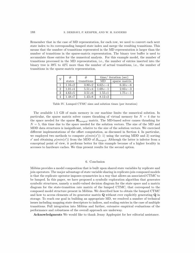
Remember that in the case of MD representation, for each row, we need to convert each nextstate index to its corresponding lumped state index and merge the resulting transitions. Thismeans that the number of transitions represented in the MD representation is larger than thenumber of transitions in the sparse-matrix representation. The binary tree buffer is used toaccumulate those entries for the numerical analysis. For this example model, the number oftransitions processed in the MD representation, i.e., the number of entries inserted into thebinary tree is 39% to 42% more than the number of actual transitions, i.e., the number oftransitions in the sparse-matrix representation.

N# # time/ iteration (sec)

states transitions MD sparse matrix1 1.16 e2 3.80 e2 6.62 e−4 6.33 e−62 1.01 e4 5.51 e4 1.69 e−1 2.83 e−33 4.63 e5 3.51 e6 1.55 e1 1.75 e−14 1.48 e7 1.43 e8 8.12 e2 –

Table IV. Lumped CTMC sizes and solution times (per iteration)

The available 1.5 GB of main memory in our machine limits the numerical solution. Inparticular, the sparse matrix solver causes thrashing of virtual memory for N = 4 due tothe space needed for the sparse Rlumped matrix. The MD-based solver causes thrashing forN = 5, this time due to the space needed for the solution vectors. The size of the MD andMDD data structures is insignificant, relative to the size of the solution vectors. We exerciseddifferent implementations of the offset computation, as discussed in Section 4. In particular,we employed two methods to compute ρ(min(s′)): 1) using the sorting MDD and 2) sortings′ and obtaining ρ(min(s′)) from the MDD of Slumped. Although the latter is inferior from aconceptual point of view, it performs better for this example because of a higher locality inaccesses to hardware caches. We thus present results for the second option.

6. Conclusion

Mobius provides a model composition that is built upon shared state variables by replicate andjoin operators. The major advantage of state variable sharing in replicate-join composed modelsis that the replicate operator imposes symmetries in a way that allows an associated CTMC tobe lumped. In this paper, we have proposed a symbolic exploration algorithm that generatessymbolic structures, namely a multi-valued decision diagram for the state space and a matrixdiagram for the state-transition rate matrix of the lumped CTMC, that correspond to thecomposed model structure present in Mobius. We described how to obtain the lumped CTMCand how to access elements of its generator matrix Q without ever explicitly generating Q instorage. To reach our goal in building an appropriate MD, we resolved a number of technicalissues including mapping state descriptors to indices, and scaling entries in the case of multipletransitions. Full integration into Mobius and further, extensive empirical evaluations of theperformance and robustness of the overall approach are underway.

Acknowledgments We would like to thank Jenny Applequist for her editorial assistance.


REFERENCES

1. R. E. Bryant. Graph-based algorithms for Boolean function manipulation. IEEE Trans. Comp., 35(8):677–691, Aug. 1986.

2. P. Buchholz. Markovian process algebra: Composition and equivalence. In Proc. 2nd Workshop on Proc.Algebras and Perf. Modelling, volume 27 of Arbeitsberichte des IMMD, pages 11–30, 1994.

3. P. Buchholz, G. Ciardo, S. Donatelli, and P. Kemper. Complexity of memory-efficient Kronecker operationswith applications to the solution of Markov models. INFORMS J. on Computing, 12(3):203, 2000.

4. J. R. Burch, E. M. Clarke, and K. L. McMillan. Symbolic model checking: 1020 states and beyond.Information and Computation, 98(2):142–170, June 1992.

5. G. Chiola, C. Dutheillet, G. Franceschinis, and S. Haddad. Stochastic well-formed colored nets andsymmetric modeling applications. IEEE Trans. on Computers, 42(11):1343–1360, November 1993.

6. G. Ciardo, G. Luttgen, and R. Siminiceanu. Saturation: An efficient iteration strategy for symbolic state-space generation. In TACAS 2001, volume 2031 of LNCS, pages 328–342. Springer, 2001.

7. G. Ciardo and A. Miner. Storage alternatives for large structured state spaces. In Proc. 9th Int. Conf.Modelling Techniques and Tools for Computer Performance Evaluation, volume 1245 of LNCS, pages44–57. Springer, 1997.

8. G. Ciardo and A. Miner. A data structure for the efficient Kronecker solution of GSPNs. In Proc. 8thInt. Workshop Petri Nets and Performance Models, pages 22–31, 1999.

9. G. Ciardo and A. Miner. Efficient reachability set generation and storage using decision diagrams. InProc. 20th Int. Conf. Application and Theory of Petri Nets, volume 1639 of LNCS, pages 6–25. Springer,1999.

10. E. M. Clarke, O. Grumberg, and D. Peled. Model Checking. MIT Press, 1999.11. D. D. Deavours, G. Clark, T. Courtney, D. Daly, S. Derisavi, J. M. Doyle, W. H. Sanders, and P. G.

Webster. The Mobius framework and its implementation. IEEE Trans. on Soft. Eng., 28(10):956–969,October 2002.

12. S. Derisavi, P. Kemper, W. H. Sanders, and T. Courtney. The Mobius state-level abstract functionalinterface. In Proc. of the 12th Int. Conf. on Modelling Techniques and Tools for Computer PerformanceEvaluation (TOOLS 2002), pages 31–50, 2002.

13. H. Hermanns, J. Kayser, and M. Siegle. Multi terminal binary decision diagrams to represent and analysecontinuous time Markov chains. In Proc. of 3rd Meeting on Numerical Solution of Markov Chains(NSMC),pages 188–207, 1999.

14. T. Ibaraki and N. Katoh. On-line computation of transitive closures of graphs. Information ProcessingLetters, 16:95–97, 1983.

15. K. Lampka and M. Siegle. Symbolic composition within the Mobius framework. InB. Wolfinger and K. Heidtmann, editors, Leistungs-, Zuverlassigkeits- und Verlasslichkeitsbewertung vonKommunikationsnetzen und verteilten Systemen, 2. MMB Arbeitsgesprach, pages 63–74. UniversitatHamburg, Fachbereich Informatik, Bericht 242, 2002.

16. D. Lee, J. Abraham, D. Rennels, and G. Gilley. A numerical technique for the evaluation of large, closedfault-tolerant systems. In Dependable Computing for Critical Applications 2 (DCCA-2), pages 95–114,1992.

17. A. Miner. Efficient solution of GSPNs using canonical matrix diagrams. In Proc. 9th Int. Workshop PetriNets and Performance Models, pages 101–110, 2001.

18. B. Plateau. On the stochastic structure of parallelism and synchronisation models for distributedalgorithms. In Proc. 1985 SIGMETRICS Conf. on Measurement and Modeling of Computer Systems,pages 147–153, 1985.

19. W. H. Sanders and L. M. Malhis. Dependability evaluation using composed SAN-based reward models.Journal of Parallel and Distributed Computing, 15(3):238–254, July 1992.

20. W. H. Sanders and J. F. Meyer. Reduced base model construction methods for stochastic activity networks.IEEE Journal on Selected Areas in Communications, 9(1):25–36, Jan. 1991.

21. A. Srinivasan, T. Kam, S. Malik, and R.E. Brayton. Algorithms for discrete function manipulation. InInt’l Conf. on CAD, pages 92–95, 1990.

22. W.J. Stewart. Introduction to the Numerical Solution of Markov Chains. Princeton, 1994.23. C. M. Woodside and Y. Li. Performance Petri net analysis of communications protocol software by delay-

equivalent aggregation. In Proc. of the 4th Int. Workshop on Petri Nets and Performance Models, pages64–73, 1991.

Date post:	23-Feb-2022
Category:	Documents
Upload:	others
View:	9 times
Download:	0 times

Symbolic State-space Exploration and Numerical Analysis of ...

Documents