Symmetric Relations and Geometric Characterizations about Standard Normal Distribution by Circle and Square
Shingo NAKANISHI And Masamitsu OHNISHI
Computing Center, Graduate School of Economics and
Center for Mathematical Modeling and Data Science, Osaka Institute of Technology, JAPAN Osaka University, JAPAN
Keywords: Standard Normal Distribution, Pythagorean theorem, Right Triangle, Tangent Line, Slope as Probability, Integral Form of Cumulative Distribution, Mills Ratio
1. Introduction Since ancient Babylonian, one of the human ancestors who had their civilizations by their own, found the way to measure or manage something for their communities to keep good conditions, their knowledge have been developed as one of the measuring methods with primitive mathematics and statistics [1, 2]. One was to use some digits or their squared numbers. After that, they draw the figures and pictures about the meaning of digits with some rules based on mathematics and geometry in ancient Egyptian civilization. Ancient Greeks also developed their cultural and artistic works. And they built many temples with beautiful architectural styles by using Pythagorean theorem [3] and some vivid proportions. For a long period including Medieval and Renaissance era, although they admitted various diversities and errors about something important under the uncertainties, the normal distribution had not been known yet because many famous works by researchers such as De Moivre in 1733, Laplace in 1812, Legendre in 1805, and Gauss in 1809 [4, 5] were unpublished. At that time of Renaissance era, it is said that da Vinci was interested in the relations about squares and circles [6] since these relations were very attractive and mysterious. And there was a question about squaring the circle [7] and were various religious cultures like Mandalas [8] during that time all over the world. By the way, since our human had our cultures to survive somehow, we have also understood that we experienced various opportunities for winning and losing about our economic environments. Bernstein explained to us about the markets as one of them. [2]. According to Ellis’s advice in his textbook [9], we should reduce our transaction cost not to lose the chances because over 1-year investigation brings us 60 percent of funds underperform, that over 10 years shows 70 percent underperform. And that over 20 years also shows 80 percent underperform for the chosen benchmarks. We think that there should be reduced a transaction cost and so on about almost of all things between winners and losers by a banker to get better utilities than they worry about unlucky results under the uncertainties. We also think that this is one modeling of the minus-sum games with thinking about the cost. This is what we proposed in our previous works like repetition games of coin tossing with their fees [10-14]. That is, we proposed that the sum-total of maximal profit for winners was equal to the cost by their banker based on about the probability 27 percent of standard normal distribution [10]. Based on the background we mentioned above, we have dealt with various kinds of characterizations [10-14] of a standard normal distribution at Pearson’s finding probability point 𝜆𝜆 = 0.612003 [15]. And its cumulative probability is 𝛷𝛷(−𝜆𝜆) =0.2702678 on a standard normal distribution. Kelley’s proposal, 𝜙𝜙(𝜆𝜆) = 2𝜆𝜆Φ(−𝜆𝜆) about 𝜆𝜆 = 0.612003, is called as 27 percent rule [16-21]. Especially, Sclove [21], Sclove and Johari [22] informed us of Cox’s proposal [23] about 𝜆𝜆 = 0.612003 as the important clustering of normal distribution. Nakamori et. al. [24] also mentioned that Cox’s study should be one of the original papers of K-means Algorisms. Our approaches [10-14] about 𝜆𝜆 = 0.612003 are also included as some of them. We found the other characterizations about 0.612003 from the parabola of the cost of the repetitions game of coin tossing [10] and the square on a standard normal distribution with several differential equations [11, 13, 14]. One of our proposals is about integral forms of a cumulative distribution of standard normal distribution [13, 14] in section 2. Another is related to both Mills ratio and inverse Mills ratio [13, 14] in section 3. In section 2, we would like to explain two types of the variable coefficient second order differential equations about standard normal distribution [13, 14, 25, 26] without mentioning 𝜆𝜆 = 0.612003 . We reconsider integral forms of cumulative distribution about standard normal distribution [13, 14] and Mills ratio about truncated normal distribution [25-31]. In section 3, we would like to clarify that Bernoulli differential equations of standard normal distribution [13, 14, 26] are geometrically related to 𝜆𝜆 = 0.612003 . Especially, we would like to show several characterizations based on their general solutions in section 2 and 3 are tied to a mathematical formulation [14]. In section 4, we would like to consider that the way such as ancient Egyptian drawing styles without imagining their depth. The height of inverse Mills ratios and integral forms of cumulative distribution of standard normal distribution are illustrated as various symmetric relations and geometric characterizations by using the drawing method. We clarify that the geometric
SETA2019 (The 15th International Symposium on Econometric Theory and Applications), Osaka University, Osaka, JAPAN, June 1st and 2nd, 2019
characterizations of general solutions both differential equations [13, 14, 26] about inverse Mills ratios [31-33] and that about integral forms of cumulative distribution on standard normal distributions inform us of crucial symmetric relations. At this time, we can show that 𝜆𝜆 = 0.612003 by Pearson [15], Kelley [16, 17], and Cox [23] should also play an important role in not only their symmetric relations but also the relation as the formulations for winners, losers and, a banker. Then, we can emphasize that the tangent lines on variable coefficient second order linear homogeneous differential equations [13, 14] are equal to these probabilities on a standard normal distribution by using Pythagorean theorem [3]. We would like to introduce the other attractive probability points we found instead of 𝜆𝜆(= 0.612003) throughout some illustrated figures concisely. From these examples, we can define that the probabilities of a standard normal distribution are two slopes of the tangent lines of the integral form of a cumulative distribution. We would like to show that it is an essential key for solving the relations about standard normal distribution by circle and square geometrically as one of the theoretical approaches for winners, losers and their banker in the field of econometrics. 2. Integral Forms of Cumulative Probability of Standard Normal Distribution and Reconfirmation about two types of
variable coefficient second order homogeneous differential equations If we think of a differential equation and its initial conditions as follows [13, 14]
ℎ𝑃𝑃′′(𝑢𝑢) + 𝑢𝑢ℎ𝑃𝑃′ (𝑢𝑢) − ℎ𝑃𝑃(𝑢𝑢) = 0, (2.1)
ℎ𝑃𝑃(0) = 𝜙𝜙(0) =1
√2𝜋𝜋, ℎ𝑃𝑃′ (0) =
12,
we can show you in the general solution with constants 𝐶𝐶𝑃𝑃1 and 𝐶𝐶𝑃𝑃2, where 𝜙𝜙(⋅) is a probability density function of standard normal distribution and 𝛷𝛷(⋅) is its cumulative distribution function.
From equation (2.2), the first derivative function is ℎ𝑃𝑃′ (𝑢𝑢) = 𝐶𝐶𝑃𝑃1𝛷𝛷(𝑢𝑢) + 𝐶𝐶𝑃𝑃2. (2.3)
Figure 1 Concepts of integral forms of cumulative distribution function of a standard normal distribution and visualizations about their variable coefficient second order differential equations symmetrically (Original Ref. [13]).
SETA2019 (The 15th International Symposium on Econometric Theory and Applications), Osaka University, Osaka, JAPAN, June 1st and 2nd, 2019
Therefore, since we understand that 𝐶𝐶𝑃𝑃1 = 1.0 and 𝐶𝐶𝑃𝑃2 = 0.0, we can estimate the solution [13, 14]
ℎ𝑃𝑃(𝑢𝑢) = 𝜙𝜙(𝑢𝑢) + 𝑢𝑢𝛷𝛷(𝑢𝑢). (2.4)
This equation is shown as 1-dot chain lines in the right of the bottom of Figure 1. Similarly, if we think of another initial condition as follows
ℎ𝑁𝑁′′(𝑢𝑢) + 𝑢𝑢ℎ𝑁𝑁′ (𝑢𝑢) − ℎ𝑁𝑁(𝑢𝑢) = 0, (2.5)
ℎ𝑁𝑁(0) = 𝜙𝜙(0) =1
√2𝜋𝜋, ℎ𝑁𝑁′ (0) = −
12,
we can also confirm the following equation [13, 14] ℎ𝑁𝑁(𝑢𝑢) = 𝜙𝜙(𝑢𝑢) − 𝑢𝑢𝛷𝛷(−𝑢𝑢). (2.6)
This is also shown symmetrically in the left of the bottom of Figure 1. Equations (2.4) and (2.6) are also described as
ℎ𝑃𝑃(𝑢𝑢) = � ℎ𝑃𝑃′ (𝜉𝜉)𝑑𝑑𝜉𝜉𝑢𝑢
−∞= � 𝛷𝛷(𝜉𝜉)𝑑𝑑𝜉𝜉
𝑢𝑢
−∞, (2.7)
ℎ𝑁𝑁(𝑢𝑢) = −� ℎ𝑁𝑁′ (𝜉𝜉)𝑑𝑑𝜉𝜉−𝑢𝑢
−∞= −� 𝛷𝛷(−𝜉𝜉)𝑑𝑑𝜉𝜉
−𝑢𝑢
−∞. (2.8)
By the way, although we can get the solutions ℎ𝑃𝑃(𝑢𝑢) = 𝜙𝜙(𝑢𝑢) + 𝑢𝑢𝛷𝛷(𝑢𝑢) and ℎ𝑁𝑁(𝑢𝑢) = 𝜙𝜙(𝑢𝑢) − 𝑢𝑢𝛷𝛷(𝑢𝑢) mentioned above, we would like to consider another type of differential equation [25, 26] as follows.
𝑚𝑚𝑃𝑃′′(𝑢𝑢) − 𝑢𝑢𝑚𝑚𝑃𝑃
′ (𝑢𝑢) −𝑚𝑚𝑃𝑃(𝑢𝑢) = 0,
𝑚𝑚𝑃𝑃(0) =√2𝜋𝜋
2 , 𝑚𝑚𝑃𝑃′ (0) = 1.0. (2.9)
From Equation (2.9), we can show you the general solution with constants 𝐶𝐶𝑃𝑃1 and 𝐶𝐶𝑃𝑃2 as follows
𝑚𝑚𝑃𝑃(𝑢𝑢) =𝐶𝐶𝑃𝑃1𝛷𝛷(𝑢𝑢) + 𝐶𝐶𝑃𝑃2
𝜙𝜙(𝑢𝑢) . (2.10)
Then, the first derivative function is shown as
𝑚𝑚𝑃𝑃′ (𝑢𝑢) =
𝐶𝐶𝑃𝑃1�𝜙𝜙(𝑢𝑢) + 𝑢𝑢𝛷𝛷(𝑢𝑢)� + 𝐶𝐶𝑃𝑃2𝑢𝑢𝜙𝜙(𝑢𝑢) . (2.11)
Since we can get the values 𝐶𝐶𝑃𝑃1 = 1.0 and 𝐶𝐶𝑃𝑃2 = 0.0, we can display the following solution as Mills ratio [14, 25, 26].
𝑚𝑚𝑃𝑃(𝑢𝑢) =𝛷𝛷(𝑢𝑢)𝜙𝜙(𝑢𝑢) . (2.12)
In the same way, if we have another condition [14] 𝑚𝑚𝑁𝑁′′(𝑢𝑢) − 𝑢𝑢𝑚𝑚𝑁𝑁
′ (𝑢𝑢) −𝑚𝑚𝑁𝑁(𝑢𝑢) = 0,
𝑚𝑚𝑁𝑁(0) =√2𝜋𝜋
2 , 𝑚𝑚𝑁𝑁′ (0) = −1.0, (2.13)
we can also display the following solution [14]
𝑚𝑚𝑁𝑁(𝑢𝑢) =1 −𝛷𝛷(𝑢𝑢)𝜙𝜙(𝑢𝑢) =
𝛷𝛷(−𝑢𝑢)𝜙𝜙(𝑢𝑢) . (2.14)
About two types of the differential equations, we would like to reconsider the relations mathematically as follows [14]. First, an inverse of 𝜙𝜙(𝑢𝑢) multiplied by Equation (2.4) is written as
ℒℎ𝑃𝑃(𝑢𝑢) =1
𝜙𝜙(𝑢𝑢)�𝑑𝑑2ℎ𝑃𝑃(𝑢𝑢)𝑑𝑑𝑢𝑢2 + 𝑢𝑢
𝑑𝑑ℎ𝑃𝑃(𝑢𝑢)𝑑𝑑𝑢𝑢 − ℎ𝑃𝑃(𝑢𝑢)� = 0. (2.15)
It is transformed into
ℒℎ𝑃𝑃(𝑢𝑢) = �ℎ𝑃𝑃′ (𝑢𝑢)𝜙𝜙(𝑢𝑢) �
′
− �ℎ𝑃𝑃(𝑢𝑢)𝜙𝜙(𝑢𝑢) � = 0. (2.16)
On the other hand, we can also rewrite Equation (2.15) as
SETA2019 (The 15th International Symposium on Econometric Theory and Applications), Osaka University, Osaka, JAPAN, June 1st and 2nd, 2019
Therefore, we can confirm Equations (2.16) and (2.19) are self-adjoint differential equations about standard normal distribution symmetrically. From Equations (2.12) and (2.14), a probability density of standard normal distribution is shown as
𝜙𝜙(𝑢𝑢) =1
𝑚𝑚𝑃𝑃(𝑢𝑢) + 𝑚𝑚𝑁𝑁(𝑢𝑢) . (2.21)
From Equations (2.4) and (2.12), we would like to confirm the following relation.
ℎ𝑃𝑃(𝑢𝑢)𝜙𝜙(𝑢𝑢) =
𝜙𝜙(𝑢𝑢) + 𝑢𝑢𝛷𝛷(𝑢𝑢)𝜙𝜙(𝑢𝑢) = 1 + 𝑢𝑢
𝛷𝛷(𝑢𝑢)𝜙𝜙(𝑢𝑢) = 𝑚𝑚𝑃𝑃
′ (𝑢𝑢). (2.22)
ℎ𝑃𝑃′ (𝑢𝑢)𝜙𝜙(𝑢𝑢) =
𝛷𝛷(𝑢𝑢)𝜙𝜙(𝑢𝑢) = 𝑚𝑚𝑃𝑃(𝑢𝑢) (2.23)
Then, we can insert equations (2.22) and (2.23) into (2.16) as follows.
�𝑚𝑚𝑃𝑃(𝑢𝑢)�′ − 𝑚𝑚𝑃𝑃′ (𝑢𝑢) = 0. (2.24)
Thus, Equation (2.24) is correct. Moreover, we can find the relations ℎ𝑃𝑃(𝑢𝑢) = 𝜙𝜙(𝑢𝑢)𝑚𝑚𝑃𝑃
′ (𝑢𝑢) (2.25)
and ℎ𝑃𝑃′ (𝑢𝑢) = 𝜙𝜙(𝑢𝑢)𝑚𝑚𝑃𝑃(𝑢𝑢). (2.26)
In the same way, Equation (2.6) and (2.14), we can clarify the following relation.
ℎ𝑁𝑁(𝑢𝑢)𝜙𝜙(𝑢𝑢) = −
𝜙𝜙(𝑢𝑢) − 𝑢𝑢𝛷𝛷(−𝑢𝑢)𝜙𝜙(𝑢𝑢) = −1 + 𝑢𝑢
𝛷𝛷(−𝑢𝑢)𝜙𝜙(𝑢𝑢) = −𝑚𝑚𝑁𝑁
′ (𝑢𝑢). (2.27)
ℎ𝑁𝑁′ (𝑢𝑢)𝜙𝜙(𝑢𝑢) =
𝛷𝛷(−𝑢𝑢)𝜙𝜙(𝑢𝑢) = −𝑚𝑚𝑁𝑁(𝑢𝑢) (2.28)
From equations (2.27) and (2.28), we can transform
�ℎ𝑁𝑁′ (𝑢𝑢)𝜙𝜙(𝑢𝑢) �
′
− �ℎ𝑁𝑁(𝑢𝑢)𝜙𝜙(𝑢𝑢) � = 0. (2.29)
into
�−𝑚𝑚𝑁𝑁(𝑢𝑢)�′ − �−𝑚𝑚𝑁𝑁′ (𝑢𝑢)� = 0. (2.30)
Thus, Equation (2.30) is also correct. Moreover, we can find the relation ℎ𝑃𝑃′ (𝑢𝑢) − ℎ𝑁𝑁′ (𝑢𝑢) = 1 (2.31)
and ℎ𝑁𝑁′ (𝑢𝑢) = −𝜙𝜙(𝑢𝑢)𝑚𝑚𝑁𝑁(𝑢𝑢) and ℎ𝑁𝑁(𝑢𝑢) = −𝜙𝜙(𝑢𝑢)𝑚𝑚𝑁𝑁
′ (𝑢𝑢) . (2.32)
SETA2019 (The 15th International Symposium on Econometric Theory and Applications), Osaka University, Osaka, JAPAN, June 1st and 2nd, 2019
3. Bernoulli Differential Equations for Inverse Mills Ratio In section 2, we considered that two types of the second order differential equations about a standard normal distribution. one is described in Figure 1 as the integral forms of a cumulative distribution function [13, 14]. The other is that about Mills Ratio [13, 14]. In this section, we would like to focus on the later type of differential equations and these relations based on 𝜆𝜆 = 0.612003. From Maddala’s explanation [27] and that of Johnson and Kotz [28], we can know that there are important censored and truncated normal distribution theories in these fields such as Tobit [29] and Heckman’s models [30]. We have already proposed the following formulations as Bernoulli differential equation with a standard normal distribution [13, 14].
If we reconsider the tendencies of an inverse Mills ratio and a hazard function [29] as the special cases on 𝜆𝜆 = 0.612003, we can illustrate the tendencies in Figure 2. From Figure 2, we can clarify that there are several relations between Equation (3.3) and (3.4) about the squares [11, 12] at 𝜆𝜆 on standard normal distribution if 𝐶𝐶 = 0. On the other hand, we can also display that maximal value 𝜙𝜙(𝜆𝜆)/𝛷𝛷(−𝜆𝜆) = 2𝜆𝜆 (in case of 𝑢𝑢 = ±𝜆𝜆) and ∓𝜆𝜆 which is the symmetric point on ±𝜆𝜆 about 0 is gotten as 2𝜆𝜆𝛷𝛷(−𝜆𝜆)�= 𝜙𝜙(𝜆𝜆)� shown in Figure 2 if 𝐶𝐶 = 𝛷𝛷(−𝜆𝜆) in Equation (3.3) and (3.4). Therefore, we can understand that the formulation [11, 16, 17] should be
𝜙𝜙(𝜆𝜆) = 2𝜆𝜆𝛷𝛷(−𝜆𝜆). (3.5)
Figure 2 Bernoulli differential equations of the ratios of probability density function of standard normal distribution out of its cumulative distribution function with thinking of its truncated normal distribution at the probabilistic point 𝜆𝜆 = 0.612003 and 𝜂𝜂 = 0.30263084 (Original Ref. [13]).
SETA2019 (The 15th International Symposium on Econometric Theory and Applications), Osaka University, Osaka, JAPAN, June 1st and 2nd, 2019
This Equation (3.5) plays a vital important role about the truncated normal distribution about ±𝜆𝜆 symmetrically and geometrically. By the way, the probability point, 𝜂𝜂 = 0.30263084 , is also a crucial important probability point because the value of cumulative distribution function is equal to that of probability density function at 𝜂𝜂 in Figure 2. We can find that it is another important relation since the inverse Mills ratio is equal to 1.0 in this case. Under the condition at 𝑢𝑢 = 0, we find the inverse Mills ratio is 2𝜙𝜙(0)(= 2/√2π) as 2 times of 𝜙𝜙(0). These geometric tendencies about Equations (3.3) and (3.4) separated by 𝑢𝑢 = 0 are also illustrated symmetrically in Figure 2. In section 4, we would like to explain that it is what we should emphasize about our proposals by using Pythagorean theorem in more detail. However, the equation such as Bernoulli differential equation with standard normal distribution is also mentioned by Hald [31]. Since we have been interested in the geometric characterizations of them and their relations with other differential equations in this section, we think of them as follows. First, the first order derivatives are shown as
𝑑𝑑𝑁𝑁′ (𝑢𝑢) =−𝑢𝑢𝜙𝜙(𝑢𝑢)(𝛷𝛷(−𝑢𝑢) + 𝐶𝐶) + 𝜙𝜙(𝑢𝑢)2
(𝛷𝛷(−𝑢𝑢) + 𝐶𝐶)2 , (3.6)
𝑑𝑑𝑃𝑃′ (𝑢𝑢) =−𝑢𝑢𝜙𝜙(𝑢𝑢)(𝛷𝛷(𝑢𝑢) + 𝐶𝐶) − 𝜙𝜙(𝑢𝑢)2
(𝛷𝛷(𝑢𝑢) + 𝐶𝐶)2 . (3.7)
If 𝐶𝐶 = 0, the first order derivatives are
𝑑𝑑𝑁𝑁′ (𝑢𝑢) =−𝑢𝑢𝜙𝜙(𝑢𝑢)𝛷𝛷(−𝑢𝑢) + 𝜙𝜙(𝑢𝑢)2
𝛷𝛷(−𝑢𝑢)2 =𝜙𝜙(𝑢𝑢)𝛷𝛷(−𝑢𝑢)
�𝜙𝜙(𝑢𝑢) − 𝑢𝑢𝛷𝛷(−𝑢𝑢)�𝛷𝛷(−𝑢𝑢) = −
𝑑𝑑𝑁𝑁(𝑢𝑢)ℎ𝑁𝑁(𝑢𝑢)ℎ𝑁𝑁′ (𝑢𝑢) = −
ℎ𝑁𝑁(𝑢𝑢)𝑚𝑚𝑁𝑁(𝑢𝑢)ℎ𝑁𝑁′ (𝑢𝑢) , (3.8)
𝑑𝑑𝑃𝑃′ (𝑢𝑢) =−𝑢𝑢𝜙𝜙(𝑢𝑢)𝛷𝛷(𝑢𝑢) − 𝜙𝜙(𝑢𝑢)2
𝛷𝛷(𝑢𝑢)2 = −𝜙𝜙(𝑢𝑢)𝛷𝛷(𝑢𝑢)
�𝜙𝜙(𝑢𝑢) + 𝑢𝑢𝛷𝛷(𝑢𝑢)�𝛷𝛷(𝑢𝑢) = −
𝑑𝑑𝑃𝑃(𝑢𝑢)ℎ𝑃𝑃(𝑢𝑢)ℎ𝑃𝑃′ (𝑢𝑢) = −
ℎ𝑃𝑃(𝑢𝑢)𝑚𝑚𝑃𝑃(𝑢𝑢)ℎ𝑃𝑃′ (𝑢𝑢) . (3.9)
Therefore, we can understand the general solutions of three types of differential equations are tied as an equation mathematically. Finally, we can define the relations about ℎ𝑃𝑃(𝑢𝑢),𝑚𝑚𝑃𝑃(𝑢𝑢), 𝑎𝑎𝑎𝑎𝑑𝑑 𝑑𝑑𝑃𝑃(𝑢𝑢) or ℎ𝑁𝑁(𝑢𝑢),𝑚𝑚𝑁𝑁(𝑢𝑢), 𝑎𝑎𝑎𝑎𝑑𝑑 𝑑𝑑𝑁𝑁(𝑢𝑢) as the following crucial important formulations
−𝑑𝑑𝑃𝑃′ (𝑢𝑢)𝑑𝑑𝑃𝑃(𝑢𝑢) =
ℎ𝑃𝑃(𝑢𝑢)ℎ𝑃𝑃′ (𝑢𝑢) =
𝑚𝑚𝑃𝑃′ (𝑢𝑢)
𝑚𝑚𝑃𝑃(𝑢𝑢) , (3.10)
−𝑑𝑑𝑁𝑁′ (𝑢𝑢)𝑑𝑑𝑁𝑁(𝑢𝑢) =
ℎ𝑁𝑁(𝑢𝑢)ℎ𝑁𝑁′ (𝑢𝑢) =
𝑚𝑚𝑁𝑁′ (𝑢𝑢)
𝑚𝑚𝑁𝑁(𝑢𝑢). (3.11)
4. Right Triangle for Probability of Standard Normal Distribution and its Truncated Normal Distribution In section 2, we mentioned some variable coefficient second order differential equations and their relations. In section 3, their differential equations and Bernoulli differential equations are connected by the fractions of Equation (3.10) about their primitive functions and first order derivatives. Since we have also found that the tangent lines of Equation (2.4) has important probabilistic characterizations shown in Figure 3 geometrically [13, 14], we would like to focus on our reconsiderations in section 2 as the integral forms of a cumulative distribution of a standard normal distribution. We have searched for their several characterizations such as Mills ratio [31-33], standard normal distribution [31, 34-35], their differential equations [36, 37], and the tendencies for winners, losers and a banker [2, 9, 10, 38]. From our investigations, we can propose that the general solutions of the variable coefficient second order differential equation in Figure 4 instead of our misspelled proposal [13, 14] inform us of several correct characterizations between statistics and geometry cooperatively as follows. From Figure 3, we can reconfirm the proportion for winners about per unit and per entire is equal to 𝜆𝜆 ∶ 𝜆𝜆𝛷𝛷(−𝜆𝜆) by our previous works [13, 14]. Its intercept form of a linear equation for winners [13] is shown as
−1𝜆𝜆 𝑢𝑢 +
1𝜆𝜆𝛷𝛷(−𝜆𝜆)𝑣𝑣 = 1. (4.1)
In the same way, we can define the intercept form of a linear equation for losers [13].
−1
𝜆𝜆 �1 + 𝛷𝛷(−𝜆𝜆)1 −𝛷𝛷(−𝜆𝜆)�
𝑢𝑢 +1
𝜆𝜆�1 + 𝛷𝛷(−𝜆𝜆)�𝑣𝑣 = 1. (4.2)
SETA2019 (The 15th International Symposium on Econometric Theory and Applications), Osaka University, Osaka, JAPAN, June 1st and 2nd, 2019
Figure 3 Geometric relationships between second order differential equations and standard normal distribution with a circle, squares, meaningful rectangles, their diagonals, and special tangent lines at 𝜆𝜆 = 0.612003 (Original Ref. [13]). Its proportion is equal to �1 + 𝛷𝛷(−𝜆𝜆)�/ �1− 𝛷𝛷(−𝜆𝜆)� ∶ �1 + 𝛷𝛷(−𝜆𝜆)�. From Equations (4.1) and (4.2), the intercept form for a banker [13] is also estimated as the following equation because of the proportion 1 ∶ 1. The meaning of per unit is that of per entire since the number of a banker should remain unit in this case. That is
−1𝜆𝜆 𝑢𝑢 +
1𝜆𝜆 𝑣𝑣 = 1. (4.3)
As described Equations (4.1) to (4.3), we can understand there are three intercept forms shown in Figure 3. At the same time, we can also confirm the crucial important tangent lines of ℎ𝑃𝑃(𝑢𝑢) at the probability points ±𝜆𝜆 as follows
Therefore, we can notice that 𝜙𝜙(𝜆𝜆) = 2𝜆𝜆𝛷𝛷(−𝜆𝜆) by Equation (3.5) is intercept of Equation (4.4) at 𝑢𝑢 = 0 shown in Figure 3. We can transform Equation (4.4) into the following intercept forms as our special proposals. Moreover, if we consider that both charts shown in Figures 2 and 3 as one picture such as Egyptian drawing styles without imaging their depth in Figure 4, we can also propose several modified intercept forms for Equations (4.1) to (4.3). That is, a modified intercept form of linear equation for a negative probability point −𝑥𝑥(= −𝜆𝜆) in Figure 4 is rewritten as
−1
𝜙𝜙(𝑥𝑥)𝛷𝛷(−𝑥𝑥)
𝑢𝑢 +1
𝜙𝜙(𝑥𝑥)𝑣𝑣1 = 1. (4.5)
Another modified intercept form of linear equation for a positive probability point 𝑥𝑥(= 𝜆𝜆) in Figure 4 is also rewritten as
−1
𝜙𝜙(𝑥𝑥)𝛷𝛷(𝑥𝑥)
𝑢𝑢 +1
𝜙𝜙(𝑥𝑥) 𝑣𝑣2 = 1. (4.6)
A modified intercept form of linear equation for probabilities both above negative probability point −𝑥𝑥(= −𝜆𝜆) and positive
SETA2019 (The 15th International Symposium on Econometric Theory and Applications), Osaka University, Osaka, JAPAN, June 1st and 2nd, 2019
probability point 𝑥𝑥(= 𝜆𝜆) in Figure 4 are shown as
−1
𝜙𝜙(𝑥𝑥)𝛷𝛷(𝑥𝑥) + 𝛷𝛷(−𝑥𝑥)
𝑢𝑢 +1
𝜙𝜙(𝑥𝑥) 𝑣𝑣 = 1 or −1
𝜙𝜙(𝑥𝑥)𝑢𝑢 +1
𝜙𝜙(𝑥𝑥) 𝑣𝑣 = 1. (4.7)
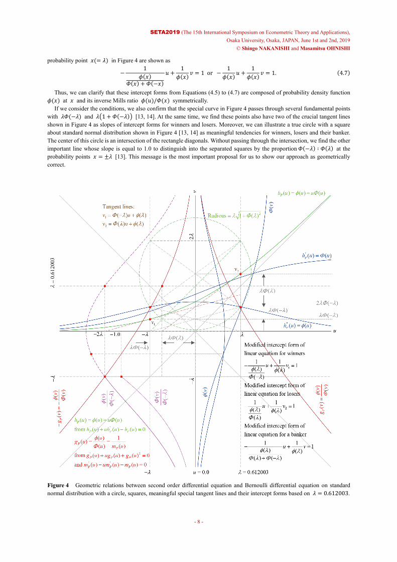
Thus, we can clarify that these intercept forms from Equations (4.5) to (4.7) are composed of probability density function 𝜙𝜙(𝑥𝑥) at 𝑥𝑥 and its inverse Mills ratio 𝜙𝜙(𝑢𝑢)/𝛷𝛷(𝑥𝑥) symmetrically. If we consider the conditions, we also confirm that the special curve in Figure 4 passes through several fundamental points with 𝜆𝜆𝛷𝛷(−𝜆𝜆) and 𝜆𝜆�1 + 𝛷𝛷(−𝜆𝜆)� [13, 14]. At the same time, we find these points also have two of the crucial tangent lines shown in Figure 4 as slopes of intercept forms for winners and losers. Moreover, we can illustrate a true circle with a square about standard normal distribution shown in Figure 4 [13, 14] as meaningful tendencies for winners, losers and their banker. The center of this circle is an intersection of the rectangle diagonals. Without passing through the intersection, we find the other important line whose slope is equal to 1.0 to distinguish into the separated squares by the proportion 𝛷𝛷(−𝜆𝜆) ∶ 𝛷𝛷(𝜆𝜆) at the probability points 𝑥𝑥 = ±𝜆𝜆 [13]. This message is the most important proposal for us to show our approach as geometrically correct.
Figure 4 Geometric relations between second order differential equation and Bernoulli differential equation on standard normal distribution with a circle, squares, meaningful special tangent lines and their intercept forms based on 𝜆𝜆 = 0.612003.
SETA2019 (The 15th International Symposium on Econometric Theory and Applications), Osaka University, Osaka, JAPAN, June 1st and 2nd, 2019
Furthermore, we would like to illustrate other probability points such as 𝑥𝑥 = 0.0 (𝛷𝛷(−0.0) = 0.5, 𝛷𝛷(0.0) = 0.5) and 𝑥𝑥 = ±0.67449 (𝛷𝛷(−0.67449) = 0.25, 𝛷𝛷(0.67449) = 0.75). These values 𝑥𝑥(= ±0.67449) are upper and lower quantiles [21]. They are also special points to explain our approach concretely shown in the top of Figure 5 since we can find that both the slopes of the right triangles at probability points ±𝑥𝑥 by using Pythagorean theorem are equal to these probabilities of standard normal distribution. If we estimate that 𝑥𝑥 = ±0.67449 , 𝑥𝑥 brings us the right triangle whose proportion is 3 ∶ 4 ∶ 5 by using Pythagorean theorem correctly and geometrically shown in Figure 5.
Figure 5 Various geometric characterizations between right triangles and probabilities on standard normal distribution by Pythagorean theorem. (Pythagorean theorem makes slopes and probabilities of standard normal distribution equally according to circle, square, and tangent lines.)
SETA2019 (The 15th International Symposium on Econometric Theory and Applications), Osaka University, Osaka, JAPAN, June 1st and 2nd, 2019
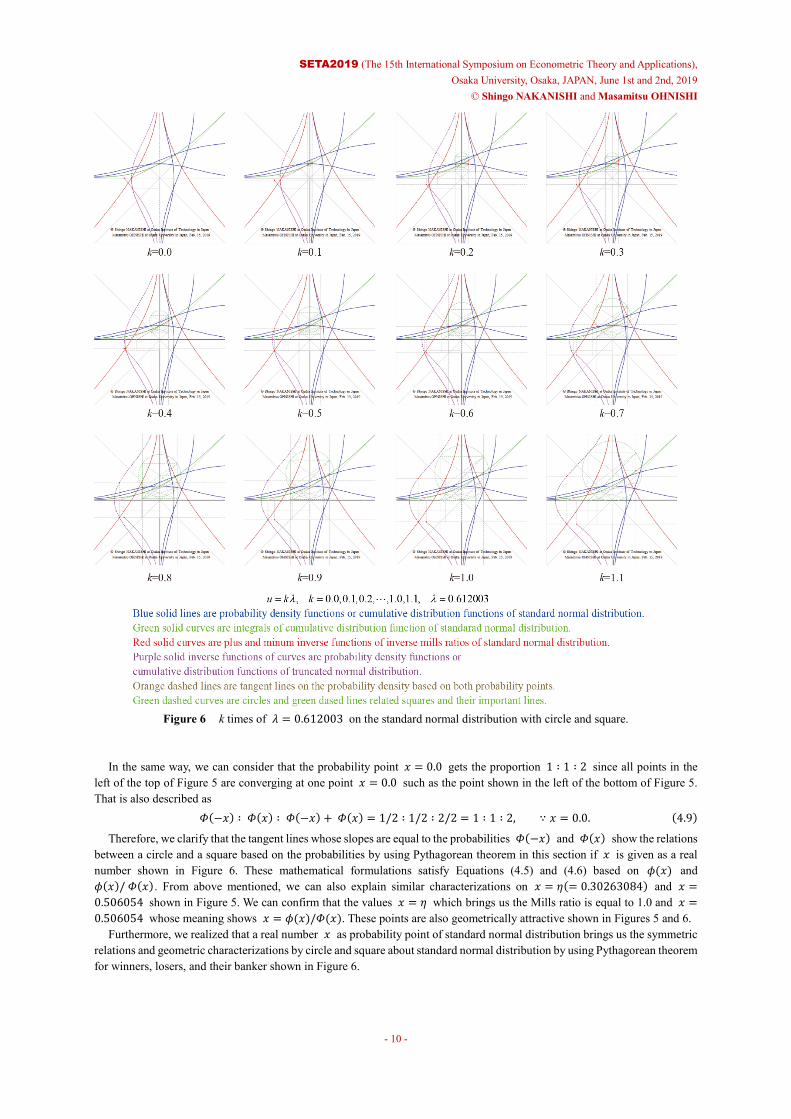
Figure 6 k times of 𝜆𝜆 = 0.612003 on the standard normal distribution with circle and square.
In the same way, we can consider that the probability point 𝑥𝑥 = 0.0 gets the proportion 1 ∶ 1 ∶ 2 since all points in the left of the top of Figure 5 are converging at one point 𝑥𝑥 = 0.0 such as the point shown in the left of the bottom of Figure 5. That is also described as
Therefore, we clarify that the tangent lines whose slopes are equal to the probabilities 𝛷𝛷(−𝑥𝑥) and 𝛷𝛷(𝑥𝑥) show the relations between a circle and a square based on the probabilities by using Pythagorean theorem in this section if 𝑥𝑥 is given as a real number shown in Figure 6. These mathematical formulations satisfy Equations (4.5) and (4.6) based on 𝜙𝜙(𝑥𝑥) and 𝜙𝜙(𝑥𝑥)/ 𝛷𝛷(𝑥𝑥) . From above mentioned, we can also explain similar characterizations on 𝑥𝑥 = 𝜂𝜂(= 0.30263084) and 𝑥𝑥 =0.506054 shown in Figure 5. We can confirm that the values 𝑥𝑥 = 𝜂𝜂 which brings us the Mills ratio is equal to 1.0 and 𝑥𝑥 =0.506054 whose meaning shows 𝑥𝑥 = 𝜙𝜙(𝑥𝑥)/𝛷𝛷(𝑥𝑥). These points are also geometrically attractive shown in Figures 5 and 6. Furthermore, we realized that a real number 𝑥𝑥 as probability point of standard normal distribution brings us the symmetric relations and geometric characterizations by circle and square about standard normal distribution by using Pythagorean theorem for winners, losers, and their banker shown in Figure 6.
SETA2019 (The 15th International Symposium on Econometric Theory and Applications), Osaka University, Osaka, JAPAN, June 1st and 2nd, 2019
5. Conclusions In this paper, we dealt with the symmetric relations and the geometric characterizations about a standard normal distribution by circle and square from the view point without imaging the height of densities such as Egyptian pictures in the ancient era. First, we can clarify that the general solutions as the integral form of cumulative distribution functions of standard normal distribution, Mills ratio, and inverse Mills ratio are shown as a mathematical formulation in section 3. In this case, we can confirm the integrals are related to inverse of Mills ratio. Second, from these tendencies, we can also get the modified intercept forms geometrically and symmetrically. We can understand these equations for winners, losers, and their banker according to the probability points. When the bottom line of the square is located on the height 𝑣𝑣 = 0.0, these probability points are 𝑢𝑢 =±𝜆𝜆 = ±0.612003 which are illustrated as the special case in our studies. Third, we can confirm that the integral form of a cumulative distribution function of standard normal distribution is expressed as Self-adjoint differential equation. As described above, we can reconfirm the geometric characterizations about 𝜆𝜆 = 0.612003 with considering square, circle, and normal distribution as the special modeling throughout this study. Furthermore, we can also realize there are many similar tendencies from European through Oriental historical cultures close to the relations between circles and squares such as Vitruvian man by Da Vinci [6], Squaring the Circle [7], and Mandalas [8]. There might not be related to normal distribution directly. However, the ancient Egyptian drawing styles enable us to illustrate symmetric relations and geometric characterizations between standard normal distribution and inverse Mills ratio with circle and square by using Pythagorean theorem as one of the greatest ancient Greek mathematical tools. We would like to expect that our proposals will be useful and contributed in the other fields as well as the statistical areas since our suggested charts and figures should be much simpler and more powerful than we thought. Acknowledgments
We would like to express our sincerely gratitude to Prof. Kosuke OYA and Prof. Hisashi TANIZAKI belonging to the Graduate School of Economics at Osaka University. The first author, Shingo NAKANISHI, would like to show my grateful to Prof. Hidemasa YOSHIMURA, Associate Prof. Manami SATO, Prof. Tsuneo ISHIKAWA and Prof. Yukimasa MIYAGISHI belonging to Osaka Institute of Technology. And the first author would particularly like to thank Prof. Takeshi KOIDE at Konan University, Associate Prof. Hitoshi HOHJO at Osaka Prefecture University, Prof. Shoji KASAHARA at Nara Institute of Science and Technology, Prof. Jun KINIWA at University of Hyogo. Especially, we would like to show full of our appreciations to Prof. Tetsuya TAKINE belonging to the Graduate school of Engineering at Osaka University, Prof. Hiroaki SANDOH at Kwansei Gakuin University and many other members at Operations Research Society of Japan (ORSJ) and Kansai-tiku Koryukai at the Securities Analysts Association of Japan (SAAJ). References [1] Stuart, I., “Why Beauty Is Truth: The History of Symmetry”, Basic Books, Kindle Edition, (2007). [2] Bernstein, P. L. “Against the Gods: The Remarkable Story of Risk”, Wiley, (1998). [3] Takloo-Bighash, R. “A Pythagorean Introduction to Number Theory: Right Triangles, Sums of Squares, and Arithmetic”, Springer,
(2018). [4] Hald, A., “A History of Probability and Statistics and their Applications before 1750”, John-Willey & Sons, (1990). [5] Wikipedia, “Normal distribution”, https://en.wikipedia.org/wiki/Normal_distribution, (Access month, July 2017). [6] Ida, T., “Vitruvian Man by Leonardo da Vinci and the Golden Ratio”, http://www.crl.nitech.ac.jp/~ida/education/VitruvianMan/index.html, (Access month: July 2017). [7] Wikipedia, “Squaring the Circle”, https://en.wikipedia.org/wiki/Squaring_the_circle, (Access month, November 2017). [8] Wikipedia, “Mandala”, https://en.wikipedia.org/wiki/Mandala, (Access month: July 2017). [9] Ellis, C. D., “Winning the Loser's Game, 6th edition: Timeless Strategies for Successful Investing”, McGraw-Hill Education, 6th edition,
(2013). [10] Nakanishi, S., “Maximization for sum total expected gains by winners of repetition game of coin toss considering the charge based on
its number trial”, Transactions of the Operations Research Society of Japan, 55, 1–26, (2012) in Japanese. [11] Nakanishi, S., “Uncertainties of active management in the stock portfolios in consideration of the fee”, Doctoral Thesis, Graduate School
of Economics, Osaka University, (17777), (2015) in Japanese. [12] Nakanishi, S., "Equilibrium point on standard normal distribution between expected growth return and its risk", Abstract of 28th
European Conference on Operational Research (the EURO XXVIII), Poznan, Poland, (2016). [13] Nakanishi, S. and Ohnishi, M., “Geometric Characterizations of Standard Normal Distribution - Two Types of Differential
Equations, Relationships with Square and Circle, and Their Similar Characterizations –”, Decision making theories under uncertainty and its applications: the extensions of mathematics for programming, RIMS Kôkyûroku, Research Institute for Mathematical Sciences, Kyoto University, No. 2078, pp. 58-64, (2018)
[14] Nakanishi, S. and Ohnishi, M. “Geometric Relations Between Standard Normal Distribution, Circle and Square by Risk and Returns”,
SETA2019 (The 15th International Symposium on Econometric Theory and Applications), Osaka University, Osaka, JAPAN, June 1st and 2nd, 2019
Modification version from misspelled edition about [13], The 15th workshop of the research group of OR of crisis and defense on November 22, 2018, National Graduate Institute for Policy Studies, Roppongi, Tokyo, JAPAN, Operations Research Society of Japan (ORSJ) (2018) in Japanese.
[15] Pearson, K., “On the probable errors of frequency constants”, Biometrika, 13, 113-32, (1920). [16] Kelley, T. L., “Footnote 11 to Jensen, MB, Objective differentiation between three groups in education (teachers, research workers, and
administrators)”, Genetic psychology monographs, 3(5), 361, (1928). [17] Kelley, T. L., “The selection of upper and lower groups for the validation of test items”, Journal of Educational Psychology, 30(1), 17-
24 (1939). [18] Mosteller, F., “On Some Useful Inefficient Statistics”, The Annals of Mathematical Statistics, 17, 377-408, (1946). [19] Cureton, E. E., “The upper and lower twenty-seven per cent rule”, Psychometrika, 22(3), 293-296, (1957). [20] Ross, J. and Weitzman, R. A., “The twenty-seven per cent rule”, The Annals of Mathematical Statistics, 214-221, (1964). [21] Sclove, S. L., “A Course on Statistics for Finance”, Chapman and Hall/CRC, (2012). [22] Johari, S. and Sclove, S. L., “Partitioning a distribution”, Communications in Statistics, A5, 133-147, (1976). [23] Cox, D. R., “Note on grouping”, Journal of the American Statistical Association, 52(280), 543-547, (1957). [24] Mar, S. O., Huynh, V.-N. and Nakamori, Y., “An alternative extension of the k-means algorithm for clustering categorical data”,
International Journal of Applied Mathematics and Computer Science, 14(2), 241-248, (2004). [25] Marsaglia, G., “Evaluating the Normal Distribution”, Journal of Statistical Software, Vol.11, Issue 4, pp.1-11, (2004). [26] Okagbue, H. I., Odetunmibi, O. A., Member, IAENG, Opanuga, A. A., Oguntunde, P. E., “Classes of Ordinary Differential Equations
Obtained for the Probability Functions of Half-Normal Distribution”, Proceedings of the World Congress on Engineering and Computer Science 2017, Vol. II, pp.876-882, (2017).
[27] Maddala, G. S. “Limited-Dependent and Qualitative Variables in Econometrics”, Cambridge University Press, (1983). [28] Jonson N. L. and Kotz, S., “Continuous Univariate Distributions-1”, John Willey & Sons, (1970). [29] Tobin, J., “Estimation of Relationships for Limited Dependent Variables”, Econometrica, 26, pp.24-36, (1958). [30] Heckman, J. J., “Shadow Prices, Market Wages, and Labor Supply”, Econometrica, 42(4), pp.679-694, (1974). [31] Hald, A., “Maximum Likelihood Estimation of the Parameters of a Normal Distribution which is Truncated at a Known Point”,
Scandinavian Actual Journal, 1949(1), pp.119-134, (1949). [32] Ahsanullah, M., Kibria, B.M.G. and Shakil, M., “Normal and Student´s t Distributions and Their Applications”, Atlantis Press, (2014). [33] Gordon, R. D., “Values of Mills' Ratio of Area to Bounding Ordinate and of the Normal Probability Integral for Large Values of the
Argument” The Annals of Mathematical Statistics, 12(3), 364-366, (1941). [34] Shibata, Y., “Normal Distribution – Characterizations and Applications –”, University of Tokyo, Press, (1981) in Japanese. [35] Bryc, W., “The Normal Distribution: Characterizations with Applications”, Springer New York, (1995). [36] Tenenbaum, M. and Pollard, H., “Ordinary Differential Equations”, Dover Publications, (1985). [37] Shinkai, H, “Ordinary Differential Equations with Structured Approach”, Kyoritsu Shuppan Co. Ltd. (2010) in Japanese. [38] Tanioka, I., “(Tsuki no Housoku in Japanese) Luck of Law, -Science about “How to Bet” and “Winning or losing””, PHP Lab., (1997)