68


Digitized by the Internet Archive
in 2011 with funding from
Boston Library Consortium IVIember Libraries
http://www.archive.org/details/symmetricallytriOOpowe
WS^^^mM9&SmiWM:
working paper
department
of economics
^SIMHETEICALLT TRIMMKI) LEAST SQUARES ESTIMATION
FOE TOBIT MODELS/
K. I.T. Workingby
: Paper #365
James L. Powell
August
,
1983 revised January, 1985
massachusetts
institute of
technology
50 memorial drive
Cambridge, mass. 02139

SIMHETEICALLT TRIMMED LEAST SQUARES ESTIMATION
FOE TOBIT MODELS/
M.I.T. Working Paper #365by
James L. PowellAugust, 1983 revised January, 1985
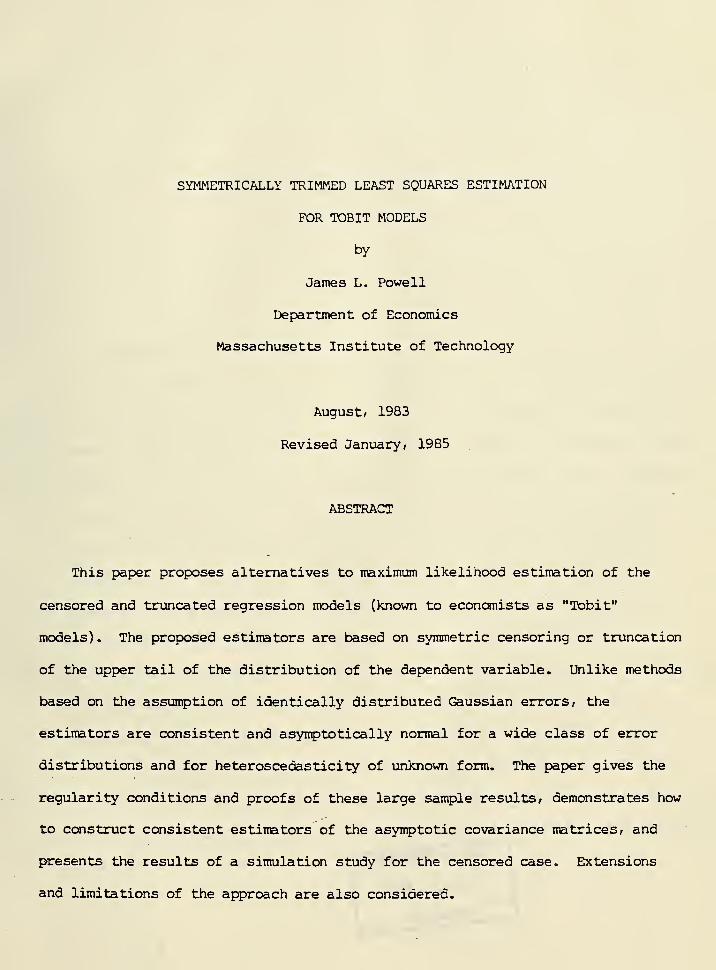
SYMMETRICALLY TRIMMED LEAST SQUARES ESTIMATION
FOR TOBIT MODELS
by
James L. Powell
Department of Economics
Massachusetts Institute of Technology
August/ 1983
Revised January/ 1985
ABSTRACT
This papjer proposes alternatives to maximum likelihood estimation of the
censored and truncated regression models (known to economists as "Tobit"
models) . The proposed estimators are based on symmetric censoring or truncation
of the upper tail of the distribution of the dependent variable. Unlike methods
based on the assumption of identically distributed Gaussian errors/ the
estimators are consistent and asymptotically normal for a wide class of error
distributions and for heteroscedasticity of unknown form. The paper gives the
regularity conditions and proofs of these large sample results, demonstrates how
to construct consistent estimators of the asymptotic covariance matrices, and
presents the results of a simulation study for the censored case. Extensions
and limitations of the approach are also considered.
SYMMETRICALLY TRIMMED LEAST SQUARES ESTIMATION
FOR TOBIT MODELsl/
by
James L. Powell
1 . Introduction
Linear regression models with nonnegativity of the dependent variable—known
to economists as "Tobit" models, due to Tobin's [1958] early investigation—are
commonly used in empirical economics, where the nonnegativity constraint is often
binding for prices and quantities studied. When the underlying error terms for
these models are known to be normally distributed (or, more generally, have
distribution functions with a known parametric form), maximum likelihood
estimation and other likelihood-based procedures yield estimators which are
consistent and asymptotically normally distributed (as shown by Amemiya [1973 J
"and Heckman [I979j)» However, such results are quite sensitive to the
"specification of the error distribution; as demonstrated by Goldberger [198OJ and
Arabmazar and Schmidt [1982 J, likelihood-based estimators are in general
inconsistent when the assumed parametric form of the likelihood function is
incorrect. Furthermore, heteroscedasticity of the error terms can also cause
inconsistency of the parameter estimates even when the shape of the error density
is correctly specified, as Hurd [1979J, Maddala and Kelson [1975J, and Arabmazar
and Schmidt [1981 J have shown.

Since economic reasoning generally yields no restrictions concerning the
form of the error distribution or homoscedasticity of the residuals, the
sensititivy of likelihood-based procedures to such assumptions is a serious
concern; thus, several strategies for consistent estimation without these
assumptions have been investigated. One class of estimation methods combines the
likelihood-based approaches with nonparametric estimation of the distribution
function of the residuals; among these are the proposals of Miller [1976 J,
Buckley and James [1979], Duncan [1983], and Fernandez [1985 J. At present, the
large-sample distributions of these estimators are not established, and the
methods appear sensitive to the assumption of identically distributed error
terms. Another approach was adopted in Powell [1984 J, which used a least
absolute deviations criterion to obtain a consistent and asymptotically normal
estimator of the regression coefficient vector. As with the methods cited above,
this approach applies only to the "censored" version of the Tobit model (defined
below), and, like some of the previous methods, involves estimation of the
density function of the error terms (which introduces some ambiguity concerning
2/the appropriate amount of "smoothing").—
In this study, estimators for the "censored" and "truncated" versions of the
Tobit model are proposed, and are shown to be consistent and asymptotically
normally distributed under suitable conditions. Ihe approach is not completely
general, since it is based upon the assumption of symmetrically (and
independently) distributed error terms; however, this assumption is often
reasonable if the data have been appropriately transformed, and is far more
general than the assumption of normality usually imposed. The estimators will
also be consistent if the residuals are not identically distributed; hence, they
are robust to (bounded) heteroscedasticity of unknovm form.
In the following section, the censored and truncated regression models are
defined, and the corresponding "symmetrically trimmed" estimators are proposed
and discussed. Section 3 gives sufficient conditions for strong consistency and
asymptotic normality of the estimators, and proposes consistent estimators of the
asymptotic covariance matrices for purposes of inference, while section 4
presents the results of a small scale simulation study of the censored
"symmetrically trimmed" estimator. The final section discusses some
generalizations and limitations of the approach adopted here. Proofs of the main
results are given in an appendix.
2. Definitions and Motivation
In order to make the distinction between a censored and a truncated
regression model, it is convenient to formulate both of these models as
appropriately restricted version of a "true" underlying regression equation
(2.1) y* = x'^p^ + u^, t = 1, ..., T,
where x. is a vector of predetermined regressors, p is a conformable vector of4/ O
unknown parameters, and u, is a scalar error term. In this context a censored
regression model will apply to a sample for which only the values of x, and
y = max{0, y*} are observed, i.e.,
(2.2) y^ = max{0, x^p^ + u^}
,
t = 1, ..., T.
The censored regression model can alternatively be viewed as a linear regression
model for which certain values of the dependent variable are "missing"—namely,
those values for which yf < 0. To these "incomplete" data points, the value zero
is assigned to the dependent variable. If the error term u. is continuously
distributed, then, the censored dependent variable y^ will be continuously
distributed for some fraction of the sample, and will assume the value zero for
the remaining observations.
A truncated regression model corresponds to a sample from (2.1) for which
the data point {y^, x^) is observed only when y1^ > 0; that is, no information
about data points with y1^ < is available. The truncated regression model thus
applies to a sample in which the observed dependent variable is generated from
(2.3) 7t = ^[^0 * ^V ^ ' ^' •••' "'
where Zj. and 6 are defined above and v. has the conditional distribution of u,t t t
given u+ > -zlP « That is, if the conditional density of Ux given x, is
f(Xlxa., t), the error term v^ will have density
(2.4) g(Xix^, t) = MX < -x'p^)f(X|x^, t)ir^. f(Xix^, t)dXr\V
where "1 (A)" denotes the indicator function of the event "A" (which takes the
value one if "A" is true and is zero otherwise).
If the trnderlying error terms {u+} were symmetrically distributed about
zero, and if the latent dependent variables {y+} were observable, classical least
squares estimation (under the usual regvdarity conditions) would yield consistent
estimates of the parameter vector p . Censoring or truncation of the dependent
variable, however, introduces an asymmetry in its distribution which is
systematically related to the repressors. The approach taken here is to
symmetrically censor or truncate the dependent variable in such a way that
symmetry of its distribution about xlp is restored, so that least squares will
again yield consistent estimators.
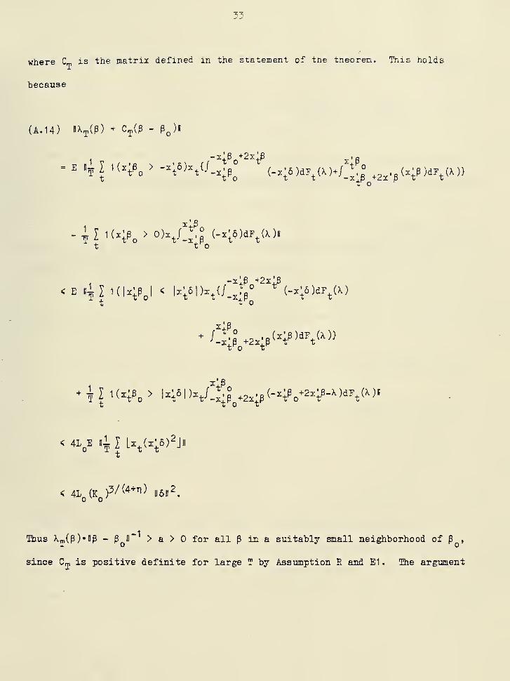
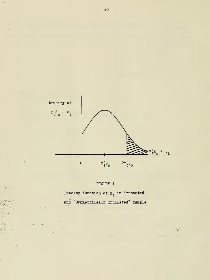
To make this approach more explicit, consider first the case in which the
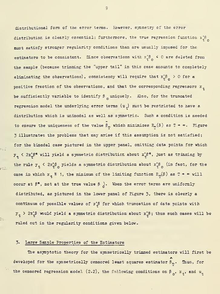
dependent variable is truncated at zero. In such a truncated sample, data points
for which u. < -^^Pq are omitted; but suppose data points with u. > ^t^n ^^'^^
also excluded from the sample. Then any observations for which xLp < would
automatically be deleted, and any remaining observations would have error terms
lying within the interval (-^tPn» ^tPn^' Because of the symmetry of the
distribution of the original error terms, the residuals for the "symmetrically
truncated" sample will also be sjonmetrically distributed about zero; the
corresponding dependent variable would take values between zero and
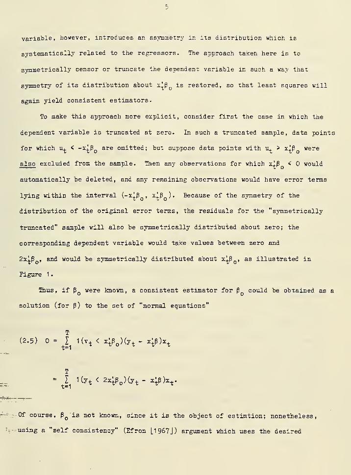
2xlp , and woiild be symmetrically distributed about xlp , as illustrated in
Pigure 1
.
Thus, if p were known, a consistent estimator for 6 coxild be obtained as a
solution (for P) to the set of "normal equations"
(2.5) = I l(v^< z;p^)(y^- z;p)x.
T
= I i(yt < 2x;p„)(yt- 4P)2^.X 1
Of course, P^ is not known, since it is the object of estimtion; nonetheless,
-using a "self consistency" (Efron [1967]) argument which uses the desired
estimator to perforn the "symmetric truncation," an estimator p„ for the
truncated regression model can be defined to satisfy the asymptotic "first-order
condition
T
(2.6) 0p(T^/^) = j^ l(y^ < 2x;p)(y^ - x;p)x^,
t=1
which sets the sample covariance of the regressors {x.} and the "symmetrically
trimmed" residuals {1 (-xlP < y+ - xlP < x'p)*(y. - 2:!p)} equal to zero
3/(asymptotically).— Corresponding to this implicit equation is a minimization
problem; letting (- -^)5R„(P)/dp denote the (discontinuous) right-hand side of
(2.6), the form of the function Rm(P) is easily found by integration:
T
(2.7) Ej(P) = I (y^ - ma2{^ y^, x^p}) .
t=1
Thus the symmetrically truncated least squares estimator p„ of P is defined as
any value of p which minimizes Em(P). over the parameter space B (assumed
compact).
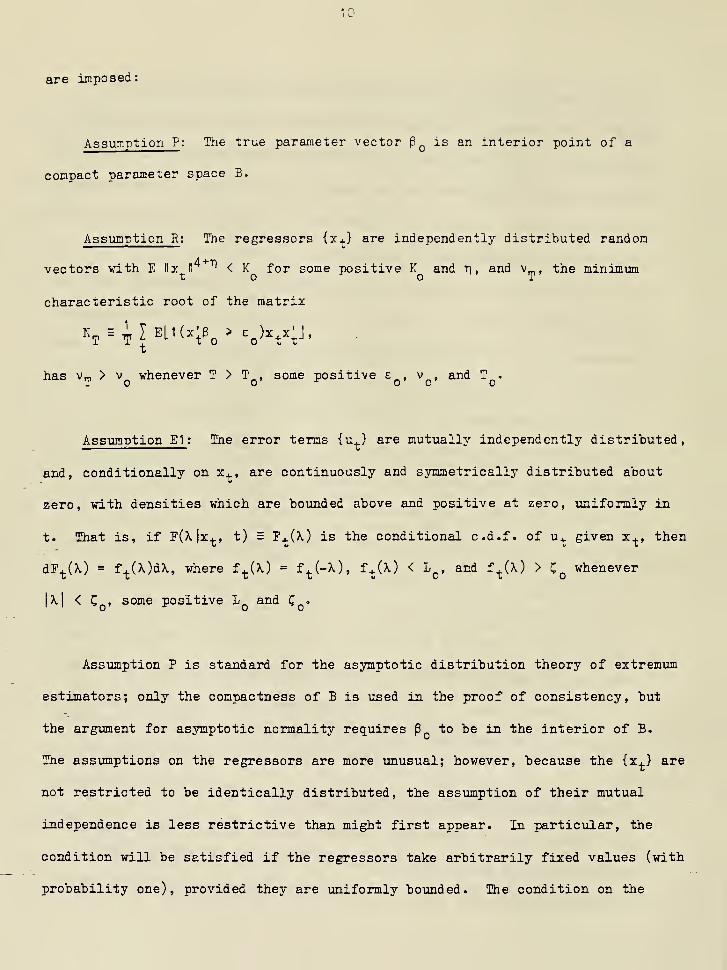
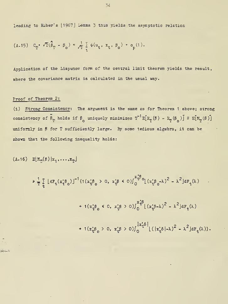
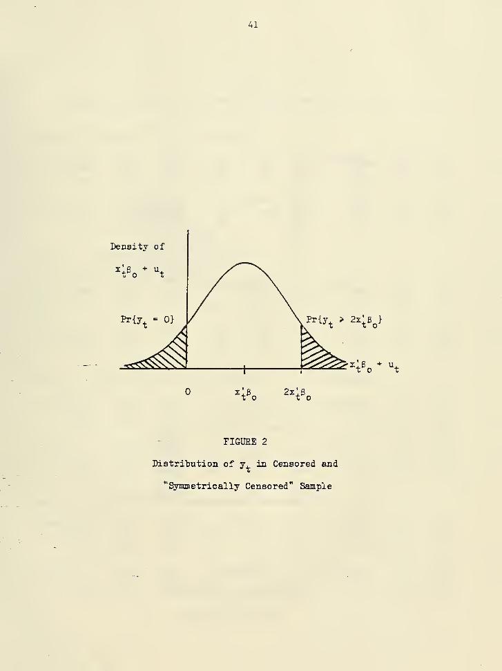
Definition of the symmetrically trimmed estimator for a censored sample is
similarly motivated. The error terms of the censored regression model are of the
form u? = max{u, , -x!p }, so "symmetric censoring" would replace u'^ with
min{u'^, 2;!p } whenever x!p > 0, and would delete the observation otherwise.
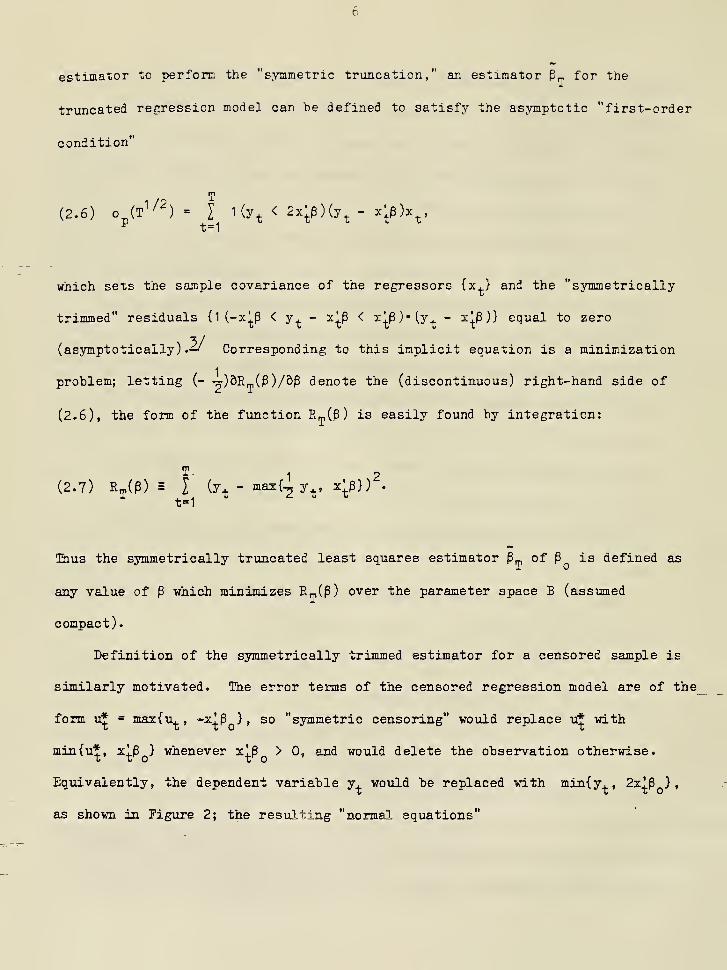
Equivalently, the dependent variable y, would be replaced with min{y, , 2z! p }
,
as shown in Figure 2; the resulting "normal equations"
T
(2.8) = I l(x'6 > 0)(min{y 2x'J } - x'p)^^' ,to tto ttt=1
for known P would be modified to
T
(2.9) = I l(x'^ > 0)(min{y^, 2x^p} " ^'^h^,t=1
since P is unknown. An objective function which yields this implicit equation
is
(2.10) Sj(P) = I (y^ - max{-^ y^, z;p} )'
+ I l(y^> 2x;p)[(-ly^)2- (max{0, z;p})2].
V 1
The symmetrically censored least squares estimator P of P is thus defined to be
any value of P minimizing S ip) over the parameter space B.
AThe reason P and P were defined to be minimizers of S (P) and IL(P),
rather than solutions to (2.6) and (2.9» respectively, is the multiplicity of
(inconsistent) solutions to these latter equations, even as T -> =>. The
"symmetric trimming" approach yields nonconvez minimization problems, (due to the
"^{x'3 > O)" term) so that multiple solutions to the "first-order conditions"
will ezist (for example, P = always satisfies (2.6) and (2.9))' Nevertheless,
under the regularity conditions to be imposed below, it will be shown that the
global minimizers of (2.7) and (2.10) above are unique and close to the true
value Po with high probability as !->•".
It is interesting to compare the "symmetric trimming" technique for the
censored regression model to the "EM algorithm" for computation of maximum
likelihood estimates when the parametric form of the error distribution is
assimed known.— This method computes the maximum likelihood estimate 6* of 6 asToan interative solution to the equation
(2.11) P*T= tl-rf-^I A(PV-tX X
where
y if y >
(2.12) 3-^ (P) ={
*
E(y* = x'P + uIu, < -x'p) otherwise.
^at is, the censored observations, here treated as missing values of y^, are
replaced by the conditional expectations of y* evaluated at the estimated value
P* (as well as other estimates of unknown nuisance parameters). It is the
calculation of the functional form of this conditional expectation that requires
knowledge of the shape of the error density. On the other hand, the
symmetrically censored least squares estimator p„ solves
(2.13) Pj = [I K^^Pj > 0)x^x;r''l l(x;p^ > 0)-min{y^, 2x;Pj}x^;X X
instead of replacing censored values of the dependent variable in the lower tail
of its distribution, the "symmetric trimming" method replaces uncensored
o"bservations in the upper tail by their estimated "symmetrically censored"
values.
The rationale behind the symmetric trimming approach makes it clear that
consistency of the estimators will require neither homoscedasticity nor known
distributional form of tne error terms. However, symmetry of the error
distribution is clearly essential; furthermore, the true regression function x'Pt
mus t satisfy stronger regularity conditions than are usually imposed for the
estimators to be consistent. Since observations with x'B < are deleted from
the sample (because trimming the "upper tail" in this case amounts to completely
eliminating the observations) , consistency will require that x!P > for aX o
positive fraction of the observations, and that the corresponding regressors x
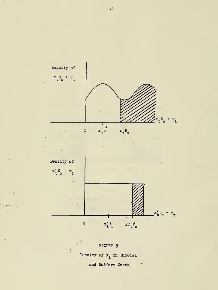
be sufficiently variable to identify p uniquely. Also, for the truncated
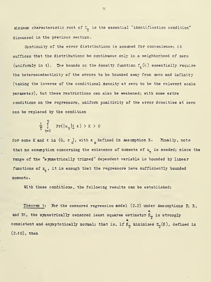
regression model the underlying error terms (u } must be restricted to have a
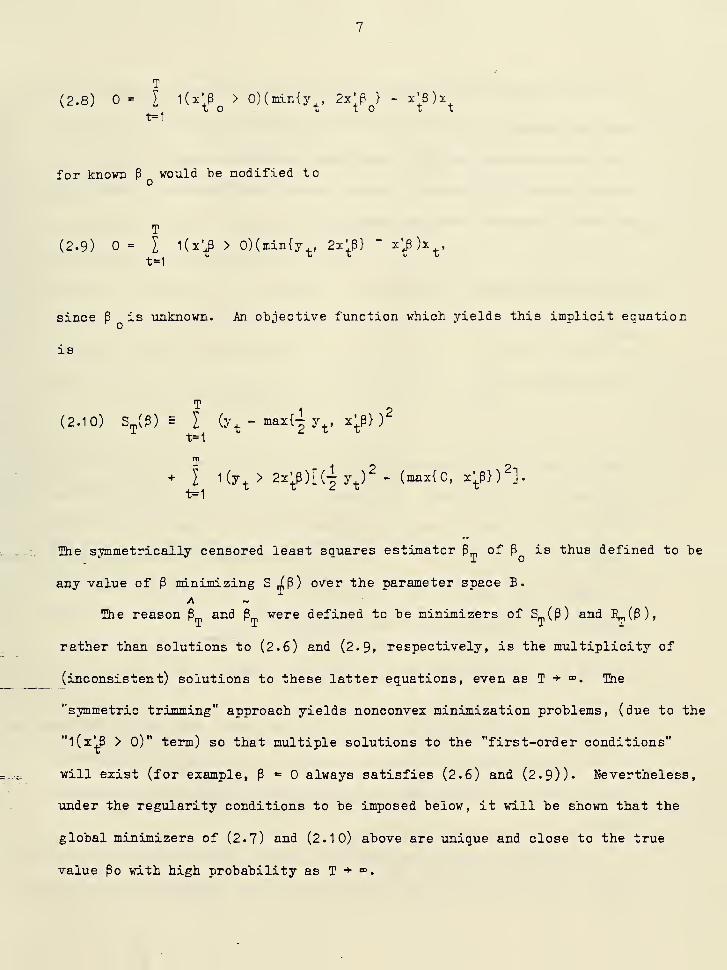
distribution which is unimodal as well as symmetric. Such a condition is needed
to ensure the uniqueness of the value p which minimizes En,(P) as T -* ". Figure
3 illustrates the problems that may arise if this assumption is not satisfied;
for the bimodal case pictured in the upper panel, omitting data points for which
y < 2z'P* will yield a symmetric distribution about x'B*, just as trimming byXX X
the rule y < 2x'P yields a symmetric distribution about x'B (in fact, for theI w X O Lf D
case in which z. = 1, the minimum of the limiting function E,p(P) as T -> => willX J,
occur at P*, not at the true value P ). ¥hen the error terms are uniformly
distributed, as pictured in the lower panel of Figure 3> there is clearly a
continuum of possible values of x'3 for which truncation of data points with
y. > 2z'P wDuld yield a symmetric distribution about x'3 ; thus such cases will be
ruled out in the regularity conditions given below.
3- Large Sample Properties of the Estimators
Ihe asymptotic theory for the symmetrically trimmed estimators will first be
developed for the symmetrically censored least squares estimator P„. Thus, for
the censored regression model (2.2), the following conditions on P , x,, and uOX X
on
10
are imposed:
Assum-ption P : The true parameter vector ^^ is an interior point of a
compact parameter space B.
Assumption E : The regressors {x;+-} are independently distributed rand
vectors with E llx, II ^ < K for some positive K and ti , and v_, the minimvmit o o T
characteristic root of the matrix
has Vm > V whenever T > T„, some positive e„, v , and T .To ^
Assimption E1 : The error terms {u^} are mutually independently distributed,
and, conditionally on x+, are continuously and symmetrically distributed about
zero, with densities which are bounded above and positive at zero, uniformly in
t. That is, if F(X |x^, t) = "P+M is the conditional c.d.f. of u^ given x^, then
dF^(X) = f^{X)iX, where f^(X) = f^*'"^^' ^t^^^ "^
-"^o'^^'^
^t^^^ ^ ^o"^s^®"^®^
|X| < Cq, some positive L and C^-
Assumption P is standard for the asymptotic distribution theory of extremum
estimators; only the compactness of B is used in the proof of consistency, but
the argument for asymptotic normality requires p to be in the interior of B.
The assimptions on the regressors are more unusual; however, because the {x+} are
not restricted to be identically distributed, the assumption of their mutual
independence is less restrictive than might first appear. In particiilar, the
condition will be satisfied if the regressors take arbitrarily fixed values (with
probability one), provided they are xmiformly bounded. The condition on the
11
ininimuin characteristic root of K is the essential "identification condition"
discussed in the previous section.
Continuity of the error distributions is assumed for convenience; it
suffices that the distributions be continuous only in a neighborhood of zero
(uniformly in t) . The bounds on the density function f.i'k) essentially require
the heteroscedasticity of the errors to be bounded away from zero and infinity
(taking the inverse of the conditional density at zero to be the relevant scale
parameter), but these restrictions can also be weakened; with some extra
conditions on the regressors, uniform positivity of the error densities at zero
can be replaced by the condition
1^
i 1 Pr(|u |< O > K >
^ t=1 ^
for some K and e in (O, e ), with e defined in Assumption E. finally, note
that no assumption concerning the ezistence of moments of u is needed; since the
range of the "symmetrically trimmed" dependent variable is bounded by linear
functions of s , it is enough that the regressors have sufficiently bounded
moments.
¥ith these conditions, the following results can be established:
Theorem 1 : Ibr the censored regression model (2.2) under Assumptions P, E,
Aand El , the symmetrically censored least squares estimator p„ is strongly
Aconsistent and asymptotically normal; that is, if P minimizes S_(P), defined in
(2.10), then
12
A(i) lim P„ = P almost surely, and
(ii) L-^/^C^-/T(P^ - h^ ^ "^°' ^^'
where
-1 /2and I'm is any square root of the inverse of
D, ^ I ELl(x;P^ > 0).nin{u2, (^VS^^'"''
The proof of this and the following theorems are given in the mathematical
appendix below.
Turning now to the truncated regression model (2.3)~(2.4), additional
restrictions must be imposed on the error distributions to show consistency and
asymptotic normality of the symmetrically trimmed estimator P^,:
Assumption E2 ; In addition to the conditions of Assumption E1 , the error
densities {f. (X)} are unimodal, with strict unimodality, uniformly in t, in some
neighborhood of zero. That is, f, (Xp) *• f+C^^) if |X.|
> IXpl, and there exists
some a > and some function h(X), strictly decreasing in [0, o J, such that
^^(^2^ - f^i>^^) > h{\X^\) - h(|X^l) when \\^\ < \X^\ < a^.

13
With these additional conditions, results similar to those in Theorem 1 can
be established for the truncated case.
Theorem 2: For the truncated regression model (2.5)~(2.4) under Assumptions
P, E, and E2, the symmetrically truncated least squares estimator P^ is strongly
consistent and asymptotically normal; that is, if p minimizes P^ (p ) , defined in
(2.7), then
(i) lim p = p almost surely, and
(ii) Z-^/2(^^ . Y^).»^(P^ - P^) ^ N(0, I), where
w^ = ^ I eLi(-x;p^ < v^ < ^;p,)x,x;j,
X
t t t
and Zl ' is any square root of the inverse of
Zj= ;iELi(-x;p^< v^< x;p^)v2x^x;].
In order to use the asymptotic normality of Pm and P_ to construct large
sample hypothesis tests for the parameter vector p , consistent estimators of the
asymptotic covariance matrices must be derived. For the censored regression
model, "natural" estimators of relevant matrices Cm and Dm exist; they are
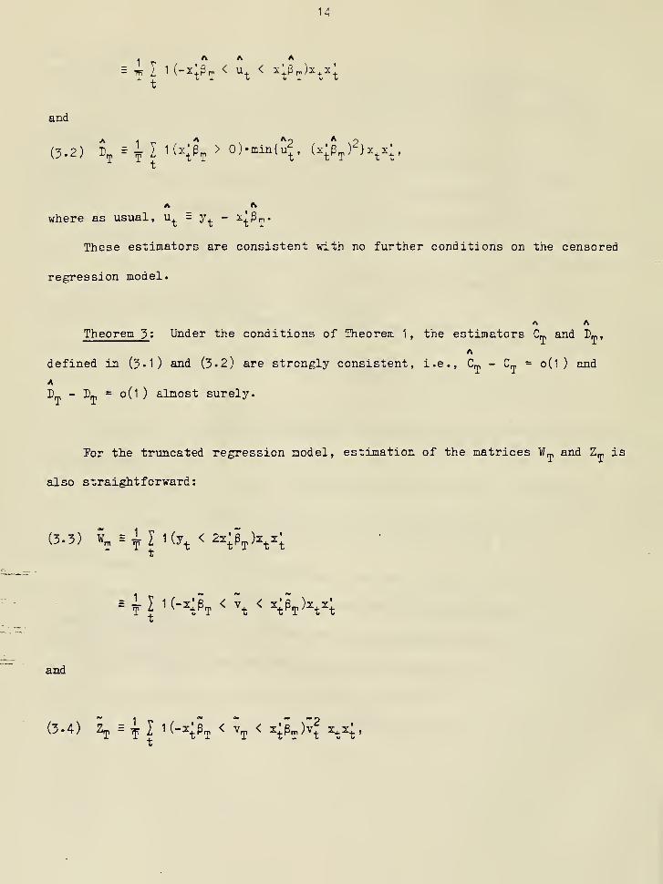
(3.1) Cj^I 1(0 <y, < 2x;p^)x^z;X
and
14
, AAA
A 1 r. , .**
, .'^2 *
(3.2) Dy ^I 1(^;Pt > O)*'^^^^^'(^i^T^^^^t^^
where as usual, u^ = y^ - x^Prp-
These estimators are consistent with no further conditions on the censored
regression model.
A ATheorem 3 : Under the conditions of Theorem 1 , the estimators Cm and D™,
A
defined in (3.1) and (3.2) are strongly consistent, i.e., C^ - Cm = o(l ) and
A
E - Dm = o(l ) almost surely.
For the truncated regression model, estimation of the matrices Wm and Z™ is
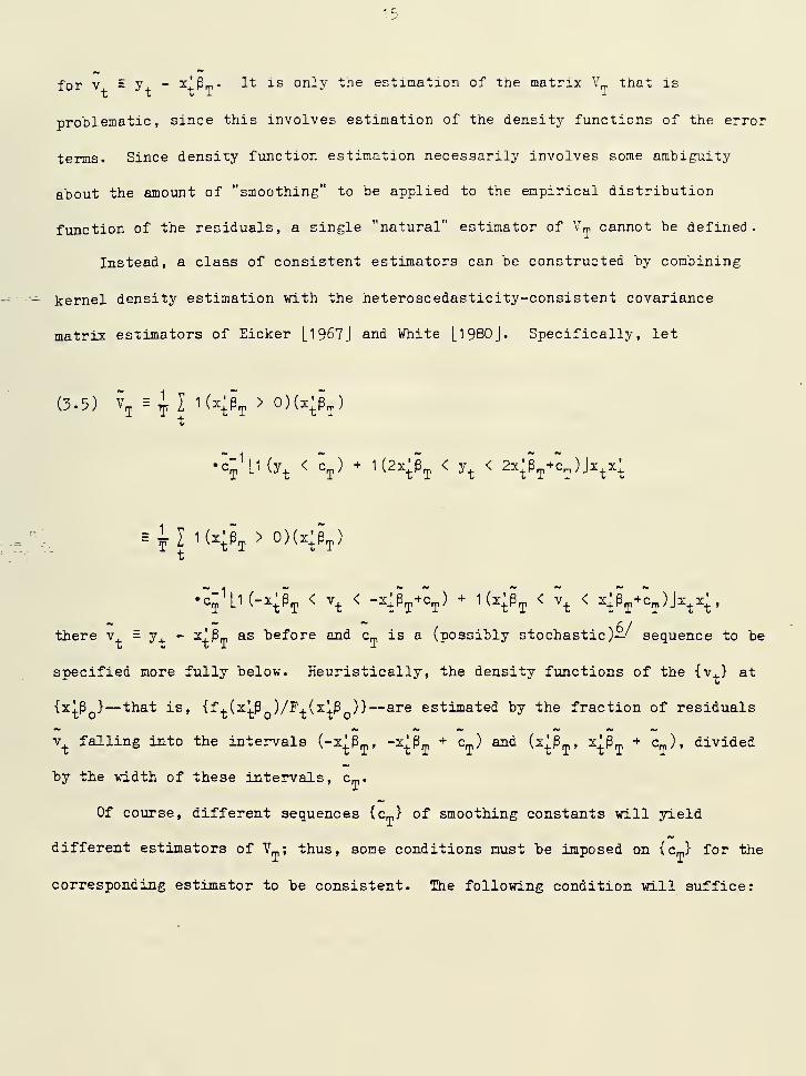
also straightforward:
(3.3) \=^Il(y, <2::;Pt)v;
_ 1lli(-;p, < v^<x;p^)v;
and
(3.4) Zj = ^ I 1 (-z;Pt ^"^T
^ ^t^T^^^t ""t^'X
15
for V - y+ - ^+Pm- I't is only the estimation of the matrix Y„ that is
problematic, since this involves estimation of the density functions of the error
terms. Since density function estimation necessarily involves some ambiguity
about the amount of "smoothing" to be applied to the empirical distribution
function of the residuals, a single "natural" estimator of Vrp cannot be defined.
Instead, a class of consistent estimators can be constructed by combining
-— kernel density estimation with the heteroscedasticity-consistent covariance
matrix estimators of Eicker [1967] and White [1980 J. Specifically, let
(3.5) v^ =-jv I i(x;pt > °^(^t^T^
:-i•c-'[l(y^ < c^) - l(2x;p^ < y^ < 2x;p^.c^)Jx^x;
_ 1
there v ,= y ,
- ^l^m as before and c„ is a (possibly stochastic)—'^ sequence to be
specified more fully below. Heuristically, the density functions of the {v.} at
{zip }— that is, {f+(2lp )/F,(xlP )}—are estimated by the fraction of residuals
\ falling into the intervals (-^^P^t "^t^T"^
'^T^^^
^^t^T' ^t^T"^
^T^''^^"^^'^®^
by the width of these intervals, Cn,.
Of course, different sequences (Cm) of smoothing constants will yield
different estimators of ¥_; thus, some conditions must be imposed on (cm) for the
corresponding estimator to be consistent. The following condition will suffice:
16
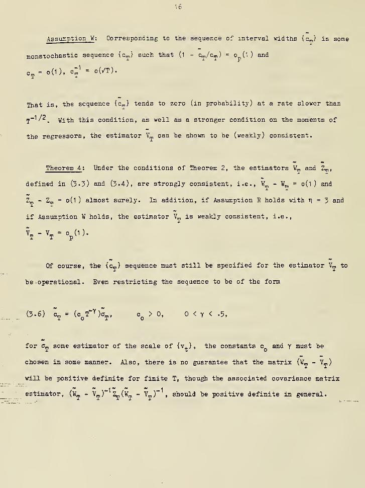
Assunption W : Corresponding to the sequence of interval widths {c,^} is some
monstochastic sequence {c,t,} such that (l - c^/crp) = o (l ) and
c^= 0(1), c-^ = o(/T).
That is, the sequence {c™} tends to zero (in probability) at a rate slower than
T~ ' . With this condition, as well as a stronger condition on the moments of
the regressors, the estimator V_, can be shown to be (weakly) consistent.
Theorem 4 : Under the conditions of Theorem 2, the estimators V.' and Zm,
defined in (3-3) and (3-4), are strongly consistent, i.e., W - W = o(l ) and
Zn, - Z_ = 0(1 ) almost surely. In addition, if Assumption R holds with ti = 3 and
if Assxmption ¥ holds, the estimator V_ is weakly consistent, i.e.,
V, -Vj = o^(l).
Of course, the {cm) sequence must still be specified for the estimator Vm to
"be -operational. Even restricting the sequence to be of the form
(3.6) c^ = (c^T"^)aj, =0 ^ °' < Y < .5,
for a^ some estimator of the scale of {v, } , the constants c and v must beT t
chosen in some manner. Also, there is no guarantee that the matrix (vr_ - Vm)
will be positive definite for finite T, though the associated covariance matrix
estimator, (W„ => V^)' Z|p(W_ - V_)~ , should be positive definite in general.

17
Thus, further research on the finite sample properties of V^ is needed before it
can be used with confidence in applications.
Given the conditions imposed in Theorems 1 through 4 above, normal sampling
theory can be used to construct hypothesis tests concerning P^ without prior
knowledge of the likelihood function of the data. In addition, the estimators p
and P can be used to test the null hypothesis of homoscedastic , normally-
distributed error terms by comparing these estimators with the corresponding
maximum likelihood estimators, as suggested by Hausman [1978 J. Of course,
rejection of this null hypothesis may occur for reasons which cause the
symmetrically- trimmed estimators to be inconsistent as well— e.g., asjnnmetry of
7/the error distribution, or misspecification of the regression function.—
4-. Finite Sample Behavior of the Symmetrically Censored Estimator
Having established the limiting behavior of the symmetrically trimmed
estimators under the regularity conditions imposed above, it is useful next
to consider the degree to which these large sample results apply to sample
sizes likely to be encountered in practice. To this end, a small-scale
simulation study of a bivariate regression model was conducted, using a
variety of assumptions concerning sample size, degree of censoring, and error
distribution. It is, of course, impossible to completely characterize the
Afinite-sample distribution of g^, under the weak conditions imposed above;
Anonetheless, the behavior of p^ iJi a few special cases may serve as a guide
to its finite sample behavior, and perhaps as well to the sampling behavior
of the symmetrically truncated estimator p^.
The "base case" simulations took the dependent variable y , to be
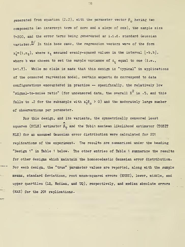
generated from equation (2.2), with the parameter vector P having two
components (an intercept term of zero and a slope of one), the sample size
T=200, and the error terms being genereated as i.i.d. standard Gaussian
variates.— In this base case, the regression vectors were of the form
xl.= {^,z±.), where z+ assumed evenly-spaced values in the interval L-b,bJ,
where b was chosen to set the sample variance of z, equal to one (i.e.,
b"='1.7). While no claim is made that this design is "typical" in applications
of the censored regression model, certain aspects do correspond to data
configurations encountered in practice — specifically, the relatively low
2"signal-to-noise ratio" (for uncensored data, the overall E is .5» and this
falls to .2 for the subsample with x|P_ > 0) and the moderately large number
of observations per parameter.
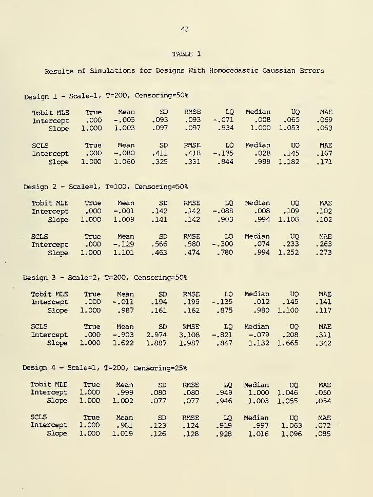
For this design, and its variants, the symmetrically censored least
squares (SCLS) estimator P_ and the Tobit maximum likelihood estimator (TOBIT
MLE) for an assumed Gaussian error distribution were calculated for 201
replications of the experiment. The results are summarized under the heading
"Design 1" in Table 1 below. The other entries of Table 1 summarize the results
for other designs which maintain the homoscedastic Gaussian error distribution.
For each design, the "true" parameter values are reported, along with the sample
means, standard deviations, root mean-squared errors (R14SE), lower, middle, and
upper quartiles (LQ, Median, and UQ), respectively, and median absolute errors
(MAE) for the 201 replications.
19
One feature of the tabulated results which is not surprising is the
relative efficiency of the Gaussian KLE (which is the "true" KLE for these
designs) to the SCLS estimator for all entries in the table. Comparison of
the SCLS estimator to the MLE using the RKSE criterion is considerably less
favorable to SCLS than the same comparison using the KAE criterion,
suggesting that the tail behavior of the SCLS estimator is an important
determinant of this efficiency. The magnitude of the relative efficiency is
about what would be expected if the data were uncensored and classical least
squares estimates for the entire sample were compared to least squares
estimates based only upon those observations with x^P > 0; that is, the
approximate three- to-one efficiency advantage of the MLE can largely be
attributed to the exclusion (on average) of half of the observations having
A more surprising result is the finite sample bias of the SCLS
estimator, with bias in the opposite direction (i.e., upward bias in slope,
downward bias in intercept) from the classical least squares bias for
censored data. While
this bias represents a small conponent in the EMSE of the estimator, it is
interesting in that it reflects an asymmetry in the sampling distribution of
P,j, (as evidenced by the tabulated quartiles) rather than a "recentering" of
this distribution away from the true parameter values. In fact, this
asymmetry is caused by the interaction of the x'p < "exclusion" rule with
the magnitude of the estimated ^^ components. Specifically, SCLS estimates
with high slope and low intercept components rely on fewer observations for
their numerical values than those with low slope and high intercept terms
20
(since the condition "j^jPm > 0" occurs more frequently in the latter case);
as a result, high slope estimates have greater dispersion than low slope
estimates, and the corresponding distribution is skewed upward. Though this
is a second-order effect in terms of MSE efficiency, it does mean that
conclusions concerning the "center" of the sampling distributions will depend
upon the particular notion of center (i.e., mean or median) used.
The remaining designs in Table 1 indicate the variation in the sampling
distribution of P_ when the sample size, signal-to-noise ratio, censoring
proportion, and number of regressors changes. In the second design, a 30%
reduction of the sample size results in an increase of about /2 in the
standard deviations, and of more than /2 in the mean biases, in accord with
the asymptotic theory (which specifies the standard deviations of the
—1 /P —1 /Pestimators to be 0(T~ ' ) and the bias to be o(T~ ' )). Doubling the scale
2of the errors (which reduces the population K of the uncensored regression
to .2, and the E for the observations with z'p > to =06) has much moreto
drastic effects on the bias and variability of the SCLS estimator, as
illustrated by design 3; on the other hand, reduction of the censoring
proportion to 25% (hy increasing the intercept of the regression to one in
design 4) substantially reduces the bias of the SCLS estimator and greatly
improves its efficiency relative to the MLE (of course, as the censoring
proportion tends to zero, this efficiency will tend to one, as both estimators
reduce to classical least squares estimators).
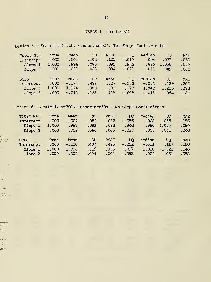
The last two entries of Table 1 illustrate the interaction of number of
parameters with sample size in the performance of the SCLS estimator. In
these designs, an additional regressor w , , taking on the repeating sequence
21
{-1 . 1 » 1 >"''»••• ^ of values; v. thus had zero mean, unit variance, and was
uncorrelated with z^ (both for the entire sample and the subsample vath
xlp > O), and its coefficient in the regression function was taken to be
zero, leaving the explanatory power of the regression unaffected. Comparison
of designs 5 and 6 with designs 1 and 2 suggest that the convergence of the
sampling distribution is slower than 0(p/n); that is, the sample size must
increase more than proportionately to the number of regressors to achieve the
same precision of the sampling distribution.
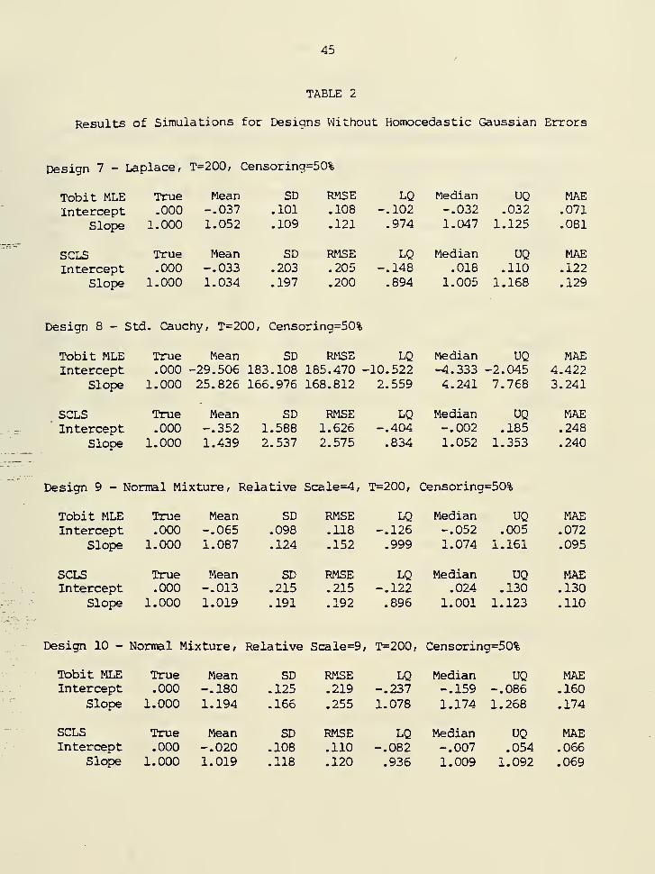
In Table 2, the design parameters of the base case — T=200, censoring
proportion = 50^, and overall error variance = 1 (except for design 8, which
used the standard Cauchy distribution) — are held fixed, and the effects of
departures of the error distribution from normality and homoscedasticity are
investigated. For these experiments, the RMSE or MAE efficiency of the SCLS
estimator to the Gaussian MLE depends upon whether the inconsistency of the
latter is numerically large relative to its dispersion. In the Laplace
example (design 6), the 3% bias in the MLE slope coefficient (which reflects
an actual recentering of the sampling distribution rather than asymmetry) is
a small component of its EMSE, which is less than that for the SCLS
estimator; with Cauchy errors, the performance of the Gaussian MLE
deteriorates drastically relative to symmetrically censored least squares.
For the ^0% normal mixtures of designs 9 and 10, the MLE is more efficient
for a relative scale (ratio of the standard deviations of the contaminating
and contaminated distributions) of 3, but less efficient for a relative scale
of 9« It is interesting to note that the performance of the SCLS estimator
improves for these heavy- tailed distributions; holding the error variance
constant, an increase in kurtosis of the error distribution reduces the
variance of the "symmetrically trimmed" errors sgn(u^)'min {|u^|, |x^P |},

and so inproves the SCLS performance.
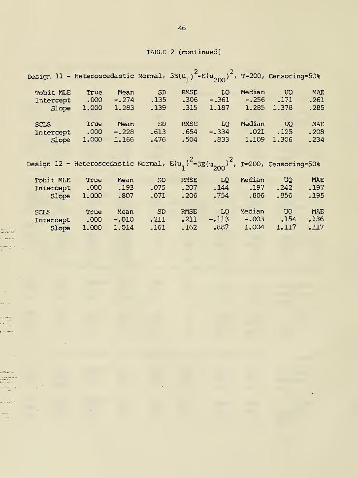
Designs 11 and 12 make the scale of the error terms a linear function of
x'P , while maintaining an overall variance T J E(u ) of unity. For theseX ^
designs, the "relative scale" is the ratio of the standard deviation of the
2 2200th observation to the first (e.g., in design 11, E(u2qq) =3E(u. ) ). With
increasing heteroscedasticity (design 11), most of the error variability is
associated with positive i|P_ values, and the SCLS estimator performs
relatively poorly; for decreasing heteroscedasticity (design 12), this
conclusion is reversed. In both of these designs, the bias of the Gaussian
MLE is much more pronounced, suggesting that failure of the homoscedasticity
assimiption may have more serious consequences than failure of Gaussianity in
censored regression models.
While the results in Table 2 are not unambiguous with respect to the
relative merits of the SCLS estimator to the misspecified KLE, there is
reason to beleive that, for practical purposes, the foregoing results present
an overly-favorable picture of the performance of the Gaussian MLE. As Ruud
[1984 J notes, more substantial biases of misspecified maximum likelihood
estimation result when the joint distribution of the regressors is
asymmetric, with low and high values of xlp being associated with different
components of the z. vector. The designs in Table 2, which were based upon a
single symmetrically distributed covariate, do not allow for this source of
bias, which is likely to be important in empirical applications.
In any case, the performance of the symmetrically censored least
squares estimator is much better than that of a two-step estimator (based
upon a normality assumption) which uses only those observations with y^ >
in the second step. A simulation study by Paarsch [1984], which used designs
very similar to those used here, found a substantial efficiency loss of this
two-step estimator relative to Gaussian maximum likelihood. In terms of both
relative efficiency and comutational ease, then, the symmetrically censored
least squares estimator is preferable to this two-step procedure.
5. Extensions and Limitations
The "symmetric trimming" approach to estimation of Tobit models can be
generalized in a number of respects. An obvious extension would be to permit
more general loss functions than squared error loss. That is, suppose p{K) is a
symmetric, convex loss function which is strictly convex at zero; then for the
truncated regression model, the analogue to Em (P ) of (2.7) would be
"^
.1
(5.1) Rj(P; p) = I p(y^ - max{-^ y^, x^p})
2which reduces to EmCP) when p(X) = X . A similar analogue to S^(p) of (2.10) is
T .
(5.2) Sj(P; p) = I p(y^ - min{ly^, x^p} )
X"" I
T
It=1
T /
+ I 1(y^ > 2x;P)Lp(-2 y^) - p(max{0, x^.?})].
When p(X) = |X|, the minimand in (5*2) reduces to the objective function which
defines the censored LAD estimator,
T
(5.3) Sm(P; LAD) = I ly+ - max{0, xlp}|
;
t=1 ^ ^
under somewhat different conditions (which did not require symmetry of the error
distribution), the corresponding estimator was shown in Powell [1984 J to be
consistent and asymptoticallj'- normal. On the other hand, if the loss function
p{X) is twice continuously differentiable, then the results of Theorems 1 and 2
can be proved as well for the estimators minimizing (5 -2) and (5-1 ), with
q/appropriate modification of the asymptotic covariance matrices.—'
To a certain extent, the "symmetric trimming" approach can be extended to
other limited dependent variable models as well. The censored and truncated
regression models considered above presume that the dependent variable is known
to be censored (or truncated) to the left of zero. Such a sample selection
mechanism may be relevant in some econometric contexts (e.g., individual labor
supply or demand for a specific commodity), but there are other situations in
which the censoring (or truncation) point vrould vary with each individual. A
prominent example is the analysis of survival data; such data are often left-
truncated at the individual's age at the start of the study, and right censored
at the sum of the duration of the study and the individual's age when it begins.
The symmetrically trimmed estimators are easily adapted to limited dependent
variable models with known limit values. In the survival model described above,
let L. and D, be the lower truncation and upper censoring point for the t
observation, so that the dependent variable y, is generated from the model
(5.4) y^ = min{x^Pp + v^, U^} , t = 1, ..., T,
where v, has density function
(5.5) g,(x) H 1 (X > L^ - x;p^)f^(x)Lp,(L^ - x;p^)j-i, .
25
for F^(*) and f+(*) satisfying Assumption E2. The corresponding symmetrically
trimmed least squares estimator would minimize
(5.6) R*(P) ^ 1 l(x;P < -^(U^ + ^t^^^^t ~ ^^^^^t * ^t^' "^t^^^^X
-I l(x;p >^(U^^L^))(y^-mxn4(y^.U^), x;p}
X
.Ii(x;p >;(u^.L^)).i(;(y, ^u^x .;p)X
2-1
•[%(yt- U^))-" - (min{0, x;p - U^})^J
and consistency and asymptotic normality for this estimator could be proved using
appropriate modifications of the corresponding assumptions for p and p„.
In the model considered ahove, the upper and lower "cutoff" points U, and
L. are assxmed to he observable for each t; however, many limited dependentX
"variable models in use do not share this feature. In survival analysis, for
example, it is often assimed that the censoring point is observed only for those
data points which are in fact censored, on the grounds that, once an uncensored
observation occurs, the value of the "potential" cutoff point is no longer
relevant-!— As another example, a model commonly used in economics has a
censoring (truncation) mechanism which is not identical to the regression
equation of interest; in such a model (more properly termed a "sample selection"
model, since the range of the observed dependent variable is not necessarily
restricted), the complete data point (y^, z^) from the linear model
7^ = 2;^pp + u^ is observed only if some (unobserved) index function I, exceeds
26
zero, and the dependent variable is censored (or the data point is truncated)
otherwise. The index function I* is typicallj' written in linear form
I = zlct + e., depending upon observed regressors z., unobserved parameters a ,
t t t- Li
and an error term e, which is independent across t, but is neither independent ,
of, nor perfectly correlated with, the residual u, in the equation of interest.
Unfortunately, the "symmetric trimming" approach outlined in Section 2 does
not appear to extend to models with unobserved cutoff points. In the sample
selection model described above, only the sign of I. and not its value is
observed, so "symmetric trimming" of the sample is not feasible, since it is not
possible to determine whether I, < 2x!a , which is the trimming rule
corresponding to y. < 2xlp in the simpler Tobit models considered previously.
This example illustrates the difficulty of estimation of (a', p') in the model
with I, * y!? when the joint distribution of the error terms is unknown.—
'
Finally, the approach can naturally be extended to the nonlinear regression
model, i.e., one in which the linear regression function is h,(x,, P ). ¥ith
some additional regularity conditions on the form of h,(»)(such as
differentiability and uniform boundedness of moments of h.(') and IIBh./Spil over t
and B), the results of Theorems 1 through 4 should hold if "sip" and "x." are
replaced by "h,(z., p)" and "Bh./5p" throughout. Of course, just as in the
standard regression model, the symmetric trimming approach will not be robust to
misspecification of the regression fxmction h.(«); nonetheless, theoretical
considerations are more likely to suggest the paper form of the regression
function than the functional form of the error distribution in empirical
applications, so the approach proposed here addresses the more difficiilt of these
two specification problems.

27
APPENDIX
Proofs of Theorems in Text
Proof of Theorem 1
A
(j_) Strong Consistency ; The proof of consistency of P follows the approach of
Amemiya [''973 J and White [1980 J by showing that, in large samples, the objective
function S„ (p ) is minimized by a sequence of values which converge a.s. to p .
First, note that minimization of S^ (P ) is equivalent to minimiztion of theJ.
normalized function
(A.1) Q^(P) =^ [S^(P) - S^(P^)J,
which can be written more explicitly as
T
(A.2) Q^(P)H^ I {l4y^< min{2;p, x;p^})[(y^-z;p)^-(y^-x;p^)2j
- l(x;P < ^ y, < x;p^)[(^ yj2-(max{0, .;p})2 - ij^-.'^^f]
^ ^^^;po 4 ^t < -;p)L(yt-^p^' - ^1 ^/ ^ (--^°' -;Po>)'-'
•Dl^2 / r r\ ..to -1 n2 n .+ 1(-^ y^ > max{3:;.P,z^^})[(maz{0, z^p})^ - (maxlO, ^\^^)) \)
2ify inspection, each term in the simi is bounded by llz.ll (llpH + lip II ) , so by Lemma
X
2.3 of ¥hite Ll980j,
(A.3) liJD iQrp(P) - eLg^(P)J| =
uniformly in p B by the compactness of B. Since E[q„(P )J = 0, p will be
strongly consistent if, for any e > 0, E[Q^(P)J is strictly greater than zero
uniformly in P for np - p H > e and all T sufficiently large, by Lemma 2.2 of
White [1980].
After some manipulations (which exploit the symmetry of the conditional
distribution of the errors), the conditional expectation of Qm(P) given the
regressors can be written as
(A.4) ELQj(P)1z^,...,XjJ
;J^{iK^<o<z;p)L4?p^Sx;p)2dF^(0
to
f^O
- 1(0 < 4P„ < x;p)L/!^Sz;6)2dF^(0
-sip +22:;p .p
t
29
to
-xlp +2x;p
to
^/-x;p .2.;p ^ L(x;6a;pj2(x.x;p^)2 - (x.x;p^-2x;p)2jdF^U)j}
to t
where
(A.5) 6 H p - p^
here and throughout the appendix, and where ^.(X) is the conditional c.d.f. of u,
given X.. All of the integrals in this expression are nonnegative, so
(A.6) ELQj(P)ki,...,X^J
X TO
^^-;po > ^' ^^ > -? > °)/!x-?^(^s)'Li-(Vx;p^)^jdF (o
to
^K^o^^o' -;p> -;Po)/!x;p K^)''^^^^^)^
where e is chosen as in Assumptions E and El. Without loss of generality, let
30
z^ = min{E^, Cq}; then, for any t: in (O, e^J,
(A. 7) ErQrj,(P) |x^,...,x,p]
S, ,2
^0 2,, ,, , s2.^(^;Po >
^o' ^;Po > ^P > o)i(u;6| > o/o" Tni-(xA^)'Jt^dx
"o „ 2
t
linally, let K = |- e^(K)5/2(4-^t))^
^^^ j. (jg^^ned in Assumption R. Then taking
expectations with respect to the distribution of the regressors and applying
Holder's and Jensen's inequalities yields
(A.8) e[Qt,(P)]
X
> Kx^ 1 I ELi (z;P^ > e^)-1 ( ix;6| > t)IIx^Ii2J^
X
31
> Ki^i^l eLi(x;p^ > E^)-i(|x;6| > r)(x;6)2|i6ir2j}5
where v™, the smallest characteristic root of the matrix N„, is bounded below by
V for large T by Assumption R. Thus, whenever II 6 II lip - p H > e, choosing x soo o
that T < V E shows that E[Qn,(P)J is uniformly bounded away from zero for all T
> T , as desired.
(ii) Asymptotic Normalit;y : The proofs of asymptotic normality here and below
are based on the approach of Huber fS^Tj, suitably modified to apply to the non-
identically distributed case. (For complete details of the modifications
required, the reader is referred to Appendix A of Powell [1984]). Define
(A.9) (I'di^, x^, p) 2 l(x;.p > 0)x^(min{y^, 2x^p} - x^p)
= 1 (z^p > 0)x^(nin{max{u^ - x^5, -2;^p} , x^p} );
then Ruber's argument requires that
(A.10) ^ I 4,(u^, x^, p^) = 0^(1).
But the left-hand side of (A. 10), multiplied by -2 /t", is the gradient of the
objective function S^ (P ) defining P„s so it is equal to the zero vector for large
32
T by Assumption P and the strong consistency of P„.
Other conditions for application of Ruber's argument involve the quantities
^.(P, d) = sup Hiu., X., p) - (|;(u^, X,, y)'I
^ llp-ylKd ^ ^ ^ ^
and
^rp(P) - T ^ EL'i'U^, x^, P)J.
Aside from some technical conditions which are easily verified in this situation
(such as the measurability of the {|i^}), Ruber's argument is valid if the first
two moments of \i^ are 0(d), and X^(p) > a lip - p^ll (some a > O), for all p near
P , d near zero, and T > T .
Simple algebraic manipulations show that
(A. 11) ^^(P, d) = -sup lll(x^p > 0)x^(nin{y^ - x;.p , x^p} )
Hp-ylld
1 (x^Y > 0)z^(min{y^ - x'^y , x^y} )ll
< llx^ll^d,
so that
(A.12) eLh^(P, d)J < k//(4-t,)^^
ELh,(P, d)j2 <K//(4-^)d2.
so both are 0(d) for d near zero. Furthermore,
(A.13) >.j(p) = -Cj(p - p^) + o(iip . p^n^),
53
where C™ is the matrix defined in the statement of tne theorem. This holds
because
(A.14) i^^^i^) + Cy(p - p^)ll
X O
f^o f^ x.p
t to
<E 41 l(|x;pj < |x;6i)x^{/'^rp'''^^*^-xl6)dFJX)X o
t ' t
X X
X X X
< 4L^E nl I L^^(x;6)2jll
< 4L (K)V(4+Ti) „2„2_00
Thus Xj(p)«np - P^^ll" > a > for all p in a suitably small neighborhood of p ,
since C™ is positive definite for large T by Assumption E and E1 . The argimient
54
leading to Ruber's [I957j Lemma 3 thus yields the asymptotic relation
(A.15) V r^%- Po^ = /tI '^K' -t' Po^ ' %^'^'
Application of the Liapunov form of the central limit theorem yields the result,
where the covariance matrix is calculated in the usual way.
Proof of Theorem 2:
(i) Strong Consistency : The argument is the same as for Theorem 1 above; strong
consistency of P^ holds if p uniquely minimizes T"^e[r^(P) - IL, (P )] = e[m_(P)J
uniformly in P for T sufficiently large. By some tedious algebra, it can be
shown that the following inequality holds:
(A.16) ELMj(p)lz^,...,ZyJ
> T I ^4F,(x;p^)j-^{i(x;p^ > 0, .;p < o)j"/\U'j^-xf - x^jdF^a)
x'6Ks^p^ < 0, x\p > o)/q* L(3c;p-x)^ - ).^JdF^(\)
i(r;p^ > 0, z;p > o)J^^^ L(k;6|-\)^ - x^jdp^(\)},
55
Using the conditions m E2, it can be shown that, by choosing: t sufficiently-
close to zero,
(A.17) eLk^(p)J > T^LhCj) - h(^)J il ELi(x;p^ > t^).l(|x;5| > t)J,
which corresponds to inequality (A. 7) above. The same reasoning as in (A. 8) thus
shows that ELKj(P)J > uniformly in p for lip - p^H > e and T > T^^ , as desired.
(ii) Asymptotic formality : The proof here again follows that in Theorem 1 ; in
this case, defining
(A.18) 4.(v^, x^, P) = l(y^ < 2x:p)(y^ - x;p)x^
the condition
(A.19) ^ I (^(v^, x^, pj) = 0p(l)
must again be established; but the left-hand side of (A.I 9)? multiplied by -2 /T,
is the (left) derivative of the objective function Em(P) evaluated at p„, so
(a. 19) can be established using the facts that p_ minimizes E_ (P ) and that the
fiistribution of v. continuous (a similar argument is given for Lemma A. 2 of
Ruppert and Carroll Ll980j).
56
For this problem, the appropriate quantities J^+(P, d) and X^^i?) can be shown
to satisfy
(A. 20) ^^(p, d) < ^I llx^^d
and
(A.21 ) II\^(P) + (W^ - V^)(p - P^)ll = 0(llp - P^I|2)
for p near p , so
1
(A.22) (Wj - Vj)/T(P - P^) = ^ I (|.(v^ , x^ , |) + Op(l )
as before, and application of Liapunov's central limit theorem yields the result.
Proof of Theorem 3:
Only the consistency of D„ will be demonstrated here; consistency of C„ can
Abe shown in an analogous way. First, note that !)„, is asymptotically equivalent
to the matriz
(A.23) A^ = ^ I l(x;p^ > 0)-min{u2, ix\p ^)^}x^x'^;
X
that is, each element of the difference matriz r_ - A_ converges to zero almost
surely. This holds since, defining 6 = p - p , the (i,j) element of the
difference satisfies
37
(A. 24) |[Et - ^T^ij'
-^I K^P, > 0)niin{u2, (-;P,)^}x,,x .J
<1I1(KP,I < K^DL^P,)^^ K^T^'JI^it^^t
4? ^K^o ^ K^tI)-^^I^I < ^Po^^-^^K^t) ^ K^T^'jl^it^;it
A.
** 2
-^I iu;p, > K^D-iHuJ > x;p^)L-2(x;p^)(x;6^) ^ {.•6^)^}h.^..^
< I J Ilz^ll'^ll6j0(llp^ll + I16„II).
But since Ellz, D''^ is imiformly bounded, these terms converge to zero almost
XA A
surely by the strong consistency of Pm* Consistency of Dm then follows from the
almost sure convergence of A„ - e[a_,J = Arp - D„ to zero by Markov's strong law of
large numbers.
Proof of Theorem 4 :
Again, strong consistency of ¥ and Z^ can be demonstrated in the same way
A"it was shown for I)™ in the preceeding proof. To prove consistency of ¥„» it will
3S
first be shown that V is asynptotically equivalent to
(A.25) r^^I i(x;p^> o)(x;p^)x^x;.c-^Li(y, < cj ^ 1(0 < y,-2x;p^ < c^)j,
~ ~ ~ ~ pFirst, note that (c^/c^)V is asymptotically equivalent to V , since (c^''c_) ->• 1;
next, note that each element of (cn,/Cn,)V_ - T satisfies
(A.26) IL(c^/cj)Vj - r^J..
,2-1
X
X
<ll hz^ii^ c-^ni^n ^ 1 J iiz^ii^op^iic-^i (|v^+ x;p^-c„| < 0^-0^(1))X X
+ ^I »2^ll5lip^Ilc-1.l(iv^.z;p^-Cj| < CjLo (1) + c-^ll6jO llz^nj),
39
where 6 = P^ - P • Chebvshev's inequality and the fact that /T(P^ - P ) = o (1 )
can thus be used to show that the difference between V and T converges to zero
in probability.
Hie expected value of T is
(A.27) E[r^ = E{E[r^|x^,...,x^]}
E[-^I i(x;p^ > o)(x;p^)x^x;[F^(x;p^)rV'^ c-;f,(>. - .;^^)dx]
E[-il i(x;p^ > o)(x;p^)x^z;[F^(x;p^)]-VV,(c^ - x;6^)dx]
= Vj+ 0(1)
by dominated convergence, while
(A.28) Var([r^.^)
X
. 1(0< v^.x'^^< c^)]}
BO each element of T - V converges to zero in quadratic mean.
40
Density of
xle + V.to t
t*^o t
xle 2x13t^o t^o
FIGUEE 1
Density Function of y. in Truncated
and "Symmetrically Truncated" Sample
41
Density of
\^o ' \
Pr{y^ > 2x;6^}
S^ " ^t
zip 2z;eto to
FIGURE 2
Distribution of y. in Censored andX
"^TEunetrically Censored" Sample
42
Density of
to t
x;ti to
Density of
to t
zie 2z:eto to
FIGURE 3
Density of y in Bimodal
and Uniform Cases.
43
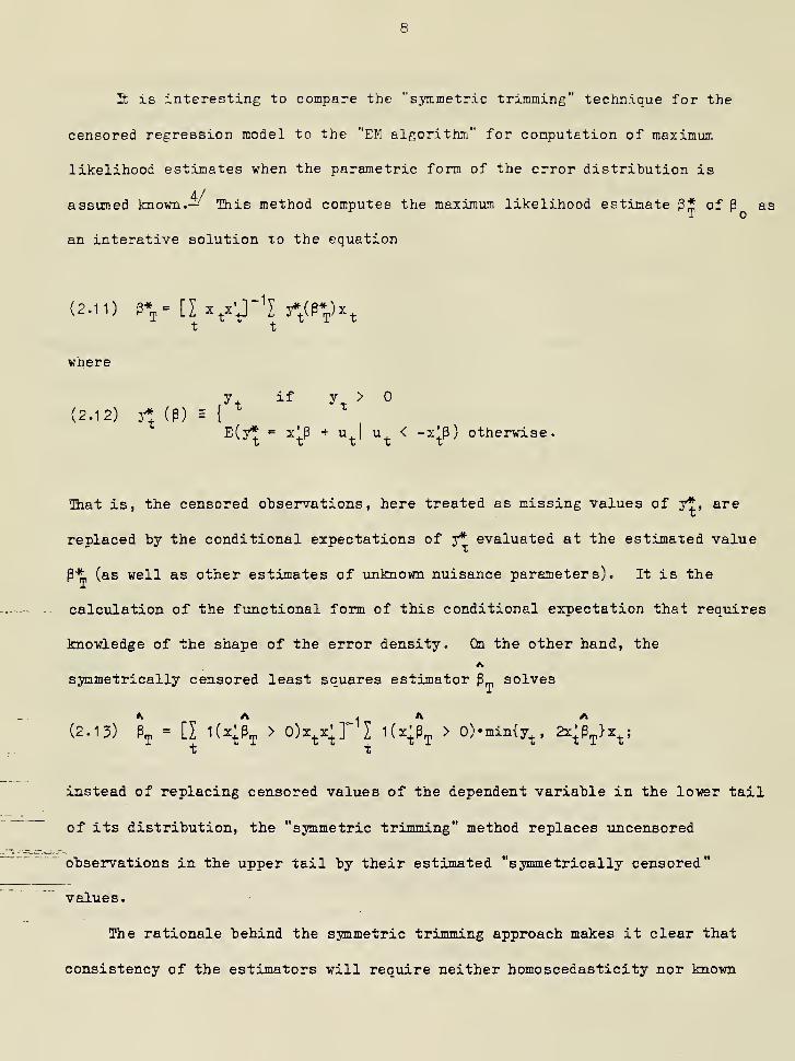
TABLE 1
Results of Simulations for Designs With Homocedastic Gaussian Errors
Design 1 - Scale=l, T=200, Censoring=50%
Tobit MLEIntercept
Slope
True.000
1.000
Mean-.0051.003
SD.093.097
RMSE.093.097
LQ-.071.934
Median.008
1.000
UQ.065
1.053
MAE.069.063
SCLSIntercept
Slope
True.000
1.000
Mean-.0801.060
SD.411
.325
RMSE.418
.331
LQ-.135.844
Median.028
.988
UQ.145
1.182
MAE.167
.171
Design 2 - Scale=l, T=100, Censoring=50%
Tobit MLEIntercept
Slope
SCLSIntercept
Slope
True Mean.000 -.001
1.000 1.009
True.000
1.000
Mean-.1291.101
SD RMSE.142 .142
.141 .142
SD RMSE.566 .580
.463 .474
LQ Median UQ MAE.088 .008 .109 .102.903 .994 1.108 .102
LQ Median UQ MAE.300 .074 .233 .263.780 .994 1.252 .273
Design 3 - Scale=2, T=200, Censoring=50%
Tobit MLEIntercept
Slope
SCLSIntercept
Slope
True Mean.000 -.011
1.000 .987
True Mean.000 -.903
1.000 1.622
SD RMSE LQ.194 .195 -.135
.161 .162 .875
SD RMSE LQ2.974 3.108 -.8211.887 1.987 .847
Median UQ MAE.012 .145 .141
.980 1.100 .117
Median UQ MAE-.079 .208 .3111.132 1.665 .342
Design 4 - Scale=l, T=200, Censoring=25%
Tobit MT.E True Mean SD RMSE LQ Median UQ MAEIntercept 1.000 .999 .080 .080 .949 1.000 1.046 .050
Slope 1.000 1.002 .077 .077 .946 1.003 1.055 .054
SCLS True Mean SD RMSE LQ Median UQ MAEIntercept 1.000 .981 .123 .124 .919 .997 1.063 .072
Slope 1.000 1.019 .126 .128 .928 1.016 1.096 .085
44
TABLE 1 (continued)
Design 5 - Scale=l, T=200, Censoring=50%, Two Slope Coefficients
Tobit MLE True Mean SD RMSE LQ Median UQ MAEIntercept .000 -.001 .102 .102 -.067 .004 .077 .069
Slope 1 1.000 .996 .095 .095 .942 .995 1.056 .057Slope 2 .000 -.011 .083 .084 -.071 -.011 .045 .062
SCLS True Mean SD RMSE LQ Median UQ MAEIntercept .000 -.174 .497 .527 -.322 -.023 .129 .200
Slope 1 1.000 1.124 .380 .399 .878 1.042 1.256 .193Slope 2 .000 -.015 .128 .129 -.098 -.015 .064 .080
Design 6 - Scale=l/ T=300, Censoring=50%, Two Slope Coefficients
Tobit MLE True Mean SD RMSE LQ Median UQ MAEIntercept .000 -.002 .082 .082 -.056 .008 .055 .056
Slope 1 1.000 .998 .083 .083 .940 .996 1.055 .059
Slope 2 .000 .003 .066 .066 .-.037 .003 .041 .040
SCLS True Mean SD RMSE LQ Median UQ MAEIntercept .000 -.120 .407 .425 -.252 -.011 .117 .160
Slope 1 1.000 1.086 .315 .326 .897 1.020 1.222 .146Slope 2 .000 .002 .094 .094 -.058 .004 .061 .058
45
TABLE 2
Results of Simulations for Designs Without Homocedastic Gaussian Errors
Design 7 - Laplace/ T=200, Censoring=50%
Tobit MLEIntercept
Slope
True.000
1.000
Mean-.0371.052
SD.101.109
RMSE.108
.121
LQ-.102.974
Median-.0321.047
UQ.032
1.125
MAE.071.081
SCLSIntercept
Slope
True.000
1.000
Mean-.0331.034
SD.203
.197
RMSE.205
.200
LQ-.148.894
Median.018
1.005
UQ.110
1.168
MAE.122
.129
Design 8 - Std. Cauchy, T=200, Censoring=50%
Tobit MLE True Mean SD RMSE LQ Median UQ MAEIntercept .000 -29.506 183.108 185.470 -10.522 -4.333 -2.045 4.422
Slope 1.000 25.826 166.976 168.812 2.559 4.241 7.768 3.241
SCLS True Mean SD RMSE LQ Median UQ MAEIntercept .000 -.352 1.588 1.626 -.404 -.002 .185 .248
Slope 1.000 1.439 2.537 2.575 .834 1.052 1.353 .240
Design 9 - Normal Mixture; Relative Scale=4, T=200, Censoring:=50%
Tobit MLE True Mean SD RMSE LQ Median UQ MAEIntercept .000 -.065 .098 .118 -.126 -.052 .005 .072
Slope 1.000 1.087 .124 .152 .999 1.074 1.161 .095
SCLS True Mean SD RMSE LQ Median UQ MAEIntercept .000 -.013 .215 .215 -.122 .024 .130 .130
Slope 1.000 1.019 .191 .192 .896 1.001 1.123 .110
Design 10 - Normal Mixture, Relative Scale=9/ T=200, Censoring=50%
Tobit MLE True Mean SD RMSE LQ Median UQ MAEIntercept .000 -.180 .125 .219 -.237 -.159 -.086 .160
Slope 1.000 1.194 .166 .255 1.078 1.174 1.268 .174
SCLS True Mean SD RMSE LQ Median UQ MAEIntercept .000 -.020 .108 .110 -.082 -.007 .054 .066
Slope 1.000 1.019 .118 .120 .936 1.009 1.092 .069
46
TABLE 2 (continuec3)
2 2Design 11 - Heterosceciastic Normal, 3E(u ) =E(u ) , T=200, Censoring=50%
Tobit MLEIntercept
Slope
SCLSIntercept
SloE>e
True Mean.000 -.274
1.000 1.283
True Mean.000 -.228
1.000 1.166
SD RMSE LQ.135 .306 -.361
.139 .315 1.187
SD RMSE LQ.613 .654 -.334.476 .504 .833
Mecaian UQ MAE-.256 .171 .2611.285 1.378 .285
Median UQ MAE.021 .125 .208
1.109 1.306 .234
2 2Design 12 - Heteroscedastic Normal, E(u ) =3E(u ) , T=200, Censoring=50%
Tobit MLEIntercept
Slope
True.000
1.000
Mean.193.807
SD.075
.071
RMSE.207
.206
LQ.144.754
Median.197
.806
UQ.242.856
MAE.197.195
SCLSIntercept
Slope
True.000
1.000
Mean-.0101.014
SD.211
.161
RMSE.211
.162
LQ-.113,887
Median-.0031.004
UQ.154
1.117
MAE.136
.117
47
roOTNOTES
1/ This research was supported by National Science Foundation Grants No.
SES79-12965 and SES79-13976 at Stanford University and SES83-09292 at the
Massachusetts Institute of Technology. I would like to thank T. Amemiya,
T. W. Anderson; T. Bresnahan, C. Cameron/ J. Hausman, T. MaCurdy,
D. McFadden, W. Newey, J. Rotemberg, P. Ruud/ T. Stoker/ R. Turner, and a
referee for their helpful comments.
2/ These references are by no means exhaustive; alternative estimation
methods are given by Kalbfleisch and Prentice [1980], Koul, Suslara, and
Van Ryzin [1981], and Ruud [1983], among others..
3/ Since the right-hand side of (2.6) is discontinuous, it nay not be possible
to find a value of B which sets it to zero for a particular sample. In the
asymptotic theory to follow, it is sufficient for the summation in (2.6),
Lon6^
-1/2
when normalized by — and evaluated at the proposed solution g / to converge
to the zero vector in probability at a faster rate than T
4/ A more detailed discussion of the EM algorithm is given by Dempster, Laird,
and Ri±)in [1977].
5/ If C and D„ have limits C and D , then result (ii) can be written in the— T T CO 00
more familiar form T(B„ - 6 ) ->- N(0, CDC ).'
»J>Q * ' CO 00 00 '
48
6/ The scaling sequence c_, niay depend/ for example/ upon some concomittant
estimate of the scale of the residuals.
7/ Turner [1983] has applied symmetrically censored least squares estiiretion
to data on the share of fringe benefits in labor compensation. The
successive approximation formula (2.13) was used iteratively to compute the
regression coefficients/ and standard errors were obtained using ^ and D .
above. The resulting estimates/ while generally of the same sign as the
maximum likelihood estimates assuming Gaussian errors, differed
substantially in their relative magnitudes, indicating failure of the
assumptions of normality or homoscedasticity.
8/ Gaussian deviates were generated by the sine-cosine transform, as applied
-'-- to uniform deviates generated by a linear congruential scheme; deviates
-' for the other error distributions below were generated by the
inverse-transform method. The symmetrically censored least squares
- estimator was calculated throughout using (2.13) as a recursion formula,
with classical least squares estimates as starting values. The Tobit '
maximum likelihood estimates used the Newton-Raphson iteration, again with
least squares as starting values.
9/ Of course, if the loss function 'p{') is not scale equivariant, some
concommitant estimate of scale may be needed, conplicating the asynptotic
theory.
49
10/ This argument is somewhat more compelling in the case of an i.i.d.
dependent variable than in the regression context/ where conditioning on
the censoring points is similar to conditioning on the observed values of
the regressors. In practice » even if the data do not include censoring
values for the uncensored observations/ such values can usually be imputed
as the potential survival time assuming the individual had lived to the
completion of the study.
11/ Cosslett [1984a] has recently proposed a consistent/ nonparametric two-step
estiirator of the general sample selection model/ but its large-sample
distribution is not yet known. Chamberlain [1984] and Cosslett [1984b]
have investigated the maximum attainable efficiency for selection models
when the error distribution is unknown.
50
REFERENCES
Amemiys/ T. [1973], "Regression Analysis When the Dependent Variable is
Truncated Normal," Econometrica , 41: 997-1016.
Arabmazar, A. and P. Schmidt [1981], "Further Evidence on the Robustness of
the Tobit Estittator to Heteroskedasticity, " Journal of Econometrics , 17:
253-258.
Arabmazar, A. and P. Schmidt [1982], "An Investigation of the Robustnessof the Tobit Estimator to Non-Normality," Econometrica , 50: 1055-1063.
Buckley, J. and I. James [1979], "Linear Regression with Censored Data,"Biometrika , 66: 429-436.
Chamberlain, G. [1984], "Asymptotic Efficiency in Semiparametric Models withCensoring," Department of Economics, University of Wisconsin-Madison,manuscript, May.
Cosslett, S.R. [1984a], "Distribution-Free Estimator of a Regression Modelwith Sample Selectivity," Center for Econometrics and Decision Sciences,University of Florida, manuscript, June.
Cosslett, S.R. [1984b], "Efficiency Bounds for Distribution-Free Estimators ofthe Binary Choice and Censored Regression Models," Center forEconometrics and Decision Sciences, University of Florida, manuscript,June.
Deiipster, A.P. , N.M. Laird, and D.B. Rubin [1977], "Maximum Likelihood fromIncomplete Data via the EM Algorithm, " Journal of the Royal StatisticalSociety , Series B , 39: 1-22.
Duncan, G.M. [1983], "A Robust Censored Regression Estimator", Department ofEconomics, Washington State University, Working Paper No. 581-3.
Efron, B. [1967], "The Two-Sample Problem with Censored Data," Proceedings ofthe Fifth Berkeley Symposium , 4: 831-853.
Eicker, F. [1967], "Limit Theorems for Regressions with Unequal and DependentErrors," Proceedings of the Fifth Berkeley Symposium , 1: 59-82.
Fernandez, L. [1983], "Non-parametric Maximum Likelihood Estimation ofCensored Regression Models," manuscript, Department of Economics,Oberlin College.
Goldberger, A.S. [1980], "Abnormal Selection Bias," Social Systems ResearchInstitute, University of Wisconsin-Madison, Workshop Paper No. 8006.
Hausman, J. A. [1978], "Specification Tests in Econometrics," Econometrica ,
46: 1251-1271.
Heckman, J. [1979], "Sample Bias as a Specification Error," Econometrica ,
47: 153-162.
51
Huber> P.J. [1965]/ "The Behaviour of Maximum Likelihood EstiiiBtes UnderNonstandard Conditions/" Proceedings of the Fifth Berkeley Symposium /
1: 221-233.
Hurd/ M. [1979]/ "Estimation in Truncated Samples When There is
Heteroskedasticity/ " Journal of Econometrics / 11: 247-258.
Kalbfleisch/ J.O. and R.L. Prentice [1980]/ The Statistical Analysis of
Failure Time Data / New York: John Wiley and Sons.
Koul/ H. ; Suslarla, V./ and J. Van Ryzin [1981]/ "Regression Analysis WithRandomly Right Censored Data/" Annals of Statistics / 9: 1276-1288.
Maddala/ G.S. and F.D. Nelson [1975]/ "Specification Errors in LimitedDependent Variable Models/" ttetional Bureau for Economic Research/
Working Paper No. 96.
Miller/ R. G. [1976]/ "Least Squares Regression With Censored Data/"
Biometrika / 63: 449-454.
Paarsch/ H.J. [1984]/ "A Monte Carlo Comparison of Estimators for Censored
Regression/" Annals of Econometrics / 24: 197-213.
Powell/ J.L. [1984]/ "Least Absolute Deviations Estimation for the Censored
Regression Model/" Journal of Econometrics / 25: 303-325.
Ruppert/ D. and R.J. Carroll [1980]/ "Trimmed Least Squares Estimation in the
Linear Model," Journal of the American Statistical Association / 75:
828-838.
Ruud/ P. A. [1983], "Consistent Estimation of Limited Dependent Variable ModelsDespite Misspecification of Distribution/" manuscript/ Department of
Economics, University of California, Berkeley.
Tobin, J. [1958], "Estimation of Relationships for Limited DependentVariables, " Econometrica , 26: 24-36.
Turner, R. [1983], The Effect of Taxes on the Form of Compensation , Ph.D.dissertation. Department of Economics, Massachusetts Institute ofTechnology.
White/ H. [1980], "A Heteroskedasticity-Consistent Covariance MatrixEstimator and a Direct Test for Heteroskedasticity," Econometrica ,
48: 817-838.
K
950ii 0/+6

MIT LIBRARIES
3 TDflD DD3 DhE 053

»<•(
> i k{i *
•fc*^
il»l
0f¥-hi
^?^^'#.«•. tA*
5\>
-* 1
./
-j?<
^ji'f'j
m

Date Due

Idcpt- Goi^ /^ on y^<ck c^^^r-