441
Symmetries and Curvature Structure in General Relativity
World Scientific Lecture Notes in Physics
Published Vol. 49: Field Theory, Disorder and Simulations
G Parisi Vol. 50: The Quark Structure of Matter
M Jacob Vol. 51 : Selected Topics on the General Properties of Quantum Field Theory
F Strocchi Vol. 52: Field Theory: A Path Integral Approach
A Das Vol. 53: Introduction to Nonlinear Dynamics for Physicists
H D I Abarbanel, et al.
Vol. 54: Introduction to the Theory of Spin Glasses and Neural Networks V Dotsenko
Vol. 55: Lectures in Particle Physics D Green
Vol. 56: Chaos and Gauge Field Theory T S Biro, et al.
Vol. 57: Foundations of Quantum Chromodynamics (2nd ed.) T Muta
Vol. 59: Lattice Gauge Theories: An Introduction (2nd ed.) H J Rothe
Vol. 60: Massive Neutrinos in Physics and Astrophysics R N Mohapatra and P B Pal
Vol. 61 : Modern Differential Geometry for Physicists (2nd ed.) C J lsham
Vol. 62: ITEP Lectures on Particle Physics and Field Theory (In 2 Volumes) M A Shifman
Vol. 64: Fluctuations and Localization in Mesoscopic Electron Systems M Janssen
Vol. 65: Universal Fluctuations: The Phenomenology of Hadronic Matter R Botet and M Ploszajczak
Vol. 66: Microcanonical Thermodynamics: Phase Transitions in “Small” Systems D H E Gross
Vol. 67: Quantum Scaling in Many-Body Systems M A Continentino
Vol. 69: Deparametrization and Path Integral Quantization of Cosmological Models C Simeone
Vol. 70: Noise Sustained Patterns Markus Loecher
Vol. 73: The Elmentary Process of Bremsstrahlung W. Nakel and E. Haug
Symmetries and Cuwa ture Structure in General Relativity
G S Hall University of Aberdeen, UK
K World Scientific N E W JERSEY * LONDON - SINGAPORE - BElJlNG - S H A N G H A I - HONG KONG - TAIPEI * C H E N N A I
Published by
World Scientific Publishing Co. Pte. Ltd. 5 Toh Tuck Link, Singapore 596224 USA office: Suite 202,1060 Main Street, River Edge, NJ 07661 CJK office: 57 Shelton Street, Covent Garden, London WC2H 9HE
British Library Cataloguing-in-Publication Data A catalogue record for this book is available from the British Library.
SYMMETRIES AND CURVATURE STRUCTURE IN GENERAL RELATIVITY
Copyright 0 2004 by World Scientific Publishing Co. Re. Ltd. All rights reserved. This book, or parts thereoj may not be reproduced in any form or by any means, electronic or mechanical, including photocopying, recording or any information storage and retrieval system now known or to be invented, without written permission from the Publisher.
For photocopying of material in this volume, please pay a copying fee through the Copyright Clearance Center, Inc., 222 Rosewood Drive, Danvers, MA 01923, USA. In this case permission to photocopy is not required from the publisher.
ISBN 981-02-1051-5
Printed in Singapore
Preface
A significant amount of relativistic literature has, in the past few decades, been devoted to the study of symmetries in general relativity. This book attempts to collect together the theoretical aspects of this work into some- thing like a coherent whole. However, it should be stressed that it is not a textbook on those exact solutions of Einstein’s equations which exhibit such symmetries; an excellent text covering these topics already exists in the literature. It is essentially a study of certain aspects of 4-dimensional Lorentzian differential geometry, but directed towards the special require- ments of Einstein’s general theory of relativity. Its main objective is to present a mathematical approach to symmetries and to the related topic of the connection and curvature structure of space-time and to pay atten- tion to certain problems which arise and which worry mathematicians more than physicists. It is also hoped that certain of the chapters, for example those on manifold theory and holonomy groups, may serve as more or less self contained introductions to these important subjects.
The book arose out of many years work with my research students in the University of Aberdeen and I thus wish to record my gratitude to M.S. Capocci, W.J. Cormack, J. da Costa, R.F. Crade, B.M. Haddow, Hassan Alam, C.G. Hewitt, A.D. Hossack, S. Khan, M. Krauss, W. Kay, M. Lampe, D.P. Lonie, D.J. Low, L.E.K. MacNay, N.M. Palfreyman, M.T. Patel, M.P. Ramos, A.D. Rendall, M. Robertson, I.M. Roy, G. Shabbir, J.D. Steele, J. Sun, J.D. Whiteley and the late D. Negm. I would also like to thank the many friends and colleagues, both in the University of Aberdeen and elsewhere, who contributed in one way or another to the preparation of this book and, in particular, D. Alexeevski, A. Barnes, P. Bueken, J. Carot, M.C. Crabb, S. Hildebrandt, C.B.G. McIntosh, M. Sharif, Ibohal Singh, I.H. Thomson, E.H. Hall, S. Munro and the late C. Gilbert.
v
vi Symmetries and Curvature Structure in General Relativity
Finally I wish to record my sincere thanks to John Pulham, whose con- versations on mathematics and physics and help in preparing this book have left me with a debt I can never repay, to Louise Thomson for her ex- cellent typing of most of the manuscript, to the World Scientific Publishing Company for their infinite patience and to Aileen Sylvester for her unselfish understanding and support.
Contents
Preface V
1 . Introduction 1
1.1 Geometry and Physics . . . . . . . . . . . . . . . . . . . . . 1 1.2 Preview of Future Chapters . . . . . . . . . . . . . . . . . . 5
2 . Algebraic Concepts 11
2.1 Introduction . . . . . . . . . . . . . . . . . . . . . . . . . . . 11 2.2 Groups . . . . . . . . . . . . . . . . . . . . . . . . . . . . . . 11 2.3 Vector Spaces . . . . . . . . . . . . . . . . . . . . . . . . . . 15 2.4 Dual Spaces . . . . . . . . . . . . . . . . . . . . . . . . . . . 22 2.5 Forms and Inner Products . . . . . . . . . . . . . . . . . . . 23
2.7 Lie Algebras . . . . . . . . . . . . . . . . . . . . . . . . . . . 38 2.6 Similarity, Jordan Canonical Forms and Segre Types . . . . 28
3 . Topology 41
3.1 Introduction . . . . . . . . . . . . . . . . . . . . . . . . . . . 41 3.2 Metric Spaces . . . . . . . . . . . . . . . . . . . . . . . . . . 42 3.3 Topological Spaces . . . . . . . . . . . . . . . . . . . . . . . 45
3.5 Subspace Topology . . . . . . . . . . . . . . . . . . . . . . . 51 3.6 Quotient Spaces . . . . . . . . . . . . . . . . . . . . . . . . 52 3.7 Product Spaces . . . . . . . . . . . . . . . . . . . . . . . . . 53 3.8 Compactness and Paracompactness . . . . . . . . . . . . . . 3.9 Connected Spaces . . . . . . . . . . . . . . . . . . . . . . . . 56 3.10 Covering Spaces and the Fundamental Group . . . . . . . .
. . . . . . . . . . . . . . . . . . . . . . . . . . . . . . 3.4 Bases 49
53
58
vii
viii Symmetries and Curvature Structure in General Relativity
3.11 The Rank Theorems . . . . . . . . . . . . . . . . . . . . . . 61
4 . Manifold Theory 63
4.1 Introduction . . . . . . . . . . . . . . . . . . . . . . . . . . . 63 4.2 Calculus on Rn . . . . . . . . . . . . . . . . . . . . . . . . . 64 4.3 Manifolds . . . . . . . . . . . . . . . . . . . . . . . . . . . . 65 4.4 Functions on Manifolds . . . . . . . . . . . . . . . . . . . . 68 4.5 The Manifold Topology . . . . . . . . . . . . . . . . . . . . 70 4.6 The Tangent Space and Tangent Bundle . . . . . . . . . . . 73 4.7 Tensor Spaces and Tensor Bundles . . . . . . . . . . . . . . 75 4.8 Vector and Tensor Fields . . . . . . . . . . . . . . . . . . . . 77 4.9 Derived Maps and Pullbacks . . . . . . . . . . . . . . . . . 81 4.10 Integral Curves of Vector Fields . . . . . . . . . . . . . . . . 83 4.1 1 Submanifolds . . . . . . . . . . . . . . . . . . . . . . . . . . 85 4.12 Quotient Manifolds . . . . . . . . . . . . . . . . . . . . . . . 92 4.13 Distributions . . . . . . . . . . . . . . . . . . . . . . . . . . 92 4.14 Curves and Coverings . . . . . . . . . . . . . . . . . . . . . 97 4.15 Metrics on Manifolds . . . . . . . . . . . . . . . . . . . . . . 99 4.16 Linear Connections and Curvature . . . . . . . . . . . . . . 104 4.17 Grassmann and Stiefel Manifolds . . . . . . . . . . . . . . . 116
5 . Lie Groups 119
5.1 Topological Groups . . . . . . . . . . . . . . . . . . . . . . . 119 5.2 Lie Groups . . . . . . . . . . . . . . . . . . . . . . . . . . . 121 5.3 Lie Subgroups . . . . . . . . . . . . . . . . . . . . . . . . . . 122 5.4 Lie Algebras . . . . . . . . . . . . . . . . . . . . . . . . . . . 124
5.6 Transformation Groups . . . . . . . . . . . . . . . . . . . . 131 5.7 Lie Transformation Groups . . . . . . . . . . . . . . . . . . 131 5.8 Orbits and Isotropy Groups . . . . . . . . . . . . . . . . . . 133 5.9 Complete Vector Fields . . . . . . . . . . . . . . . . . . . . 135 5.10 Groups of Transformations . . . . . . . . . . . . . . . . . . 138 5.11 Local Group Actions . . . . . . . . . . . . . . . . . . . . . . 140 5.12 Lie Algebras of Vector Fields . . . . . . . . . . . . . . . . . 142 5.13 The Lie Derivative . . . . . . . . . . . . . . . . . . . . . . . 144
5.5 One Parameter Subgroups and the Exponential Map . . . . 127
6 . The Lorentz Group 147
6.1 Minkowski Space . . . . . . . . . . . . . . . . . . . . . . . . 147
Contents ix
6.2 The Lorentz Group . . . . . . . . . . . . . . . . . . . . . . 150 6.3 The Lorentz Group as a Lie Group . . . . . . . . . . . . . . 158 6.4 The Connected Lie Subgroups of the Lorentz Group . . . . 163
Space-Times and Algebraic Classification 169
7.1 Space-Times . . . . . . . . . . . . . . . . . . . . . . . . . . . 169 7.1.1 Electromagnetic fields . . . . . . . . . . . . . . . . . 171 7.1.2 Fluid Space-Times . . . . . . . . . . . . . . . . . . . 172 7.1.3 The Vacuum Case . . . . . . . . . . . . . . . . . . . 172
7.2 Bivectors and their Classification . . . . . . . . . . . . . . . 173 7.3 The Petrov Classification . . . . . . . . . . . . . . . . . . . 184 7.4 Alternative Approaches to the Petrov Classification . . . . . 191 7.5 The Classification of Second Order Symmetric Tensors . . . 202 7.6 The Anti-Self Dual Representation of Second Order
Symmetric Tensors . . . . . . . . . . . . . . . . . . . . . . . 208 7.7 Examples and Applications . . . . . . . . . . . . . . . . . . 215 7.8 The Local and Global Nature of Algebraic Classifications . 221
8 . Holonomy Groups and General Relativity 227
8.1 Introduction . . . . . . . . . . . . . . . . . . . . . . . . . . . 227 8.2 Holonomy Groups . . . . . . . . . . . . . . . . . . . . . . . 227 8.3 The Holonomy Group of a Space-Time . . . . . . . . . . . . 234 8.4 Vacuum Space-Times . . . . . . . . . . . . . . . . . . . . . . 245 8.5 Examples . . . . . . . . . . . . . . . . . . . . . . . . . . . . 248
9 . The Connection and Curvature Structure of Space-Time 255
9.1 Introduction . . . . . . . . . . . . . . . . . . . . . . . . . . . 255 9.2 Metric and Connection . . . . . . . . . . . . . . . . . . . . . 255 9.3 Metric, Connection and Curvature . . . . . . . . . . . . . . 259 9.4 Sectional Curvature . . . . . . . . . . . . . . . . . . . . . . 270 9.5 Retrospect . . . . . . . . . . . . . . . . . . . . . . . . . . . . 282
10 . Affine Vector Fields on Space-Time 285
10.1 General Aspects of Symmetries . . . . . . . . . . . . . . . . 285 10.2 Affine Vector Fields . . . . . . . . . . . . . . . . . . . . . . 287 10.3 Subalgebras of the Affine Algebra;
Isometries and Homotheties . . . . . . . . . . . . . . . . . . 291 10.4 Fixed Point Structure . . . . . . . . . . . . . . . . . . . . . 296
7
X Symmetries and Curvature Structure in General Relativity
10.5 Orbit Structure . . . . . . . . . . . . . . . . . . . . . . . . . 10.6 Space-Times admitting Proper Affine Vector Fields . . . . . 10.7 Examples and Summary . . . . . . . . . . . . . . . . . . . .
11 . Conformal Symmetry in Space-times
11.1 Conformal Vector Fields . . . . . . . . . . . . . . . . . . . . 11.2 Orbit Structure . . . . . . . . . . . . . . . . . . . . . . . . . 11.3 Fixed Point Structure . . . . . . . . . . . . . . . . . . . . . 11.4 Conformal Reduction of the Conformal Algebra . . . . . . . 11.5 Conformal Vector Fields in Vacuum Space-Times . . . . . .
11.7 Special Conformal Vector Fields 11.6 Other Examples . . . . . . . . . . . . . . . . . . . . . . . .
. . . . . . . . . . . . . . .
12 . Projective Symmetry in Space-times
12.1 Projective Vector Fields . . . . . . . . . . . . . . . . . . . . 12.2 General Theorems on Projective Vector Fields . . . . . . . . 12.3 Space-Times Admitting Projective Vector Fields . . . . . . 12.4 Special Projective Vector Fields . . . . . . . . . . . . . . . . 12.5 Projective Symmetry and Holonomy . . . . . . . . . . . . .
13 . Curvature Collineations
13.1 Introduction . . . . . . . . . . . . . . . . . . . . . . . . . . . 13.2 Curvature Collineations . . . . . . . . . . . . . . . . . . . . 13.3 Some Techniques for Curvature Collineations . . . . . . . . 13.4 Further Examples . . . . . . . . . . . . . . . . . . . . . . . .
Bibliography
311 323 333
341
341 345 349 352 358 359 363
371
371 375 381 389 391
397
397 397 400 408
413
Index 42 1

Chapter 1
Introduction
1.1 Geometry and Physics
The use of geometrical techniques in modelling physical problems goes back over two thousand years to the Greek civilisation. But for these people physics was a prisoner of geometry (not to mention of egocentricity) and, in particular, of the circle. So, for example, whilst the Ptolemaic geocentric model of the solar system was a powerful model for its time, the geometrical input was not only restricted by the knowledge and prejudices of the pe- riod, but provided only an arena in which physics took place. In this sense geometry was not part of the physics but merely a mathematical conve- nience for its description. In the scientific renaissance of the 16th century onwards the Greek dominance and prejudices were gradually eroded but even Copernicus still felt the need of the beloved circle and his heliocentric theory still needed epicycles. Not until Kepler came upon the scene was the circle finally dethroned when, by the introduction of eliptical orbits, he was able to explain all, and more, than Copernicus could, without the need of epicycles.
The Keplerian system, precisely stated, turns out to be equivalent to a model of the solar system of a Newtonian type based on the inverse square law attraction of a central force. This was one of the most outstand- ing achievements of Newtonian physics and the Kepler-Newton system has been the standard theory of the solar system ever since (the modifications arising from general relativity theory, although important theoretically, for example in the solving of the Mercury orbital problem, are minor in prac- tice). But even in Newtonian mechanics the geometry of Euclid was still dominant and provided the unquestioned background in. which all else took place.
1-
2 Symmetries and Curvature Strzlcture in General Relativity
The geometrical description of physics alluded to above has, however, a formal beauty in that it is perhaps to be considered remarkable that the Greek description of, for example, planetary events using one of the most important constructions in Euclidean geometry, the circle, gives a reasonably accurate picture of the solar system. The other important object in Euclid’s geometry, the straight line, can also be thought of as having a physical context in the following simple way. Consider the Euclidean plane R2 with its usual system of “straight” lines etc. Now let f be a bijective continuous map f : R2 + R2 (although continuity hardly matters here) and consider the set R2 now with the straight line structure understood to be the images of the original straight lines under f . Thus the straight lines in the new system are the subsets of R2 of the form f(L) for all straight lines L in the original system. This set with this new linear structure formed by taking across from the original in an obvious way the concepts of length, angle etc under f is mathematically indistinguishable from the original and constitutes a perfectly good model of Euclidean geometry. However, one can distinguish them physically by, for example, regarding the copy of R2 as a horizontal surface and appealing to Galileo’s law of inertia for free particles traversing this surface or to the paths of light beams crossing it (or, quite simply, to the lines of shortest distance measured by taut pieces of string held on the surface) to determine “straight lines”. Each of these would presumably single out, at least in a local sense,the original copy of Euclid’s geometry.
These examples may be considered early references to the interplay be- tween geometry and physics but their true significance was presumably not fully realised until Hilbert set Euclidean geometry in proper perspec- tive with his axiomatisation of this system (Gauss, Bolyai and Lobachevski having earlier confirmed the existence of alternative geometries). In this sense, these mathematicians played important roles in the understanding of physics.
Another example of the role of geometry in physics comes from the de- velopment in the 18th and 19th centuries of analytical mechanics and La- grangian techniques. The work of D’ Alembert, Euler, Lagrange, Hamilton and others cast the formulation of Newtonian mechanics into the geometry of the configuration space (or extended configuration space). From this, the calculus of variations, and the work of Riemann on differential geom- etry, Newtonian theory was in some sense “geometrised” by reformulating it in a setting of the Riemannian type. As a simple example, consider an n-particle system under a time independent conservative force described in
Introduction 3
the usual 3n-dimensional Euclidean (configuration) space. The Euclidean nature (metric) of this space can be thought of as derivable from the ki- netic energy of the unconstrained system in a standard way. Suppose now that a holonomic constraint is imposed on the system by restricting the particle to move on some subspace (submanifold) of the original Euclidean space. One could attempt the solve this problem by working in the sub- manifold of constraint. In doing so, this submanifold inherits a metric from the original Euclidean metric and which, in general, is no longer Eu- clidean but is rather a “curved metric” of the general type envisaged by Riemann. An elegant finale to the problem was then given by Routh’s re- duced Lagrangian (Routhian). The problem has in a sense been geometrised (and the constraint removed). Also the theory assumes a “generally co- variant” form since the original inertial frame structure has been replaced by “generalised coordinates”. A similar geometrisation occurs when one rewrites Maxwell’s equations in generally covariant form by changing the usual Maxwell equations, written in an inertial frame in special relativity, by replacing the Minkowski metric that arises there by some general metric and partial derivatives by covariant derivatives.
However, there is a criticism of the claim that this procedure has pro- gressed further with the geometrising of the problem than the earlier ex- amples discussed above. The geometry in these examples really entered the proceedings with the imposition of the original Euclidean structure (and, in the first example, before the constraints were introduced). Thus the geometrical structure was on the arena initially and is again merely a convenience (albeit a useful one) for the solution of the problem. Sim- ilar comments apply to the more sophisticated geometrical approaches to mechanics inaugurated by Jacobi and Cartan (the latter albeit after the ad- vent of Einstein’s general relativity). In this sense, the geometry was given a-priori and was not subject to any restrictions (“field equations”). Thus it invites the criticism that it can influence the physics without any reciprocal influence on itself and was subject to unfavourable philosophical scrutiny by amongst others, Berkeley 111 and Mach 121. Also the introduction of “absolute” variables such as the background Euclidean metric in classical mechanics and Maxwell theory (essentially Newton’s absolute space) seems to suggest that making a theory “covariant” is a rather trivial matter. One more or less writes down the theory in its original “Euclidean” form and then allows everything to transform as a tensor when moving to some other coordinate system. This problem was apparently first recognised by Kretchmann [3] and elaborated on by Anderson [4] and Trautmann [5 ] ) .

4 Symmetries and Curvature Stmcture an General Relativity
The advantage of general relativity is that it contains the space-time metric as a “dynamical” variable (to be determined by solving field equa- tions) and that it contains no such “absolute” variables (except one must, perhaps, concede that the imposition of zero torsion on the Levi-Civita connection derived from the space-time metric amounts to making the tor- sion an absolute variable in this theory [5 ] . In this stronger sense general relativity is “generally covariant” . On the other hand, Newtonian classical theory has an absolute space-time splitting into absolute space and abso- lute time together with privileged (inertial) observers and, in addition, a privileged frame in which the ether is at rest if classical electromagnetic theory is to be accomodated within it. Special relativity has an absolute space-time metric and privileged inertial observers whereas, for example, the “bimetric” and “tetrad” variants of Einstein’s theory have absolute variables in the form of a flat metric [6] or a privileged tetrad system [7], respectively. Classical theory with its concept of force has to be able to distinguish between “real” forces (e.g. the gravitational attraction of one body on another) and the so called “fictitious” (accelerative) forces which arise in non-inertial frames. The ability to distinguish between these types of force is essentially the ability to distinguish between inertial and non- inertial frames. Newton’s theory claims each of these abilities (and thus introduces absolute variables) and Einstein’s claims neither. Thus there are no a priori distinguished reference frames (coordinate systems) in gen- eral relativity (although there are, of course, convenient ones!) and no concept of force (beyond that required in order to describe situations in relativity theory using Newtonian language!) Such remarks as these go un- der the name of the principal of covariance and its role in the foundations of general relativity is by no means agreed upon. A related (and also con- tentious) issue is the principle of equivalence. In its strong form it advocates the (local) indistinguishability of a gravitational field and an appropriately chosen acceleration field, In its weaker form it simply reiterates the results of the Eotvos type experiments thus effectively saying that there is a unique symmetric connection in space-time for determining space-time paths (this latter statement leaving room for curvature coupling terms). These topics will not be discussed any further here except to say that they can be used to suggest that a theory of gravitation could be based on a 4-dimensional manifold and whose dynamical variable is a metric of Lorentz signature which is determined by field equations of a tensorial nature. Such a theory is Einstein’ general relativity and it will be accepted, henceforth, without question.
Introduction 5
Einstein’s general theory of relativity is the most successful theory of the gravitational field so far proposed. It describes the gravitational field by a mathematical object called a space-time and is formalised as a pair ( M , g) where M is a certain type of 4-dimensional manifold (see chapter 7) and g is a Lorentz metric on M . The metric g together with its connec- tion and curvature “represent” the gravitational field. The restrictions on g are the Einstein field equations (together with boundary and other ini- tial conditions) and are ten second order partial differential equations for g. Since the theory was first published in 1916, it has progressed through early uncertain beginnings, when it played second fiddle to quantum the- ory and suffered from the “cosmological time problem” (until the latter’s correction), to a renaissance in the last fifty years. The problem of the lack of exact solutions to Einstein’s field equations has, to some extent, been overcome. In addition, the theory has been put on a much sounder footing both mathematically and physically.
1.2 Preview of Future Chapters
This book is not a text book on general relativity. There are numerous ex- cellent such texts available and thus no point in further duplication. Rather, it concentrates first on the topics of the connection and curvature struc- ture of space-times and then, later, on the various symmetries that are commonly studied in Einstein’s theory. In spite of this, an attempt will be made to make the book in some restricted sense, self-contained and so the chapters on certain prerequisite branches of mathematics will some- times contain a little more than is strictly demanded by the remainder of the text. But the excess over absolute necessity will be restricted to that required for sensible self-containment. The reader will be assumed familiar with basic mathematics although, as stated below, algebra, topol- ogy, manifold theory and Lie groups will be treated ab-initio. However, although general relativity will be formally introduced, some basic famil- iarity with it will inevitably have to be assumed. This will mainly take the form of assuming that the reader has some knowledge of the better known exact solutions of Einstein’s equations such as the Schwarzschild, Riessner- Nordstrom, Fkiedmann-Robertson-Walker and plane wave metrics. These metrics can be found treated in detail in many places and references will be given when appropriate. Also, some elementary knowledge of the symme- tries (Killing vector fields) they possess will be desirable but not necessary.
6 Symmetries and Curvature Structure an General Relativity
Chapter 2 is a review of elementary group theory, linear algebra and the Jordan canonical form. The classification of matrices using Jordan- Segre theory is rather useful in general relativity and is treated in some detail. It is used in several different forms in chapter 7. Chapter 3 gives, along similar lines, a summary of elementary topology. This latter topic is still, unfortunately, used rather sparingly in certain branches of relativity theory. It is used in this text only in a somewhat primitive way but the advantages gained seem, at least to the author, to make it worthwhile. It consists of mainly point set topology together with a brief discussion of the fundamental group and the “rank” theorem. An attempt is made to ensure that these briefest of introductions are sufficient not only for that which is required later but also for some basic understanding of the subject matter.
Chapter 4 is a lengthy chapter on manifold theory. This starts, not surprisingly, with the definition of a manifold and its topology. Then the various mathematical objects required for the study of general relativity are introduced such as the tensor bundles and tensor fields, vector fields and their integral curves, submanifolds, distributions and metrics together with their associated Levi-Civita connections and curvature and Weyl ten- sors. Although this chapter will introduce the “coordinate free” approach (and this will be used occasionally in the text where convenient) the use of coordinate expressions will be exploited where appropriate. In this respect, the important thing is to recognise when a coordinate-free (or component) expression is unnecessarily clumsy. But this, in many cases, merely reflects personal preference. The calculations in this text are mostly in coordinate notation. In fact, on occasions one will find both used in the same calcula- tion if, for some reason, this led to an economy of expression. This chapter also contains a discussion of some of the troublesome properties of certain types of submanifolds and which is needed in later chapters.
In chapter 5 the concept of a Lie group and its Lie algebra is introduced. The main aims here are firstly to introduce notation for the idea of a (local and global) transformation group and the associated Lie algebras of vector fields on a manifold and secondly to prepare the way for the discussion of the Lorentz group in chapter 6. In chapter 5 a discussion is given of Palais’ theorem on the necessary and sufficient conditions for a Lie algebra of vector fields on a manifold to be regarded as arising from a global Lie group action. Such a global action is usually assumed in the literature without justification. In chapter 6 an attempt is made to promote the usefulness of a reasonable knowledge of the Lorentz group beyond that of merely something which occurs in special relativity. This group is investigated
Introduction 7
both algebraically and also as a Lie group. Its (connected) Lie subgroups are listed and their properties derived.
In chapter 7, general relativity is finally introduced. Here a brief sum- mary of the properties of a space-time are laid down and Einstein’s equa- tions are given. The energy-momentum tensors for the “standard” gravi- tational fields encountered in general relativity are described. There then follows sections on algebraic classification theory on a space-time. Thus the classification of bivectors, the Petrov classification of the Weyl tensor and the classification of second order symmetric tensors (usually the energy- momentum tensor) are described in some detail. Heavy use will be made of them in later chapters. Here the Jordan-Segre theory developed in chapter 2 is justified. The chapter concludes with some comments on the topolog- ical decomposition of a space-time with respect to the algebraic types of the Weyl and energy-momentum tensors and the local and global nature of these classification schemes are described.
Chapter 8 is on holonomy theory. Its introduction can be regarded as two-fold. Firstly, the techniques derived from it are useful elsewhere in later chapters and secondly, it provides a classification of space-times which (unlike the ones in chapter 7) is not pointwise but applies to the space-time as a whole. Unfortunately (and not unlike those of chapter 7 ) it is somewhat too coarse in places. However, it displays the curvature structure clearly and its usefulness in later descriptions of symmetries justifies its inclusion.
Chapter 9 concentrates on the general relations between the metric and its Levi-Civita connection and associated curvature and sectional curvature functions. Thus the problem of the extent to which the prescription of one of these objects determines any other is studied. Holonomy theory is useful here as is a convenient classification of the curvature tensor which is developed in this chapter. In this section the sectional curvature function is discussed and its (generic) equivalence to the metric tensor displayed. This raises the prospect of regarding the sectional curvature function as an alternative field variable in general relativity, at least for vacuum space- times.
The remaining four chapters of the book are on symmetries in general relativity. The idea here is to present some techniques for studying such symmetries and the presentation will be guided by an attempt to achieve a certain reasonable level of rigour and elegance. These symmetries are defined in terms of local transformations and are then described in terms of certain families of vector fields. The emphasis will be placed on technique rather than a multitude of examples, although the salient points will be
8 Symmetries and Curvature Structure in General Relativity
exemplified. Here, some elementary knowledge of Killing vector theory in the more well known exact solutions is desirable but not necessary. The essential philosophy behind these sections is the theory and the finding of symmetries. The symmetries treated are those described by Killing, homo- thetic and a f i e vector fields (chapter lo) , conformal vector fields (chapter ll), projective vector fields (chapter 12) together with symmetries of the curvature tensor (curvature collineations) which will be treated in chap- ter 13. Of some importance in these matters is the study of the zeros of such vector fields (that is the “fixed points” of the associated local trans- formations) and the description of the consequent orbit structure that they exhibit. Sections on the zeros of Killing, homothetic and conformal vector fields and on the orbit structure of Killing vector fields are given in the rele- vant chapters. This is applied, in chapter 11, to the study of the conformal reduction of conformal vector fields to Killing and homothetic vector fields and the “linearisation” problem. Holonomy theory is used significantly in the treatment of proper affine and projective symmetry.
The general approach of this book is geometrical, in keeping with the spirit of general relativity. If a geometrical argument could be found then it was used in place of a (usually more) lengthy calculation. Unfortunately the author was sometimes unable to find an elegant argument and thus in these cases a clumsy calculation must suffice. Also, if a certain result depended on a space-time M satisfying a certain algebraic type ( e g . its Petrov type), then rather than assume that M had that Petrov type everywhere, M was topologically decomposed into a union of open subsets in each of which the Petrov type was constant (together with a nowhere dense “leftover” subset) and an attempt was then made to prove that result more generally. The author apologises if some of the proofs seem unnecessarily pedantic. This is simply his way of avoiding “cheating at patience” and, in many cases, is probably nothing more than a statement of his ignorance of a better proof. A similar apology is offered for the terse nature of some of the arguments. Conservation of space prevented more than this but it is hoped that enough is given for the details to be traced. This lack of space also prevents a proper discussion of the history of the topics treated. One unfortunate but inevitable consequence of this is the omission of many references and yet another apology must be offered.
The notation used is a fairly standard one with references given numer- ically in square brackets. Sections, theorems and equations are numbered within each chapter in an obvious way with equation numbers in round brackets. In chapter 2 vectors are introduced in bold face type as is the

Introduction 9
usual convention. However, later in the text when many other geometri- cal objects are brought into play, this procedure is dropped. When the C symbol is used for summation and the limits are obvious, they are some- times omitted (and, of course, for tensor notation, the Einstein summation convention is eventually adopted). The end of a proof is denoted 0.

This page intentionally left blank
Chapter 2
Algebraic Concepts
2.1 Introduction
This chapter will be devoted to a brief survey of those topics in group theory and linear algebra required for what is to follow. In the interests of completeness and understanding, however, a little more will be covered than is necessary. Because of the large number of excellent texts on these topics [8]-[13] it is necessary only to define those terms used and to state the important theorems with reference to places where the proofs can be found. The main topics dealt with are elementary group theory, vector spaces, linear (and multilinear) algebra and transformations, dual spaces, inner products and the Jordan canonical form. The sets of real and complex numbers are denoted by R and CC respectively, z2 = -1 and a bar over a symbol denotes complex conjugation. The set of all integers is denoted by Z, the set of positive integers by Zf and the set of rational numbers by Q. The notation of elementary set theory is assumed. If X and Y are sets, A C X and f is a map f : X + Y the restriction of f to A is denoted by f l ~ and the restriction of the identity map z : X .--) X to A is then the inclusion map ~ p . The empty set is 8. If X is a set, a family {Ai : i E I } of disjoint subsets of X , for some indexing set I , satisfying X = UiEI Ai is called a partition or a disjoint decomposition of X.
2.2 Groups
A group is a pair (G, .) where G is a non-empty set and . a binary operation on G, that is, a map G x G -+ G, (u ,b ) - -$a . b, u ,b E G, such that
(Gl) a . ( b . c) = (u . b) . c (the associative law for .).
11
12 Symmetries and Curvature Structure in General Relativity
(G2) there exists e E G such that a . e = e . a = a Va E G. (G3) for every a E G there exists an element a-1 E G such that
a . a-1 = a-1 . a = e.
In any group G the element e is called the identity of G and is unique. For any a E G the element a-1 in (G3) is also unique and is called the inverse of a. Necessarily = a and ( a . b)-l = b-l . a- '. The group (G, .) (written simply as G if the group operation . is clear) is called abelian or commutative if a.b = b.a, Va, b E G. With the group operation (sometimes called the group product) given, a . b will usually be written as ab. If G is an infinite set it is sometimes said to have infinite order. If G is a finite set with n members it is said to have order n.
If H is a subset of G such that H , together with the (obvious) inherited operation . from G, is a group then H is called a subgroup of G and one writes H < G. It follows that the identities of H and G coincide and that the inverse of a member a E H is the same whether taken in the group H or in the group G. It is then clear that a subset H of G is a subgroup of G if and only if, given any a, b E H then ab E H and a-1 E H or, alternatively, if and only if given any a, b E H then ab-lEH. Clearly {e} < G and { e } is called the trivial subgroup.
Some standard examples of groups are:
i) the group of complex numbers C with binary operation the usual addition operation and with identity 0 (so that the inverse of z E C is - z ) , of which the subsets of real numbers R, rational numbers Q and integers Z form subgroups,
ii) the group of non-zero complex numbers C\{O} under the usual multiplica- tion operation and with identity 1 of which the non-zero reals R\{O}, the positive reals Rf, the non-zero rationals Q\{O} and the complex numbers of unit modulus form subgroups,
iii) the group of all m x n complex matrices M,,,C (written M,C if m = n) under the usual matrix addition operation and with identity the zero m x n matrix, of which the set M,,,R (written M,R if m = n) of all real m x n real matrices forms a subgroup,
iv) the group GL(n,C) of all n x n complex non-singular matrices under the usual matrix multiplication and with identity the n x n unit matrix, of which the subset GL(n,R) of n x n real non-singular matrices and the subset SL(n ,R) of n x n real matrices with unit determinant form subgroups,
v) the set G = {e ,a ,b ,c} with binary operation defined by allowing e the
Algebraic Concepts 13
properties of the identity and aa = bb = cc = e, ab = ba = c, ac = ca = b and bc = cb = a (the Klein 4-group).
If GI and G2 are groups with group operations . and x respectively, a map f : G1 .+ G2 is called a (group) homomorphism of GI into G2 if for each a, b E G1 f ( a * b) = f ( a ) x f ( b ) or, if there is no risk of ambiguity, f ( a b ) = f ( a ) f ( b ) . It follows that if e is the identity of GI then f ( e ) is the identity of Gz and that for each a E GI, f ( a - ' ) is the inverse in G2 of f (a) . If f is bijective, i.e. if it is both injective (i.e. one-to-one) and surjective (i.e. onto) then it follows that f - l is a homomorphism from G2 to GI and under these circumstances f is called a (group) isomorphism from G1 to G2 (or between G1 and G2) and the groups G1 and G2 are said to be isomorphic. If G is a group and f : G 3 G is an isomorphism then f is called a (group) automorphism . If GI and Gz are groups and f : GI + Gz is a homomorphism then the set f(G1) = { f ( g ) : g E GI} is a subgroup of G2 and if e2 is the identity of Gz the set {g E G1 : f ( g ) = e2}, called the kernel of f, is a subgroup of GI. The kernel of f is identical to the trivial subgroup of GI if and only if f is one-to-one.
Let G be a group and let S be a subset of G. The family of all (finite) products of those members of G which are either the identity of G, a member of S or the inverse of a member of S is a subgroup of G containing S called the subgroup of G generated by S. This subgroup is just the intersection of all subgroups of G containing S and is thus the smallest subgroup of G containing S , that is, it is a subgroup of any subgroup of G containing S. If S contains a single member g E G then the subgroup generated by S is called cyclic.
Let G be a group and let H < G. If g E G, a right coset of H in G is the subset of G denoted by H g and defined by H g = {hg : h E H } . A left coset gH of H in G is defined similarly by gH = { g h : h E H } . The right cosets (respectively the left cosets) of H in G constitute a partition of G arising from the equivalence relation - on G given for a , b E G by a N b H ab-' E H (respectively by aNb H a-lb E H ) . Thus a and b are in the same right coset (respectively left coset) of H in G if and only if ab-' E H (respectively a-'b E H ) which is equivalent to H a = H b (respectively aH = bH) . Thus H a = H ($ aH = H @ a E H . The map H g -+ 9-l H is, for each g E G, easily seen to be a well defined map from right to left cosets of H in G which is bijective and so the families of right and left cosets of H in G are in one-to-one correspondence. The sets of left and right cosets of H in G are denoted, respectively, by L(G, H )
14 Symmetries and Curvature Structure in General Relativity
and R(G, H ) . If g E G, the cosets Hg and gH are not necessarily equal. If Hg = gH,Vg E G , H is called a normal (or invariant) subgroup of G and one writes H a G. Thus H is a normal subgroup of G if and only if g-lHg = {g-'hg : h E H } = H . It follows that every subgroup of an abelian group is normal. One can approach the idea of a normal subgroup in the following alternative way. Let A and B be subsets of the group G and define the product of A and B by A . B = {ab : a E A , b E B}. One can then ask, for a subgroup H of G , if the right (or left) cosets of H in G form a group under this product. A necessary condition is that if a, b E G then H a . Hb = Hc (or aH . bH = dH) for some c, d E G. It then follows from the above remarks that this last condition on the right (or the left) cosets of H in G is equivalent to H being a normal subgroup of G. The rest of the group axioms then follow and show that the right cosets (which are the same as the left cosets) of H in G form a group under this product with identity H and inverse operation (Ha)-' = Ha-' for each a E G. it also follows that H a . Hb = Hab,Va, b E G. The group formed by the left cosets is identical since H a G Hg = gH, Qg E G. The resulting group is called the quotient (or factor) group of G by H (or of H in G) and is denoted by GIH.
If G is a group and H is a normal subgroup of G the map f : G -+ GIH given by g + Hg is a homomorphism (called the natural homomorphism) of G onto GIH and its kernel is easily seen to be H . This fact can be easily reformulated in the following slightly more general way. Let G1 and G2 be groups and f : G1 + Gz a homomorphism. Then the kernel K of f is a normal subgroup of G1 and G1IK is isomorphic to f ( G 1 ) , the isomorphism being given by the (well-defined) map Kg + f ( 9 ) for g E G I . If the homomorphism f is onto G2 then G1IK and G2 are isomorphic.
If H is a subgroup of the group G and if g E G the set g-'Hg E {g-'hg : h E H } is easily seen to be a subgroup of G and is said to be conjugate to H. It is clearly isomorphic to H under the isomorphism h -+ 9-l hg. The subgroups of G conjugate to H all coincide with H if and only if H is a normal subgroup of G.
Now suppose that G I , . . - G, are groups. The direct product GI 8. . .I8 G, of these groups is the Cartesian product G1 x . . . x G, together with the binary operation ( a l , . . . ,an) . ( b l , . . . , bn) = ( a l b l , . . . ,anb,) where ai, bi E Gi (i 6 i 6 n) and is easily found to be a group in an obvious way.
As a general remark one notes that the binary operation for a group G is written ( a , b) ab ( a , b E G). Suppose one defines a binary operation ( a , b ) -+ ba. Clearly this also leads to a group structure for G with the
Algebraic Concepts 15
same identity and the same inverse for each member of G. Also the two resulting group structures are equal if and only if the original structure (and hence both structures) are abelian. In general they are not equal but they are isomorphic under the map f : G + G given by f(g) = 9- l . This follows since, if the respective operations are denoted by . and x, f ( a . b) = b-1 . a-1 = f ( b ) . f(a) = f ( a ) x f ( b ) .
2.3 Vector Spaces
A field is a triple (F ,+, . ) where F is a non-empty set and + and . are binary operations on F such that
(Fl) (F, +) is an abelian group with identity element 0, (F2) ( F \ {0}, .) is an abelian group with identity element 1, (F3) the operation . is distributive over +, that is
a . ( b + C) = a . b + a * c VU, b , ~ E F.
The operation + is called addition and . multiplication and so 0 and 1 are referred to as the additive and multiplicative identities, respectively. Then for a E F the additive inverse is written -a and, if a # 0, the multiplicative inverse is written a-l . The members 0 and 1 are not allowed to be equal by the axioms and so F contains a least two members. In fact the axioms allow F to be finite or infinite. Examples of fields are the rationals Q, the reals R and the complex numbers C with the usual addition and multiplication in each case. In this book only the fields R and C will be required. It is usual to omit the . in writing the second of these operations provided this causes no confusion. A subset F' of a field F which is a field under the inherited operations + and . from F is called a subfield of F . The identity elements of F' and F coincide.
A vector space V over a field F is an abelian group (V, @) and a field (F , +, .) together with an operation 0 of members of F on members of V such that if a E F and v E V then a 0 v E V and which satisfy
(Vl) ( a + b ) O v = a O v @ b O v , (V2) aO(Ll@v) = a O u @ a O v , (V3) (a . b) 0 v = a 0 ( b 0 v) , (V4) 1 OV = v,
for a , b E F , u, v E V and where 1 is the multiplicative identity of F . This proliferation of symbols can and will be simplified without causing

16 Symmetries and Curvature Structure in General Relativity
any ambiguity by writing + for both + and @ above and by omitting the symbols . and 0. The members of V are called vectors , the members of F scalars and the operation 0 scalar multiplication. Although the theory discussed here will apply to all vector spaces this book will only really be concerned with vector spaces over R (real vector spaces) and over CC (complex vector spaces). It can now be deduced from the above axioms that if 0 is the identity of V (referred to as the zero vector of V ) and 0 the additive identity of F then for a E F and v E V,
i) a0 = 0 , ii) Ov = 0 ,
iii) (-U)V = -(av), (where the minus sign denotes additive inverses in both
iv) if v # 0 then av = 0 + a = 0.
The most common examples of vector spaces are obtained when V = Rn and F = R or when V = @" and F = @ and where in each case addition in V and scalar multiplication by members of F are the standard compo- nentwise operations. These will be referred to as the usual (vector space) structures structures on Rn and @".
If V is a vector space over F and W is a subset of V such that, together with the operations on W naturally induced from those on V and those on V and F , W is a vector space over F then W is called a subspace of V . An equivalent statement is that W is a subspace of V if for each u, v E W and a , b E F , au + bv (which is a well defined member of V ) is a member of W . Clearly (0) is a subspace of V called the trivial subspace. If W is a subspace of V the identity (zero) element and the operation of taking additive inverses are identical in W and V . It should be remarked here in this context that the fact that a subset of V is a subgroup of V is not sufficient to make it a subspace of V . In fact, the relation between a vector space and its associated field of scalars is rather subtle and leads to the theory of extension fields (see, for example, [12]). For example, R with its usual structure is a real vector space but Q, which is a subgroup of R, is not a subspace of R. However, since Q is a subset of R which induces from R the structure of a field (i.e. Q is a subfield of R) R may be regarded as a vector space over Q and then Q is a subspace of R. But in this case R is not finite dimensional (dimension will be defined later).
Let U and V be vector spaces over F . A map f : U --+ V is called a homomorphism (of vector spaces) or a linear transformation (or just a linear map) if for each u ,v E V and a E F
the groups (F+) and V )
Algebraic Concepts 17
where an obvious abbreviation of notation has been used. These two condi- tions can be combined into a single condition equivalent to them and which is that for any u,v E V and a, b E F , f(au + bv) = af(u) + bf(v). If f is bijective then it easily follows that f-' : V --t U is necessarily linear and in this case f is called an isomorphism (of vector spaces) and U and V are then isomorphic vector spaces. At the other extreme, the map which takes the whole of U to the zero member of V is also linear (and is called the zero linear map). For a general linear transformation f : U --t V , the subset {u E U : f(u) = 0 ) is a subspace of U called the kernel of f whilst the subset {f(u) : u E U } is a subspace of V called the range of f . For any vector spaces U and V over the same field F if f and g are linear maps from U to V and a E F , u E U one can define linear maps f + g and a f from U to V by (f +g)(u) = f(u) +g(u) and ( a . f)(u) = af(u). It then follows easily that the set of all linear maps from U to V is itself a vector space over F denoted by L(U, V ) . Also if U , V and W are vector spaces over the same field F and if f : U -+ V and g : V -+ W are linear then g o f : U --f W is linear.
If V is a vector space over F and W is a subspace of V then, from what has been said above, W is a normal subgroup of the abelian group V and so one can construct the (abelian) quotient group V/W. The members of this quotient group are written v + W for v E V and this group can be converted into a vector space over F by defining a(v + W ) = av + W and checking that this operation is well-defined. The vector space V/W is called the quotient (vector) space of V by W . It follows easily that if U and V are vector spaces over F and f : U --t V a surjective homomorphism then V is isomorphic to the quotient space of U by the kernel of f . Also, if W is a subspace of the vector space V there exists a homomorphism of V onto V/W ( ie . the map v + v + W , v E V ) .
Associated with any vector space are the important concepts of basis and dimension and a brief discussion of these ideas can now be given. It should be remarked before starting this discussion that one often requires sums of members of a vector space. Clearly, within the algebraic structure defined, one can only make sense of finite sums. If V is a vector space over F and if v1, . . . , v, E V , a1 ,..., a, E F , (n E Z+), the member C;=, aivi of V is called a linear combination (over F ) of v1,. . . , v,. If S is a non-empty subset of V the set of all linear combinations of (finite)
18 Symmetries and Curvature Structure in General Relativity
subsets of S is called the (linear) span of S and denoted by Sp(S). It easily follows that Sp(S) is a subspace of V . Next, a non-empty subset S of V is called linearly independent (over F ) if given any v1,. . . , v, E S the equation aivi + . . . + anv, = 0 for al, . . . , a, E F has only the solution
= ... = a, = 0. Otherwise S is called linearly dependent (over F ) . Clearly if S is linearly independent and v E V is a linear combination of the members v1, . . . , v, of S , v = Cbl aivi, then the members a l , . . . a, E F are uniquely determined. It is also clear that any subset of a linearly independent subset of V is itself linearly independent. If T is a subset of V with the property that V = Sp(T) then T is called a spanning set for V (or T spans V ) . Of particular interest is the case when T not only spans V but is also linearly independent. It is a very important result in vector space theory that given any vector space V over any field F there exists a subset S of V such that S is a linearly independent spanning set for V . Such a subset S is called a basis for V and the proof of the existence of S requires Zorn’s lemma (i.e. the axiom of choice-see e.g. [13]). In fact if S1 is a linearly independent subset of V and SZ a spanning set for V with S1 C S, then there exists a basis S for V such that S1 G S C SZ. It follows that any linearly independent subset of V can be enlarged to a basis for V and that any spanning set for V can be reduced to a basis for V . A vector space V over F which admits a finite spanning subset is called finite dimensional (over F ) and in such a case the existence of a finite basis for V is easily established without appeal to Zorn’s lemma. In fact it then follows that the number of members in any basis for V is the same positive integer and this number is called the dimension of V over F . For a finite dimensional vector space V over F of dimension n, any spanning set or linearly independent subset of V which consists of n members is necessarily a basis for V . Also the obvious uniqueness of the member (al, . . , ,a,) E Fn = F x . . . x F associated with each v E V when expressed in terms of a fixed basis {vi} = {vl,. . . , v,} for V (i.e. v = CYEl aivi) shows that V is isomorphic to the vector space F n over F with the usual componentwise operations. (The scalars a1 , . . . , a, are called the components of v with respect to the basis {vi}.) Thus any two finite- dimensional vector spaces over the same field and of the same dimension are isomorphic. If V is not finite-dimensional (over F) it is called infinite- dimensional (over F ) .
It should be remarked at this point that if the same abelian group V can be given vector space structures over different fields F1 and Fz the concepts of linear independence, basis, dimension etc can be quite different
Algebraic Concepts 19
for the vector spaces V over F1 and V over Fz. If the field F over which V is considered as a vector space is clear and if V is then finite dimensional, the dimension of V is written dimV. In this case any subspace W of V is finite dimensional and dim W < dim V and dim V/W = dim V - dim W . Any field F is a 1-dimensional vector space over itself and is isomorphic to any (1-dimensional) subspace of any vector space V over F . If U and V are finite-dimensional vector spaces over F and f : U -+ V is linear the kernel and range off are finite-dimensional and their dimensions are called, respectively, the nullity and rank of f and their sum equals dim U .
Let WI , . . . , W, be subspaces of a vector space V over F . If every v E V can be written in exactly one way in the form v = w1 +. ' + w, (wi E Wi) then V is called the internal direct sum of W1,. . . , W,. If V1,. . . , V, are each vector spaces over F then the Cartesian product V1 x . . . x V, can be given the structure of a vector space over F by the obvious componentwise addition and scalar multiplication by members of F . This vector space is called the external direct sum of V1, . . . , V, and is denoted by V1@. . . @ V,. If V is the internal direct sum of W1,. . . , W, then it is clearly isomorphic in an obvious sense to the external direct sum of them. Also if V is the external direct sum of V1,. . . , V, then it is easy to see that V is the internal direct sum of subspaces W1,. . . , W, such that Wi is isomorphic to V,. Because of this close relation between internal and external direct sums one simply uses the term direct sum (and the same notation) for either. If V is the direct sum of V, , . . . , V, then V is finite-dimensional if and only if each & is and then dim V = dim V1+. . .+dim V,. A related result arises for arbitrary subspaces U and W of a finite-dimensional vector space V . Define the sum of U and W , denoted U + W , by U + W = {v E V : v = u + w , u E U , w E W } . Then U + W is a subspace of V . Also the intersection U n W is a subspace of V and dim(U + W ) + dim U n W = dim U + dim W . The vector space V is the direct sum of U and W if and only if U + W = V and
Let U, V be finite-dimensional vector spaces over F with dimensions m and n, respectively, let {ui} = {ui, . . . , u,} be a basis for U , {vj} = { v I , . . . ,v,} a basis for V and f : U 4 V a linear transformation. The matrix (representation) off with respect to the bases {ui} and {vj} is the m x n matrix A = (ai j ) (1 < i < m, 1 ,< j < n) with entries in F determined by the m relations f(ui) = cy=l aijvj. Under a change of basis Ui --+ U: = cr=l SikUk in u and vj -+ V$ = cy=l tjeve in v where s = (Sik) and T = (tje) are non-singular (invertible) m x m and n x n matrices, respectively, with entries in F , the matrix of f with respect to
U n W = 0 .
20 Symmetries and Curvature Structure in General Relativity
the new bases {u:) and {v;} is SAT-l. In the case when U = V and dim U(= dim V ) = n one can choose the same basis v1,. . . , v, in U and V and the n x n matrix A representing f with respect to v1, . . . , v, is determined by the relations f (vi) = C;=, aijvj. Under a change of basis vi + V: = C;=, Pijvj for some n x n non-singular matrix P = ( p i j ) the matrix of f with respect to the new basis {v:} is PAP-’. Two n x n matrices A and B with entries in F are called similar (over F ) if B = PAP-’ for some non-singular n x n matrix P with entries in F (i.e. if A and B represent the same linear map in different bases). Similarity is easily seen to be an equivalence relation on the set M,F of such matrices and prompts the question of whether there is, in any such equivalence class, a particularly simple (canonical) matrix which characterises the equivalence class. Thus one seeks a basis of V for which the matrix representation of a given linear transformation f : V + V is “canonical”. This procedure will be dealt with in more detail in section 2.6. It is noted here that with U and V as above and if f is a linear transformation f : U -+ V , the rank of f equals the row and the column rank of any matrix representing f. If f : V + V is linear then f is called non-singular if one (and hence any) of its representative matrices is non-singular and then f is non-singular if and only if f is of rank n which is equivalent to f being an isomorphism of V . The set of all such isomorphisms of V is a group under the usual combination and inverse operations for such maps and is denoted by GL(V) (or GL(n,R) or GL(n,C) if F = R or C).
In this book only real and complex vector spaces (i.e. F = R or F = C) will be needed and it will prove useful to consider briefly the relationship between these two important structures. First one notes that if V is a vector space over F and F‘ is a subfield of F then clearly V is a vector space over F’. Since R is a subfield of C any complex vector space V can be regarded as a real vector space by simply restricting scalar multiplication from C to R. However, if v is a non-zero member of V , the set {v,iv}, whilst linearly dependent over C, is linearly independent over R. By extending this argument one can show that if the dimension of V over C is finite and equal to n, then the dimension of V over R is 2n. Starting now with a real vector space V there are two questions regarding a natural extension to a complex vector space. The first question asks if one can in any way regard V itself as a complex vector space and the second if one can extend V to another abelian group V’ such that V‘ can be regarded as a complex vector space. The answer in general to the first question is no, since it asks if one can reverse the argument earlier in this paragraph about turning complex
Algebraic Concepts 21
vector spaces into real ones. A necessary condition is that the dimension of V over R, if finite, be even. Another necessary condition is the existence of an operation on V corresponding to “multiplication by i”, that is, a linear map f : V --f V such that f o f(v) = -v for each w E V. Such a map is called a complex structure on V. It can now be easily shown that if V admits a complex structure then it can be regarded as a vector space over C by simply extending scalar multiplication from W to C according to the definition ( a + ib)v = av + bf(v) ( a , b E R, v G V). The existence of the complex structure would, if the original real vector space V were finite dimensional, force the latter to have even dimension 2n and the complex vector space thus constructed would then have dimension n. In fact the condition that the original real vector space has (finite) even dimension is itself sufficient for it to be regarded as a complex vector space in the above sense. As for the second question, one starts from any real vector space V and constructs the real vector space V @ V. The map f from V @ V to itself defined by f : (u, v) --f (-v, u) is linear and satisfies the condition that f o f is the negative of the identity map on V @ V. Hence V @ V can be regarded as a complex vector space and is the extension of V sought. It is called the complexification of V. One may picture such a procedure as starting from the real vector space V and building a vector space over C from “vectors like u + iv” (u, v E V). Thus complex scalar multiplication is, for a , b E R, u,v E V,
(a + ib ) (u , v) = a(u, v) + bf((u, v)) = a(u, v) + b(-v, u) = (au - bv, av + bu).
If either the original vector space V (over E) or the extended one V @ V (over C ) is finite dimensional then their dimensions are equal.
It is remarked here for completeness that, concerning the general situa- tion described at the beginning of the last paragraph, if F’ is a subfield of F then F is a vector space over F‘ in an obvious way. Now suppose that V is a vector space over F (and hence over F’). Then if the two vector spaces F (over F’) and V (over F ) have finite dimension, it is not hard to show that the vector space V (over F’) is also finite-dimensional and that dimV (over F’) = dimV (over F ) . d i m F (over F’). As examples of the above discussion it is noted that with their usual structures IR is a subfield of C and that as a real vector space dim C = 2. Also the complexification of the n-dimensional real vector space Rn is the n-dimensional complex vector
22 Symmetries and Curvature Stmcture in General Relativity
space C" and, as a real vector space, dimCn = 2n. Now let V be an n-dimensional real vector space with a chosen fixed
basis and let f, g be non-singular maps V + V with matrices A = ( a i j ) and B = (b i j ) , respectively, in this basis. Then the map g o f has matrix AB in this basis. Thus the group of non-singular maps V -, V and the group GL(n,W) of non-singular n x n real matrices are isomorphic but, in the above notation, the isomorphism f -+ A requires that the "map product" f . g be g o f (see the remark at the end of section 2.2).
2.4 Dual Spaces
Let V be a finite-dimensional vector space over F of dimension n and consider the vector space (over F ) V = L(V, F ) = the set of all linear maps from V to F (with F regarded as a 1-dimensional vector space over F ) . The
vector space V is called the dual (space) of V (over F) . The dimensionality
of V is easily revealed by first noting that if {vi} is a basis for V and
a1 , . . . , a, E F then (from the linearity of members of V ) there is exactly one w E V such that ~ ( v i ) = ai for i = 1,. . . ,n. A straightforward argument
then shows that there is a uniquely determined set wl, .. . , w, E V such that wi(vj) = 6ij for each i, j , 1 < i , j < n, and where the Kronecker 6 is defined by 6ij = 1 (i = j ) and 6i.j = 0 (i # j ) . This set constitutes a
basis for V called the dual basis of (v1 , . . . , v,) showing that V is a finite- dimensional vector space over F of dimension n. As a consequence, V and V are isomorphic since they are each isomorphic to F". However, it should be noted that the isomorphism V + V defined uniquely by vi -+ wi (and then by linearity) depends on the original basis chosen for V and is not, in the usual sense of the word, natural.
With V as above it now follows that one may construct the dual of V and denote it by V . The previous construction shows that V is a vector space over F of dimension n consisting of all linear maps V + F and that V and V are thus isomorphic. In this case, however, a natural isomorphism f : V -+ V can be constructed as follows; for each v E V define f (v) E V to be the map V -+ F given by (f(v))(w) = w(v) for each w E V . The linearity and bijective nature of f can then be checked and the result
*
*
* *
* *
* *
* *
*
** ** *
** ** **
* *
Algebraic Concepts 23
follows. The isomorphism f is called the natural isomorphism between V and V and sometimes it is convenient to identify V and V by means of f. For any given basis in V, the dual basis of its dual basis is the image in V under f of the given basis of V .
For completeness it is remarked that a linear map from a vector space
V (over F ) to F (i.e. a member of V ) is sometimes referred to in the literature as a linear functional (on V) . It should also be stressed that the brief remarks above on dual spaces depend on the finite dimensionality of V .
** ** **
*
2.5 Forms and Inner Products
Let U and V be finite-dimensional vector spaces over F of dimension m and n, respectively, and let W = U @ V so that W is a vector space of dimension m + n over F . A map f : W + F is called a bilinear form (on W ) if
.’ f(a1u1 + a2u2,v) = alf(ul,v) + a2f(uz,v>
and
are true for each u, u1, u2 E U , v,v1,v2 E V and al, a2 E F . Thus f is “linear” in each of its arguments. If fl and f2 are bilinear forms and if al,a2 E F then ifonedefines (alf1 +aaf~) (u ,v) =ai f i (u ,v)+a2f~(u ,v) it easily follows that alfi + azf2 is a bilinear form on W and that the set of all bilinear forms on W is a vector space over F . Also if {ui} is a basis for U and {vj} a basis for V and if A = ( a i j ) (1 < i < m, 1 < j < n) is any m x n matrix of members of F there is exactly one bilinear form f on W such that f(ui,vj) = aij . It follows that the bilinear forms f,, corresponding to the arrays aij = 6ip6jq for each p , q with 1 < p < m, 1 < q < n, constitute a basis for the vector space of bilinear forms on W and so this vector space has dimension mn. The matrix A above is called the matrix off with respect to the bases {ui} and {vi}. Thus if u E U ,
Under a change of basis in both U and V given by ui 4 u!, = C,”==, SirUr
and vj -+ vi = Cy=l Pj,v, for appropriate non-singular matrices S and P the matrix of f changes from A (with respect to {ui} and {vj}) to SAPT
m v E V , u = Ci=l ~ i u i , v = Cy=1 yivi then f (u,v) = Cz1 Cy=1 aijxiyj.
24 Symmetries and Curvature Structure in General Relativity
(with respect to {u:} and {vi}) where PT is the transpose of P. Now suppose that in the above paragraph U and V are equal (and say
labelled by V and of dimension n). A bilinear form on V @ V is now called simply a bilinear form on V. If {vi} is a basis for V the matrix off with respect to the basis {vi} is the matrix A = (aij) where aij = f(vi ,vj) . Under a change of basis vi -+ vi = C:==, SiTvr for some non-singular n x n matrix S , the matrix of f changes to SAST. In this case it makes sense to ask if the matrix representing f is symmetric or non-singular since it is a square matrix and since each of these properties, if satisfied with respect to some basis of V, would be satisfied with respect to all bases of V. A bilinear form on V is called symmetric if its matrix is symmetric and non- degenerate if its matrix is non-singular. Thus a bilinear form f on V is symmetric if and only if f (v , v’) = f(v’, v) Vv, v’ E V and non-degenerate if whenever f(v,v‘) = 0, Vv’ E V, then v = 0.
Now specialise to the case where V is a finite dimensional vector space over R (a real vector space) of dimension n and let f be a bilinear form on V (a real bilinear form). The mapping V --i R given by v + f (v, v) is called a (real) quadratic form (on V) (more precisely the quadratic form on V associated with f). If A = (aij) is the matrix representing f with respect to the basis vi of V then this quadratic form is the map q : v 4 Cyj=, aijxixj where v = c:==, xivi (xi E R). Thus only the “symmetric part” of f (i.e. the symmetric part of A ) matters in constructing its associated quadratic form and the correspondence between real symmetric bilinear forms on V and real quadratic forms on V is, in fact, one to one. This is because such a quadratic form q uniquely determines the original symmetric bilinear form f according to f (u ,v) = a[q(u + v) - q(u - v)]. A quadratic form is called non-degenerate if its corresponding symmetric bilinear form is non- degenerate. Given a basis {vi} in V then to each real quadratic form there corresponds a unique real symmetric matrix A , and conversely. Under a change of basis vi 4 v: = C:==, SiTvT, the matrix representing f changes to SAST. One calls real symmetric n x n matrices A and B congruent if there exists a non-singular n x n real matrix S such that B = SAST. Congruence is an equivalence relation on such matrices and one thus asks if there is a set of conditions which apply to symmetric real matrices and which serves to characterise the particular equivalence classes. This leads to the question of whether there is a particularly simple (canonical) matrix in each equivalence class. The answer to both questions is provided by a very important theorem (Sylvester’s law of inertia) which states that for a given real symmetric n x n matrix A there exists a non-singular n x n real
Algebraic Concepts 25
matrix S such that
(dr SAST = diag(1,. . . , 1, -1,. . . , - l , O , . . . ,0) = I (2.1) ---
r terms s terms t terms
The ordered set (T , s, t ) of integers (T + s + t = n) characterises the equiva- lence class of A and is (collectively) called the signature of A. The rank of A is T + s and A is non-singular if and only if t = 0. The right hand side of (2.1) is called the Sylvester canonical form or the Sylvester matrix for A. It is understood that the entries f l and 0 are in the order indicated in (2.1). Often one denotes the signature of A by the symbol (T , s, t ) , or just by ( T , s ) in the important non-degenerate case t = 0, (or even by simply writing out the diagonal entries in the Sylvester matrix.) If s = t = 0 one sometimes refers to the corresponding signature (n, 0) as positive definite (and negative definite if T = t = 0). The signature is called Lorentz if t = 0 and if either T = n - 1, s = 1 or T = 1, s = n - 1. If t = 0 the Sylvester matrix is denoted by I:.
The final concept to be discussed in this section is that of an inner prod- uct . Before the definition is given, two remarks are appropriate. Firstly, the most general definition involves a complex inner product. Here, how- ever, only the real inner product will be introduced. Although the complex field will be used later in a significant way, the real inner product will be sufficient for the purposes of this book. Secondly, the usual definition of an inner product arose out of the (positive-definite, Euclidean) concept of length and angle and is not wide enough to embrace the metric concepts required in general relativity. Here the more general definition, sufficient to cover the requirements of the latter, will be used, thus risking offending those who feel that a term other than inner product should be employed. Let V be a finite dimensional vector space over R of dimension n. An inner product on V is a symmetric non-degenerate bilinear form f : V x V -+ R. Such a real vector space V equipped with such an inner product will be called an inner product space . [The usual definition differs from this one only by the replacing of the non-degenerate condition by the (stronger) positive definite condition that f (v ,v) > 0 whenever v # 0. This lat- ter condition clearly implies the non-degenerate condition and gives rise to what will here be called a positive definite inner product. A real vector space possessing such a structure is called a Euclidean (vector) space. ] An inner product (respectively a positive-definite inner product) on V is sometimes called a metric on V (respectively a positive definite metric on
26 Symmetries and Curvature Structure an General Relativity
V). If it is not positive definite it is called indefinite. If V is an inner product space with inner product f, and if u,v E
V, then the real number f (u, v) is called the inner product of u and v. Clearly f(v,O) = 0 for any v E V and for v E V, v # 0, f(v,v) may be positive, negative or zero. Two non-zero vectors u, v are called orthogonal if f (u, v) = 0. For any subspace W of V, the associated subspace WL = {v E V : f (u, v) = 0, Vu E W } is called the orthogonal complement of W . Clearly (W')' = W . This notation is a little unfortunate since, except in the positive or negative definite cases, it may be false that V = W @ W I . In the positive (or negative) definite cases, however, it is always true that V = W @ W'. Also, in the positive (negative) definite cases, any subspace W of V inherits a naturally induced, necessarily positive (negative) definite, inner product by restriction from that on V in an obvious way. Again this result may fail for a general inner product space in that, although there is an induced bilinear form, it may fail to be non-degenerate. In any case if a subspace W of V does inherit an inner product from f then V = W @ W I . The moral which emerges is that one should be careful with general inner products in the sense defined here since many results for positive definite inner products are not valid for them. For any inner product f , two subspaces U , W of V are called orthogonal if for each u E U and w E W , f(u,w) = 0. A basis {vi} for V is called orthonormal if f (vi, vj) = 0 for i # j and f (vi, vi) = fl . Orthonormal bases always exist. Any v E V such that f (v, v) = f l is called a unit vector . Inner products are classified by their signature as in (2.1) where now the non-degenerate condition means that t = 0. It is remarked that any real finite-dimensional vector space V admits a real inner product of any desired signature (r , s) with r + s = dimV.
The above discussion shows that a given inner product f on V takes its canonical Sylvester form (with t = 0) with respect to a suitably ordered orthonormal basis of V. If {vi} is such a basis and I,' is the Sylvester matrix corresponding to f , then the set of all such bases for V is in one to one correspondence with the set of all n x n non-singular real matrices Q satisfying I,' = QI,'QT. This can be described group theoretically by first considering the set GL(n,R) of all n x n non-singular real matrices. The set {Q : I,' = QI,'QT} is then a subgroup of GL(n,R) called the orthogonal group of the Sylvester matrix I,' and denoted by O(r ,s ) (or just the orthogonal group and denoted by O(n) if s = 0). There are many isomorphic copies of this subgroup in GL(n,R) because if A is an n x n real symmetric matrix whose Sylvester matrix is I,' (and so SAS' = I,' for
Algebraic Concep t s 27
some S E GL(n,R)) the set { P : PAPT = A ) is a subgroup of GL(nR) isomorphic to O(r , s) under the isomorphism P --+ SPS-l E O(r, s) (and so these subgroups are actually conjugate). In other words, when considering an inner product f on V it doesn’t matter which particular basis one uses to lay down a “canonical” form for f since the changes of basis which preserve it give rise to a subgroup of GL(nR) isomorphic to O(r, s). The choice of a suitably ordered orthonormal basis and the consequent Sylvester canonical form is usually (but not always) the most convenient. If f is a positive definite inner product for V the corresponding orthogonal group O(n , 0) = {Q : I , = QInQT) = {Q : I , = QQT} where I , = I t , is denoted by O(n). Also Q E O(r, s) + det Q = fl. The subgroup {Q 6 O(r, s) : det Q = 1) of O(r , s) is called the special orthogonal group of the Sylvester matrix I,’ and is denoted by SO(r, s).
The material of the preceding paragraph can be viewed in an alternative way. Let V be as above and let f be an inner product for V with associated quadratic form q. If g is a linear transformation on V then g is said to preserve f if for all u,v E V , f(u,v) = f(g(u),g(v)), and to preserve q if for each v E V , q(v) = q(g(v)). It is then straightforward to show the equivalence of the statements (i) that g preserves f, (ii) that g preserves q and (iii) that the matrix G which represents g with respect to a basis {vi} of V for which the matrix A of f is aij = f(vivj) satisfies GAGT = A. The third condition here is, for an orthonormal basis, the statement that G E O(r, s) where r and s characterise the signature o f f . A transformation such as g which preserves the %ize” 1 f (v, v)l ‘ I 2 of each v E V with respect to f is called f-orthogonal (or just orthogonal if the inner product is clear). If dim V = 2 or 3 and f is positive definite such transformations are, up to reflections, the usual Euclidean rotations.
Now let Vl, . . . , V, each be a finite-dimensional vector space over the field F such that d i m x = ni (1 6 i 6 m). A multilinear map (or form) f on V = VI @ + . . @ V, is a map f : V 4 F which is linear in each of its arguments (in an obvious way as a generalisation of a bilinear form) and then the set of all such maps on V is with the obvious operations a vector space over F . Further, if { e t } , . . . , { e r } are bases for Vi,. . . , V,, respectively, with corresponding dual bases { Z t } , . . . , { $} the multilinear maps V -+ F denoted by ci @ . . . @I $‘ where
(extended to the whole of V by linearity) constitute a basis for the vector
28 Symmetries and Curvature Structure in General Relativity
space of all multilinear maps V --+ F . Thus its dimension is n1n2 . . . n,.
2.6 Similarity, Jordan Canonical Forms and Segre Types
Throughout this section V will denote an n-dimensional vector space over the field F , where F = R or F = @. Occasionally, a particular result will necessitate a distinction between these fields. Now let f be a linear transformation on V (i.e. f : V + V ) . A vector v E V , v # 0 , is called an eigenvector of f if f(v) = Xv for some scalar X E F and X is called the eigenvalue of f associated with the eigenvector v. (Sometimes the alternative terms characteristic vector and characteristic value are used.) If v is an eigenvector of f with eigenvalue X then any non-zero member of the 1-dimensional subspace of V spanned by v (the eigendirection or characteristic direction determined by v) is an eigenvector of f with the same eigenvalue A. One can describe this situation with respect to any basis {ei} of V in terms of the matrix A = ( a i j ) which represents f in this basis. If v = Cy=l viei then the condition that v be an eigenvector of f with eigenvalue X is equivalent to the condition Cy=l viaij = Xvj (or vA = Xv) on the components of v in the basis {ei} (and the components vi are said to be the components of an eigenvector, and X an eigenvalue of the matrix A ) . It then follows from elementary algebra that a scalar X is an eigenvalue for f (corresponding to some eigenvector for f) if and only if x = X satisfies the equation det(A - zIn) = 0. The left hand side of this equation is a polynomial of degree n in x called the characteristic polynomial of A and the equation itself is called the characteristic equation of A. If X E F is an eigenvalue of f, the number of times the factor (z - A) occurs in the characteristic equation is called the multiplicity of X (i.e. the number of times “properly counted” that X occurs as a root of the characteristic equation). It should be borne in mind, of course, that the characteristic polynomial (and hence its roots) are determined uniquely by f even though it is defined through the (basis-dependent) representative matrix A. In fact it is a straightforward matter to show that two similar matrices have the same characteristic polynomial. Hence one speaks of the characteristic polynomial of f . If X is an eigenvalue of f the set of all eigenvectors of f with eigenvalue A, together with the zero vector form a subspace of V called the A-eigenspace of f . Its dimension may be any integer between 1 and n and is not necessarily equal to the multiplicity of X as will be seen later. It should be noted that the kernel off consists of

Algebraic Concepts 29
precisely the eigenvectors off with zero eigenvalue (together with the zero vector), that is, it is the 0-eigenspace of f and so if the dimension of the latter is m then rank f = n - m. A A-eigenspace of f has the property that its image under f is contained in itself (and equals itself if A # 0). A generalisation of this concept is sometimes useful. A subspace U of V is called an invariant subspace of f if f ( U ) G U , that is, if f maps each member u of U into the set U . Thus a A-eigenspace of f is an invariant subspace of f but a non-zero member of an invariant subspace of f need not be an eigenvector of f-in fact a non-trivial invariant subspace of f may contain no eigenvectors of f a s will be seen later.
The linear map f on V above is uniquely determined (by linearity) if its action on a basis of V is known. Since the action of f on its eigenvectors (if it has any) is particularly simple it follows that one should perhaps at- tempt to construct a basis for V containing the maximum possible number of eigenvectors of f . Now a set of eigenvectors of f with pairwise distinct eigenvalues can be shown to be linearly independent. If a basis consisting entirely of eigenvectors of f can be found then the matrix of f in this ba- sis is diagonal and its diagonal entries are just the eigenvalues of f . Thus if A was the matrix of f in some original (arbitrary) basis of V and T the non-singular matrix responsible for the change of basis to the basis of eigenvectors of f then TAT-’ is the diagonal matrix described above. So in this case some matrix in the similarity equivalence class containing A is a diagonal matrix and A is said to be diagonalisable (over F ) . Conversely if a matrix representing f in some basis of V is diagonalisable (over F ) then V admits a basis of eigenvectors of f whose corresponding eigenvalues are the entries in this diagonal matrix. The map f is also called diagonalisable over F in this case. From a remark earlier in this paragraph it follows that a sufficient (but by no means necessary) condition for the existence of a basis of eigenvectors of f is that the characteristic equation associated with f admits n distinct solutions in the associated field F of V . Suppose now that n distinct eigenvalues cannot be found but that the characteristic polynomial of f still factorises over F into n linear factors. Then diagonal- isability will follow if and only if the dimension of the A-eigenspace equals the multiplicity of X for each eigenvalue A. Otherwise (but still retaining the assumption about the complete linear factorisation of the characteristic polynomial) one must accept that no matrix A representing f in any basis for V is diagonal and a different “almost diagonal” canonical form must be sought. These diagonal and “almost diagonal” canonical forms are the Jor- dan matrices to be described below. The situation when the characteristic
30 Symmetries and Curvature Structure in General Relativity
polynomial of f does not produce n linear factors over F is described in the next paragraph.
When V is a complex vector space, that is when F = C, these Jordan canonical forms are the final step in what is essentially a classification of linear maps on V . This is because C is an algebraically closed field, that is, any nth degree polynomial with coefficients in C factorises into n linear factors over C. Thus the characteristic polynomial of any linear map f on V factorises over C into n linear factors. If V is a real vector space ( F = R) a problem arises in that R is not algebraically closed and the characteristic polynomial of a linear map f on V may not factorise into n linear factors over R. If it does factorise the Jordan theory still applies. If it does not, then this (real) characteristic polynomial must factorise into a product of linear and (irreducible) quadratic factors over R, there being at least one of the latter in this case. Thus complex (non-real) solutions of the characteristic polynomial arise-and in complex conjugate pairs. These solutions, strictly speaking, are not eigenvalues off since they do not belong to the appropriate field and since, if X is such a solution, then for no v E V , v # 0, is f(v) = Xv for this would imply X E R. However, if one extends the real vector space V to its complexification V @ V which is a complex vector space (as described earlier in this chapter) then f easily extends to a linear map f on V @ V by defining f((u, v)) = (f(u), f(v)) for u, v E V . Now if X E C is a solution of the original real characteristic polynomial of f it easily follows that if Id denotes the identity map on V @ V then the linear map f - Xld on V @ V fails to be non-singular and so some non-zero member (x, y) E V @ V satisfies (f - XId)(x , y) = (0,O). (To see this choose a basis { e i } (1 5 i 5 n) for V . Then if (u,v) E V @ V with u = C:=l uiei,v = C;=l viei E V , u i , vi E Iw, one has according to the rules given earlier for the complex structure and complexification of V
Hence { (e i , 0)) is a basis for the complexification of V . The matrices repre- senting f on V and f on V @ V with respect to the bases { e i } and { (ei, 0)) are then equal since f(ei) = Cy=, aijej f(ei, 0) = cy=, aij(ej, 0) where A = ( a i j ) is this common (real) matrix. The information given in the real vector space V then leads to the equation det(A - XIn) = 0 in the complexification and the result follows.) Thus (x, y) is an eigenvector of f and, if X = a+ib ( b # 0), this gives f(xl y) = (a+ib)(x, y) or f(x) = ax-by
Algebraic Concepts 31
and f (y) = ay + bx. From this it follows that the vectors x, y E V span an invariant Zdimensional subspace off (which, it is easily shown, contains no eigenvectors of f). In other words if f is a linear map on a real vector space and X is a complex solution of the (real) characteristic equation of f then the obvious extension of f to the complexification of V has an eigen- vector with X as corresponding eigenvalue and whose ‘‘real and imaginary parts” span an invariant 2-dimensional subspace off in V . (Under such cir- cumstances the terms complex eigenvector and complex eigenvalue will be used.) Thus whilst an eigenvector off with a corresponding real eigenvalue spans a “special” 1-dimensional subspace of V , a complex eigenvector of f with corresponding complex (non-real) eigenvalue gives rise to a “special” 2-dimensional subspace of V . This approach will be all that is required here to handle the cases when the characteristic polynomial of a linear map on a real vector space does not decompose completely into linear factors over R and the technique using the so called rational canonical form will not be required.
The matrix version of the above discussion starts by selecting some matrix A E M n ( F ) ( F = R or C). Now consider all those linear maps from an n-dimensional vector space V (over F ) to itself which are represented by A in some basis of V . Then A is diagonalisable over F if and only if one (and hence each) of these maps admits n independent (i.e. a basis of) eigenvectors.
There is an important result that is conveniently discussed here. Let A = (a i j ) E Mn(R) be a real symmetric matrix. Then it is well known from elementary algebra that the roots of the characteristic polynomial of A (ie. the eigenvalues of A ) are all real and that A is diagonalisable over R (i.e. PAP-’ is diagonal for some real non-singular matrix P) . Thus any linear map f from a real (or complex) vector space V to itself which can be represented in some basis of V by a real symmetric matrix admits a basis of eigenvectors of V . Moreover, if V is a real vector space and { e i } is a basis of V in which f is represented by A, define a positive definite inner product (metric) h on V by h(e i ,e j ) = 6 i j . Then any two eigenvectors of f with distinct eigenvalues are orthogonal with respect to h [u = Cuiei, v = CZ1 uiei, ui, ‘ui E R, C;=, uiaij = Xuj and C;=, viaij = p v j , A, p E R, X # p, + Cr=l uizli = 0 (= h(u,v))] and it is not hard to show that one may always select a basis of eigenvectors of f of unit size and which are mutually orthogonal with respect to h. Standard theory then shows that there exists P E O(n) such that PAP-l is diagonal. But then since P E O(n) , P-l = PT and so PAPT is diagonal. So A is simultaneously
32 Symmetries and Curvatwe Structure in General Relativity
similar to and congruent to a diagonal matrix. This collection of results is usually referred to as the principal axes theorem . Whilst it is a pretty and very useful result from the matrix viewpoint it is puzzling from the point of view of linear transformations since it requires the finding of a basis in which the associated matrix of the transformation is symmetric and then alludes to curious metric statements arising from h which were not part of the original problem. These curiosities arise from the fact that, in terms of matrices, the above results are heavily basis dependent. The general situation takes a more natural form when stated in terms of linear transformations in a basis independent way. So let V be a real vector space with dimV = n, let f : V -+ V be linear and let h be a positive definite metric on V. Then f is called self adjoint (with respect to h) if h(x , f (y)) = h ( f ( x ) , y) for each x, y E V. This condition is defined without appeal to any basis but implies the statement that in any basis (e i ) for V the matrix AH is symmetric, where A and H are the matrices representing f and h in that basis (so that H = (hi j ) , hij = H(ei,ej)) . Conversely, if in any basis of V AH is symmetric then f is self adjoint with respect to h. Now suppose P is a real non-singular matrix "taking" H to its Sylvester canonical form, PHP' = I,. In this new "Sylvester" basis the matrix representing f is given by Q = PAP-'. Now (P-')' = PH and so since H is symmetric and HP' = P-'
Q' = PHA'P' = P(AH)'P'.
Fkom this it follows that Q is symmetric if and only if AH is symmetric, that is, if and only if f is self adjoint with respect to h. Thus if f is self adjoint with respect to some positive definite metric h on V there exists an orthonormal (with respect to h) basis of eigenvectors of f. Conversely the existence of a basis of eigenvectors of f implies that f is self adjoint with respect to the positive definite metric for V for which this basis is orthonormal. Hence the self adjoint condition (with respect to some positive definite metric h) for f is equivalent to the condition that the (similarity equivalence) class of matrices representing f contains a diagonal matrix.
The previous paragraph involved a canonical form for the special case of a self adjoint transformation on a real vector space. Here, V will be taken as an n-dimensional complex vector space and f any linear map from V to itself (the case when V is a real vector space will be considered afterwards). First, a definition is required. A linear transformation g : V 4 V is called nilpotent of index p if g 0. . . o g ( p times) is the zero map on V and g 0. . . o g ( p - 1 times) is not the zero map on V. Thus every eigenvalue of a nilpotent
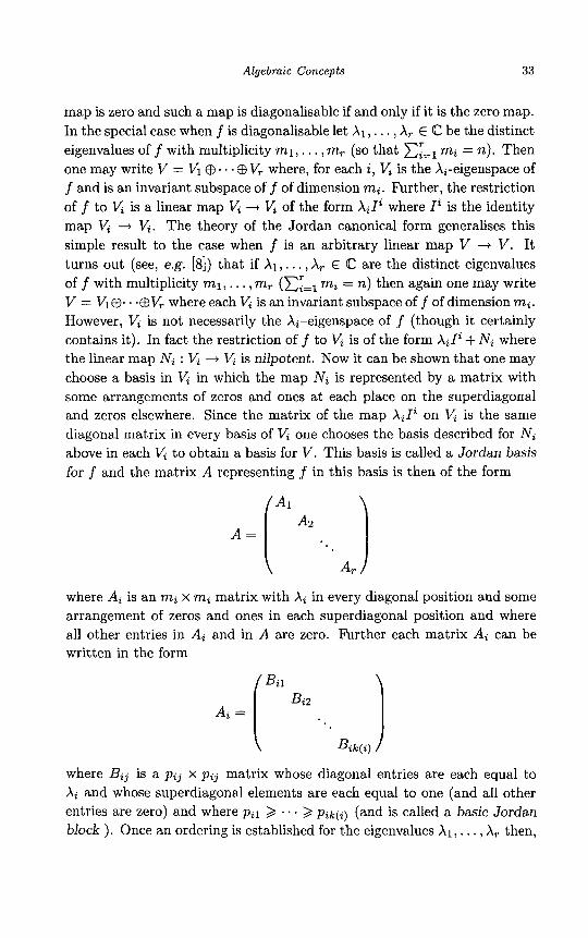
Algebraic Concepts 33
map is zero and such a map is diagonalisable if and only if it is the zero map. In the special case when f is diagonalisable let XI, . . . , A, E C be the distinct eigenvalues of f with multiplicity ml , . . . , m, (so that EL=, mi = n). Then one may write V = V1@. . . @ V, where, for each i, vi is the Xi-eigenspace of f and is an invariant subspace off of dimension mi. Further, the restriction of f to L$ is a linear map V, +. V, of the form A i l i where Ii is the identity map V, +. V,. The theory of the Jordan canonical form generalises this simple result to the case when f is an arbitrary linear map V +. V. It turns out (see, e.g. [8]) that if X1 , .. . , A, E C are the distinct eigenvalues of f with multiplicity ml , . . . , m, (C;=, mi = n) then again one may write V = V,@. . .@V, where each V, is an invariant subspace off of dimension mi. However, V, is not necessarily the Xi-eigenspace of f (though it certainly contains it). In fact the restriction of f to V, is of the form A i l i + Ni where the linear map Ni : V, --f V, is nilpotent. Now it can be shown that one may choose a basis in vi in which the map Ni is represented by a matrix with some arrangements of zeros and ones at each place on the superdiagonal and zeros elsewhere. Since the matrix of the map &Ii on V, is the same diagonal matrix in every basis of V, one chooses the basis described for Ni above in each V, to obtain a basis for V. This basis is called a Jordan basis for f and the matrix A representing f in this basis is then of the form
where Ai is an mi x mi matrix with Xi in every diagonal position and some arrangement of zeros and ones in each superdiagonal position and where all other entries in Ai and in A are zero. Further each matrix Ai can be written in the form
Ai =
Bik(i)
where Bij is a pij x pij matrix whose diagonal entries are each equal to Xi and whose superdiagonal elements are each equal to one (and all other entries are zero) and where pi1 2 . * 2 pik(i) (and is called a basic Jordan block ). Once an ordering is established for the eigenvalues XI , . . . , A, then,
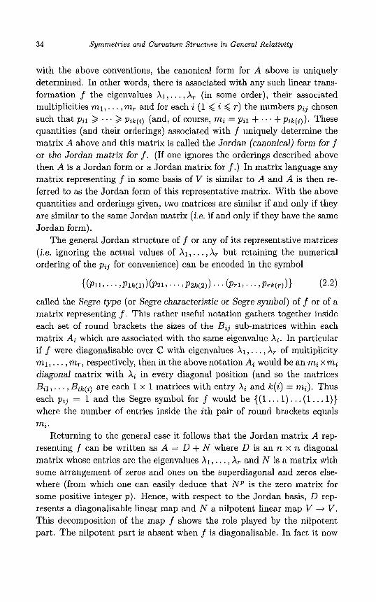
34 Symmetries and Curvature Structure in General Relativity
with the above conventions, the canonical form for A above is uniquely determined. In other words, there is associated with any such linear trans- formation f the eigenvalues XI,. . . , A, (in some order), their associated multiplicities ml , . . . , m, and for each i (1 < i 6 T ) the numbers pij chosen such that pi1 2 . . . 2 p i q i ) (and, of course, mi = pi1 + . . . + p q i ) ) . These quantities (and their orderings) associated with f uniquely determine the matrix A above and this matrix is called the Jordan (canonical) form for f or the Jordan matrix for f. (If one ignores the orderings described above then A is a Jordan form or a Jordan matrix for f.) In matrix language any matrix representing f in some basis of V is similar to A and A is then re- ferred to as the Jordan form of this representative matrix. With the above quantities and orderings given, two matrices are similar if and only if they are similar to the same Jordan matrix (i.e. if and only if they have the same Jordan form).
The general Jordan structure of f or any of its representative matrices (i.e. ignoring the actual values of X I , . . . , A, but retaining the numerical ordering of the pij for convenience) can be encoded in the symbol
((p111 ' ' ' , P l k ( l ) ) ( P 2 1 I ' ' ' , p 2 k ( 2 ) ) ' ' ' b - 1 1 ' ' ' l p T k ( T ) ) } (2.2)
called the Segre type (or Segre characteristic or Segre symbol) of f or of a matrix representing f. This rather useful notation gathers together inside each set of round brackets the sizes of the Bij sub-matrices within each matrix Ai which are associated with the same eigenvalue X i . In particular if f were diagonalisable over G with eigenvalues X 1 , . . . , X r of multiplicity ml , . . . , m,, respectively, then in the above notation Ai would be an mi x mi diagonal matrix with X i in every diagonal position (and so the matrices Bi l l , . . , B i k ( i ) are each 1 x 1 matrices with entry X i and k ( i ) = mi). Thus each p i j = 1 and the Segre symbol for f would be ((1.. .1). . . (1.. .1)} where the number of entries inside the ith pair of round brackets equals mi.
Returning to the general case it follows that the Jordan matrix A rep- resenting f can be written as A = D + N where D is an n x n diagonal matrix whose entries are the eigenvalues XI , . . . , A, and N is a matrix with some arrangement of zeros and ones on the superdiagonal and zeros else- where (from which one can easily deduce that NP is the zero matrix for some positive integer p). Hence, with respect to the Jordan basis, D rep- resents a diagonalisable linear map and N a nilpotent linear map V -+ V . This decomposition of the map f shows the role played by the nilpotent part. The nilpotent part is absent when f is diagonalisable. In fact it now
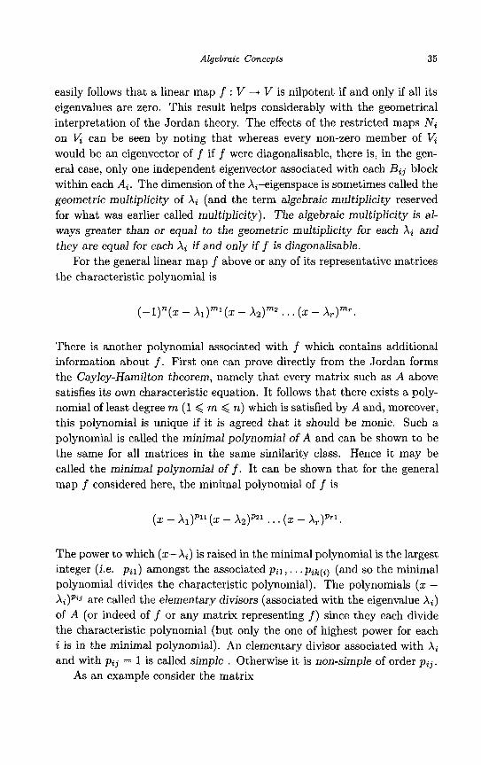
Algebraic Concepts 35
easily follows that a linear map f : V -+ V is nilpotent if and only if all its eigenvalues are zero. This result helps considerably with the geometrical interpretation of the Jordan theory. The effects of the restricted maps Ni on V, can be seen by noting that whereas every non-zero member of Vi would be an eigenvector of f if f were diagonalisable, there is, in the gen- eral case, only one independent eigenvector associated with each Bij block within each Ai. The dimension of the Xi-eigenspace is sometimes called the geometric multiplicity of Xi (and the term algebraic multiplicity reserved for what was earlier called multiplicity). The algebraic multiplicity is al- ways greater than or equal to the geometric multiplicity for each X i and they are equal for each X i if and only i f f is diagonalisable.
For the general linear map f above or any of its representative matrices the characteristic polynomial is
There is another polynomial associated with f which contains additional information about f . First one can prove directly from the Jordan forms the Cayley-Hamilton theorem, namely that every matrix such as A above satisfies its own characteristic equation. It follows that there exists a poly- nomial of least degree m (1 < m < n) which is satisfied by A and, moreover, this polynomial is unique if it is agreed that it should be monic. Such a polynomial is called the minimal polynomial of A and can be shown to be the same for all matrices in the same similarity class. Hence it may be called the minimal polynomial off. It can be shown that for the general map f considered here, the minimal polynomial of f is
The power to which (.-Xi) is raised in the minimal polynomial is the largest integer (i.e. pil) amongst the associated pi1 , . . . p i~ ( i ) (and so the minimal polynomial divides the characteristic polynomial). The polynomials (z - Ai)Pij are called the elementary divisors (associated with the eigenvalue Xi) of A (or indeed o f f or any matrix representing f) since they each divide the characteristic polynomial (but only the one of highest power for each i is in the minimal polynomial). An elementary divisor associated with X i
and with p i j = 1 is called simple . Otherwise it is non-simple of order pij. As an example consider the matrix

36 Symmetries and Curvature Structure in General Relativity
A =
y; 0 ‘TIC! ... .......
where a, p, y and 6 are distinct and all non-recorded entries are zero. In the above notation the Ai blocks are shown with unbroken lines whilst the Bij
blocks within them are indicated with broken lines. The eigenvalues and the algebraic multiplicities are a(6), p(2), y(2) and 6(1). The characteristic polynomial is (x - a)6 (x - /?)2 (x - ~ ) ~ ( x - 6) whilst the minimal polynomial is (x - - p)’(x - y)(x - 6). The Segre type is {(321)(2)(11)(1)} and the elementary divisors are (z - a)3, (x - a)2 , (x -a) , (x - p)2 , (x - y) and (x - 6). There are seven independent eigenvectors which may be chosen as having a one in the third (respectively the fifth, sixth, eighth, ninth, tenth and eleventh) slots, respectively, in C1’ and zero elsewhere, the eigenvalues being, respectively, a, a , a, p, y, y and 6. The geometric multiplicities of the eigenvalue a is thus 3, of p is 1, of y is 2 and of 6 is 1. In writing out Segre types it is convenient to omit the round brackets around a single digit. Thus the above Segre type would be {(321)2(11)1}.
The above discussion of the Jordan canonical form was applied to a vector space V over the algebraically closed field @. However, some of the applications of this theory are to the case of a vector space V over IR and, as discussed earlier, R is not algebraically closed. Nevertheless if f is a linear transformation from an n-dimensional real vector space V to itself and all the roots of the characteristic equation off lie in IR then the Jordan theory discussed here and all the attendant notation still applies. If, on the other hand, a complex conjugate (non-real) pair of solutions of the characteristic polynomial arise they lead to a 2-dimensional invariant subspace of f as described earlier and this remark will be sufficient for the purposes of this text. One could handle this situation by extending f to the complexification of V where the Jordan theory applies. In fact, if one regards this theory as a classification of matrices by similarity, the problem is not affected by such an extension. This follows because two real matrices
Algebraic Concepts 37
are similar over R if and only if they are similar over @. (In fact, more can be proved [12].)
A few closing remarks regarding the Jordan canonical form can now be made. Again let V be a vector space over F (= R or C ) of finite dimension n and let f be a linear map f : V ---f V . An eigenvalue X of f may be “degenerate” in two different ways; firstly due to the appearance of two elementary divisors of f (simple or non-simple) each associated with the same eigenvalue X off and secondly due to the appearance of a non-simple elementary divisor associated with A. The former can, in a sense, be r e garded as an “accidental” degeneracy (i.e. the accidental equality of the two elementary divisors) and is indicated by the use of round brackets in the Segre characteristic of f . The latter is indicated by a digit greater than one in the Segre characteristic. An eigenvalue can, of course, be degener- ate in both ways. The difference between these two types of degeneracy is reflected to some extent in the differences between the geometric and al- gebraic multiplicity of the eigenvalue. Here, an eigenvalue X will be called non-degenerate (respectively, degenerate) if the A-eigenspace has dimension 1 (respectively, > 1).
Using the notation of the preceding paragraph one might ask how tightly the Jordan basis for f is determined (assuming that, if F = R, all eigenvalues of f are real). If f may be represented by a diagonal matrix (in a Jordan basis of eigenvectors { e i } ) then any other Jordan basis {ei} for f is related to the original one by linear transformations of the basis members within the eigenspaces of f (and, in particular, ei = piel,.. . ,ek = p,e,, P I , . . . ,pn E F if the eigenvalues of f are distinct.) Other types of ambiguities in the Jordan basis are introduced (by the non-simple elementary divisors) if f is not diagonalisable. Now let A E M,(F) ( F = R or C). It is a well-known result that A is similar to its transpose. This result will be useful in a later chapter. It also shows that if (as some authors do) one takes the Jordan canonical matrices as being the transposes of the ones defined here, then nothing is changed. It is remarked here, for later reference, that if two matrices in M,F have the same characteristic and minimal polynomials they are not necessarily similar. This follows, for example, by considering two matrices of Segre types {(32)1} and { (311)1}, respectively, which each have characteristic polynomial (x - - p) and minimal polynomial (x - c ~ ) ~ ( x - p) for a , P E F .
Let V be a real vector space and f : V 4 V a linear map with a non-real conjugate pair of eigenvalues. Suppose that, when the situation
38 Symmetries and Curvature Strzlcture in General Relativity
is “complexified” (as described earlier) f is diagonalisable. Then one often says that “f is diagonalisable over C but not over IW” to describe this situation and the pair of symbols z z will be inserted in the Segre symbol for f. Thus if dimV = 4 and f has, say, two distinct real eigenvalues and a non-real conjugate pair of eigenvalues its Segre symbol will be written ( ~ ~ 1 1 ) (or { l lzz}) .
2.7 Lie Algebras
Let V be a vector space over a field F (= R or C). Then V is called an algebra if there is a binary operation on V , (u, v) 3 uv (u, v E V ) such that for a E F and u, v, w E V
(Al) (U + V)W = uw + vw (A2) U(V + W) = uv + uw (A3) a(uv) = (au)v = u(av)
[An algebra V satisfying the extra condition ( u v ) ~ = ~ ( v w ) is called associative.] If further V is a real vector space and satisfies, in addition to (Al) , (A2) and (A3) the conditions
(A4) (UV) = -(vu) (A5) U(VW) + V(WU) + W(UV) = 0
then V is called a Lie algebra. If V is a finite-dimensional Lie algebra of dimension n and {ei} is a basis for V then there exist real numbers c , b
such that eaeb = c:=l Cacbec. The numbers c , b are called the structure constants for V in the basis (e,) and, from (A4) and (AS) satisfy
The LLassociativel’ condition is not necessarily satisfied. The condition (A5) is sometimes referred to as the Jacobi identity. A subspace U of V which is itself a Lie algebra under the binary operation induced on it by V is called a (Lie) subalgebra of V. If V , W are Lie algebras and f : V + W is a vector space homomorphism (respectively, isomorphism) such that (with an obvious simplifying of notation) f(uv) = f(u)f(v) (u,v E V) then f is called a Lie algebra homomorphism (respectively, isomorphism), and V and W are said to be Lie algebra homomorphic (respectively, isomorphic).
Algebraic Concepts 39
The set M,R is a finite dimensional real vector space which becomes a Lie algebra if one defines the binary operation (A , B ) --t AB - BA.

This page intentionally left blank
Chapter 3
Topology
3.1 Introduction
Topology is one of the most important branches of mathematics. A topology for a set is a certain type of “structure” for that set which allows one to discuss sensibly such important concepts as ‘‘convergence” and “limits” of sequences in this set and the idea of a ‘kontinuous function” between such sets. It also permits the description of certain subsets of a set as “large” or %mall” and of points which are arbitrarily close to certain subsets of the set. Most geometrical “pictures” of mathematical constructions assume some topology on the set in question and hence its importance.
Perhaps a more natural “structure” for a set is a “distance structure” namely the ability to attach some positive real number to each pair of distinct points of the set (subject to certain sensible requirements) and which is interpreted as the “distance” between them. Such a “metric” structure should make sense of those important concepts described above which follow from a topological structure and hence should give rise to a natural topological structure for the set in question. However, the converse is not true in the sense that a definition of a topological structure has evolved during the 20th century which is sufficiently strong to do all that is required of it but which does not imply the existence of a “compatible” metric structure for the set concerned. Thus a topological structure is more general then a metric structure and the latter is a special case of the former. It follows that one can proceed either by starting with the axioms for a topological structure and show how a metric structure is a special case or by starting with the ideas of a metric structure and generalising to those of a topology. The former approach has much aesthetic appeal but its generality in the initial stages tends to obscure the proceedings. The second
41
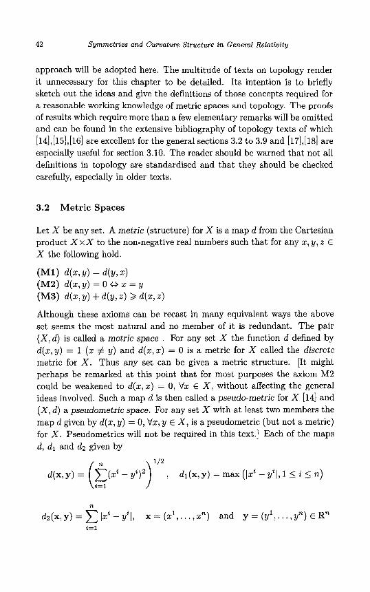
42 Symmetries and Curvature Structure in General Relativity
approach will be adopted here. The multitude of texts on topology render it unnecessary for this chapter to be detailed. Its intention is to briefly sketch out the ideas and give the definitions of those concepts required for a reasonable working knowledge of metric spaces and topology. The proofs of results which require more than a few elementary remarks will be omitted and can be found in the extensive bibliography of topology texts of which [14],[15],[16] are excellent for the general sections 3.2 to 3.9 and [17],[18] are especially useful for section 3.10. The reader should be warned that not all definitions in topology are standardised and that they should be checked carefully, especially in older texts.
3.2 Metric Spaces
Let X be any set. A metric (structure) for X is a map d from the Cartesian product X XX to the non-negative real numbers such that for any x, y, z E X the following hold.
(MI) 4 a : , Y ) = d ( y , z )
(M3) 4x7 Y) + d(y, 2) 3 d(z, z )
(M2) d ( x , y) = 0 H z = y
Although these axioms can be recast in many equivalent ways the above set seems the most natural and no member of it is redundant. The pair ( X , d ) is called a metric space . For any set X the function d defined by d ( z , y ) = 1 (x # y) and d ( x , z ) = 0 is a metric for X called the discrete metric for X. Thus any set can be given a metric structure. [It might perhaps be remarked at this point that for most purposes the axiom M2 could be weakened to d ( z , z ) = 0, Va: E X, without affecting the general ideas involved. Such a map d is then called a pseudo-metric for X [14] and ( X , d ) a pseudometric space. For any set X with at least two members the map d given by d ( z , y) = 0, Vx, y E X, is a pseudometric (but not a metric) for X. Pseudometrics will not be required in this text.] Each of the maps d, dl and dz given by
1 d l ( X , Y ) = max ( I xi - y i l , l 5 i 5 n)
n
d z ( x , y ) = lxi - yzl, x = (d,. . . ,P) and y = (y', . . . , yn) E Rn i=l
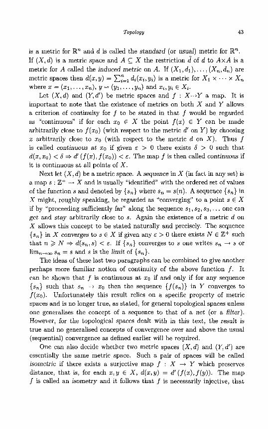
Topology 43
is a metric for Rn and d is called the standard (or usual) metric for JR”. If (X, d) is a metric space and A C X the restriction 2 of d to A x A is a metric for A called the induced metric on A. If (XI,&), . . . , (X,, d,) are metric spaces then d(z, y) = Cy=l &(xi, yi) is a metric for X1 x . . . x X , where z = (XI,. . . , z,), y = (yl , . . . , y,) and zi,yi E Xi .
Let (X,d) and (Y,d’) be metric spaces and f : X-+Y a map. It is important to note that the existence of metrics on both X and Y allows a criterion of continuity for f to be stated in that f would be regarded as “continuous” if for each 20 E X the point f(z) E Y can be made arbitrarily close to f (zo) (with respect to the metric d’ on Y ) by choosing z arbitrarily close to zo (with respect to the metric d on X ) . Thus f is called continuous a t 20 if given E > 0 there exists 6 > 0 such that d(z , zo ) < 6 + d’ (f (z), f (20)) < E . The map f is then called continuous if it is continuous at all points of X .
Next let (X, d) be a metric space. A sequence in X (in fact in any set) is a map s : Z+ -+ X and is usually “identified” with the ordered set of values of the function s and denoted by {s,} where s, = s(n). A sequence {s,} in X might, roughly speaking, be regarded as ‘‘converging’’ to a point s E X if by “proceeding sufficiently far” along the sequence s1, s2, sg, . . . one can get and stay arbitrarily close to s. Again the existence of a metric d on X allows this concept to be stated naturally and precisely. The sequence { s,} in X converges to s E X if given any E > 0 there exists N E Z+ such that n 2 N + d(s,,s) < E. If {s,} converges to s one writes s, 4 s or limn--tca s, = s and s is the limit of {s,}.
The ideas of these last two paragraphs can be combined to give another perhaps more familiar notion of continuity of the above function f . It can be shown that f is continuous at zo if and only if for any sequence {s,} such that s, --f zo then the sequence { f ( s , ) } in Y converges to f ( z0 ) . Unfortunately this result relies on a specific property of metric spaces and is no longer true, as stated, for general topological spaces unless one generalises the concept of a sequence to that of a net (or a filter). However, for the topological spaces dealt with in this text, the result is true and no generalised concepts of convergence over and above the usual (sequential) convergence as defined earlier will be required.
One can also decide whether two metric spaces (X,d) and (Y,d’) are essentially the same metric space. Such a pair of spaces will be called isometric if there exists a surjective map f : X Y which preserves distance, that is, for each z, y E X , d(z, y) = d’ (f(z),f(y)). The map f is called an isometry and it follows that f is necessarily injective, that
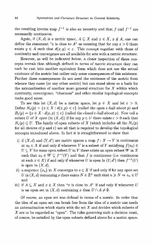
44 Symmetries and Curvature Structure in General Relativity
the resulting inverse map f-’ is also an isometry and that f and f - l are necessarily continuous.
Again, if ( X , d ) is a metric space, A & X and x E X , x !j! A, one can define the statement “x is close to A’ as meaning that for any E > 0 there exists y E A such that d ( z , y ) < E . This concept together with those of continuity and convergence are all available for sets with a metric structure.
However, as will be indicated below, a closer inspection of these con- cepts reveals that although defined in terms of metric structure they can each be cast into another equivalent form which does not use the actual existence of the metric but rather only some consequences of this existence. Further these consequences do not need the existence of the metric from whence they came (or any other metric) but can stand alone as a basis for the axiomatisation of another more general structure for X within which continuity, convergence, “closeness” and other similar topological concepts make good sense.
To see this let ( X , d ) be a metric space, let p E X and let E > 0. Define N E ( p ) = {x E X : d ( z , p ) < E } (called the open &-ball about p ) and B,(p) = {x E X : d ( x , p ) 5 E } (called the closed &-ball about p ) . Now call a subset U of X open (in ( X , d ) ) if for any p E U there exists E > 0 such that N,(p) C U . The family of open subsets of X (which includes all the N E ( p ) for all choices of p and E ) are all that is required to develop the topological concepts introduced above. In fact it is straightforward to show that
i) if ( X , d ) and (Y ,d ’ ) are metric spaces a map f : X + Y is continuous at zo E X if and only if whenever V is a subset of Y satisfying f ( x 0 ) E U C V for some open subset U in Y there exists an open subset W in X such that xo E W C f - l (V) and that f is continuous ( i e . continuous at each x E X ) if and only if whenever U is open in (Y, d’) then f - ’ (U) is open in ( X , d) ,
ii) a sequence { s,} in X converges to s E X if and only if for any open set U in ( X , d ) containing s there exists N E Z+ such that n 2 N + s, E U and
iii) if A & X and x E X then “x is close to A” if and only if whenever U is an open set in ( X , d ) containing x then U n A # 0.
Of course, an open set was defined in terms of a metric. In order that the idea of an open set can break free from the idea of a metric one needs an axiomatisation which starts with the set X and decides which subsets of X are to be regarded as “open”. The rules governing such a decision must, of course, be satisfied by the open subsets defined above for a metric space.
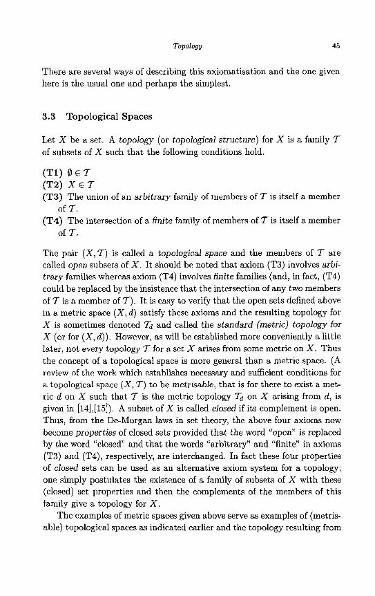
Topology 45
There are several ways of describing this axiomatisation and the one given here is the usual one and perhaps the simplest.
3.3 Topological Spaces
Let X be a set. A topology (or topological structure) for X is a family 7 of subsets of X such that the following conditions hold.
(Tl) 0 ~ 7 (T2) X E 7 (T3) The union of an arbitrary family of members of 7 is itself a member
of 7. (T4) The intersection of a finite family of members of 7 is itself a member
of 7 .
The pair ( X , 7 ) is called a topological space and the members of 7 are called open subsets of X . It should be noted that axiom (T3) involves arbi- trary families whereas axiom (T4) involves finite families (and, in fact, (T4) could be replaced by the insistence that the intersection of any two members of 7 is a member of 7) . It is easy to verify that the open sets defined above in a metric space (X, d ) satisfy these axioms and the resulting topology for X is sometimes denoted and called the standard (metric) topology for X (or for (X, d) ) . However, as will be established more conveniently a little later, not every topology 7 for a set X arises from some metric on X . Thus the concept of a topological space is more general than a metric space. (A review of the work which establishes necessary and sufficient conditions for a topological space ( X , 7) to be metrisable, that is for there to exist a met- ric d on X such that 7 is the metric topology ’& on X arising from d, is given in [14],[15]). A subset of X is called closed if its complement is open. Thus, from the De-Morgan laws in set theory, the above four axioms now become properties of closed sets provided that the word “open” is replaced by the word LLclosed and that the words “arbitrary” and “finite” in axioms (T3) and (T4), respectively, are interchanged. In fact these four properties of closed sets can be used as an alternative axiom system for a topology; one simply postulates the existence of a family of subsets of X with these (closed) set properties and then the complements of the members of this family give a topology for X.
The examples of metric spaces given above serve as examples of (metris- able) topological spaces as indicated earlier and the topology resulting from

46 Symmetries and Curvature Structure in General Relativity
the standard metric on R” is called the standard (or usual) topology on R”. In fact R” will always be assumed to have this topology unless otherwise stated. Some other less standard examples can now be given. Let X be any set. If 7 is the family of all subsets of X then 7 is a topology for X called the discrete topology (and is the metric topology for X with the discrete metric). Alternatively one could take 7 = (0, X} as a topology for X (the indiscrete topology for X). In this case 7 is not metrisable if X contains at least two members. Another topology for X is the family of subsets of X whose complement is finite, together with the set 0. This topology, called the co-finite topology for X , is just the discrete topology for X if X is finite. If in the last two sentences finite is replaced by countable then one obtains the co-countable topology for X. Again, one could start with a pseudometric space and construct a topology for it from the pseudometric just as was done above for a metric space. For a metric space, any closed ball is easily shown to be a closed set in the resulting topology and thus open and closed intervals in IR are open and closed sets respectively in the (standard) topology resulting from the standard metric on R.
Let (X,T) be a topological space and let x E X . A subset N of X containing x is called a neighbourhood of x if there exists an open set U such that x E U 5 N . A neighbourhood N of x need not be open nor need it be a neighbourhood of some point y E N , y # x. A subset N of X is a neighbourhood of each of its points if and only if N is open in X . Again let x E X and A C: X. Then x is a limit point of A if every open set containing z intersects A in some point other than (possibly) z. (For x $ A this is the idea of “closeness” mentioned earlier.) This definition has the intuitively pleasing consequence that a subset A X is closed if and only if A contains all its limit points. These concepts lead to two operations applicable to any subset A of X which, respectively, reduce it to its “largest contained” open subset and increase it to its “smallest containing” closed subset. For the first one define the interior of A , int A , to be the set of all points in A of which A is a neighbourhood and for the second one define the closure A of A to be the union of A and all its limit points. It is then straightforward to show that int A is open, that A is closed, and that if U is an open set and B a closed set such that U C A C: B then U & intA A C A C B. It follows for any subset A that A is open if and only if A = int A, that A is closed if and only if A = A and that X \ A = X \ int A. A closely related concept is that of boundary. A point x E X is called a boundary point of A C X if x $ int A and x @ int(X \ A). The boundary S(A) of A is the set of all boundary points of A. Thus S(A) = A n (X \ A ) (and
Topology 47
is hence always a closed set) and 6 ( A ) = 6(X \ A ) . An intuitively pleasing result regarding the boundaries of open and closed sets is the pair of facts that A is closed if and only if 6(A) C A and A is open if only only if A n &(A) = 0. For any topological space (XI 7) and subset A , X admits a disjoint decomposition X = int A U b(A) U int(X \ A ) . A subset A of X is called dense (in X ) if A = X and a subset B of X is called nowhere dense if int B = 0. These definitions allow a statement of “topological” size. One can think of a subset A of X as being LLlargell in (the topology of) X if it is open and dense and a subset B of X as being “small” in (the topology of) X if it is closed and nowhere dense. Also a subset A of X is dense if and only if int(X \ A ) = 0 and so the complement of an open, dense subset is closed and nowhere dense, and vice versa. It should be understood here that a subset A of X which is merely dense need not be “large” if it is not open; it may simply be “well distributed” as the subset Q of R shows since, in the usual topology on R, Q is dense but not open. It is easily checked that the intersection of finitely many open dense subsets of a topological space is open and dense and hence that the union of finitely many closed, nowhere dense sets is closed and nowhere dense.
The concepts of continuity and convergence described earlier in a met- ric space are conveniently described in any topological space (X,7) . A sequence {x,} in X is said to converge with limit x if given any neighbour- hood A of x there exists N E Z+ such that n 2 N * x, E A. Also, if (X, 7) and (Y, 7’) are topological spaces and f : X -+ Y a map then f is called continuous at x E X if f - l ( N ) is a neighbourhood of x whenever N is a neighbourhood of f(x). Then f is called continuous if it is continuous at each x E X . It follows that f is continuous if and only if whenever U is open in Y , f-l(U) is open in X (and that f is continuous if and only if whenever V is closed in Y , f-’(V) is closed in X) . Further, if (X,‘T), (Y, 7’) and ( Z , 7 ” ) are topological spaces and f : X -+ Y and g : Y t 2 are continuous then g o f : X -+ Z is continuous. If (X, 7) and (Y, 7’) are topological spaces and f : X -+ Y is a bijective map such that f and f-’ are continuous then f is called a homeomorphism and (X,‘T) and (Y,‘T’) are said to be homeomorphic (ie. topologically identical). The continuity of both f and f-’ is essential here since one of these maps could be contin- uous and the other not (as for example occurs if X = Y with X containing more than one member, if f is the identity map on X and if 7 and 7’ are the discrete and the indiscrete topologies for XI respectively). Clearly, the relation of being homeomorphic is an equivalence relation on topological spaces.
48 Symmetries and Curvature Structure in General Relativity
The above paragraphs give the definition and basic properties of topo- logical spaces. They apply to metric spaces through the natural topology on such spaces induced by the metric. The topology of a metric space does not require all the detail of the metric but only the open sets that it leads to. For example, the three metrics on R” described in the previous section are different metrics for R” but it is easy to show that each gives rise to the same topology for R” (i.e. the standard topology). The topology is thus blind to the differences between these metrics. One calls two metrics d and d’ for the same set X equivalent if the resulting metric topologies 7 d and Gt are equal. If such is the case, whilst d and d’ can be different metrics for X (i.e. the identity map ix : X -+ X is not an isometry), the topological spaces ( X , 7 d ) and ( X , I d , ) are identical (i.e. ix is a homeomorphism be- tween them). Of course there may still exist an isometry f between ( X , d ) and (X ,d ’ ) with f # ix but there need not. For let X = R and d be the usual metric for R. The map f : z -+ tan z is a bijection (- %,$) -+ R and gives rise to a metric d’ on R by “transferring” the metric d (restricted to (-;, ;)) onto R, i.e. d’(z, y) = d (f-’(z), f - l (y ) ) . It clearly follows that there is no isometry between (R,d) and (R,d’) but ( R , G ) and (R,Idt)
are homeomorphic (and the identity map i~ is such a homeomorphism). One is thus led to the concept of a metric property of a metric space (one which if true for ( X , d ) is true for all metric spaces isometric to ( X , d ) ) and a topological property of ( X , d ) (one which if true for ( X , d) is true for any metric space homeomorphic to ( X , d) ) . Thus topological properties are metric properties but not necessarily vice versa. A metric property (but not a topological property) may be destroyed by changing the metric d for a certain set X to a metric d‘ equivalent to d. A rather nice example of this feature is the concept of a bounded metric space. A metric space ( X , d ) is called bounded (and d is called a bounded metric for X ) if there exists Q E R such that d ( a , y ) < Q for each z,y E X . A subset A of a metric space ( X , d ) is called bounded if A with its induced metric is a bounded metric space. Now for any metric space ( X , d ) the function d’ defined by d’(z, y) = min (d (z , g ) , 1) can be shown to be a bounded metric for X which is equivalent to d. Hence any metric space is homeomorphic to (but not necessarily isometric to) a bounded metric space. Hence “boundedness” is a metric property but not a topological property of metric spaces.

Topology 49
3.4 Bases
If (XI d ) is a metric space and U is an open subset of X then for each x E U there exists 6 > 0 such that z E Nb(z) U . It follows that U is the union of open sets of the form NE(x) where z ranges over all the points of U and the positive real number E = E ( X ) is determined by x. Thus the open balls in X constitute a privileged subfamily of 7 d from which all open subsets of X can be constructed. This particularly useful construction can be applied to a general topological space (X, 7). A subfamily B of 7 is called a base (or basis) for 7 if each member U of 7 is a union of members of B. Then 7 is said to be generated by B. It follows that €3 is a base for 7 if and only if for each x E X and each open set U of X containing x there exists B E 23 with x E B & U . For any topological space ( X , T ) , 7 is itself a (rather uninteresting) base for 7 whilst the family of (finite) open intervals is a base for R with its usual topology. A more interesting base for this last topological space is the (countable) family of (finite) open intervals with rational endpoints. As described above, the family of all open balls in a metric space (XI d ) is a base for 7 d .
The idea of a base can be “reversed” by taking a set X and a family B of subsets of X and asking if there exists a topology 7 for X for which B is a base. By using the definition of a base above it is not hard to prove that such a topology exists if and only if X equals the union of all members of B and if whenever B1, B2 E B and p E B1 n B2 there exists B E B such that p E B c B1 n Ba. It is clear from the examples given above that a particular topological space may possess many bases. An easily proved criterion restricting this situation says that if X is a set and B and B’ are families of subsets of X which are bases for the topologies 7 and 7’ on X then 7 = 7’ if and only if (i) for each B E B and each x E B there exists B’ E B‘ with x E B’ c B and (ii) for each B’ E B’ and each z E B’ there exists B E B with x E B & B’. If 7 = 7’ the bases B and B‘ are said to be equivalent.
If X is a set and B a family of subsets of X one sometimes requires a topology 7 for X in which the members of B are open sets (i.e. B c 7). Of course if B satisfies the conditions for being a base for some topology on X then one could identify this topology with 7. In any case one could solve the problem trivially by giving X the discrete topology. However, given that the union of the members of B equals XI there is a more interesting and usually more useful solution to the problem which, in a precise sense, contains no more sets than is necessary. One simply notes that the family
50 Symmetries and Curvature Structure an General Relativity
B’ consisting of all finite intersections of members of B is a base for some topology 7 on X and that if 7’ is any other topology for X for which all members of B are open, I C 7‘. If this is the case B is called a subbase (or subbasis) for the topology 7 and is said to generate I. For example, the family of subsets of R which are either of the form (--00, a ) or ( a , m) for each a E R is a subbase for the usual topology on R.
It is often important to know those open subsets of a topological space (X, 7) which contain a particular point x E X. A family V of open subsets each of which contains x is called a local base (or basis) at x if whenever U E 7 and x E U there exists D E V such that x E D c U . The connection between a base for (X, I) and the collection of local bases at each x E X is easily established. In fact if B is a collection of subsets of X then 13 is a base for (X,I) if and only if for each x E X the family B, = { B E B : x E B } is a local base at x.
Two rather important definitions for a topological space can now be given. A topological space is called first countable if there is a local base at each x E X with countably many members (i.e. a countable local base) and it is called second countable if it admits a base with countably many members (a countable base). Clearly, by the result at the end of the last paragraph a second countable topological space is necessarily first count- able but the converse result is false as is easily seen by considering an un- countable set X with discrete topology. First countable topological spaces are important in the theory of convergence. In fact there is a sense in which “sequences are adequate” for describing matters of convergence in first countable topological spaces whereas for non-first countable spaces the more general concept of convergence involving nets and filters must be used. A detailed discussion of this can be found in [14]-[16]. Only first countable topological spaces will be required in this text (and it should be pointed out in this context that any metric space is first countable in its metric topology since the family N L ( x ) (n E Z+) is a countable local base at any x E X, but not necessariiy second countable). The concept of second countability is important in that it leads to several other useful topological properties. One rather interesting one is that a second count- able topological space ( X , 7 ) is “not too large” in the sense that if A c X and A is uncountable then A is “cramped” at some point or, more precisely, some point of A is a limit point of A. A metric space need not be second countable but, as shown earlier, the set R with its usual topology admits a countable base and is thus second (and hence first) countable.
Bases, local bases and subbases can be rather useful. For example, a
Topology 51
map f : X .+ Y between topological spaces is continuous if and only if the inverse image under f of each member of a base (or, in fact, each member of a subbase) of Y is open in X . Also, a sequence {x,} in a topological space X converges to 20 E X if and only if for any member B of a local base at xo there exists N E Zf such that n 2 N + x, E B.
3.5 Subspace Topology
Let ( X , d ) be a metric space, A a subset of X and d the induced metric on A. The open &-balls in ( A , J ) are merely the intersections with A of the sets NE(x) for each x E A and the open subsets of A (in the metric topology on A arising from the metric d ) are then the intersections with A of open subsets in X . Thus one sees how a natural topology might be induced on any subset A of any topological space ( X , 7 ) . One defines a topology 7 on A by setting 7 = {U’ L A : U‘ = A n U , U E I}, that is, the open subsets of ( A , 7 ) are precisely the intersections with A of open subsets of X . That T is a topology for A is easily established and is called the subspace or relative topology on A (from the topology 7 on X ) . One is then relieved to find that if A and B are subsets of X with B A then the subspace topology on B due to its being a subset of X (with the topology 7) is the same as its subspace topology as a subset of A when the latter has its subspace topology 7 from (X, 7). This is easily done and the topological space (A , 7 ) is called a (topological) subspace of ( X , 7). Subspace topologies are well-behaved. It is easy to check, for example, that the closed subsets in ( A , 7 ) are precisely the intersections with A of the closed subsets of X and that if C is a subset of A then a point p E A is a limit point of C in the topology on A if and only if it is a limit point of C in the original topology 7 on X. Closures and interiors in subspace topologies can also be easily handled and if N C A is a neighbourhood of x E A in 7 then N n A is a neighbourhood of x in 7’. Also, if B is a base for X then the intersection of the members of B with A give a base for the topology T on A. A similar result holds for local bases. Now suppose ( X , 7) and (Y, 7’) are topological spaces, A L X and f : X -+ Y a continuous map. Then the restriction f l ~ : A -+ Y is continuous as a map between the topological spaces (A ,T) and (Y,7’) . A similar result holds for continuity at individual points of A. Further, the continuity of f : X -+ Y is equivalent to the continuity of the map f : X -+ f (X) defined by f(~) = f(z) when f ( X ) has subspace topology from (Y ,7 ’ ) .
52 Symmetries and Curvature Structure in General Relativity
It also follows that the inclusion map i~ : A + X is continuous when A has subspace topology. In fact 7’ is the “smallest” topology for A (in an obvious sense) which would make ZA continuous and this result is often invoked to give an alternative definition of subspace topology. Finally, if {z,} is a sequence in A and z o E A then z, -+ zo in the topological space (X, 7) if and only if z, -+ z o in the topological space (A , 7).
If ( X , d ) is a metric space and A C X the topology 7 2 on A arising from the naturally induced metric 2 on A is the same as the subspace topology on A arising from the topology 7 d on X. It is interesting to ask which topological properties of the topological space (X, 7) are inherited by its subspaces. Such properties are termed hereditary and the topological properties of being first or second countable and of being metrisable are, from the above discussion, each hereditary. Others will be encountered later.
A subset A of a topological space X is called discrete (in X ) or a set of isolated points if given a E A there is an open subset U of X satisfying a E U and U n A = { u } . In other words, the induced topology on A from 7 is discrete.
3.6 Quotient Spaces
Let (X, 7) be a topological space and let N be an equivalence relation on X which gives rise to a partition P of X (so that a member of P containing z E X consists of all points y of X such that z - y). Let p be the map X 4 P which associates with each z E X the unique member of P in which it lies. The family {U C P : p - l ( U ) E 7 ) is a topology for P called the quotient topology for P and the resulting topological space is called the quotient space of X by - and will be denoted by X/ N. The map p (called the projection map) is now continuous. Sometimes (and for fairly obvious reasons) the quotient topology is called the identification topology since one can regard those members of X which lie inside a single member of P as having been (topologically) “identified”. Thus one obtains P from X by “identification” from the relation N. As an example let ( X , 7) be the subset [0,1] of R with subspace topology from the usual topology on R and let P consist of the subsets {z} for each z E (0 , l ) and the subset {0,1}. Then the resulting quotient space as described above is homeomorphic to the subset S’ E { (z, y) : x2 + y2 = 1) of R2 with subspace topology from the usual topology on R2.
Topology 53
3.7 Product Spaces
It was shown in section 3.2 that if (XI, dl), . . . , (X,, d,) were metric spaces then a metric could be constructed on the set X = X 1 x . . . x X,. However, the metric given is one of several metrics for this product competing for the title of “natural” (cfthe metrics for Rn given earlier). Fortunately, they are equivalent metrics for this product and the (unique) topology they generate on X has the property that each open set is a union of open sets of the form U1 x . . . x U, where Ui is open in ( X i , di). This leads to the idea of the (topological) product of topological spaces ( X I , ‘&) , . . . , (X,, 7,). Consider the family of subsets of the product set X of the form U1 x . . . x U, where Ui E x. This family is readily shown to be a base for a topology 7 on X . The topology 7 is called the product topology for X and (X,‘T) is called the (topological) product (space) of (XI, ‘&), . . . , (X,, 7,). The projection maps pi : X -+ Xi defined by pi(x1 , .. . , 2,) = xi are then continuous and, in fact, the product topology on X is the smallest topology (in an obvious sense) for which the maps p i are continuous. The product topology on X can also be regarded as being generated by the subbase of subsets of the f o r m p i l ( U ) = X 1 x . . . x X i - l x U x X i + l x . . . x X , f o r e a c h U ~ X a n d each i, 1 6 i 6 n. The finite intersections of these subbase members yield the base for 7 given above. If {zm} is a sequence in X then zm -+ xo E X if and only if pi(x,) 4 p i ( z 0 ) in ( X i , x) for each i. If Ai C X i (1 < i < n) are subspaces of Xi the product topology on A1 x . . . x A, equals its subspace topology from X I x . . . x X,. The standard topology on Rn is the product topology on R x . . . x R (n times) when R has its standard topology. It is often useful to note that a map from a topological space Y into the above product space X is continuous if and only if p i 0 f : Y 4 X i is continuous for each i. Here only a finite product of topological spaces has been considered. Infinite products can be handled but extra difficulties are encountered. They will not be required in this text and are not discussed here. Further details are available in [14]-[16].
3.8 Compactness and Paracompactness
Suppose one considers R” with its usual metric and topological structure and asks if one can attach any meaning to the concept of a ‘Lsmallll subset A of R”. A concept of “smallness” (i.e. the closed and nowhere dense concept) was discussed earlier in this chapter. Another such idea can now
54 Symmetries and Curvature Structure in General Relativity
be introduced. Merely asking that A be a bounded subset is inadequate since such a subset with its subspace topology might be homeomorphic to R” itself (e.g. the subset (0 , l ) of R). More is clearly required. The classical concept of “small” was that A should be a closed and bounded subset of R”. However this definition contains reference to the metric on R” and may not be a topological property. Fortunately this definition is, for R”, equivalent to the topological statement that if B is a family of open subsets of Rn whose union contains A then the union of some finite subfamily of B will also contain A. The satisfying of this definition by A would thus be unaffected by a change of metric to another equivalent metric. Further this equivalent condition can now be taken over to any topological space and leads to the important idea of compactness. It was, the author believes, Hermann Weyl who described this concept rather beautifully by defining a compact city as one which could be patrolled by a finite number of arbitrarily short-sighted policemen!
Let ( X , I ) be a topological space and let B be a family of subsets of X. If the union of the members of B equals X, B is called a covering of X (or one says that B covers X) and if each member of B is open it is an open covering of X. If a subfamily B’ of B also covers X, B’ is called a subcovering of B. The topological space (X, I) is called compact if each open covering of X contains a finite subcovering. A subspace of X is called compact if it is compact in its subspace topology. It is easy to see that W” is not compact for any n E Z+ and less easy to see that the subspace [a,b] of R (a ,b E R, a < b) is a compact subspace of Iw as is the sphere S”-l = {x E R” : 1x1 = 1) as a subspace of Wn. [Earlier in this chapter it was suggested that second countable topological spaces were in some sense not too “large” because any uncountable subset of such a space necessarily contained a limit point of itself. In fact any second countable space, whilst not in general compact, has the property that any open covering of it contains a countable subcovering.] It can be shown that a subspace of a compact topological space need not itself be compact but that a closed subspace of a compact space is compact.
There are some rather important results regarding continuous functions on compact topological spaces. Firstly, if X and Y are topological spaces with X compact and if f : X 4 Y is continuous then f ( X ) is a compact subspace of Y (and hence Y is necessarily compact if f is surjective). It follows that any quotient space of a compact space is compact. Secondly, if X is a compact space and R has its usual topology and if f : X -+ W is a continuous real valued function on X then f is bounded and attains its

Topology 55
bounds (that is f (X) is a bounded subset of R and there exist x ,y E X such that f (x) = sup[f(X)] and f (y ) = inf[f(X)]). It follows that if, in addition, f is a positive function (i.e. f (x ) > 0 for each s E X) then f is “bounded away from zero” (i.e. there exists E E R, E > 0, such that f ( s ) 2 E
for each x E X). Finally, let (X, I) be the topological product of the spaces (XI, Z), . . . , (Xn, 7n). If X is compact then it follows from the above and the continuity and surjectivity of the projection maps pi : X + Xi that each of the spaces Xi is compact. The converse of this result is also true, that is, the compactness of each of the Xi implies the compactness of X. This result stated here for finite products can be extended to infinite products and is the theorem of Tychonoff [14], [15].
A topological space can be quite pathological if it is restricted by nothing more than the axioms of a topological space. This generality is, on the one hand, the reason for their wide applicability but, on the other hand, often restricts progress in particular areas of investigation. Thus these axioms are occasionally supplemented by extra restrictions often inspired by the “standard topological spaces. Extra axioms governing the “topological separation” of points are, in particular, often imposed. These are the so- called separation axioms and only three of these will be discussed here. A topological space X is called a TI space if given s, y E X, x # y, there exist open subsets U and V such that x E U , y # U , y E V, x # V. This is equivalent to the statement that all subsets of X containing a single point of X are closed. A topological space X is called a T2 space (or more commonly a Hausdorff space) if given s , y E X, s # y, there exist open subsets U and V such that x E U , y E V and U n V = 8. Finally, a topological space X is called normal if for each disjoint pair of closed subsets A and B of X there exist disjoint open subsets U , V such that A C U , B C V. Every subspace of a Hausdorff space is Hausdorff and every closed subspace of a normal space is normal. The extra “separation” provided in a Hausdorff space removes many pathologies. Clearly every Hausdorff space is a TI space and every metric space is Hausdorff and (less obviously) normal. Recalling the discussion above about the definition of compactness it is reassuring to note that any compact subspace of a Hausdorff space is closed. It can now be checked that a continuous bijective map from a compact to a Hausdorff topological space is a homeomorphism. It was stated above that every continuous real valued function on a compact topological space is bounded. For a metric space the converse is true, that is, if every real valued continuous function on a metric space is bounded then it is compact. It is perhaps also relevant to remark that although the
56 Symmetries and Curvature Structure in General Relativity
definition of compactness used here is now standard in topology there have been several other (non-equivalent) competing definitions.
A covering I3 of a topological space X is called locally finite if each x E X is contained in some open set which intersects non-trivially only finitely many members of the family B. If B’ is also a covering of X such that for each B’ E B’ there exists B E B such that B’ 2 B then 23’ is called a refinement of B. A topological space X is called paracompact if it is Hausdorff and if every open covering of X admits an open, locally finite refinement. If X is paracompact then it is normal and any closed subspace of X is paracompact. Paracompactness is a rather important property of topological spaces and especially of the topology on a manifold which will be discussed later. It leads to the existence of a certain family of real valued continuous functions on X called a partition of unity [Id], [15]. These functions (and especially their differentiable equivalents for a manifold) can be useful in converting certain “local” properties of the topological space or manifold into “global” ones. For example, define a topological space X to be locally metrisable if for each x E X there exists an open set U containing x such that the subspace topology on U is a metric topology (ie. arises from a metric d defined on U ) . Smirnov has proved that a locally metrisable space is metrisable if and only if it is paracompact (see, e.g. [Id]). A famous theorem of A.H. Stone shows that every metric space is paracompact (see, e.g. [15]).
3.9 Connected Spaces
There are two ways of describing a topological space as being “all in one piece”. Unfortunately they are not, in general, equivalent but, thankfully, for many topological spaces, including the ones required here, they are equivalent. A topological space X is called connected if X is not the union of two disjoint non-empty open sets (and otherwise disconnected ). This definition is unaffected if “open” is replaced by “closed11. A subspace of X is called connected if it is connected in the subspace topology (and otherwise disconnected). The space R with its usual topology is connected as are all its interval subspaces. However, Q is a disconnected subspace of R since it may be written as Q = A U B with A = Q n (--00, a) and B = Q n ( f i lm). If A is a connected subspace of X then the closure a of A is also connected. An important idea in a topological space is that of a component. A subset C of X is called a component of X if
Topology 57
it is “maximally connected”, that is, if it is a connected subspace of X and, if D is a connected subspace of X containing C, then D = C. It is straightforward to show that any topological space is the disjoint union of its components and that any component of X must be closed.
To introduce the second criterion for “connectedness” one requires the definition of a path (or curve) in a topological space as a continuous map c from the closed interval [u,b] B (usual topology) to X . This interval is often chosen as I = [0,1]. The points C(U) and c(b) in X are called the initial (or starting) and end (or final) points of the path c, respectively. A topological space X is called path connected if given any z, y E X there exists a path c with initial point z and final point y (i.e. a path from z to y). A subspace of X is called path connected if it is so in its subspace topology. Clearly R is path connected. Path components are defined just as compo- nents were above with the obvious modification. A fairly easy argument shows that a path connected topological space is connected but the converse statement is false; in fact the subspace ((0,O)) U { (5, sin( t)), z E (0, l ) ) of R2 is connected but not path connected since no path connects (0,O) and
A topological space is called locally connected if it has a base consisting of (open) connected subsets of X and locally path connected if it has a base of (open) path connected subsets of X . Thus, from a result at the end of the last paragraph, a locally path connected space is locally connected. These two local properties, if satisfied, lead to two satisfying results. The components of a locally connected space X (which are always closed) are open subsets of X and if X is locally path connected then X is connected if and only if it is path connected. All the topological spaces encountered in this text will be locally connected and locally path connected and hence for such spaces the components and path components coincide and are simultaneously open and closed subsets of X and the conditions of being connected and path connected are equivalent.
If X and Y are topological spaces with X connected (respectively path connected) and f : X + Y is continuous, then f ( X ) is a connected (re- spectively path connected) subspace of Y . Thus a quotient space of a con- nected (respectively path connected) space is connected (respectively path connected). The topological product of (non-empty) spaces X I , . . . , X , is connected (respectively path connected) if and only if each of the spaces X I , . . . , X , is connected (respectively path connected). Clearly B” is con- nected and path connected.
(7r-1,0).
58 Symmetries and Curvature Structure in General Relativity
3.10 Covering Spaces and the Fundamental Group
Let X and Y be topological spaces and f and g continuous maps from X into Y . Then f and g are called homotopic (and one writes f - g) if there exists a continuous map F : X x I -+ Y such that F(z,O) = f(z) and F ( z , 1) = g(z) for each z E X. The function F is called a homotopy of f into g. If, for each t E I , f t : X -+ Y is defined by ft(z) = F ( z , t ) then f t
is continuous and fo = f, f1 = g. Thus as t moves from 0 to 1 in I the mappings ft represent a ‘‘continuous deformation” of the map f into the map g through the intermediate stages f t . A standard trick in elementary homotopy theory can be used to show that N is an equivalence relation on the set of all continuous maps from X into Y and the resulting equivalence classes are called homotopy classes. With only a little more effort one can also show that if X, Y, 2 are topological spaces with fo and f1 : X -+ Y and go and g1 : Y -+ Z continuous maps with fo - f1 and go N g1 then go o fo and g1 o f l are homotopic maps X -+ Z .
Now let X be a topological space and let a : I -+ X be a path in X , starting from a(0) and ending at a(1). The inverse path a-’ to a is the path a-l : I -+ X defined by a-l(t) = a(1 - t ) and so a-1 begins at a-’(O) = a(1) and ends at ~ ~ ‘ ( 1 ) = a(0). If a and p are paths in X such that the end point of a coincides with the starting point of then the product path of a and p, denoted by a . p, can be defined by
A little argument (the so-called glueing lemma) is required to show that a . ,B is continuous and clearly a . p(0) = a(O), a - p(1) = p(1). A path a in X satisfying a ( t ) = 2 0 for each t E I and some fixed zo E X is called a constant (or null) path a t ZO. A path a in X is called closed (at zo) if a(0) = a(1) (= ZO). For any path a it is clear that a a-’ and a-’ - a are closed. Two paths a and p in X with the same beginning and the same endpoint, a(0) = p(O), a(1) = p(1) are called homotopic (and one writes a - p) if there is a continuous map G : I x I -+ X such that G(t, 0) = a(t) and G(t, 1) = p( t ) for each t E I and if G(0,t) = a(0) (= p(0)) and G(1,t) = a(1) (= p(1)) for each t E I . It can now be shown that if a,p ,y and b are paths in X then
i) a - p and y - S and a . y exists + ,B ’ b exists and a . y - p .S, ii) a - p + a-l - D-’,

Topology 59
iii) if P and y are constant paths such that a . P and y . a exist then
iv) if a.0 and P.r exist then (a .P) .y and a . (P .y ) exist and are homotopic, v) a . a-’ and a-l . a are homotopic to constant paths.
a . p - a N y * a,
Now for any topological space X with 20 E X let 7r1 ( X , 20) denote the family of homotopy equivalence classes of all paths in X which are closed at 20. If a is a closed path at zo denote the equivalence class containing (Y by [a]. Now define a multiplication on 7r1 ( X , 20) by [a] [PI = [a . P] (this being well defined according to (i)). Denote by [l] the member of 7r1 (X, 50) which contains the constant path at ZO. Then it follows from (iii) that [ l ][a] = [a][l] = [a] for any [a] E 7r l (X ,z0) . Further, for any [a] E 7r1(X,xo), [a-’1 is well defined by (ii) and [a][a-l] = [l] = [ C Y - ~ ] [ ( Y ] by (v). Finally,
Thus the set 7r1 ( X , 20) has been given the structure of a group, under the multiplication defined above, called the fundamental group (or the first homotopy group) of X a t ZO. The group 7rl(X, 20) depends on the point xo E X . However, if xo, x1 E X and there exists a path in X joining xo to x1 then 7r1 ( X , 20) and 7r1 (X, 2 1 ) are isomorphic (the isomorphism depending on the path from xo to x1 chosen). In particular, if X is path connected then one can speak of the fundamental group of X denoted by 7r1(X). If X and Y are topological spaces and f : X 4 Y is a continuous map then for 20 E X one can define a map f* : 7rl(X,zo) + m(Y, yo) where yo = f (20) by f* : [a] -+ [f o a]. It is easily checked that f* is well defined and that it is a group homomorphism of 7r1 ( X , 20) into 7r1 (Y, yo).
As examples, it can be shown that nl(rWn) for n 2 1 and nl(Sn) for n 3 2 consist of the identity element alone whereas 7r1 ( S 1 ) is isomorphic to Z. A path connected topological space whose fundamental group has only one element is called simply connected and in such a space every closed path is homotopic to a constant path. A topological space X such that each x E X lies inside an open subset U of X such that any closed path at x in U is homotopic to the constant path a t x (as paths in X ) is called locally simply connected. Finally it is useful to note that if X and Y are path connected topological spaces then X x Y is path connected and 7r1 (X x Y ) is isomorphic to the group product 7r1 ( X ) 18 7r1 (Y ) .
Simply connected topological spaces have several desirable properties and it is thus useful to note that under some fairly mild restrictions a topo- logical space X can always be obtained from a simply connected topological space x “by identification”, that is, X is homeomorphic to a quotient space
if [a], [PI, [TI E r 1 ( X , x o ) it follows from (iv) that ([al[Pl)[rl = [.l([Pl[rl).
60 Symmetries and Curvature Structure an General Relativity
of X. This can be made precise by a brief discussion of covering spaces. Let X and 2 be connected, locally path connected (and hence path connected) Hausdorff topological spaces and let p : 2 -+ X be a continuous map. Then X is called a covering space of X with covering map p if p is surjective and if for each x E X there exists a (necessarily connected) open set U in X containing x such that each component of p- 'U is homeomorphic to U un- der (the appropriate restriction of) p . Subsets of X such as U are called admissible and, clearly, any connected open subset of an admissible set is admissible. As an example take X = S' where S' is regarded as the set { z E C : IzI = 1) and X = IR and define p : IR -+ S' by p ( x ) = eZTiz . Then IR is a covering space of S', the details being easily checked, and for each admissible subset U S1 , p-' ( U ) consists of infinitely many disjoint open subsets of IR each homeomorphic under p to U . Another example arises if X = 2 = S' (with S1 realised as above) and p : S1 -+ S' is given by p ( z ) = z2. In this case, for each admissible subset U in S' , p-' ( U ) consists of just two disjoint open subsets of S' diffeomorphic under p to U and one calls a "double covering" of X .
is a covering space of X the covering map p is necessarily an open map (i.e. p ( U ) is open in X whenever U is open in X). It also leads to a homomorphism p , : 7rl(X, xo) -+ 7 r 1 ( X , p ( x o ) ) between the fundamental groups of X and 3. Moreover, the map p* can be shown to be injective and so p * [ . r r l ( X , z o ) ] is a subgroup of . r r1(X,p(xo) ) isomorphic to 7rl(X,xo) and whose set of (right or left) cosets in n l ( X , p ( x o ) ) is in bijective correspon- dence with the set p - ' ( p ( x o ) ) . With an extra restriction on X there is a powerful converse to this theorem, namely, if X is a connected, locally path connected, locally simply connected Hausdorff topological space and if H is any subgroup of 7r1 ( X , x) then there exists a covering space X of X with covering map p such that p * [ n l ( X , xo)] = H where 20 E 2 and p ( x o ) = x. By choosing H to consist only of the identity element one can thus find a simply connected covering space of X . Such a simply connected covering space of X is called a universal covering space (or simply a universal cover) of X and is unique in the sense that if 2 1 and 2 2 are universal covers of X with covering maps p1 and p z then there exists a homeomorphism f : X1 -+ Xz such that p z o f = p l .
Thus if X is a connected, Hausdorff, locally path connected and locally simply connected topological space let X be a universal cover of X with covering map p . Then let R denote the equivalence relation on 2 given by x1 Rxz H p ( x 1 ) = p(x2 ) and denote the associated quotient topological
If
Topology 61
space by X / R and projection map by i : X + X/R . There is a natural bijection f : X / R 4 X satisfying p = f oi which is continuous (since X / R has the quotient topology) and open (since whenever U / is open in z / R , U = i-'(U') is open in 2 and so p(U) = f ( i ( U ) ) = f ( U ' ) is open in X because p is open). Hence f-' is continuous and f a homeomorphism. It follows that X is homeomorphic to a quotient space of a simply connected space, justifying an earlier remark.
3.11 The Rank Theorems
If X is a topological space and f : X + R a continuous map such that for a particular xo E X, f(z0) # 0 then it is easily proved that there exists an open neighbourhood U of xo such that f (x) # 0 for each x E U . In fact, if f (xg) > 0 (respectively f (20) < 0) then U may be chosen so that f (x) > 0 (respectively f (x) < 0) for each z E U . The proof merely consists of choosing an open interval I of R containing f (xo) but not 0 and then setting U = f - l I . This theorem can be generalised in a way that will be useful in what is to follow. It can be stated and applied in several different ways and is often referred to, somewhat loosely, as the rank theorem. Since the generalisation here involves matrices the standard topology on matrix spaces must be discussed first. The set M,,,R of real m x n matrices can be put into a natural bijective correspondence with the set R"" and thus inherits a natural topology by the insistence that this correspondence be a homeomorphism when Rmn has its standard topology. With this topology, and in the case m = n, it is useful to note that the determinant function det : M,R 4 R is continuous and hence, by the remark at the beginning of this section, the subset GL(n,R) is an open subset of M,R. Also, given any A E M,R the map f from M,R to itself given by f : T 4 TATT - A is continuous. If 0, is the zero matrix in M,R, (0,) is closed in M,R and hence f-'{O,} = {T : TATT = A} is closed in M,R. By choosing A to be the Sylvester matrix, I,' (section 2.5) it follows that O(T,S) is a closed subset of M,R. In the case when s = 0 and r = n it is easily shown that the orthogonal group O ( n ) is also a bounded subset of M,R with respect to the standard metric on Rn2 (whose associated topology is the standard topology on R"') and hence, from section 3.8, 0(n ) is a compact subset of M,R.
Theorem 3.1 Let X be a topological space and f a continuous map X -+
62 Symmetries and Curvature Structure in General Relativity
Mmxn(R) . Ifxo E X and f(xo) has rank p then there exists an open subset U of X containing xo such that f (x) has rank 2 p for each x E U .
Proof. To prove this note that if f(x0) = A then some p x p submatrix of A has non-zero determinant. Let this submatrix occupy those entries in A with indices il, . . . , i, and j1, . . . , j , and consider the (continuous) map g : MmxnR -+ MpR which maps an m x n matrix on to the submatrix occupying precisely this position. Then g o f is a continuous map from X to Mp(R) such that g o f(x0) is non-singular and so the continuous map h = det og o f : X -+ R satisfies h(x0) # 0. It follows that there exists an open subset U in X containing xo such that h(z) # 0 for each x E U and hence that f(x) has a non-singular p x p submatrix. This implies that the
0
The above theorem is a particularly simple case of the general rank-type theorems. It has several corollaries and restatements of which the following will be noted. Firstly, let X be a topological space and f : X + M,R be continuous. Then if xo E X and f(x0) is non-singular there exists an open subset U in X containing xo such that f (x) is non-singular for each x E U . Secondly, let X be a topological space and f : X -+ R" x . . . x Rn (m times with the product topology) be continuous. If 20 E X and f(xo) = (a:, . . . , ar) with 4, . . . , ar spanning a p-dimensional subspace of R" then there exists an open subset U of X containing xo such that if x E U and if f (x) = (a1,. . . , am) then a l , . . . ,am span a subspace of Rn of dimension 3 p for each x E U .
Other results similar to those mentioned in this section can be estab- lished by similar techniques. Such results usually go under the general name of "rank theorems".
rank of f(x) 3 p and the result follows.
Chapter 4
Manifold Theory
4.1 Introduction
In many branches of theoretical physics one is dealing with a description of events in space and time using techniques of the calculus. This is usu- ally accomplished by assuming that occurences in space and time can be described, at least locally, by coordinatising the latter (i.e. putting it into a local one-one correspondence) with some open subset of R4. For this, and other reasons, interest centres on a certain mathematical structure on a set which in some sense makes it locally indistinguishable from EX". The theory of manifolds describes such a structure.
Manifold theory is rather important in general relativity theory. Since the local similarity of a manifold to R" is (together with some differentiabil- ity requirement on the coordinate changes on the overlap of these localities) essentially the only restriction on the general definition of a manifold, this theory with its wealth of powerful theorems can then be used to study many problems in physics. The aim of this chapter is to review the basic results on manifold theory and to describe the various structures on them. Since a number of results will be needed explicitly such results will be collected together and stated as theorems for ease of reference later. Although all the relevant definitions and constructions will be given the reader will be referred to the bibliography for the proofs of most of the theorems. As in the previous chapters, and even though the contents of this chapter are dictated by the remainder of the text, a certain amount of completeness will, it is hoped, be achieved. Prior to defining a manifold the next section will review some elementary results from the calculus of Rn. This chapter will be guided by the excellent text [19] with much use also being made of the texts [20]-[25].
63
64 Symmetries and Curvature Structure in General Relativity
4.2 Calculus on R"
In this section attention will be focused on functions f : A 4 R" where A is a non-empty open subset of R". Sets like Rn have more structure than those which arise from their usual vector space and topological structures. They have a differentiable structure in that it makes sense to ask if a function like f above is differentiable. Standard calculus on Rn shows how one can define differentiability for such a function f and in this respect much information is stored in the projection functions fi = pi o f where pi : Rm 4 R is the projection function onto the ith coordinate. One then has the following results:
i) f is continuous if and only if each fi is continuous, ii) i f f is differentiable at p E Rn then, at p , f is continuous and the partial
derivatives $ exist,
iii) if the partial derivatives $ exist in some neighbourhood of p and are continuous at p then f is differentiable a t p ,
iv) if each of the Icth partial derivatives axjl ,,,faxj, exist and are continuous in some neighbourhood of p then the order in which these derivatives are taken is irrelevant.
A function f satisfying the conditions of part (iv) is said to be Ic times continuously differentiable or to be of class Ck at p (or on A if it holds for each p E A ) . Part (iv) also applies when, with the usual convention, one sets k=m. Such a function f is then of class Coo or smooth at p (or on A) .
Two rather important theorems from the calculus on Rn will be required and will be stated here without proof (these being easily available in the standard texts). It is remarked that all results given for Ck functions hold in the case k=co unless otherwise stated (so that in this context Ic 2 1 includes Ic=m).
Theorem 4.1 The Inverse Function Theorem for R" Let A G R" be non-empty and open and let f : A -+ R" be a Ck function
( I c 2 1). If det($) (1 5 i,j 5 n) is non-zero at xo E A there exists an open subset U of R" such that xo E U C A and an open subset V in Rn containing f(x0) such that f maps U bijectiwely onto V and such that the inverse function f-l : v -+ u is Ck. Theorem 4.2 The Implicit Function Theorem for R"
Let A G Rn+m (= R" x Rm) be non-empty and open and let f : A +
Rm be a Ck function ( I c 2 1). Suppose (x0,yo) E Rn+m with xo E R",
Manifold Theory 65
yo E R" and that f(xo,yo) = 0 . I f d e t ( y ) is non-zero at (x0,yo) (1 5 i , j 5 rn) there exists an open set U in R" containing X O , an open subset V an Rm containing yo (and U x V C A) and a unique Ck function g : U 4 V such that f ( x , g ( x ) ) = 0 for each x E U (and g(x0) = yo).
4.3 Manifolds
The requirements which are imposed on a set in order to give it a differ- entiability (i.e. a locally R") structure can be achieved in (at least) two distinct ways. One could just give the set a topological structure and then impose the differentiability requirements by means of various local home- omorphisms into Rn. Alternatively one could directly impose the differ- entiability structure initially and deduce the topology from it in a natural way. The second of these approaches will be followed here whilst the first can be found, for example, in [22]. It should be noted that the first ap- proach sometimes imposes topological restrictions that are not necessary for a differentiability structure and which are not assumed here.
Let M be a set. A one-one map x from some subset U of M onto an open subset of R" is called an n-dimensional chart (of M ) . If pi : R" -+ R is the projection function onto the ith coordinate one can construct n real valued functions xi = p i o x on U . The function xi is called the ith coordinate function. The subset U of M is called the chart domain of x and if p E U the n-tuple ( d ( p ) , ..., x"(p)) is the set of coordinates of p in the chart 2. The set U is also called a coordinate neighbourhood (of any of its points). A chart is called global if its domain is M . These definitions concern the coordinatisation of U . The complete coordinatisation of M consists of postulating the existence of a family of chart domains like U whose union is M . However, some care is required here. Suppose, for example, that f is a real valued function defined on R2 which is a Ck function of the usual (z,y) coordinates. If the coordinates are changed to (z',y') the function f will not in general be a Ck function of the new coordinates unless the coordinate changes themselves are Ck. Thus without some restriction on the differentiability of the coordinate transformations the concept of a Ck function would make no sense. Returning to the complete coordinatisation of M , a collection A of charts the union of whose domains equals M is called a C k atlas of M ( I c 2 1) if whenever 2 and y are charts in this collection with domains U and V such that U n V # 0 then x(U n V ) and y(U n V ) are open subsets of R" and the bijective map (coordinate transformation)
66 Symmetries and Curvature Structure in General Relativity
y o x - : x(U n V) + y(U n V) and its inverse z o y-l are Ck. Thus an atlas gives a local coordinatisation and (as will be seen later)
a differentiability structure to M . One may extend the atlas A by adding extra charts provided the above conditions still hold on the extended set. Two Ck atlases are called equivalent if their union is also a Ck atlas. This leads to the definition of a complete Ck atlas for M as a Ck atlas for M which is not contained in any other Ck atlas of M . It is not hard to show that any given Ck atlas of M is contained in a unique complete Ck atlas for M (and so equivalent Ck atlases belong to the same complete Ck atlas). Any Ck atlas on M is called (or said to determine) an n-dimensional Ck structure on M and M with such a structure is called an n-dimensional Ck manifold and one writes dim M = n. The identity map on R" is clearly a global chart on R" and gives rise to what is called the standard or usual C" manifold structure on R" (and this structure will always be assumed on R" unless otherwise stated). A C" structure on M is called smooth and the resulting manifold a smooth manifold. Some other examples of (smooth) manifolds can now be given.
i) Let V be an n-dimensional real vector space and {ei} a basis for V. The map x : V + R" given by X(V) = (al, ..., a,) where the ai are the components of v in the basis {ei} is a global chart for V and is thus a C" atlas for V. This gives V the structure of an n-dimensional smooth manifold. The Co3 atlases arising from different bases are equivalent and the unique smooth manifold structure arising on V is called its usual or standard manifold structure and agrees with the one above when V = R".
ii) Let V be an n-dimensional complex vector space and {ei} a basis for V. Let v E V with components ai = ai + ipi in the basis {ei}. The map x : V 4 R2" given by X(V) = (cq, ..., a,, p1, ..., pn) is a global chart for V which gives V the structure of a 2n-dimensional smooth manifold. Again the C" atlases arising from different bases are equivalent and the unique C" manifold structure arising on V is called its usual or standard manifold structure.
iii) The set M,,,R can be given a smooth mn-dimensional manifold struc- ture, again called its usual or standard manifold structure, by noting that the map x given by
N
x : (Gj) + (all, ..., aln, a21, ..*, a2n, ..., Gn") is an mn-dimensional global chart for M , "R.
Manifold Theory 67
iv) The sets of symmetric and skew symmetric members of MnR can be given smooth in(n+ 1) and in(n-- 1)-dimensional manifold structures, respectively, by using the global charts
and
respectively. The former is denoted S(n, R). v) The set M,,,@ and the symmetric and skew-symmetric members of
MnC can be given smooth manifold structures of dimensions 2mn, n(n + 1) and n(n - l), respectively, by adapting examples (ii)-(iv) above. The examples above all involved the specification of a global chart for M . Other examples, including ones where global charts do not exist can be found in, for example, [19],[22],[24],[25], where the circle S1 and the sphere Sz are shown to be smooth manifolds.
vi) If M1 and M2 are smooth manifolds of dimensions n1 and n2, respec- tively, the set M1 x Mz can be given a smooth (nl + nz)-dimensional manifold structure by constructing an atlas of charts on M1 x M2 con- sisting of all maps of the form 21 x 5 2 , where z1 and 5 2 are charts be- longing to atlases for M1 and M z , respectively, with domains U1 2 M1 and UZ 2 Mz, respectively, and where XI x 2 2 : UI x U2 -+ Rnl+nz is the map ( p , q ) 4 (zl(p),zz(q)). The smoothness of the coordinate transformations for overlapping chart domains is easily checked and the resulting manifold M1 x M2 is called the manifold product of M1 and Mz. There is no problem in extending this procedure to a finite product of manifolds. In particular the usual manifold structure on Rn is the manifold product of Rnl and Rnz (with their usual manifold structures) provided n = n1 + 722. The 2-torus S1 x S1 is thus a smooth manifold.
vii) Let M = Rm+n (= R" x Rn) and for each a E Rn define a map za : (x, a) + x (x E Rm). It is easily checked that the maps z , are m- dimensional charts for Rm+" with disjoint domains and so they define a smooth m-dimensional manifold structure on Rmtn. Thus a given set may be given distinct manifold structures of different dimensions.
viii) The map f : R -+. R given by f(z) = x3 is easily seen to be a global chart on M and hence gives rise to a smooth 1-dimensional manifold struc- ture on R. This structure is different from the usual (1-dimensional)
68 Symmetries and Curvature Structure in General Relativity
manifold structure on R since the chart given here and the usual global (identity) chart on R give rise to inequivalent atlases on R. This follows from the fact that the map f-’ is not differentiable at x = 0. Thus a given set may possess different manifold structures of the same di- mension. It will, however, be seen later that these two structures are essentially the same (whereas the structure defined in (vii) above is quite different from the usual manifold structure on Rm+n).
Most of the manifolds and structures required in this text are smooth. Occasional references to Ck (i 5 k < 00) structures will be required, how- ever, and so some generality will, in this sense, be permitted. One can also extend these concepts to the C“ (analytic) case.
4.4 Functions on Manifolds
Let M and M‘ be an n-dimensional Ck manifold and an n‘-dimensional Ck’ manifold, respectively, and let f : M -+ M’ be a map. The differentiability structures on M and M‘ allow a concept of differentiability to be defined for f. Suppose p E M and let p’ = f(p) E M’. If one chooses charts x in M and x’ in M’ whose domains contain p and p’ , respectively, the function F = x‘ o f o x - l whose domain is an open subset of Rn is called the coordinate representative of f with respect to the charts x and 2’. The construction of F is made possible by the manifold structures on M and M’ and it makes sense to ask about the differentiability of F . However, one is really seeking a notion of differentiability for f and if this is to be obtained from representatives like F it must be independent of the representative F chosen. Thus if j 5 min(k,k’), f will be called a Cj function a t p if F is Cj at x(p). This definition is independent of the representative F , that is, of the charts z and z’ chosen since if new charts y and y l are selected whose domains contain p and p’, respectively, the new representative of F is G = y’ o f o y-l. But the map (y’ o XI-’) o F o (x o y-l) is a restriction of G and is Cj at y(p) if F is Cj at x(p). The result follows. A particularly important case of this construction is when M’ = R with its usual manifold structure and so f is a real valued function (or, more simply, a function) on M . In this case the identity chart on R will be used to construct its coordinate representative. The original function f : M -+ M’ is called Cj if it is Cj at each point of M .
In the above discussion the domain o f f was taken to be M . However,
Manifold Theory 69
it still applies when f is only defined on some proper open subset of M . The crucial point is that a map from R" to Rn' can, by definition, only be differentiable at p E R" if it is defined in some neighbourhood of p .
It is easily seen that the coordinate functions x i defined earlier are examples of Ck real valued functions on the corresponding chart domain (or on M if the chart is a global chart). In example (iii) (with m = n) the function A -+ det A is a smooth (i.e. Co3) function on MnR. If M and M' are as above and MI' is a C"' manifold of dimension n" and if f : M -+ M' and g : M' -+ MI' are maps, then if p 5 min(k, k', k") and f and g are CP maps then (with an appropriate domain) so is g o f.
The concept of a differentiable function between manifolds can be used to specify precisely when the two manifolds are essentially the same man- ifold. Suppose X is a set and M a Ck manifold and that f : X -+ M is a bijective map. It is obvious how one can transfer the manifold structure from M to X using f thus making X a Ck manifold of the same dimension as M . The map f and its inverse f -' are then Ck maps. So let M and M' be C k manifolds and let f : M -+ M' be a bijective map such that f and its inverse f -' are Ck maps. Then M and M' are said to be Ck-diffeomorphic and f : M -+ M' and f -' : M i -+ M are called Ck-diffeomorphisms. In the case k = 00 f and f -' are simply called diffeomorphisms and M and M' are said to be diffeomorphic. Since the coordinate representatives of such an f give rise to differentiable (and hence continuous) maps between open subsets of R" and Rn', where n = dim M and n' = dim M' , it follows that dim M = dim M' (since R" and R"' are only homeomorphic if n = n'). Thus Ck-diffeomorphic (or diffeomorphic) manifolds are necessarily of the same dimension. It should be noted here that it is the continuity of the coordinate representative of f that is used (since it is a map between open subsets of R" and Rm whose topology is known). The concept of a continu- ous map between manifolds makes no sense yet since no topology has been specified for a manifold. This will be the subject of the next section. It should also be noted that for M and M' to be Ck- diffeomorphic (or diffeo- morphic) it is required that both f and f be Ck (unlike when defining, for example, isomorphisms of groups or vector spaces where the structure preserving properties of the analogous inverse function follow automatically from those of the function). In fact if M is Rmfn with its usual (m + n)- dimensional manifold structure and M' is Rm+" with the m-dimensional manifold structure as in example (vii) above the identity map i : M' -+ M is C" but i-' is not differentiable (in fact, with the natural topologies on M and M' defined in the next section, i-' is not even continuous). Thus M
70 Symmetries and Curvature Strzlcture in General Relativity
and M' are not diffeomorphic. Also, in example (viii) above two different manifold structures were set up for R. Let M I be the manifold R with its usual structure and M2 the manifold R with the global chart r -+ r3. Then the map g : M2 -+ M I given by x -+ x3 is smooth with smooth inverse and so MI and M2 are diffeomorphic. If U and U' are open subsets of a smooth manifold M and f : U -+ U' is a bijective map with f and f-' smooth then f is called a local diffeomorphism of M .
4.5 The Manifold Topology
Let M be an n-dimensional Ck manifold and let B be the collection of all coordinate domains of a complete atlas of M . Then B is a basis for a topology on M called the manifold topology on M . The proof follows immediately from the remarks on bases in section 3.4 by noting that if x is a chart on M with domain U and if V C U is such that x(V) is open in Rn then the restriction of x to V is also a chart of M with domain V . The topology thus defined on M blends naturally with the differentiable structure on M as the following points below demonstrate.
i) The manifold topology of R" (derived from its natural manifold struc- ture) coincides with its usual topology.
ii) If x is a chart of M with domain U then x is a homeomorphism from U to an (open) subspace of Rn where U has subspace topology from the manifold topology on M .
iii) If M and M' are Ck and Ck' manifolds of dimension n and n' respec- tively and if f : M -+ M' is CP ( p 5 min(lc, I c ' ) ) then f is continuous with respect to the manifold topologies.
iv) If M I and Mz are as in example (vi) of section 4.3,the manifold topol- ogy of the product manifold M I x Mz coincides with the product of the manifold topologies of M I and M2.
v) It should be noted that the manifold topology on Rm+" which arises from the non-standard manifold structure of example (vii) of section 4.3 is not the usual topology of Rmfn and the failure of the map i-l described at the end of the last section to be continuous is now clear.
Some general properties of the topology of any manifold M can be deduced directly from the fact that M is, topologically, locally like R". Some of these are collected together in the following theorem
Manifold Theory 71
Theorem 4.3
i ) M is locally connected, locally path connected, locally simply connected
ii) M is TI but not necessarily Hausdorfl. iii) If M is compact, it does not admit a global chart. iv) M is connected if and only i f it is path connected. v) M is first countable but not necessarily second countable.
vi) M is second countable i f and only if M admits a countable atlas. via) If M is compact it admits a finite atlas and is second countable.
viii) Every component of M is open and closed in M .
Let M be a Ck manifold.
and locally metric.
Proof. The proof of (i) follows directly from the locally R" nature as does the first parts of (ii) and (v). The second parts of (ii) and (v) will be dealt with in an example below. Part (iii) follows because no non-empty open subset of R" is compact and part (iv) follows since M is locally path connected (from (i) and section 3.9). For part (vi) the assumption that M is second countable implies that every open covering of M admits a countable subcovering (section 3.8) and hence a countable atlas exists. Conversely the existence of a countable atlas and the locally R" nature of M leads to second countability [19]. Part (vii) is immediate from the definition of compactness and part (vi). Part (viii) follows from part (i) and section 3.9. The second parts of (ii) and (v) can be dealt with by the following example. Let M be the subset of R2 given by M = { (z, 0) : z E R, z # 0) U { (0, y ) : y E R} and for each y E R define a chart f y for M with range in R by
Clearly the union of the domains of these charts covers M and each pair of distinct chart domains intersect in the set { (z,O) : z E R, z # 0) and give rise to the identity coordinate transformation there. Thus M becomes a smooth manifold of dimension one. It is now straightforward to show that the points (0, y1) and (0, y2), y1 # y2, do not lie in disjoint open subsets of M and so M is not Hausdorff. To see that M is not second countable one simply notes that the open covering of M by the domains of the charts fy contains no countable subcovering and this contradicts second countability (section 3.8). 0
All manifolds encountered in this text will be Hausdorff but, for rea- sons of generality, it has not been incorporated into the definition because some natural constructions with Hausdorff manifolds lead to non-Hausdorff
72 Symmetries and Curvature Structuw in General Relativity
manifolds (see section 4.12). However, from now on all manifolds will be assumed smooth (C"). This is only a partial restriction because a theorem due to Whitney [26] says that any Ck (k 2 1) manifold contains within its Ck complete atlas a C" atlas. In any case many of the results and con- structions needed do not depend on the degree of differentiability (> 1) imposed on the manifold.
There is a very important series of results which link certain topological features of a manifold with the existence of a family of rather important functions on the manifold. Let M be a (smooth) manifold. A partition of unity on M is a collection { f a } of smooth real valued non-negative functions (with a E A for some indexing set A ) each of whose domain is M and which satisfies the following conditions.
i)
ii) iii)
The closure (in the manifold topology) of the subset of M on which f a is not zero is, for each a E A, compact and lies inside a coordinate domain of M . [This set {m E M : f a (m) # 0) is called the support of f a and is denoted by Ca.] The collection {C, : a E A } is locally finite. For each m E M , the sum CaEA fa(m) = 1 (and note that, from (ii), only finitely many terms in this sum are non-zero).
It follows that each f a : M -+ [0,1] and that U a E ~ C a = M . If M admits a partition of unity it is necessarily Hausdorff.
The main theorem regarding the existence of partitions of unity can now be stated for connected Hausdorff manifolds which will be the ones most relevant here. The theorem is readily extended to non-connected manifolds 1191.
Theorem 4.4 the following are equivalent.
Let M be a smooth connected Hausdorff manifold. Then
i) M admits a partition of unity. ii) M is second countable.
iii) M is paracompact.
Since it is easily shown that the product of two Hausdorff (respectively connected or second countable) non-empty topological spaces is Hausdorff (respectively connected or second countable) it follows from this theorem that the product of two (smooth connected Hausdorff) paracompact man- ifolds is a (smooth connected Hausdorff) paracompact manifold.
Manafold Theory 73
The property of paracompactness is extremely useful for extending cer- tain local constructions on a manifold to global ones, this construction being accomplished by use of the functions in the partition of unity (often affectionately known, for obvious reasons, as bump functions).
4.6 The Tangent Space and Tangent Bundle
In this and subsequent sections it will be shown that at each point of an n-dimensional smooth manifold M there is a well defined family of finite dimensional real vector spaces. These are the tensor spaces and they are of fundamental importance. The first of these is the set of all vectors at a point in a manifold and the remainder of the tensor spaces will be derived from it.
Although the idea of a differentiable function has been introduced through its coordinate representatives no mention of how to define its derivatives was made. Let g be a smooth function g : M --f R, let x be a chart on M with domain U (and using the usual identity chart on R) and let G be the coordinate representative of g in this chart so that g = G 0 IC with G a smooth map from some open subset of Rn to R. One can now define the functions 9," : U --+ R (sometimes written &) by
called the partial derivatives of g in the chart x. To give a precise constructive definition of the set of vectors at any
point m E M let F(m) denote the family of smooth real valued functions whose domains (which are, by definition, open subsets of M) include m. A derivation on M is a map L : F(m) --+ R satisfying
(1) L(af + Pg) = (2) J w 9 ) = fL(g) + gL(f)
+ PJ%)
for f, g E F(m) and a, P E R where the meaning of af E F(m) is clear and where the sum and product of two members of F(m) is defined in the obvious way on the intersection of their domains and, hence, are members of F(m). If x is a chart of M whose domain contains m, the n maps ( G ) ~ : F(m) + R defined by g -+ g,"(m) are derivations on F(m). Their importance stems from the fact that the family of all derivations on F ( m ) can be shown to be a real vector space for which the (&)m constitute
a
74 Symmetries and Curvature Structure in General Relativity
a basis [19]. Thus the vector space of all derivations on F(m) is an n- dimensional real vector space and is called the tangent space to M at m and denoted by TmM. Its members are called tangent vectors at m. The geometrical interpretation of the tangent space as constructed here follows from the idea of directional derivatives in the calculus of Rn. If v E TmM then, in the chart x, v = c b l v a ( & ) , , , ( w a E R) and if g E F ( m ) , v(g) = cr=, g,a(m)wa is the directional derivative of g in the direction of
With the notation of the previous paragraph, if v E TmM then v =
c:=, The coordinate functions za are members of F(m) and the components wa of v in the basis ( &)m (or in the chart x) are then given by
V.
" d n
v(xa) = p y @ ) , ( x a ) = = va b = l b= 1
If y is another chart of M with coordinate functions y a whose domain con- tains m then 4 are members of TmM and so ( = CT=l A: (&)m
with each A: E R. But aY aY
a a It follows that if v E TmM and v = c&, V a ( G ) m = C;=, ~ ' ~ ( m ) ~ then
dx" d a = c (%) dy" wb (4.1) m
b = l b= 1
which gives the relationship (transformation law) between the components of w in the bases ( &)m and ( &)m. A basis for TmM is sometimes called a frame (at m).
It is convenient to have a notation for the set of all tangent vectors at all points of M . This set is called the tangent bundle of M , denoted by T M , and defined by
T M = u TmM m E M
There is an obvious projection map T : T M .+ M defined by T(V) = m if v E TmM. Thus T maps each vector in T M to the point of M to which it is attached and T-l{m} = TmM. The set T M can be given a manifold
Manifold Theory 75
structure which arises naturally from that on M . First note that T M is the union of sets of the form n-'U where U is the domain of a chart x on M . Now each v E n-'U can be written uniquely as v =
where n(v) = m and so one has an injective map nP1U 4 R2n given by v 4 ( x ' ( m ) , ..., x n ( m ) , w', ..., vn) whose range is the open subset x ( U ) x R n of R2n. It is thus a chart for T M and the set of all such charts is easily shown to be an atlas for T M which, since M is smooth, gives the tangent bundle a smooth manifold structure of dimension 2n. The map n is then easily seen to be a smooth map between the manifolds T M and M . The consequent manifold topology on T M inherits many of the topological properties that may be possessed by M , for example, the properties of being Hausdorff, connected, second countable and paracompact (but not compactness).
4.7 Tensor Spaces and Tensor Bundles
With the notation of the previous section with M smooth and dim M = n let m E M and consider the dual space of the vector space T,M, denoted by TAM (see section 2.4). Let x be a chart whose domain contains m so that (&), is a basis for TmM and let (dxa) , denote the corresponding dual basis in T A M . Hence ( d ~ ~ ) , ( ( & ~ ) ) = St and each member w of TAM
may be written as w = C wa(dxa)m where wa are the components of w in
the basis (dxa ) , of the chart x . Thus a new object (in fact an n-dimensional real vector space) TAM is constructed at each m E M called the cotangent space to M at m. Its members are called covectors (sometimes cotangent vectors) or 1-forms. One can also construct the cotangent bundle
n
a=l
T * M = U TAM m E M
of M . Now if w E TAM and x and y are charts whose domains contain m then one may write
76 Symmetries and Curvature Stmcture in General Relativity
It then follows from the work and notation of the previous section that
which gives the transformation law between the components of w in these two bases. It now follows by arguments essentially identical to those of the previous section that the cotangent bundle T * M can be given the structure of a smooth 2n-dimensional manifold. The projection map T 'M -+ M (also denoted by 7r unless some possible confusion neccessitates an alternative symbol) is defined by .(W) = m if w E TAM and it follows that n-'(m) = TAM and that 7r is a smooth map between the manifolds T * M and M .
It is pointed out that the members of TmM and TAM are sometimes called contravariant vectors and covariant vectors, respectively. It is also remarked that although the vector spaces TmM and T;M are isomorphic, there is no natural isomorphism between them (i.e. there is no natural way of pairing off tangent vectors and cotangent vectors) unless some other object defined on M intervenes to effect such an identification. This point will be discussed more fully later.
The idea involved in constructing the cotangent space can be generalised by considering the set of all multilinear maps (called tensors of type (r, s)) on the vector spaceTmM@ ... @TmM@TAM@ ... @TAM where there are s copies of TmM and r copies of TAM for non-negative integers r and s (see section 2.5). This set is a real vector space of dimension n r f s called the vector space of tensors of type (r, s) at m and is denoted by TmiM. The union of all such vector spaces at all points of M (for fixed T and s) is the bundle of tensors of type (r, s) on M and is denoted by T l M . The space of type (0 , l ) tensors at m is just TAM whilst the space of type ( 1 , O ) tensors at m is the dual of TAM and is thus naturally isomorphic to TmM under an isomorphism which associates with ( &)m in TmM a member e, in the dual of TAM satisfying ea((dzb),) = (dzb),((&),) = St (see section 2.4). It is usual to use the symbol (&)m also for e , and so (&)m((dzb)m) = St. The bundles of ( 1 , O ) and (0 , l ) tensors are then the tangent and cotangent bundles, respectively. If z is a chart whose domain contains m and if t is a
Manifold Theory 77
type ( T , s ) tensor at m one has in the obvious basis (see section 2.5)
where t~~ , ’ , ’ ;~sr are the components o f t in the above basis (or in the chart x). Thus
If y is another chart whose domain contains m and for which the com- ponents of t are t‘:::::cdr, then one finds by similar arguments to those for tangent vectors and covectors
(4.4) When two tensors of the same type at m are added (or scalar multiplied) in their vector space structure one merely adds together (or scalar multiplies) their components in a given coordinate system. Again one concludes that T,TM can be given the structure of a smooth manifold of dimension nT+’ +n by copying the method above for TM and T*M and the obvious projection map from this bundle to A4 is then smooth. Indices in the upper position are referred to as contravariant indices and those in the lower position as covariant indices. A tensor T is called symmetric (respectively, skew- symmetric) in two contravariant or two covariant indices a and b if in some (and, as is easily checked, any) coordinate system, T;a:$ = T;b$ (respectively, T;a:t = -Ti!$) and similarly for two covariant indices. A function f : M -+ R can be regarded as a (0,O) tensor.
4.8 Vector and Tensor Fields
A vector field on a (smooth) manifold M of dimension n is essentially the attaching of a tangent vector to each point of M in a suitably differentiable way. More precisely, a vector field on M is a map X : M --f T M such that X ( m ) E TmM for each m E M (such a map is also called a section of T M ) . One usually asks, in addition, that X satisfies some differentiability requirement. Then X is called a smooth vector field if any of the following conditions (which are easily shown to be equivalent) are satisfied.
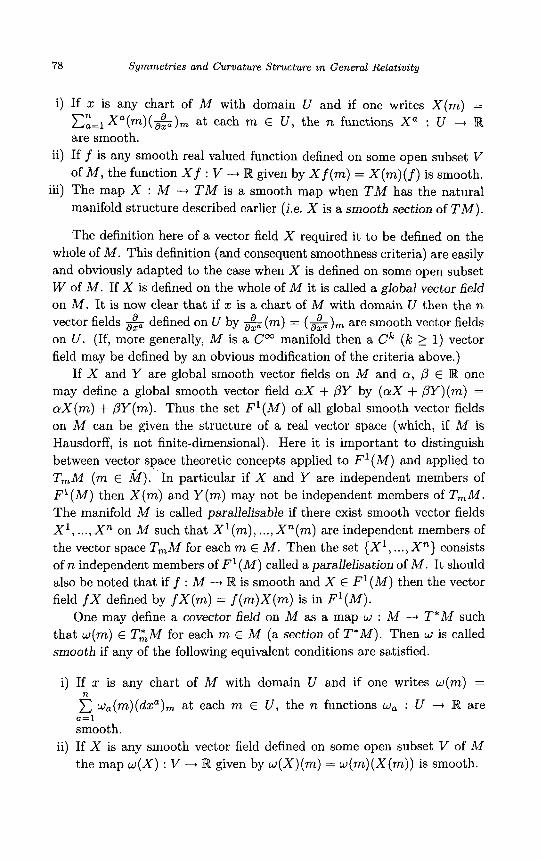
78 Symmetries and Curvature Structure in General Relativity
i) If x is any chart of M with domain U and if one writes X ( m ) =
~ ~ = l X a ( m ) ( & ) m at each m E U , the n functions X a : U 4 R are smooth.
ii) If f is any smooth real valued function defined on some open subset V of M , the function X f : V --+ W given by X f ( m ) = X ( m ) ( f ) is smooth.
iii) The map X : M --+ T M is a smooth map when T M has the natural manifold structure described earlier (i.e. X is a smooth section of T M ) .
The definition here of a vector field X required it to be defined on the whole of M . This definition (and consequent smoothness criteria) are easily and obviously adapted to the case when X is defined on some open subset W of M . If X is defined on the whole of M it is called a global vector field on M . It is now clear that if x is a chart of M with domain U then the n vector fields & defined on U by & (m) = ( &)m are smooth vector fields on U . (If, more generally, M is a C" manifold then a Ck ( I c 2 1) vector field may be defined by an obvious modification of the criteria above.)
If X and Y are global smooth vector fields on M and a, P E W one may define a global smooth vector field crX + PY by (ax + PY)(m) =
crX(m) + PY(m). Thus the set F 1 ( M ) of all global smooth vector fields on M can be given the structure of a real vector space (which, if M is Hausdorff, is not finite-dimensional). Here it is important to distinguish between vector space theoretic concepts applied to F 1 ( M ) and applied to TmM (m E &I).' In particular if X and Y are independent members of F 1 ( M ) then X ( m ) and Y ( m ) may not be independent members of T,M. The manifold M is called parallelisable if there exist smooth vector fields X 1 , ..., X" on M such that X 1 ( m ) , ..., X n ( m ) are independent members of the vector space T,M for each m E M . Then the set { X ' , ..., X n } consists of n independent members of F1 ( M ) called a parallelisation of M . It should also be noted that if f : M -+ W is smooth and X E F 1 ( M ) then the vector field f X defined by f X ( m ) = f ( m ) X ( m ) is in F 1 ( M ) .
One may define a covector field on M as a map w : M --+ T * M such that w ( m ) E TAM for each m E M (a section of T * M ) . Then w is called smooth if any of the following equivalent conditions are satisfied.
i) If z is any chart of M with domain U and if one writes w ( m ) =
C w a ( m ) ( d x a ) , at each m E U , the n functions wa : U + R are
smooth. ii) If X is any smooth vector field defined on some open subset V of M
the map w ( X ) : V 4 R given by w ( X ) ( m ) = w ( m ) ( X ( m ) ) is smooth.
n
a=l
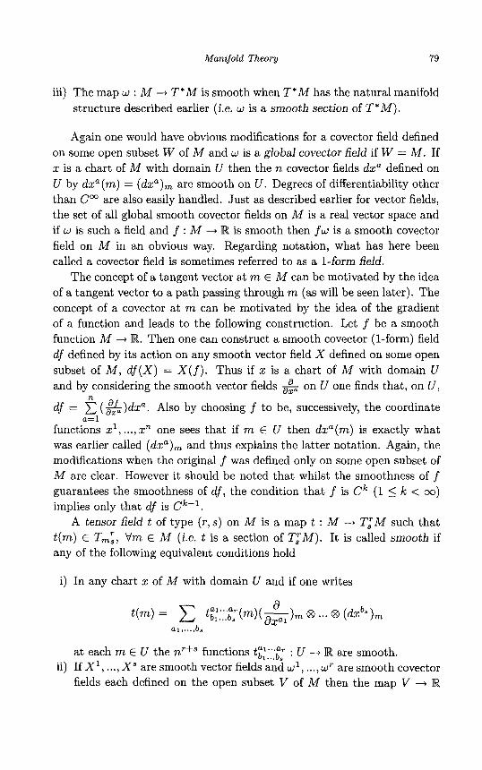
Manifold Theory 79
iii) The map w : M --+ T * M is smooth when T * M has the natural manifold structure described earlier (i.e. w is a smooth section of T * M ) .
Again one would have obvious modifications for a covector field defined on some open subset W of M and w is a global covector field if W = M . If x is a chart of M with domain U then the n covector fields dx" defined on U by d z " ( m ) = ( d z a ) m are smooth on U . Degrees of differentiability other than C" are also easily handled. Just as described earlier for vector fields, the set of all global smooth covector fields on M is a real vector space and if w is such a field and f : M -+ R is smooth then f w is a smooth covector field on M in an obvious way. Regarding notation, what has here been called a covector field is sometimes referred to as a 1-form field.
The concept of a tangent vector at m E M can be motivated by the idea of a tangent vector to a path passing through m (as will be seen later). The concept of a covector at m can be motivated by the idea of the gradient of a function and leads to the following construction. Let f be a smooth function M -+ R. Then one can construct a smooth covector (1-form) field df defined by its action on any smooth vector field X defined on some open subset of M , d f ( X ) = X ( f ) . Thus if z is a chart of M with domain U and by considering the smooth vector fields & on U one finds that, on U ,
n
n = l df = ( %)dx" . Also by choosing f to be, successively, the coordinate
_ _ functions d, ..., xn one sees that if m E U then d x " ( m ) is exactly what was earlier called ( d x a ) m and thus explains the latter notation. Again, the modifications when the original f was defined only on some open subset of M are clear. However it should be noted that whilst the smoothness o f f guarantees the smoothness of d f , the condition that f is Ck (1 5 Ic < cm) implies only that df is C"'.
A tensor field t of type (r , s) on M is a map t : M -+ T,'M such that t(m) E TmL, Vm E M (i.e. t is a section of T,'M). It is called smooth if any of the following equivalent conditions hold
i) In any chart x of M with domain U and if one writes
at each m E U the nr+' functions tE::;;b",p : U -+ R are smooth. ii) If X ' , ..., X " are smooth vector fields and w l , ..., wr are smooth covector
fields each defined on the open subset V of M then the map V + R
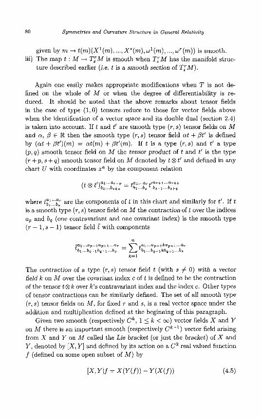
80 Symmetries and Curvature Structure in General Relativity
given by m .--) t(m)(X'(m), ..., X s ( m ) , w l ( m ) , ..., ~ ' ( m ) ) is smooth. iii) The map t : M -+ T,TM is smooth when T,TM has the manifold struc-
ture described earlier (i.e. t is a smooth section of T,TM).
Again one easily makes appropriate modifications when T is not de- fined on the whole of M or when the degree of differentiability is re- duced. It should be noted that the above remarks about tensor fields in the case of type ( 1 , O ) tensors reduce to those for vector fields above when the identification of a vector space and its double dual (section 2.4) is taken into account. If t and t' are smooth type (T , s) tensor fields on M and a, P E IR then the smooth type (r , s) tensor field at + Pt' is defined by (at + pt')(m) = at(m) + Pt'(m). If t is a type ( T , s ) and tl a type ( p , q ) smooth tensor field on M the tensor product of t and tl is the type ( r + p , s + q ) smooth tensor field on M denoted by t @ t1 and defined in any chart U with coordinates xa by the component relation
where tE:;;;b",' are the components o f t in this chart and similarly for t'. If t is a smooth type ( T , s) tensor field on M the contraction of t over the indices ap and b, (one contravariant and one covariant index) is the smooth type (T - 1, s - 1) tensor field f with components
n -a1 ... aP-l ap+l ... a , - C t a l ... a p - 1 ka,+l.. .a, tbl...b,-lb,+l...b, - bl . . .b,-l kb,+l.. .b8
k=l
The contraction of a type ( r , s ) tensor field t (with s # 0) with a vector field k on M over the covariant index c o f t is defined to be the contraction of the tensor t @ k over k's contravariant index and the index c. Other types of tensor contractions can be similarly defined. The set of all smooth type (r , s) tensor fields on M , for fixed r and s, is a real vector space under the addition and multiplication defined at the beginning of this paragraph.
Given two smooth (respectively C k , 1 5 k < co) vector fields X and Y on M there is an important smooth (respectively C"') vector field arising from X and Y on M called the Lie bracket (or just the bracket) of X and Y, denoted by [X, Y] and defined by its action on a C2 real valued function f (defined on some open subset of M ) by
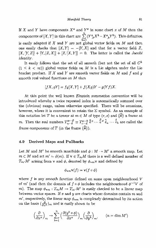
Manifold Theory 81
If X and Y have components X" and Y" in some chart x of M then the
components of [ X , Y] in this chart are (Y:bXb-X",Yb). This definition
is easily adapted if X and Y are not global vector fields on M and then one easily checks that [ X , Y ] = -[Y, X ] and that for a vector field 2, [ X , [Y, Z ] ] + [Y, [Z , XI] + [Z, [ X , Y ] ] = 0. The latter is called the Jacobi iden ti ty .
It easily follows that the set of all smooth (but not the set of all Ck (1 5 k < co)) global vector fields on M is a Lie algebra under the Lie bracket product. If X and Y are smooth vector fields on M and f and g smooth real valued functions on M then
n
b=l
At this point the well known Einstein summation convention will be introduced whereby a twice repeated index is automatically summed over the (obvious) range, unless otherwise specified. There will be occasions, however, where it is convenient to retain the C symbol. As an example of this notation let T be a tensor a t m E M of type (T , s) and {g} a frame at
m. Then the real numbers T7q::f = T,4::2 c. e e e, . . . eb are called the
frame components of T (in the frame (2)).
P r 6
4.9 Derived Maps and Pullbacks
Let M and M' be smooth manifolds and 4 : M -+ M' a smooth map. Let m E M and set m' = 4(m). If v E TmM there is a well defined member of Tm, M' arising from v and 4, denoted by 4 * m ~ and defined by
where f is any smooth function defined on some open neighbourhood V of m' (and then the domain of f o 4 includes the neighbourhood 4-'V of m). The map qLrn : TmM -+ TmtM' is easily checked to be a linear map between vector spaces. If x and y are charts whose domains contain m and m', respectively, the linear map &,,, is completely determined by its action on the basis ( &)m and is easily shown to be
82 Symmetries and Curvature Structure in General Relativity
where the matrix (-)m is the Jacobian of the coordinate representative y o 4 o 2-l of 4 at m and its rank is called the rank of 4 at m. This rank is clearly independent of the charts x and y. The map q5*m is called the derived linear function of 4 at m or the differential of q5 at m. If MI’ is another smooth manifold and 4’ : M’ -+ MI’ is smooth then (4’0q5)*~ = $’*m,oq5*m.
With 4 : M -+ M‘ as above one also has a natural map q5* : T M --+ TM’ defined by v -+ 4*v = q 5 * m ~ where v E TmM. This map is called the differential of 4 and is a smooth map between the manifolds T M and T M ‘ . With 4‘ : M’ -+ M” as above, it is clear that (4‘ o q5)* = $’* o &.
With q5 as above and f : M’ --+ R smooth define a smooth map +* f : M -+ R by qY f = f o 4, called the pullback of f under 4. Now let t be a type (0,s) tensor at m’ = $(m). Then one can construct a type (0,s) tensor at m, denoted by q5kt and called the pullback o f t under 4, by
4kt(vi, ... vs) = t ( 4 * m ( V 1 ) , ..‘> 4*m(Vs) )
for v1, ..., vs E TmM. This construction enables one to give an equivalent definition of the map 4*m : TmM -+ TmtM’ in that for v E TmM one defines q ! * m ~ by its action on a member w of Tk,M’ by
4*mV(w) = v(4kw)
This is easily checked to be equivalent to the original one and, further, allows one to push forward tensors of type (T , 0). More precisely if t is a tensor of type (T, 0) at m E M one defines a type (T , 0) tensor at m’ called the pushforward $*,t of t under 4 by
+*mt(wlr .* . ,wr) = t (4kw1, . . . , 4 t ~ r ) for w1, ..., wT E T;, M’. However the following difference should be noted. If t is a tensor field of type (0, s) on MI one can construct a tensor field of type (0,s) on M denoted by $*t, called the pullback of t under 4 and defined in the above notation by
(4*t)(m)(vl, ..., v,) = t(m’)(hmVi, ..., 4*mVs).
The tensor field 4*t is smooth if 4 and t are. But there is no similar construction for type (r,O) tensor fields in the “direction” M -+ M’. In particular although the differential 4* of q5 is a well defined map T M --f TMI it may not map a vector field X on M to a vector field on M’. This is because one may have ml, m2 E M with c$(ml) = +(mZ) but with 4*mlX(mi) # 4*m*X(m2).
Manifold Theory 83
Suppose now that $ : M -+ M' is a smooth diffeomorphism. Then the situation is much nicer. In fact if t is any smooth type (T , s) tensor field on M' then one has a smooth type (r, s) tensor field $*t on M defined by
$*t(m)(vl, . . . , V ~ W I , ...,w r ) =
t(m')($rn*vl, ' "1 $rn*Vs, $-':/01, $-':/wr)
for v1, ..., v, E T,M, w l , .., wr E TAM and where m' = $(m). Again $*t is called the pullback of t under $. Since $-' : M' -+ M is also a diffeomorphism one can move tensors in the opposite "direction" using $-'. Also, for $ : M -+ M' a smooth diffeomorphism and X a smooth vector field on M one has a smooth vector field $*X on M' defined by $,X(m') = $,,X(m) for m E M and m' = $(m) E M' [21]. In particular, if X and Y are smooth vector fields, then [qLX, qLY] = $*[X, Y ] . Similar constructions can be done when the tensor fields and map $ are Ck (1 5 k 5 00) [all.
Returning to a smooth map 4 : M ---f M' let m E M and m' = $(m). The behaviour of $ at points close to m is in a sense reflected by the action of $*m on T,M. An important case where this is made precise is in the inverse function theorem for manifolds [19].
Theorem 4.5 Let M and M' be smooth manifolds and let 4 : M -+ M' be smooth. If
m E M then 4*m is a vector space isomorphism TmM --$ Trnl M' z f and only i f there exists an open nezghbourhood U of m in M such that the restriction $1" of $ to U is a daffeomorphism from the open subset U of M onto an open subset U' of M' containing m'.
The Inverse Function Theorem for Manifolds
The proof follows from the inverse function theorem given in section 4.2 for Rn. If the conclusions of the theorem hold then M and M' have the same dimension.
4.10 Integral Curves of Vector Fields
Let M be a smooth n-dimensional manifold. A (smooth) curve or path in M is a smooth map c : I + M where I is an open interval of R. Let t be the identity chart on R, m E M and x a chart in M whose domain U contains m and intersects the range of c non- trivially. Then c, restricted to U , is often described by its component functions c"(t) where ca = xa o c and t may be restricted to some open subset of I . Often, no distinction is
84 Symmetries and Curvature Stmcture in General Relativity
drawn between the image of the curve c in M , c(I), and the curve c itself (and a member of c(I) is said to be on c). However, the map c contains more information, that is, its precise dependence on t , and to indicate this dependence t is referred to as the parameter of the curve. If t o is in the domain of the functions C" the member ($$)to(-&)c(to) of Tc(to)M with components ($$)to in the chart x is called the tangent vector (or said to be tangent) to the curve c at c(t0). To show this is a member of Tc(to)M one must check that the change in its components satisfies (4.1) under a change of coordinates in M . This is easily done but will be achieved in a coordinate independent way below. Now suppose that J is another open interval of R and f : J -+ I is a bijective map such that f and f are each smooth and where the derivative of f is nowhere zero. Define the curve c' in M by c' = co f. Then c and c' have the same range in M but, in general, have different parameters and c' is called a reparametrisation of c. The tangent vectors to c and c' at the same point m = c(t0) = c'(t'0) (where f(t '0) = t o ) differ by a (non-zero) multiple ( g)tto as is easily checked.
Let & be the vector field on R corresponding to the identity chart t . For the curve c in M define the map C = c* o &, so that 6 : I --f T M is a curve in T M , that is, it associates with each to E I a vector at c(t0) in M . This vector is precisely the tangent vector to the curve c at c(t0) since from section 4.9
d d d(x" o c) a C ( t 0 ) = (c* 0 at> (to) = c* (-) dt t o = ( dt ) t o (a,-> c( to)
Now let X be a smooth vector field on M . A curve c in M is called an integral curve of X if its tangent vector at any point of the curve equals the value of X at that point, that is, if for each to in the domain of c, C(t0) = X(c(t0)) or, equivalently, if C = X o c. If the domain of an integral curve c of X contains 0 E R, c is called an integral curve of x starting from m = c(0). Finding integral curves involves solving first order differential equations. In fact, within a chart domain U , if X = Xa& for smooth functions X" : U + R, a curve c is an integral curve of X if
(4.6) d d dt -[c"(t)] = dt[x"(C(t))] = Xa(x1(C(t)), ' " 1 xc"(c(t)))
an expression which is often loosely written as = Xa. The arbitrary constant that occurs in solving first order equations such as (4.6) can, in general, be loosely identified with the choice of starting point along a par- ticular integral curve of X . In fact, if c : I -+ A4 is an integral curve of X
Manifold Theory 85
where 0 E I (and so c starts from c(0) = m) and if to E I let f : R -+ R denote the translation t 4 t + t o . Then it can be checked that c’ = c o f is also an integral curve of X with domain f - l ( I ) starting from c’(0) = c(t0).
An important result regarding the existence of integral curves of a given smooth vector field on M can now be stated [19].
Theorem 4.6 Let X be a smooth vector field on M . Then given any mo E M there exists an open neighbourhood U of mo and an open interval I of R containing 0 such that there is an integral cuwe of X with domain I starting from any point m E U . Any other integral curve of X starting from m coincides with this curve on some neighbourhood of 0 .
Let X be a smooth vector field on M and suppose c1 and c2 are integral curves of X with domains 1 1 and I2 each of which contains 0 and which start from the same point of M . Then c1 and c2 need not coincide on I1 n I z (an example being easily constructed - see, e.g. [19]). However, c1 and c2 will coincide on I1 n I2 if M is Hausdorff [19]. For such manifolds the union of the domains of all integral curves of X which start from a given point m E M is an open interval of R containing 0 on which is defined an integral curve of X called the maximal integral curve of X starting from m. Again, with M Hausdorff, if the domain of the maximal integral curve of a smooth vector field X through any point m E M is always R then X is called complete.
There is an instructive geometrical interpretation of the derived linear function which may now be briefly commented on. Let M and MI be smooth manifolds, q5 : M -+ M’ a smooth map and c : I 4 M a smooth curve in M . Then 4 o c : I -+ MI is a smooth curve in MI. Further one may compute (q5 0 c) to find
thus showing that if v E TmM is tangent to the curve c a t m E M then q 5 * m ~ is tangent to the curve 4 o c at q5(m) E M’.
4.11 Submanifolds
In this section the important idea of a submanifold of a manifold is dis- cussed. Let M be a smooth manifold of dimension n and M’ a subset of M . The requirement that M’ be a (smooth) submanifold of M , roughly speaking, consists of two points: (i) that MI be a (smooth) manifold in its

86 Symmetries and Curvature Structure in General Relativity
own right and (ii) that it be contained in M in a smooth way. One further definition is required to achieve this. Let a and M be smooth manifolds of dimensions f i and n and let q5 : M --t M be smooth. The map q5 is called an immersion if for each m E &I the rank of q5 at m equals f i , that is, the dimension of (and so necessarily q5*fi is injective for each m E a and d i m a _< dimM). Now, returning to the original manifold M and subset M’ of M , suppose M‘ can be given a manifold structure in such a way that the natural inclusion map i : M’ 4 M is an immersion. Then M’ is called a submanifold of M (and necessarily dim M’ 5 dim M ) .
There are a number of points regarding submanifolds which should be discussed. It will be recalled that a subset of a group (or a vector or topo- logical space) can be a subgroup (or a vector or topological subspace) in at most one way since its structure is imposed upon it by the containing group (or vector or topological space). However, the definition of the submani- fold M’ above contained no such imposition on it from M other than the requirement that i be an immersion. One consequence of this weakening of the hold of the mother set over its subset is that often a subset M’ of A4 can be given the structure of a submanifold of M in more than one way. Furthermore, different submanifold structures on the subset M’ are not necessarily of the same dimension. Thus one should be careful about pre- supposing that a particular submanifold structure for a subset M‘ of M is in any sense special. Next, if the subset M’ has a submanifold structure then it has a natural topology arising from that structure as described earlier. But M’ also has a natural topology arising from the fact that it is a subset of M and thus inherits subspace topology from the natural topology on M which arises from the latter’s manifold structure. These two topologies are not necessarily equal. Of course, the map i : M‘ + M , being smooth, is continuous (when M’ and M have their respective manifold topologies) and it easily follows that any subset U of M’ which is open in subspace topology on M’ is open in the manifold topology on M‘ but the converse may fail. It may at this point seem prudent to strengthen the definition of submanifold in order to force the equality of these topologies. However, submanifolds, as defined above, occur naturally in many areas of manifold theory and so the original definition will be retained (cf. the earlier remarks concerning the Hausdorff property for manifolds). A submanifold M’ of M for which the above two topologies coincide is sufficiently special to be distinguished by a name and is called (following 1191) a regular submanifold of M . How- ever it should be noted that this nomenclature is by no means universal. In fact, the terms immersed and embedded submanifolds are sometimes
Manifold Theory 87
used, respectively, for what are here called submanifolds and regular sub- manifolds. A submanifold of M which is a closed subset of M is called a closed submanifold of M . Topological statements about submanifolds will always refer to their manifold topologies (and may differ from topological statements about them as subspaces of their containing manifold).
Some examples and properties of submanifolds can now be given for which [19] is a general reference.
i) Let U be an open subset of M and i : U + M the inclusion map. If x is a chart of M with domain V C U then x o i is a chart for U . These charts are easily shown to lead to a natural smooth manifold structure for U making it a submanifold of M of the same dimension as M and then U is called an open submanifold of M . An open submanifold of M is necessarily regular and any submanifold of M with dimension equal to that of M is necessarily an open submanifold of M . As an example, use of the determinant function shows that GL(n,R) is an open submanifold of MnR.
ii) The set MnR and its subsets of symmetric and skew-symmetric mem- bers were each given manifold structures in section 4.3. With these structures the latter two subsets are regular submanifolds of the mani- fold MnR.
iii) If V is an n-dimensional real vector space and W an m-dimensional subspace of V then W and V acquire natural smooth manifold struc- tures of dimension n and m, respectively, (example (i) of section 4.3) and then W is an m-dimensional regular closed submanifold of V.
iv) If m E M and T,M is given its natural manifold structure as a real vec- tor space then it becomes an n-dimensional closed regular submanifold of T M .
v) Let M and M be smooth manifolds of dimensions n and f i , respectively, (n > f i ) and let f : M -+ M be smooth. Let f i E M and suppose f has rank f i at each point of the subset f - l { f i } = {m E M : f (m) = f i } = M' of M . Then M' can be given the structure of a closed regular submanifold of M of dimension n - f i . A special case of this occurs when = R (and f i = 1) and then M' is an (n - 1)-dimensional hypersurface of M . In this case an obvious choice of f reveals that S" = {x E R n f l : Cy'; x! = 1) is an n-dimensional closed regular submanifold of Rn+'.
vi) If M I , M2, M'1 , M'2 are smooth manifolds with M'1 a submanifold of MI and M'2 a submanifold of M2 then the product manifold M'1 x M'2
88 Symmetries and Curvature Structure in General Relativity
is a submanifold of M I x M2. The result is still true if submanifold is replaced throughout by regular submanifold.
vii) Suppose M , M I and M2 are smooth manifolds with M2 g M I C M . If M2 is a submanifold of M I and M I is a submanifold of M then M2 is a submanifold of M . The same is true if submanifold is everywhere replaced by regular submanifold.
viii) If a subset M’ of a smooth manifold M admits the structure of a regular submanifold of M of dimension n’ then M’ admits no other submanifold structure of dimension n’ and no other regular submanifold structure of any dimension.
ix) If M’ is a regular submanifold of M and M” is a submanifold of M satisfying M” & M’ then M” is a submanifold of M’.
Suppose M’ is an n‘-dimensional submanifold of M and let i : M’ --+ M be the inclusion map. If m E M’ the map i,, : T,M’ -+ T,M is an injective map whose range is an n’-dimensional subspace of T,M called the subspace of T,M tangent to M’ and its members are said to be tangent to M‘ at m. If X is a smooth vector field on M it is said to be tangent to M’ if for each m E MI, X ( m ) is tangent to MI. This is the case if and only if there exists a smooth vector field x on M‘ such that at each m E M’, i*,x(m) = X ( m ) . In this sense vector fields on M which are tangent to M’ induce a corresponding vector field on M‘. Further, if c’ is an integral curve of then c = i o c‘ is an integral curve of X on an appropriate domain.
Because of the fact that the natural topology of a submanifold need not be its topology as a subspace, some care is needed in handling submani- folds. The following theorem and remarks show the importance of regular submanifolds (see, e.g. [19]).
Theorem 4.7 Let M1 and M2 be smooth manifolds and let f : M 1 -+
M2 be smooth. Suppose MI1 and MI2 are submanifolds of M1 and M2 respectively. Then
a) the restriction of f to MI1 is a smooth map M‘1 + M2, ii) if f ( M 1 ) C M’2 and M‘2 is a regular submanifold of M2 then f is a
iii) if f (M’1) & M‘2 and if the induced map f’ : MI1 + MI2 is smooth smooth map M1 --+ M i ,
then if v E TM1 is tangent to M‘1, f+v is tangent to M’2.
In fact (i) is trivial since if i : M’1 -+ M I is the inclusion map the restriction of f to M’1 is just the map f o i. Part (ii) may fail if the word

Manifold Theory 89
regular is dropped. (But if the word regular is dropped and if the map f : M I ---f M’z is continuous then it is necessarily smooth as a well known result on immersions shows [19].) Part (iii) may fail if f’ is not smooth (but f’ is necessarily smooth if M i is a regular submanifold of Mz).
The following example exhibits some of the unexpected behaviour of non-regular submanifolds alluded to in the above results. Let M = R3 with its usual smooth manifold structure and let S be the subset z = 0 of M . The set S can be given the following two distinct structures as a submanifold of M . Firstly S may be given a natural structure as a smooth 2-dimensional manifold MI diffeomorphic to R2. In the standard global charts the inclusion map i : MI -+ M is (z,y) + (z,y,O). Secondly, for each y E W define the map lCly : (z,y,O) -+ 2. Each lClY is a chart for S and these charts give rise to a l-dimensional manifold structure for S ( c f . example (vii), section 4.3). The resulting manifold is denoted by MI’ and the inclusion map M” -+ M in the domain of the chart ?,by is z -+ (z, y, 0). It is then easy to check that MI and M‘l are each submanifolds of M , the former being regular (and the latter, by consideration of its chart domains, clearly not). Now the inclusion map i : MI -+ M given above is a smooth map and its range is equal to the submanifold MI’. But i is not a smooth (or even continuous) map M’ 3 M” ( c f . part (ii) of theorem 4.7). Also this map i : MI t M“ can be regarded as the restriction to MI of the (smooth) identity map M -+ M . Now let m E MI and let v E TmM be the tangent vector with components (1,1,0) in the standard chart on M . Thus v is tangent to MI at m but i+,v is not tangent to M“ at m. (Since i : M -+ M is the identity map, i,, is the identity map TmM -+ TmM for each m E M and, in the above coordinates, members of T,M tangent to M” have the form (a, 0,O) (a E W) ( c f . part (iii) of theorem 4.7).
The above example shows, in particular, that a subset of a manifold can sometimes be given different structures as a submanifold of M . However, it follows from example (viii) of this section that if one has a topological subspace MI of M and one wishes to find a submanifold structure for MI whose corresponding topology coincides with the subspace topology then there is at most one such structure.
Some topological properties of submanifolds are contained in the follow- ing theorem.
Theorem 4.8 Let M be a smooth manifold and MI a submanifold of M .
i) If MI is compact its underlying set is a compact subset of M (and M’ is necessarily regular i f M is Hausdorff).
90 Symmetries and Curvature Structure in General Relativity
i i) I f M' is connected its underlying subset is a connected subset of M . iii) I f M is Hausdorff then MI is Hausdorff. iv) I f M is second countable and M' is either a connected or a regular
submanifold then M' is second countable. v) Any component of M is a connected open submanifold of M .
vi) I f M' is regular and dim M' < dim M = n (or, equivalently, MI is regular and is not an open submanifold of M ) then M' is not a dense subset of M and M \ MI is a dense subset of M .
Proof. The proofs of the first part of (i) and of (ii), (iii), (v) and the second option in (iv) are clear. The proof of the second part of (i) uses the straightforward result that a continuous bijective map from a compact topological space to a Hausdorff topological space is a homeomorphism (section 3.8). The proof of the first option in (iv) and the first part of (vi) can be found in [19]. For the last part of (vi) let U be an open subset of M such that 0 # U C MI. Then U is an open submanifold of M and dim U = n. Also, since U C M' and M' is regular, U is a submanifold of M' and the contradiction dimM' = n follows (see result (ix) of this section)Ki
The concept of a submanifold enables one to ask the question whether any n-dimensional manifold M is essentially just a regular submanifold of RN (with its usual manifold structure) for some N . Clearly the answer is no without (at least) the clauses that M be second countable and Hausdorff as theorem 4.8 shows. Some years ago Whitney [26] showed that if M is second countable and Hausdorff then M is diffeomorphic to a regular submanifold of
If M' is a submanifold of M the fact that the inclusion map i : MI + M is an immersion leads to the following result which links the charts in M' and M [19].
Theorem 4.9 Let M' be an n'-dimensional submanifold of the n- dimensional manifold M with inclusion i : M' + M and let m E MI. Then there exist charts x' in M' and x in M whose domains U' and U each con- tain m such that the corresponding coordinate representative x o i o x'-l of i is just the map (z1 , ..., znt) -+ ( z l , ..., zn', 0 , ..., 0 ) f rom some open subset of R"' into R". I n addition if M' is regular, one can choose U and U' such that U' = U n MI.
The proof of the first part is a standard property of immersions. For the final sentence one can use the continuity of i to see that i- 'U is open and hence that one can restrict U' so that U' C U . Then since M' is
Manifold Theory 91
regular there is an open subset W in M such that U‘ = M’ n W . Thus by restricting U to U n W one has M’ n (U n W ) = U’ n U = U’ to complete the result.
There is another type of submanifold which is intermediate between a general submanifold and a regular one and which will be of use later. It can be motivated by pointing out that the potential failure of theorem 4.7(ii) when M i is not regular is an irritating feature of such submanifolds. Let M’ be a submanifold of a smooth manifold M . Then M’ is called a leaf (of M ) [27] if it is connected and if whenever A is a locally connected topological space and f : A -+ M a continuous map whose range lies inside M’ then the associated map A -+ M’ is continuous. The conclusion of theorem 4.7(ii) now holds if “regular submanifold” is replaced by “leaf” in that if MI is a smooth manifold and f : M I -+ M is a smooth map whose range lies in the leaf M‘ of M then the associated map M1 -+ M‘ is continuous (theorem 4.3(i)) and hence smooth (see the remark following theorem 4.7). Just as for regular submanifolds, if a subset of M admits the structure of a leaf of M , then this structure is unique. It is remarked that a (connected) submanifold need not be a leaf and a leaf need not be a regular submanifold. In fact the so called “irrational wrap” on the torus S1 x S1 (see, e.g. [22]) is a leaf [27] but not a regular submanifold of it whereas the (connected) “figure eight” submanifold of R2 (see, e.g. [19]) is easily seen not to be a leaf.
If M I and M2 are smooth manifolds of dimension m and n, respectively, let M be the (m + n)-dimensional smooth manifold given by M = M I x MZ and p1 and pa the usual (smooth) projections. Then, for each a E MI, b E M2 the subsets bu1 = ((m1,b) : rnl E M I } and a a 2 = { ( a , m ~ ) : m2 E Mz} can be given the structure of regular submanifolds of M1 x M2 with each b f i l (respectively, a u 2 ) diffeomorphic to M1 (respectively, M z ) . The map f : T(M1 x M z ) -+ TM1 x TM2 given by f = ( p l * , p 2 , ) can be shown to be a diffeomorphism [I91 and then if X is a smooth vector field and 01 the zero vector field on M1 (and similarly for Y and 0 2 on M z ) , f 0 ( X , 0 2 ) and f -’ o (01 , Y) are, in an obvious notation, smooth vector fields on M I x MZ tangent, respectively, to each ba1 and to each aM2.
This section is concluded by remarking that, with the above notation, tensors of type ( 0 , ~ ) on M may be pulled back to M’ using the map i’.

92 Symmetries and Curvature Structure in General Relativity
4.12 Quotient Manifolds
Let M and M' be manifolds and f : M -+ M' be a smooth map. Then f is called a submersion if at each m E M , rank f = dim M' (and necessarily dim M' 5 dim M and f*m is surjective for each m E M ) . The projection maps pi : R" -+ R are simple examples of submersions when R" and R have their standard manifold structures.
Now let - be an equivalence relation on M and let M / - denote the associated quotient set. If M / - can be given a manifold structure such that the natural map p : M -+ M / -, which sends m E M to the equivalence class in M / - containing m, is a submersion then M / - is called a quotient manifold of M . For example, the equivalence relation - on R" given by ( 2 1 , ..., xn) - ( X I ' , ..., x'") if xi = xli for a particular i, (1 5 i 5 n) gives rise to the quotient set M / - = R. When R has its standard manifold structure the associated natural map M -+ M / - is just pi, which is then a submersion, and so M / - is a quotient manifold of R".
Although conceptually more difficult than a submanifold structure, a quotient manifold structure has some simpler mathematical properties. For example [19], the topology arising on a quotient manifold M / - from its manifold structure is the same as the quotient topology on M / - arising from M . Also, if a quotient set M / N admits the structure of a quotient manifold then it does so in only one way. However, a quotient manifold M / - of a Hausdorff manifold M may not be Hausdorff (cf. a remark in section 4.5).
4.13 Distributions
A vector field on a manifold M selects a member of TmM at each m E M . Sometimes there naturally arises on M not a well defined vector field but rather a well defined direction field, that is, a well defined 1-dimensional subspace of T,M for each m E M . More generally, one may have a well defined r-dimensional subspace of TmM at each m E M picked out by some construction on M . This idea leads to the concept of a distribution on M (sometimes referred to as a distribution in the sense of fiobenius to distinguish it from other types of distributions). A distribution is essentially the selection of an r-dimensional subspace of T,M for each m E M (and with r independent of m E M ) in a smooth manner. To be more precise, an r-dimensional distribution on M is a map D which associates with each
Manafold Theory 93
m E M an r-dimensional subspace of T,M (0 < T 5 n) such that for each m E M there is an open neighbourhood U of m and r smooth vector fields X1 , . . . , X , defined on U such that X1 (p), . . ., X , ( p ) span D(p) for each p E u.
It is clear in this definition how the smoothness of D is provided by the fitting of the vector fields X I , ..., X , to D.
Because of the constancy of r and the smoothness of X I , ..., X , one might ask if there exist, locally, r-dimensional submanifolds of M in which these vector fields lie (i.e. to which they are tangent). The answer in general is no and it is, therefore, of importance to have a theorem saying precisely when such submanifolds exist in terms of some property of the distribution. Let D be an r-dimensional distribution on M . Then a submanifold M‘ of M is an integral manifold of D if the natural inclusion map i : M‘ -+ M satisfies the condition that the range of the map i,, : T,M’ 4 T,M is exactly D ( m ) for each m E M’, that is, D ( m ) is the subspace of T,M tangent to M’. Thus if M’ exists it is necessarily r-dimensional. A dis- tribution D is then called integrable if every m E M is contained in an integral manifold of D. Also, a smooth vector field X on M (or some open subset of M ) is said to belong to a distribution D if X ( m ) E D ( m ) for each m in the domain of X . It follows that if X belongs to D and if M’ is an integral manifold of D then there exists a smooth vector field X’ on M’ (or some open subset of M’) such that at each m E M’ i*,X’(m) = X ( m ) (i.e. X is tangent to M’). The well known theorem due to F’robenius (see, e.g. [19]) which decides when a distribution D is integrable can now be stated and is done so in terms of a condition on vector fields like X1 , ..., X , in the first paragraph of this section which belong to D and span it at each point of the appropriate domain.
Theorem 4.10 (F’robenius) Let M be a smooth manifold and D an r-dimensional distribution on M .
Then D is integrable if and only if [ X , Y ] belongs to D whenever X and Y belong to D , where X and Y are smooth vector fields on some open subset of M . (This latter condition on D is expressed by saying D is involutive)
An alternative, useful version of this theorem arises in the following situation. Let X I , . . . , X , be T smooth vector fields defined on M with the property that a t any point m E M , X l ( m ) , . . . , X r ( m ) are independent members of T, M (so necessarily T 5 dim M ) . This set of vector fields leads to an r-dimensional distribution D on M (called the distribution spanned by (or arising from) X I , . . . , X,) which associates with m E M the subspace
94 Symmetries and Curvature Structure an General Relativity
of T,M spanned by X I (m), . . . , X,(m) (and then X I , . . . , X , belong to D ) . One asks if these vector fields have the surface forming condition namely that each m E M lies in a (necessarily r-dimensional) submanifold M’ of M such that the subspace of T,M tangent to M’ is precisely the span of { X , ( m ) , . . . , X , ( m ) } , that is, of D ( m ) (ie. D is integrable).
Theorem 4.11 Let M be a smooth manifold of dimension n and let X I , . . . , X,. be smooth global vector fields on M (r 5 n) such that X l ( m ) , . . . , X r ( m ) are independent members of T,M for each m E M . Then the distribution D spanned by these vector fields is integrable if and only if there exists smooth functions ufj on M such that these vector fields satisfy
r
[ X i , X j ] = C U & X , (1 I i , j I T ) (4.7) k= 1
Proof. Using (4.7), the properties of the Lie bracket and theorem 4.10 the theorem is proved provided that whenever X is a smooth vector field
on some open subset W of M belonging to D , so that X = C aiXi , for
functions C Y ~ : W + R then these functions are smooth. To establish this let x be a chart of M whose domain U W contains m E M . Then, in components, one has X a = ELl a i X f and the matrix X f has rank r at each point of U . After (possibly) renumbering the coordinate functions one may assume that the r x r matrix X f (1 5 i , u I r ) is non-singular at m and hence on some open coordinate domain V G U with coordinates xa (see section 3.11). Thus in V
r
i= 1
Cramer’s rule then gives the unique solution for each of the ayi and which are thus smooth since X and X I , ..., X r are. This completes the proof. 0
Some other useful results can be collected together in the next theorem (see, e.g. [19]).
Theorem 4.12 m E M .
Let M be a smooth manifold of dimension n and let
Manifold Theory 95
a) If X is a smooth vector field on M and X ( m ) # 0 there exists a chart x whose domain U contains m and such that, in U , X has components x1 = 1 , x 2 = . . . = X" = o (i.e. x = & on u).
ii) If X I , . . . , X , are smooth vector fields on M such that X , ( m ) , . . . , X , ( m ) are independent members of T,M for each m E M and also [ X i , X j ] = 0 (1 5 i , j 5 r ) then there exists a chart x with domain U containing m in which X I = &, . . . , X , = -& .
iii) Everg l-dimensional distribution on M is integrable.
If D is an integrable distribution on M there exists through each m E M a unique maximal connected integral manifold of D. This is a connected integral manifold of D through m and is maximal in that it contains all other connected integral manifolds of D through m. It is also remarked here that a l-dimensional distribution on M is sometimes called a line element field or a field of directions on M . There are obvious geometrical comparisons to be made between integral manifolds of an (integrable) distribution and integral curves of a vector field. In fact if X is a nowhere zero vector field on a manifold M and if c : I + M is an integral curve of X then c(I) can be given the structure of a (l-dimensional) integral manifold of the l-dimensional distribution on M spanned by X [19].
The concept of a distribution D defined above required the constancy of dim D ( m ) over M . In practice, one often encounters a structure on M similar to a distribution but with this constancy of dimension dropped. To avoid possible confusion such a structure will be here called a generalised distribution and will be described less generally (but in a manner sufficient for the present purposes) in terms of a certain family of smooth vector fields on M . Let S be a real vector space of global smooth vector fields on a smooth connected paracompact manifold M under the usual addition and scalar multiplication of vector fields on M . For each m E M let S, be the subspace of TmM consisting of the values of all members of S at m, that is, S, = { X ( m ) : X E S} . The map m -+ S, is called the generalised distribution on M arising from S. The dimension of S, may vary with m (and then S is sometimes called singular). If dims, is constant over m (the non-singular case), the map m + S, is a distribution on M . Let V, denote the subset of M at each point m of which, dim S, = p (0 5 p 5 n), that is, V, = { m E M : dims, = p } . Then V, is an open subset of M (possibly empty) and one has a disjoint decomposition of M in the form
M = V, UintV,-1 U . . . U int VO U V (4.8)
96 Symmetries and Curvature Structure in General Relativity
where the disjointness of the decomposition defines the (necessarily closed) subset V . Now if U is a non-empty open subset of M contained in V it follows by disjointness that U n V, = 0. If for some m E U d i m S, =
n - 1 then (section 3.11) there exists an open neighbourhood U‘ of m such that m E U’ C U and U’ C Vn-l. But this gives the contradiction (by disjointness) that m E int Vn-l. Proceeding with this argument (i.e. using the result, from section 3.11, that u;=, v k is open for each p , 1 5 p 5 n) gives the contradiction that no point of U is in V,, Vn-l,. . ., or VO and hence U is empty. It follows that V is closed and has empty interior and is hence nowhere dense in M (section 3.3). Thus V, U int V,-l U . . . U int VO is an open dense subset of M .
With the notation of the previous paragraph one can still ask about the existence of integral and maximal integral manifolds for S where now a submanifold M’ of M is called an integral manifold of S if for each m‘ E M’ the subspace of T,) M tangent to M’ is the subspace S,l (so that the members of S are tangent to MI) and a maximal integral manifold of S if it is a connected integral manifold of S which is not properly contained in any other connected integral manifold of S. After another definition a powerful result based on the work of Hermann, Stefan and Sussman [27]-[30] which generalises the theorem of Frobenius can be stated. The vector space S will be called locally finitely generated if for each m E M there exists an open neighbourhood U of m and a finite subset X I , ..., X,. E S such that
for any X E S , X = C aiXi on U for smooth functions ai : U -, R. Now suppose S is a Lie algebra with respect to its assumed vector space structure and the Lie bracket operation (in fact, a Lie subalgebra of the Lie algebra of all smooth vector fields on M under the bracket operation).
r
i=l
Theorem 4.13 Let S be a real Lie algebra of global smooth vector fields o n a smooth connected paracompact manifold M . Then if S is locally finitely generated (including the special case when S is finite-dimensional) there exists a unique maximal integral manifold of S through each m E M for which dims, 2 1 and this integral manifold is a leaf of M .
The maximal integral manifolds guaranteed by this theorem need not be regular submanifolds of M but since they are leaves, the conclusion of theorem 4.7(ii) when M i is such a submanifold is guaranteed. It is also remarked here that in the case of a (Fkobenius) distribution the conclu- sion of theorem 4.7(ii) for M i a maximal integral manifold has been known for some time since, because M is paracompact and connected, it is sec-

Manifold Theory 97
ond countable (theorem 4.4) and since M i is connected it is also second countable (theorem 4.8(iv)). The result now follows from a result in [19].
4.14 Curves and Coverings
In chapter 3 the idea of a curve in a topological space as a certain contin- uous map was discussed whereas in this chapter the curves of importance have been smooth curves in manifolds. Similarly, the concepts of the fun- damental group and of coverings were discussed topologically, that is, using continuous maps, and one may similarly enquire about their smooth coun- terparts when applied to manifolds. This section provides a brief discussion of some of these points.
Let M be a smooth Hausdorff manifold and let p, q E M . Fkom chapter 3 a curve c in M from p to q is a continuous map c : [0,1] -+ M with c(0) = p, c(1) = q. A piecewise Ck curve ( I c 2 1) in M from p to q is a map c’ defined on the closed interval [a, b] such that c’(a) = p, c’(b) = q and such that the interval [a,b] can be divided into finitely many closed subintervals [a, sl], [ s I , s ~ ] , . . . , [s,-l,b] with a < s1 < ... < sm- l < b on each of which c’ agrees with a Ck map into M from an open interval of R containing that subinterval [19]. It is now straightforward to show that for p , q E M , the relationp N q e there exists a piecewise Ck curve from p to q, is an equivalence relation on M each equivalence class of which is open and closed in M (and hence equal to M if M is connected, equivalently, path connected from theorem 4.3(iv) [19]. Hence if one can find a (continuous) curve between two points of M one can find a piecewise Ck curve between them (and clearly conversely from the material in section 3.10). Hence the definition of path connectedness (or local path connectedness) could be stated in terms of (continuous) curves or piecewise Ck curves ( I c 2 1). In fact, if one can find a curve from p to q in M one can, by smoothing procedures, find a smooth curve from p to q and so the definition of path connectedness could be phrased in terms of smooth curves.
Since a manifold is a topological space one can discuss its fundamental group in terms of (continuous) curves. It can be shown that the results obtained are the same as if one had used piecewise smooth curves or even smooth curves together with (in the obvious sense) smooth homotopies. In fact the only new results required are, firstly, that if c is a closed curve at p then there is a smooth closed curve c’ at p which is continuously homotopic (i.e. in the sense of section 3.10) to c and, secondly, if c1 and c2 are two
98 Symmetries and Curvature Structure an General Relativity
closed smooth curves at p which are continuously homotopic to each other then they are smoothly homotopic to each other.
be smooth connected Hausdorff manifolds. Regarding them firstly as topological spaces it makes sense to ask if A?f is a covering space of M , that is, if a covering map p : M --+ M exists as described in section 3.10. Now define a smooth covering (as opposed to a covering which is a continuous map between topological spaces) p’ : M --t M as a smooth surjective map such that for each m E M there exists a con- nected open subset U containing m such that each component of p’-lU is diffeomorphic to U under (the appropriate restriction of) p’ and when these open subsets have their usual open submanifold structure. It follows that the dimensions of M and M and the rank of p’ at any m E M are equal. Next let M be a covering of M with covering map p : M 4 M (so that only the manifold topologies of M and are relevant). Then it does not necessarily follow that p is a smooth covering since p may not actually be smooth (just consider one of those sets upon which different manifold structures can be put but which have identical manifold topologies (see e.g. [19]) and consider the identity map on the set). However one does have the result that, for topological spaces M and &l and a covering p : &!L’ -+ M and given a manifold structure for M whose manifold topology equals the original topology on M , there exists a unique manifold structure for &if
whose manifold topology equals the original topology on M and for which p is a smooth covering 1181. The manifold M is called a covering manifold of M . If M is simply connected it is called the universal covering manifold of M . Every smooth connected Hausdorff manifold has a unique universal covering manifold in the sense that if and &l2 are universal covering manifolds of M with smooth covers p1 : + M and p2 : 2 2 -+ M there exists a smooth diffeomorphism h : MI --f M 2 such that p2 0 h = p l . To see this note that section 3.10 guarantees a homeomorphism h’ : 2 1 + Mz such that, as continuous maps, p2 oh‘ = p l . Now p l and p2 are immersions and a standard result [19] now shows that h and h-’ are smooth and the result follows. Further, if one defines an equivalence relation N on A? by ml N m2 p ( m 1 ) = p ( m 2 ) then any smooth connected Hausdorff mani- fold is diffeomorphic to a quotient manifold of a simply connected manifold (i.e. to hf/ -). The proof is similar to that for topological spaces in 3.10. One has a natural bijection f : M --+ &l/ N from which a natural manifold structure for i@/ N results making f a diffeomorphism. The natural map i : a + M/ N then satisfies i = f o p and is smooth with rank equal to the rank of p which equals dim fi at each point of M. Thus i is a submersion
Now let M ,

Manifold Theory 99
(section 4.12) and the result follows.
4.15 Metrics on Manifolds
From the point of view of this book one of the most important constructions on a manifold is that of a metric. Let M be a smooth manifold and let m E M . A metric a t m is an inner product on TmM, that is, a symmetric non-degenerate bilinear form on TmM. In other words, a metric at p is a symmetric type (0,2) tensor at p whose components constitute an n x n non- singular symmetric matrix at p . A smooth metric on M is a global smooth tensor field of type (0,2) on M which is a metric at m when evaluated at any m E M . If in the above definitions one replaces inner product by positive definite inner product the resulting metric on M (or metric at m E M ) is called positive definite. If, however, one replaces inner product by inner product of Lorentz signature one arrives at a (smooth) Lorentz metric on M (or at m E M ) . In fact the signature of a metric on a connected manifold M is the signature of any of the inner products representing it (it being straightforward (see section 4.16 after (4.39)) then to prove that this signature is the same a t each point of M ) . All concepts of orthogonality for a metric are as defined for inner products in section 2.5.
Let gm be a metric at m E M and let x be a chart whose domain contains m. Then at m one has (recalling the Einstein summation convention)
where the components gab (= gba) of gm in the chart x form a symmetric matrix with det(g,b) # 0. Under a change of coordinates the general law (4.4) shows that, at m, gbb = AacgcdAzb where Aab = ($$) . It now follows from section 2.5 (and, in particular, from Sylvester's law) that one may change coordinates about m so that, a t m, the matrix gbb assumes the Sylvester form (2.1) appropriate to its signature. Let gab be the matrix inverse to gab and define the (2,O) tensor gm-' = gab(&)m 8 ( G ) ~ a at m (this definition being easily shown to depend only on gm and not on the chart x in which the components were computed). A metric gm at m E M distinguishes a vector space isomorphism from TmM to its dual space TAM where, hitherto, no such natural isomorphism existed. This isomorphism, denoted by fgm (to highlight its dependence on gm) is defined by v -+
fgmv E TAM where fg,v(u) = gm(v,u) (u ,v E T m M ) . If in some chart x
m
100 Symmetries and Curnature Structure in General Relativity
whose domain contains m, v = V , ( = ) ~ , a then fgmv = (g,bUb)(dxa)m. One traditionally defines v, = gabVb so that fgmv = v,(dxa)m (and provided, of course, that no ambiguity is involved i.e. that the metric gm is understood). Thus one says that the metric gm lowers indices at m E M . The process of raising indices can be accomplished by using the map fgml : TA M -+ T, M defined for w E T$M by fg,lW(t) = g;'(w, t) (t E T A M ) and in the chart x the effect, in components, is t , + ta = gabtb. The definition of 9;' shows that gacgcb = Sg and it is then easily checked that raising and lowering indices are inverse operations. If M admits a smooth metric g then the above shows that any smooth vector field on some open subset U of M has a naturally associated covector field on U associated with it (and vice versa). If X has components X " in some chart of M contained in U then the associated covector field has components X , = gabXb in U .
One may extend index raising and lowering to general tensors. Omitting the details (which are similar to those described in the previous paragraph- see e.g. [24]) one can lower (or raise), using a given metric gm, a particular index of a type (r , s) tensor T at m turning it into a type (r - 1, s + 1) (or a type (r + 1,s - 1) tensor at m. The same symbol T would still be used for the resulting tensor. Thus, for example, one would have in components
4 Tabcd gaeTebcd, Tabcd TabCd g a e g b f T e f C d . Although the order of the u p (contravariant) indices and that of the down (covariant) indices is important there is no such significance between the ordering of up relative to down indices. In practice one does allow significance to the relative position of an up and a down index but only to indicate relative position when the up index is lowered or the down index raised.
One can always construct a metric of any signature ( r , s ) at a point m E M subject to r + s = dimM (and, indeed, one may construct a smooth metric of this signature on the domain U of any chart x of M by choosing an appropriate non-singular matrix gab and defining the metric to be gabdxa @ d x b on U ) . However, one cannot necessarily define a global smooth metric on a given manifold M . The following theorems summarise the situation in the positive definite and Lorentz cases.
Theorem 4.14 the following conditions are equivalent.
Let M be a smooth connected Hausdorff manifold. Then
a) M admits a global smooth positive definite metric. i i) M is paracompact.
iii) M is second countable. iv) M admits a partition of unity.
Manafold Theory 101
v) The manifold topology of M is metrisable.
Proof. A brief sketch of how the proof proceeds is easily given. One notes first that the equivalence of (ii), (iii) and (iv) is just the statement of theorem 4.4. Next, the existence of a partition of unity on M and the existence of local smooth positive definite metrics in the chart domains of M together allow a smooth globalising procedure to be carried out which results in a smooth global positive definite metric on M and so (i) follows from either of the equivalent conditions (ii), (iii) or (iv) [19]. If, however, (i) is assumed to hold then the metric g which arises can be used to construct the magnitude (or size) g(v,v): of any tangent vector v at any point of m. Now since M is connected there is a piecewise smooth curve c : [a,b] + M joining any two points p , q E M . Thus [a,b] can be divided up according to a = to < tl < ... < t , = b and so that c agrees with a smooth curve c, on [t,-l, t,] ( a = 1,. . . , m). The length of c is defined to be xy=l S,","_,g(v(t),v(t))fdt where v( t ) is the tangent vector to the relevant curve c,. Such lengths are non-negative real numbers and allow a map d : M x M + R to be defined where for p , q E M , d ( p , q ) is the infimum of the lengths of all piecewise smooth curves from p to q. The map d turns out to be a metric for M in the sense of section 3.2 and the consequent metric topology on M coincides with the manifold topology for M . Thus (v) follows, Finally if (v) holds then (ii) (and hence (iii) and (iv)) follow from Stone's theorem (see section 3.8) which says that any metric space is paracompact. 0
Theorem 4.15 Let M be a smooth connected paracompact n-dimensional manifold (n 2 2). Then M admits a (smooth) Lorentz metric if and only if it admits a 1-dimensional distribution.
Proof. To prove this one notes that the conditions of the theorem tc- gether with the previous theorem ensure the existence of a global smooth positive definite metric y on M . If M also admits a 1-dimensional distribu- tion then in some open coordinate neighbourhood U of any m E M there exists a smooth vector field t which spans the distribution. Clearly one may assume t is everywhere of unit size with respect to y (i.e. r ( t , t ) = 1 everywhere on U ) since y is smooth and so t is determined up to a sign at each point of U . It follows that the smooth tensor t @ t of type (2,O) is uniquely determined on U . Then by using y to lower indices one obtains a smooth type (0,2) tensor on U with components tatb ( t , = Tab$) . By covering M with such neighbourhoods and their corresponding type (0,2)
102 S y m m e t r i e s and Curvature S t ruc ture in General Re la t i v i t y
tensors the latter clearly give rise to a global type ( 0 , 2 ) tensor h on M (the ambiguity in the sign of the vector spanning the distribution at any point being cancelled in the definition of h). One then constructs the global ( 0 , 2 ) smooth tensor g = y - 2h on M which is, in fact, a smooth Lorentz metric on M . To see this let t , v1, ..., v,-1 be an orthonormal basis (with respect to y) at m E M with t spanning the distribution at m. In this basis g has components g a b = diag(-1, 1, . . . , 1) and so is in the Sylvester form for a Lorentz metric at m.
Conversely let y be a global smooth positive definite metric on M (which exists from the paracompactness of M by the last theorem) and let g be a Lorentz metric for M with signature (-1,1,. . . , 1). Let 2 be a chart whose domain contains m and using components in this chart at m consider the eigenvector-eigenvalue problem g a b k b = for k E Rn, X E C. By adjusting the chart so that y a b = dab at m and using the symmetry of g one sees (section 2.6) that all such eigenvalues are real and that g a b is diagonalisable over R. Also, det g a b < 0 and so at least one such eigenvalue, say XO, must be negative. Denote by ua a corresponding eigenvector so that at m, gab?Lb = XOyabUb. A contraction with u then shows that gabUaUb < 0. If there exists another negative eigenvalue A 1 # Xo and corresponding eigenvector v then again one finds g a b V a v b < 0 and, since XO # XI, one easily finds gabUaVb = 0. This latter equation and the previous two inequalities are easily checked to be inconsistent with the Lorentz signature of g and so there is a unique negative eigenvalue Xo(m) at m. The diagonalisability of g a b then shows that the Xo(m)-eigenspace is a 1-dimensional subspace of T,M. But Xo(m) is a simple root of the polynomial det(gab - X y a b ) = 0 at each m E M and hence depends smoothly on the smooth coefficients of the polynomial (see, e.g. [31]). Hence the numbers Xo(m) determine a global smooth function M 4 R (also denoted by XO). Now consider the global smooth tensor field A of type (1,l) defined in the domain of any chart by the components A a b = g a c ( g c b - XOycb) . At each m E M the matrix A a b
has rank n - 1 and the (n - 1)-dimensional subspaces of TmM given at each m E M in components by { A a b v b : v E T m M } give rise to a smooth (n - 1)-dimensional distribution on M [31]. The orthogonal complement with respect to g of this distribution is then itself a (1-dimensional) smooth distribution [31] and agrees with the Xo-eigenspace at each m E M . Thus M admits a 1-dimensional distribution. 0
It may be wondered whether the paracompactness clause in the pro- ceeding theorem is really necessary. It turns out that in the case of most
Manifold Theory 103
importance for this book, i.e. dim M = 4, it is in the sense that if a smooth connected Hausdorff 4-dimensional manifold admits a smooth Lorentz met- ric it is necessarily paracompact [32].
Now suppose that M is a smooth manifold admitting a metric g and let M' be a submanifold of M with inclusion i : M' -+ M . Then the pullback i*g is a smooth symmetric tensor of type (0,2) on M' but it is not necessarily a metric for M' since it may fail to be non-degenerate at some (or all) points of M'. It is, however, a standard result that if g is positive definite then i * g is a positive definite metric for M' called the metric induced on M' by g [20]. For Lorentz metrics one has the following theorem.
Theorem 4.16 Let M be a smooth manifold with Lorentz metric g of signature (-1,1, ..., 1) and let M' be a submanifold of M with inclusion i. If dimM' = dimM then M' is an open submanifold of M and i*g is a Lorentz metric for M' (the restriction of g to MI). Otherwise
a ) if for each m E M' and v E T m M , v # 0 with v tangent to MI ,
ii) if for each m E M' there exists v E TmM with v tangent to M' and g m ( v , v ) > 0 then i*g is a positive definite metric for M',
gm(v,v) < 0 then i * g is a Lorentz metric for MI.
The proof of (i) is clear since if u E TmM', u # 0 , then ( i * g ) m ( u , u) > 0. For (ii) the proof will be clear after the algebraic discussion of Lorentz metrics in the next chapter. Clearly, for a general submanifold M' of M , the nature (degenerate, positive-definite or Lorentz) of i * g will vary over MI.
A smooth manifold M together with a metric g on M is often written as the pair ( M , g ) or simply as M if g is clear. If g is positive definite, ( M , g ) or M is sometimes called Riemannian. However this notation is not universal, some authors preferring the latter term for any manifold with a metric (of arbitrary signature). Hence it will not be used in this text. If g has Lorentz signature, ( M , g ) or M is sometimes called Lorentz or Lorentzian. If M = R" and g is a smooth metric on M which in the usual global chart has components gab, where gab equals the appropriate Sylvester matrix for g , at each m E M then ( M , g) is called pseudo-Euclidean (and Euclidean if g is positive definite). If each point of M has a coordinate neighbourhood in which the metric takes constant values, as in the last sentence, it is called locally pseudo-Euclidean or locally Euclidean. If ( M , g ) and (M' , 9') are smooth manifolds with smooth metrics g and g' and if f : M -+ M'
104 Symmetries and Curvature Structure in General Relativity
is a diffeomorphism such that f*g‘ = g then f is called an isometry and ( M , g ) and (M’,g’) are then isometric. Again if ( M , g ) and (M’,g’) are manifolds with metrics let ~ = M x M’ be the smooth product manifold and i : &l -+ M , j : A? + M’ the natural projections. There is a natural smooth metric g c3 g‘ on &l defined by g 8 g’ = i*g + j*g’ and called the product of g and g’ (see e.g. [24]) and one refers to the metric product of M and MI.
A notational remark can now be made regarding metrics on mani- folds. An old classical notation often employed in relativity theory is that which describes a metric g in the domain U of a chart x by writing ds2 = gabdxadxb. Although formally similar to (4.9) it had quite a different meaning, classically, being thought of as the square of the distance between two points whose coordinate separation was dxa (at least in the positive definite case)! The modern approach to metrics given here describes them as giving size to tangent vectors. The above classical notation is still use- fully employed but only in the sense of being an alternative (possibly more picturesque) way of actually defining g in that chart.
4.16 Linear Connections and Curvature
One of the most important concepts in differential geometry and theoretical physics is that of a connection. More details will be provided in a later chapter when holonomy theory is considered. In this section the basic idea of a linear connection (sometimes shortened to connection) is considered.
A (linear) connection V on M is a map which associates with two smooth vector fields X and Y defined on open subsets U and V of M , respectively, a third smooth vector field denoted by V x Y defined on U fl V such that for smooth real valued functions f, g and a smooth vector field Z defined on appropriate open subsets of M and a , b E R
Vz(aX + b y ) = UVZX + bVzY (4.10) V f X + g Y Z = fVxZ+gVyZ (4.11)
(4.12)
where all appropriate domains are assumed to be non-empty open subsets of M . A connection as defined above will be called smooth. Rather than repeat statements about domains of definition of various constructions it will be assumed, unless stated otherwise, that they are open subsets of M or the obvious intersections of open subsets of M . It is convenient, for f
v x (f Y ) = f v x y + (X(f ))Y
Mani f ol d Theory 105
and X as above, to define V x f = X ( f ) so that (4.12) assumes a Leibniz form.
The quantity VxY is referred to as the covariant derivative of the vec- tor field Y along the vector field X (and, similarly, V x f is the covariant derivative of f along X ) . As the form of the above axioms suggest, they are an attempt to place a structure on M which allows a sensible derivative of a vector field Y along the integral curves of another vector field X to be defined. By implication one thus has the concept of a constant vector field along the integral curves of a vector field Y and, it turns out, along any smooth curve in M . Thus if M is connected (and hence path connected) one has a notion of parallel displacement or transport (movement "without change") of tangent vectors between any two points of M but along a par- ticular curve connecting these points (and which may depend on the curve chosen).
A manifold M may not admit a connection. However, any manifold admits one locally by virtue of it being locally like R". To see this let x be a chart of M with domain U and let X and Y be any smooth vector fields on U with X = X"& and Y = Y"& for smooth functions X " and Y". Then define V on the open submanifold U of M by
a a VXY = X ( Y " ) - = (YEXb)-
a X a dX" (4.13)
It is easily checked that V is a connection on U (which is dependent on the chart x). The same construction reveals a standard global linear connection on Rn from its usual global chart.
Turning to the general existence of connections on a manifold M the following theorem (see e.g. [19]) is fundamental.
Theorem 4.17 ear) connection.
Any paracompact smooth manzfold admits a smooth (lin-
The proof is similar in essence to that of theorem 4.14 for positive defi- nite metrics. One uses a partition of unity on M (which exists from theorem 4.4) to spread out the above local connections smoothly on M . Henceforth M will be assumed to be paracompact.
Let M be a (smooth paracompact) manifold which admits a connection V . There are associated with V two constructions on M of particular importance. Let X and Y be smooth vector fields and consider the smooth vector field T ( X , Y ) defined by
qx, Y ) = V X Y - vyx - [ X , Y ] (= -T(Y, X ) ) (4.14)

106 Symmetries and Curvature Structure in General Relativity
5? is called the torsion of V. All the connections considered in this text will have zero torsion in the sense that T(X, Y ) will always be the zero vector field and then the connection V is called symmetric. This will be discussed further later. Of more importance here is the curvature structure R. Let X, Y, Z be smooth vector fields and define a smooth vector field by
R(X, Y ) Z = V x ( V y 2 ) - V y ( V x 2 ) - V[x,y]Z (= -R(Y, X)Z) (4.15)
it is easily seen that R is linear in each of its arguments in the sense that, for example, for vector fields X1 and X2 and a, b E R
R(aX1+ bX2, Y ) Z = &(XI, Y)Z + bR(X2, Y ) Z (4.16)
and from (4.15) one can also show [33] that if f, g and h are smooth functions
R(fX, gY)hZ = fghR(X, Y ) Z (4.17)
The curvature structure R leads to a global type (1,3) smooth tensor field also denoted R on M called the curvature (or Riernann) tensor (associated with the connection V). To see this let m E M and let x be a chart whose domain U contains m. Let X'l, X'2, X'3 E TmM and w' E T&M be given by x ' k = X,"(&)m (Ic = 1,2,3), w' = w,(dxa)m (X,", w, E R) and extend them smoothly to U by XI, = X,"& (k = 1,2,3), w = w,dxa for smooth functions X," and w, on U . Then define
f i (m) (w ' , x'1, x'2, x'3) = [(R(&, xdx1) (w) lm (4.18)
It is straightforward to check that this definition is independent of the choice of XI, and w provided they yield X'k and w' on evaluation at m. It also follows from the definition that R is smooth. In components in U one has
(4.19)
where the smooth functions R a b c d are the curvature tensor components. By virtue of (4.15) they satisfy
d dX"
R = Rat,&- 8 dxb 8 dx" 8 dxd
R a b c d = - R a b d c (4.20)
Since V is symmetric, T = 0 and (4.14) and (4.15) give
R(X, Y)Z + R(Y, Z)X + R(2 , X)Y = 0 (4.21)
Manifold Theory 107
which in terms of components is the (algebraic) Bianchi identity
Again in the chart x with domain U define smooth functions rtc on U by the relations
(4.23)
The functions rtc are called the coefficients of the connection V in the chart x and (4.14) shows that V is symmetric if and only if qC = r:b in each coordinate domain. They are not the components of any tensor at any point of U since if y is another chart of M whose domain intersects U then by writing out (4.23) in the y coordinates, using the symbol rba, for the connection coefficients in these coordinates, one easily finds on the intersection of these coordinate domains that
(4.24)
It should be remarked at this point that if V and V are two connections on M whose coefficients are I?& and r2c in some coordinate domain U of M then the functions rgc - do define a smooth tensor field on U of type (1 ,2) . Also, if one specifies smooth functions in each domain of an atlas of M which satisfy (4.24) on the intersection of any two such domains then one has, in fact, defined a connection on M through (4.23) whose coefficients are the functions rtc. It is symmetric if and only if in each coordinate domain (and it is noted how this property is preserved by (4.24)). A convenient expression for the curvature tensor components in any chart domain can be obtained from (4.18), (4.19) and (4.23)
=
Rabcd = r&,c - r z b 3 d + r&rze - r%r:e (4.25)
Now let X be a smooth vector field. From the connection V and X one can define a type ( 1 , l ) tensor field V X on M as that unique ( 1 , l ) tensor field such that the (only possible) contraction of V X with any smooth vector field Y is the vector field V y X . Now by using (4.11), (4.12) and (4.23) one easily finds that in any coordinate domain U of M and for vector fields X and Y defined on U
(4.26)
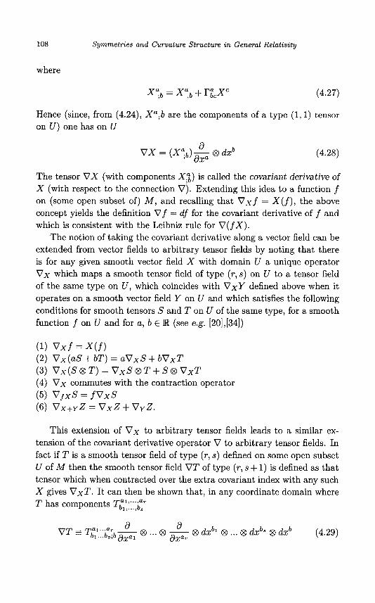
108 Symmetries and Curvature Structure in General Relativity
where
(4.27)
Hence (since, from (4.24), X a ; b are the components of a type (1,l) tensor on U ) one has on U
(4.28)
The tensor VX (with components X;) is called the covariant derivative of X (with respect to the connection V ) . Extending this idea to a function f on (some open subset of) M , and recalling that V x f = X ( f ) , the above concept yields the definition V f = df for the covariant derivative of f and which is consistent with the Leibniz rule for V ( f X).
The notion of taking the covariant derivative along a vector field can be extended from vector fields to arbitrary tensor fields by noting that there is for any given smooth vector field X with domain U a unique operator V x which maps a smooth tensor field of type (T , s) on U to a tensor field of the same type on U , which coincides with V x Y defined above when it operates on a smooth vector field Y on U and which satisfies the following conditions for smooth tensors S and T on U of the same type, for a smooth function f on U and for a , b E R (see e.g. [20],[34])
(1) V x f = X ( f ) (2) V X ( U S + bT) = UVXS + bVxT (3) V x ( S @ T ) = V x S @ T + S @ V x T (4) V X commutes with the contraction operator ( 5 ) VfXS = f V x S ( 6 ) Vx+yZ = V x Z + VyZ .
This extension of V x to arbitrary tensor fields leads to a similar ex- tension of the covariant derivative operator V to arbitrary tensor fields. In fact if T is a smooth tensor field of type (T , s) defined on some open subset U of M then the smooth tensor field VT of type (T , s + 1) is defined as that tensor which when contracted over the extra covariant index with any such X gives V x T . It can then be shown that, in any coordinate domain where T has components TE',;::;b",'
(4.29)
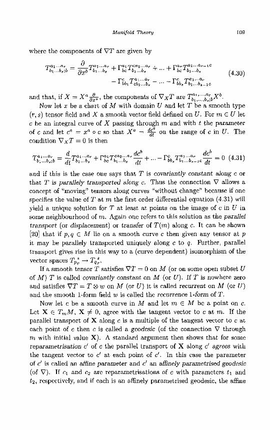
Manzfold Theory 109
where the components of VT are given by
and that, if X = X a & , the components of V x T are Tb“,’,;::;,?bXb. Now let x be a chart of M with domain U and let T be a smooth type
( T , s) tensor field and X a smooth vector field defined on U . For m E U let c be an integral curve of X passing through m and with t the parameter of c and let ca = xa o c so that X a = on the range of c in U . The condition VxT = 0 is then
= 0 (4.31) dcb dcb a1 ... a , d a l . . a , + F a 1 T c a z ... a , - + .. . - r c T a i ... a ,
Tbl...bs;b = z T b l ... b. bc b1 ... 6, d t bbs b l . . . b s - i c d t
and if this is the case one says that T is covariantly constant along c or that T is parallely transported along c. Thus the connection V allows a concept of “moving” tensors along curves “without change” because if one specifies the value of T at m the first order differential equation (4.31) will yield a unique solution for T at least at points on the image of c in U in some neighbourhood of m. Again one refers to this solution as the parallel transport (or displacement) or transfer of T(m) along c. It can be shown [20] that if p , q E M lie on a smooth curve c then given any tensor at p it may be parallely transported uniquely along c to q. Further, parallel transport gives rise in this way to a (curve dependent) isomorphism of the vector spaces Tp: + Tq:.
If a smooth tensor T satisfies VT = 0 on M (or on some open subset U of M ) T is called covariantly constant on M (or U). If T is nowhere zero and satisfies VT = T I% w on M (or U ) it is called recurrent on M (or U ) and the smooth 1-form field w is called the recurrence 1-form of T .
Now let c be a smooth curve in M and let m E M be a point on c. Let X E T,M, X # 0, agree with the tangent vector to c at m. If the parallel transport of X along c is a multiple of the tangent vector to c at each point of c then c is called a geodesic (of the connection V through m with initial value X). A standard argument then shows that for some reparametrisation c’ of c the parallel transport of X along c’ agrees with the tangent vector to c’ at each point of c’. In this case the parameter of c’ is called an affine parameter and c’ an d n e l y parametrised geodesic (of V). If c1 and cz are reparametrisations of c with parameters tl and tz, respectively, and if each is an affinely parametrised geodesic, the affine
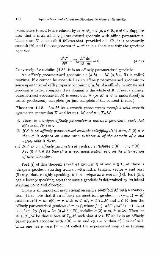
110 Symmetries and Curvature Structure in General Relativity
parameters tl and t z are related by t z = at1 + b (a , b E R, a # 0). Suppose now that c is an affinely parametrised geodesic with affine parameter t. Then since V is smooth it follows that, provided c is C1, it is necessarily smooth [20] and the components ca = xu o c in a chart z satisfy the geodesic equation
(4.32)
Conversely if c satisfies (4.32) it is an affinely parametrised geodesic. An affinely parametrised geodesic c : ( a , b) + M (a , b E R) is called
maximal if c cannot be extended as an affinely parametrised geodesic to some open interval of R properly containing (a , b). An affinely parametrised geodesic is called complete if its domain is the whole of R. If every affinely parametrised geodesic in M is complete, V (or M if V is understood) is called geodesically complete (or just complete if the context is clear).
Theorem 4.18 symmetric connection V and let m E M and v E TmM.
Let M be a smooth paracompact manifold with smooth
i ) There is a unique afinely parametrised maximal geodesic c such that c(0) = m, C(0) = v
i i) If c’ is an afinely parametrised geodesic satisfying c’(0) = m, C’(0) = v then c‘ is defined on some open subinterval of the domain of c and agrees with it there.
iii) If c‘ is an afinely parametrised geodesic satisfying c’(0) = m, C’(0) = Xv, (0 # X E R) then c‘ is a reparametrisation of c on the intersection of their domains.
Part (i) of this theorem says that given m E M and v E TmM there is always a geodesic starting from m with initial tangent vector v and part (ii) says that, roughly speaking, it is as unique as it can be [HI. Part (iii), again loosely speaking, says that such a geodesic is determined by its initial starting point and direction.
There is an important map arising on such a manifold M with a connec- tion. First note that if an affinely parametrised geodesic c : (-a,a) + M satisfies c(0) = m, C(0) = v with m E M , v E TmM and a E R then the affinely parametrised geodesic c’ = cof, where f : (-aX-l, aX-’) + (-a, a ) is defined by f(z) = Xz (0 # X E R), satisfies c’(0) = m, C’ = Xv. Then let W TmM be that subset of T,M such that if v E W and c is an affinely parametrised geodesic with c (0 ) = m and C(0) = v then c(1) is defined. Thus one has a map W + M called the exponential map at m (arising

Manifold Theory 111
from the connection) and denoted by exp, and defined by exp,v = c(1). It follows that, if tv E W , exp,(tv) = c(t) and that the maximal geodesic starting from m with initial tangent v is the map t -+ exp,(tv) for appro- priate t. The following theorem now holds [18],[19],[20].
Theorem 4.19 Let M be a smooth paracompact manifold admitting a smooth symmetric connection and let m E M . Then there exists an open subset V of T,M containing 0 and an open subset U of M containing m such that exp, : V + U is a (smooth) diffeomorphism between the obvious open submanifold stmctures on V and U .
Henceforth, the exponential map will always be understood to have an open domain and range as described in theorem 4.19.
Now let XI, ..., X, be a basis for T,M and, with the notation of the previous theorem, define a smooth map U --t Rn with components xa by xa(exp,(v)) = wa given that v = waxa. This defines a chart z for M with domain U as is easily checked. The corresponding coordinate system is called a normal coordinate system for M a t m. The coordinate expression for an affinely parametrised geodesic c in U satisfying c(0) = m and k(0) = v is then ca(t) = tva where ca = xaoc and any curve of this form is an affinely parametrised geodesic (lying in U ) . The point m is the origin of the above normal coordinate system and its coordinates are (0, ..., 0). It follows that for these normal coordinates (&), = X,. It also follows from (4.32) and the above discussion that, in these coordinates, the coefficients rtC vanish at m. Hence any m E M admits a coordinate domain in which r;c(m) = 0.
There are a number of differential identities satisfied by the curvature tensor on M arising from a (symmetric) connection V. Let z be a chart of M with domain U . Covariant differentiation of tensors on U is not necessarily commutative and a series of identities, the Ricci identities, point this out. They are given here in component form for a vector field X , a covector field w and a type (0,2) tensor field T on U . They can be derived, somewhat tediously but easily, from (4.25) and (4.30). A double covariant derivative will be denoted by two indices after the semi-colon rather than two semi-colons. Thus Xa;b;c will be written Xa;bc.
Xabc - X"b = XdRadcb (4.33)
Wa;bc - wa;cb = W d R d abc (4.34)
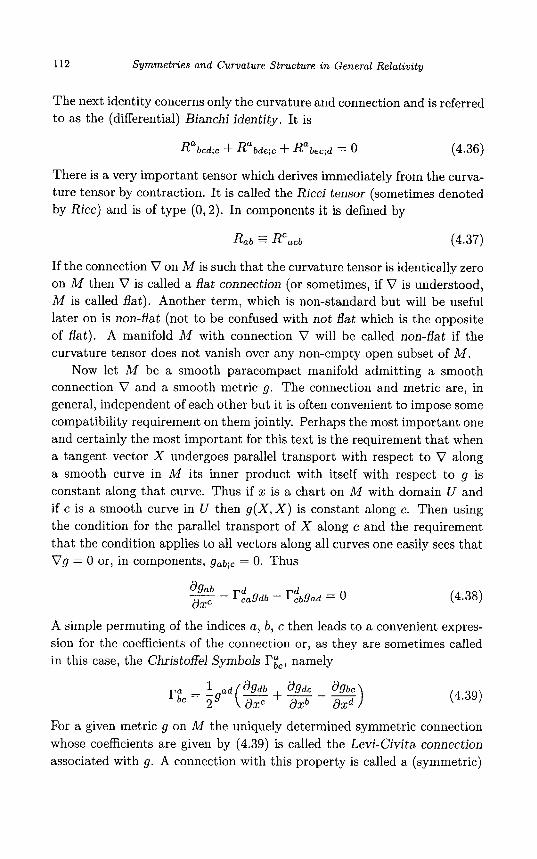
112 Symmetries and Curvature Structure an General Relativity
The next identity concerns only the curvature and connection and is referred to as the (differential) Bianchi identity. It is
Rabcd;e + Rabde;c + Rabec;d = O (4.36)
There is a very important tensor which derives immediately from the curva- ture tensor by contraction. It is called the Ricci tensor (sometimes denoted by Ricc) and is of type (0,2). In components it is defined by
R a b RCacb (4.37)
If the connection V on M is such that the curvature tensor is identically zero on M then V is called a flat connection (or sometimes, if V is understood, M is called flat). Another term, which is non-standard but will be useful later on is non-flat (not to be confused with not flat which is the opposite of flat). A manifold M with connection V will be called non-flat if the curvature tensor does not vanish over any non-empty open subset of M .
Now let M be a smooth paracompact manifold admitting a smooth connection V and a smooth metric g . The connection and metric are, in general, independent of each other but it is often convenient to impose some compatibility requirement on them jointly. Perhaps the most important one and certainly the most important for this text is the requirement that when a tangent vector X undergoes parallel transport with respect to V along a smooth curve in M its inner product with itself with respect to g is constant along that curve. Thus if x is a chart on M with domain U and if c is a smooth curve in U then g ( X , X ) is constant along c. Then using the condition for the parallel transport of X along c and the requirement that the condition applies to all vectors along all curves one easily sees that Vg = 0 or, in components, gab;c = 0. Thus
dgab - _ d X C
A simple permuting of the indices a, b, c then leads to a convenient expres- sion for the coefficients of the connection or, as they are sometimes called in this case, the Christoffel Symbols F t C , namely
(4.39)
For a given metric g on M the uniquely determined symmetric connection whose coefficients are given by (4.39) is called the Levi-Civita connection associated with g . A connection with this property is called a (symmetric)
Manifold Theory 113
metric connection and, in particular, a metric connection compatible with the metric g (and if V is flat, a metric compatible with V is called a flat metric). The compatibility condition Vg = 0 ensures that the inner product with respect to g of any two vectors parallely transported along any curve c is constant along c (and hence the constancy of the signature of a metric on a connected manifold stated in section 4.15). Also one can easily show that the object with components 6; (= 1 if a = b and zero otherwise) at m E M and in every coordinate system whose domain contains m is a (1,l) tensor at m. This then gives rise to an obvious tensor field 6 on M satisfying v b = 0, i.e. b;,, = 0. It then follows from the relation gabgbc = 6: that gabic = 0. HenLe the rules of raising and lowering indices commute with covariant differentiation in the sense that, for example,
T a b E T a c g c b * Tab;d = T a " ;&cb (4.40)
The curvature tensor of a connection naturally arose as a (1,3) tensor with components R a b c d . One can now define a global smooth type (0,4) tensor on M also denoted by R and also called the curvature tensor (or the Riemann tensor) and defined in components by
Rabcd = g a e R e b c d (4.41)
Then one has the extra algebraic symmetry relations
Rabcd = - R a b d c = - R b a c d , Rabcd = &dab (4.42)
These algebraic relations between the curvature components can then easily be used to show that the Ricci tensor defined in (4.37) is a symmetric type (0,2) tensor. Further, one can now define an important smooth real valued function on M denoted by R and called the Ricci scalar. In components it is given by
R = R a b g a b (4.43)
If n = dimM 2 3 and if in every coordinate system on M the curvature and metric tensor components satisfy
Rabcd = O ( 9 a c g b d - g a d g b c ) (4.44)
then the function Q is given by a = &, R a b = %gab and the Bianchi identity (4.36) forces cy to be constant (Schur's theorem - see, e.g. 1351). Such a manifold is said to have constant curvature Q. If (4.44) holds at some rn E M then M is said to be of constant curvature at m (a poor
114 Symmetries and Curvature Structure in General Relativity
notation it has to be admitted!). If n = 2 , (4.44) necessarily holds but a need not be constant.
With the notation of the previous paragraph if the Ricci and metric ten- sors are proportional so that, in coordinates, Rat, = Pgab for some function P, then P = a and M is called an Einstein space (and so if M has constant curvature it is an Einstein space). M is a proper Einstein space if P # 0. If n 2 3, suitable contractions of (4.36) show that R and hence 0 are con- stant. If M is flat it can be shown that each m E M admits a coordinate neighbourhood U in which the metric components gab are constant (and then a further coordinate transformation will ensure that the components gab take the appropriate Sylvester form everywhere in U ) .
Let g and g' be global smooth metrics on M . Suppose there exists a smooth function q5 : M + IR such that q5 is nowhere zero on M and such that g' = q5g. Then g and g' are said to be conformally related (or just conformal). If +(m) > 0 at each m E M then g and g' have the same signature at each m E M whereas if #(m) < 0 at each m E M the signature of g' is, in an obvious sense, the reverse of that of g at each m E M . There is an important (smooth) tensor that derives from the metric tensor on M but which is unchanged if it is recalculated using a conformally related metric. This is the Weyl tensor (or the conformal curvature tensor) which is denoted by C and defined in components (and only in the case that n = dim M 2 3) by
1 12-2 Cabcd = Rabcd - -(Racgbd + R b d 6 : - Rbc6; - Radgbc)-
(4.45)
The Weyl tensor (which is identically zero when n = 3) has some pleasant algebraic properties which can be calculated together here in terms of the components of the related type (Old) (Weyl) tensor Cabcd = gaeCebcd.
Cabcd = -Cbacd = -Cabdc = Ccdab (4.46)
(4.48)
However it is the Weyl tensor of type (1,3) given in (4.45) and not the type (0,4) version which has the conformally invariant property of being
Manifold Theory 115
the same for conformally related metrics. The converse is false in the sense that two metrics giving rise to the same Weyl tensor as in (4.45) are not necessarily conformally related. A counter-example will be given in chapter 9.
A smooth manifold A4 of dimension n>4 and admitting a smooth metric g is called conformally flat if its associated Weyl tensor vanishes identically on M . If this is the case then for each m E A4 there is an open neighbour- hood U of M , a flat metric h on U and a smooth function cr : U -+ R such that, on U , g = crh. Conversely if such neighbourhoods exist about each m E M the conformally invariant property of the Weyl tensor, together with the easily established fact that the Weyl tensor on a flat manifold vanishes identically, show that M is conformally flat. The manifold M is called non-conformally flat if the Weyl tensor does not vanish over some non-empty open subset of M (and the term not conformally fiat means the opposite of conformally flat). If dim M = 3 the Weyl tensor (4.45) vanishes identically on M whilst if dim M = 2 neighbourhoods like U above exist about each m E M. For such manifolds of dimension 3 there is another tensor which plays the role of the Weyl tensor in determining the existence of neighbourhoods such as U above. These results are discussed in [35].
Some other topics can be briefly dealt with here. Let X be a smooth covector field on the smooth Hausdorff manifold M . Then X is called exact (or a global gradient or normal) if there is a smooth function f : M -+ R such that X = df and X is called closed if, in any cordinate system on M , X,,b = Xb+. Clearly if X is exact it is closed and, if M is simply connected, X is closed if and only if it is exact [25]. For any manifold M , if X is closed then each m E M admits a connected coordinate neighbourhood U and a smooth function q5 : U + R such that X = dq5 (i.e. X, = 4,,) on U so that X is locally a gradient. The above terms are sometimes applied to a vector field X on a manifold M admitting a metric g if they apply to its associated covector field (section 4.15). There is a similar but more general condition on the covector field X (or its associated vector field where appropriate). Suppose each m E M admits an open connected neighbourhood U on which X = $d$ where $,$ : U -+ R are smooth. Then X is called hypersurface orthogonal. The name is unfortunate since no metric need be involved. It arises from the fact that if M admits a metric then on any open neighbourhood U on which d4 never vanishes the vector field associated with X is everywhere orthogonal to the submanifolds (hypersurfaces) of constant q5 in U (which exist from section 4.11, example (v)), that is, everywhere orthogonal to the vectors
116 Symmetries and Curvature Structure in General Relativity
tangent to these submanifolds. Thus this definition for a covector field X is a statement about X but for a vector field (when M has a metric g ) it is a statement about X and g . [For example, let X be a covector field on M such that X is nowhere zero on some coordinate neighbourhood U of M and is not hypersurface orthogonal on U . Let g be a metric on U and consider the vector field on U with components X " E gab&. Suppose U is chosen (as it can be) such that X a = 6: on U . Then for this vector field on U the associated covector field X , = gabXb is not hypersurface orthogonal (by definition) but, if h is the Euclidean metric on U , the covector field habXb = 6; is hypersurface orthogonal.] If a covector field X is hypersurface orthogonal and X ( m ) # 0 then, whilst not necessarily a gradient on some open neighbourhood of rn, it may be scaled so that it is. Of course a closed covector field is hypersurface orthogonal.
It is convenient here to mention a point of notation which involves the use of round and square brackets in coordinate expressions to represent complete symmetrisation and skew-symmetrisation, respectively. Thus, for example, if T a b and Tabc are tensor components at some point of a manifold then
As an example, if X is a nowhere zero covector field on M then the condi- tion for it to be hypersurface orthogonal is that in any coordinate system, x [ a , b x c ] = 0. This follows from the "form" version of the Frobenius (dis- tribution) theorem (see, e.g. 1221).
4.17 Grassmann and Stiefel Manifolds
Consider the vector space R" and let V R" be an rn-dimensional subspace of R". Suppose V is such that it may be spanned by rn vectors in R" which, in the standard basis for Rn, have components
(LO,. . . ,o , Z m + l , . . . ,xn),. . . , (0, . . * ,o , 1, Ym+l , . * * , Yn).
Then these vectors are uniquely determined by V and such m- dimensional subspaces may then be identified with the member (x,+l,. . . , x,, . . . , ym+l , . . . , yn) of This gives a one-to-one map from a subset of the set G(rn,R") of all rn-dimensional subspaces of R"
Manifold Theory 117
onto Rm(n-Pn). By extending this idea but choosing the 0's and 1's in slots other than the first m slots one obtains a set of m(n - m)-dimensional charts for G(m,R") which can be shown [19] to yield a smooth atlas for G(m,R"). The resulting manifold G(m,Rn) is then called a Grassmann manifold (in this case of all m-dimensional subspaces of R") and has di- mension m(n - m).
There is an alternative approach to the Grassmann manifolds which involves the introduction of a Stiefel manifold. An m-frame in R" is an ordered set w = (v1, . . . , vm) of m linearly independent vectors in R". Again with components in the usual basis for R" one can arrange the members of the m-frame w to get a bijective map from the set V(m,R") of m-frames in R" onto the set of n x m real matrices of rank m. An application of the ideas in section 3.11 shows that the latter set is an open submanifold of the mn-dimensional smooth manifold MnxmR. Hence the set V(m, R") becomes an mn-dimensional smooth manifold (with a global chart) called the Stiefel manifold of m-frames in R". If one then maps the frame w into the m-dimensional subspace of R" that its members span one obtains a map f from V(rn,Rn) onto G(m,Rn) which can be shown to be a submersion [19]. Defining the equivalence relation N on V(m,R") by z N y @ f(z) =
f (y ) one sees that G(m,R") is (diffeomorphic to) a quotient manifold of
Each Grassmann manifold is Hausdorff, second countable and compact (191. Also G(m,R") is connected as will be shown in section 5.7. The Grassmann manifold G(m,Rn) is diffeomorphic to G(n - m,Rn) as can be shown by employing the standard metric on R" (defined by (x,y) +
ziyi with x = (zl ,..., z") and y = (y', . . . , y") E R") and mapping a member V of G(m, R") into its orthogonal complement W with respect to this metric. The Grassmann manifold G(l , R"+l) is real projective space, usually denoted by P"R, and has dimension n.
V(m, R").

This page intentionally left blank
Chapter 5
Lie Groups
5.1 Topological Groups
Let G be a set. It has been seen in earlier chapters how G may be given the structure of a group with multiplication represented by . and how G may be given a topological structure 7. These structures need have no relationship to each other. But given that G has these structures one can arrange a compatibility requirement between them by insisting that for a , b E G, the group function $1 : G x G -+ G defined by & ( a , b) = a . b (or more simply ab) and the inverse operator $2 : G + G defined by q52(a) = a-l are continuous maps with respect to 7 and the corresponding product topology on G x G. If such is the case the set G together with its group and topological structure is called a topological group and will simply be labelled G given that . and 7 are understood. It is not difficult to see that for a given group structure on G there is always a topology on G (for example, the discrete topology) which makes it a topological group, but it is not necessarily unique. However, given a topology on a set G, the next paragraph shows that there may not exist a topological group structure for G (and if there does, it is not necessarily unique as the situation when a set is given two distinct group structures each with discrete topology shows). If GI and G:! are topological groups, a map f : G1 -+ G2 which is continuous and a group homomorphism is called a topological group homomorphism. If f is, in addition, a homeomorphism then it is called a topological group isomorphism and GI and Gz are isomorphic topological groups.
A subgroup H of a topological group G together with its subspace topol- ogy is itself a topological group and is called a topological subgroup of G. If H is an open (respectively closed) subset of G it is called an open (re- spectively closed) subgroup of G. If a E G the maps L a and Ra : G + G
119
120 Symmetries and Curvature Structure in General Relativity
given for g E G by L,(g) = ag and R,(g) = ga are called left and right translations. They are bijective and their inverses are also left and right translations respectively, i.e. L l l = La-l, R i l = R,-1. Although they are not necessarily (group) isomorphisms they are (topological) homeomor- phisms and, as a consequence, if H is an open subgroup of G, any right or left coset of H in G is an open subset of G. Hence if H is an open subgroup of G it is also a closed subgroup of G (since its complement is a union of such open cosets). The facts that La and R, are homeomorphisms show that not any topological space can be given a group structure to make it a topological group since a high degree of “topological homogeneity” is required.
The topological group G may be connected. If it is not, the component of G containing the identity el G,, and called the identity component, is particularly important. In fact G, is a normal closed subgroup of G (and the other components of G are the cosets of G, in GI there being no distinction between left and right cosets here since G, is normal - see section 2.2) [19].
The following result will be important later [19]. If G is a topological group then G, (which inherits the structure of a connected topological group) is such that it is generated by any open subset U in G, which contains e.
Any real vector space is a group and also a topological space (inherited through its manifold structure - see chapter 4). With these structures it is easily seen to be a topological group. Similarly, GL(n,R) is a topological group. More examples of topological groups can be found in the next section and in the standard texts (see, e.g. [36]). In particular, if G I , . . . , G, are topological groups then so is G1 x . . + x G, with its product group and topology structures.
It is remarked that for a set G with both a group and a topology struc- ture, the continuity of 41 does not imply the continuity of 4 2 , and vice versa (but the continuity of both is insisted upon in the definition of a topological group). In fact the family of subsets { [ a , b) : a, b E R} is a basis for a topol- ogy 7 on R such that, with respect to the usual additive group structure on R, $1 is continuous but 4 2 not. On the other hand the group G with three members { e l s l y } and identity e (+ zz = y, yy = z, zy = yz = e) and when given the topology 7 = {4, { e } , G} is such that 4 2 is continuous but 41 not. However, the continuity of the single map G x G -+ G given by ( a , b ) --f ab-l is equivalent to the topological group condition (just combine this latter map with the (continuous) map a -+ ( e , a ) to get the continuity of $2 and then with the (now continuous) map (a , b ) 4 (a , b-’) to see that
Lie Groups 121
$1 is continuous, the converse being clear).
5.2 Lie Groups
Let G be a group, Suppose that G can also be given the structure of a smooth manifold of dimension n. Again, these structures need not be re- lated. Suppose, however, that one insists on the compatibility requirement that the group function $1 : G x G + G is smooth when G x G is given the manifold product structure from G. Then G, together with its group and manifold structure, is called a Lie Group (of dimension n). It should be noted that it is not necessary to insist also that the inverse operator $2 : G + G is smooth. In fact it follows automatically for a Lie group that $2 is a (smooth) diffeomorphism on G [19]. Hence a Lie group with its given group structure and manifold topology is a topological group. The extra power in the manifold structure of a Lie group forces the smoothness of 4 2 from that of $1 whereas the continuity of both $1 and $2 must be assumed for a topological group.
Some elementary properties of Lie groups can now be briefly reviewed, further details being available elsewhere [19], [20], [22] (and, in fact, [I91 will be used as a general reference for much of this chapter). All topological references will always be to the underlying manifold topology. If G is a Lie group the left and right translations La and R, (a E G) and the inverse operator $2 are diffeomorphisms G + G. The identity component G, of G, where e is the identity of G, is an open (and closed) subset of G and hence an open submanifold of G. fiom the previous section G, is also a normal subgroup of G and its cosets in G are the (open and closed) components of G. These cosets are (smoothly) diffeomorphic to G,. Then G, inherits the structure of a connected Lie group which is generated by any open subset of G, containing e. Hence there are no open subgroups of G properly contained in G,. If GI, . . . , G, are Lie groups then GI x . . . x G, is a Lie group with the product group and manifold structures. It can be shown that if a topological group satisfies the TI property (section 3.8) then it is necessarily Hausdorff. However, the topology of any manifold is TI (theorem 4.3(ii)) and so every Lie group is Hausdorff. Also it can be shown that every connected Lie group is second countable (and, in particular, G, is second countable for any Lie group G). It follows that any connected Lie group is paracompact (theorem 4.4). With the obvious natural structures Rn, GL(n, C) and GL(n, R) are Lie groups. If GI and G2 are Lie groups
122 Symmetries and Curvature Structure in General Relativity
and f : G1 -+ Gz is smooth and a group homomorphism then f is called a Lie group homomorphism. If, in addition, f is bijective and f -’ is smooth it is called a Lie group isomorphism and GI and Gz are isomorphic as Lie groups (Lie isomorphic). It can be shown [22] that if f : GI -+ G2 is a topological group homomorphism then it is a Lie group homomorphism and hence that if G1 and Gz are isomorphic as topological groups they are isomorphic as Lie groups.
5.3 Lie Subgroups
A subgroup of a topological group G has a natural subspace topology and hence a natural structure as a topological subgroup of G. For a Lie group the situation is a little more complicated. Let G be a Lie group and H a subset of G. Suppose that H is both a subgroup of G and a submanifold of G and, that with these two structures, is itself a Lie group. Then H is called a Lie subgroup of G of dimension equal to that of H as a manifold. The complication is that the topology on H may not be subspace topology and in this sense H may not be a topological subgroup of G! It is, in fact, true that if G is a Lie group and H is a subset of G which is simultaneously a subgroup and a submanifold of G then H is a Lie subgroup of G. In other words the compatibility of these structures needed to give a Lie group structure on H follows automatically. This result is not obvious (see e.g. [22]) because the restriction of the group function $1 : H x H -+ H is not obviously a smooth map between the manifolds H x H and H (see e.g. theorem 4.7). It is obvious, of course, if H is a regular submanifold of G but this need not be the case. In what is to follow, and given that G is a Lie group and H C G, the statement that H is a subgroup of G means exactly what it says in the group theoretic sense whereas the statement H is a topological subgroup of G again means exactly what it says but with G regarded as a topological group. The statement that H is a Lie subgroup of G is as defined above.
A group usually becomes more interesting when it admits a manifold structure which then makes it a Lie group. Similar remarks apply when a subgroup of a Lie group is found to admit the structure of a Lie subgroup. In this respect, the following so called ‘closed subgroup theorem’ is important. A detailed discussion and proof can be found in [19].
Theorem 5.1 Let G be a Lie group and H a subgroup of G. If H is a closed subset of G which is not discrete then H admits a unique structure as

Lie Groups 123
a regular submanifold of G and is then a Lie subgroup of G. If, however, H is closed but not open then the set L(G, H ) of left cosets of H in G admits the structure of a Hausdorff quotient manifold of G.
Another useful result in this direction is
Theorem 5.2 Let G be a Lie group of dimension n and M a manifold of dimension m < n. Let f : G -+ M be a smooth map which has rank m at the identity e of G and let H = f -I{ f (e )} . Suppose also that f ( g h ) = f (9) for each h E H , g E G. Then H can be given the structure of a (closed) regular submanifold of G of dimension n - m and then the structure of a (closed) Lie subgroup of G of dimension n - m.
It is remarked that the “compatibility” of the structures on H between these theorems follows from section 4.11, example (viii). It is also remarked that it may be possible to give H in theorem 5.1 a non-regular manifold struc- ture so that it is then a Lie subgroup of G. As an application of these results consider the n2-dimensional Lie group GL(n, R). This group has two components: the identity component and its coset and which contain those non-singular matrices with positive determinant and negative deter- minant, respectively. Important subgroups of it are O(n) and SL(n, R). In fact the continuous maps f : GL(n,R) -+ S(n,R) and g : GL(n,R) -+ R given by f(A) = AAT and g(A) = detA show that they are the sub- sets f - l ( l n ) and g- ’ ( l ) , respectively, and are hence closed subgroups of GL(n,R). Since neither is discrete it follows from theorem 5.1 that each can be given a regular submanifold structure which then makes it a Lie subgroup of GL(n, R). The dimension of SL(n, R) is n2 - 1 and of O(n) is $n(n - 1) and this follows from theorem 5.2 by again employing the maps f and g . An application of these results to the Lorentz group will be given in section 6.3.
A Lie subgroup H of a Lie group G is called a connected Lie subgroup if H is connected in its manifold topology. It is then necessarily a connected subspace of G (but the obvious converse may fail and a counter-example can be constructed from the example following the proof of theorem 4.7). It can be shown that if a subset H of a Lie group G can be given two structures as a connected Lie subgroup of G then these structures are Lie isomorphic. Hence if, in addition, H is a closed subset of G this unique Lie subgroup structure on H makes H a regular submanifold of G from theorem 5.1. The Lie subgroup SL(n,R) is connected but O(n) is not. The latter has two components: the identity component denoted by SO(n) and its coset, consisting of those matrices with determinant +1 and -1, respectively. It
124 Symmetries and Curvature Structure in General Relativity
is noted here that, from the above and section 4.11, example (vii), O(n) and SO(n) are regular submanifolds of GL(n, R) and, clearly, the latter is an open submanifold of Rn2. Thus, since O(n) and SO(n) are bounded (and closed) subspaces of Rn2 they are compact (section 3.8).
5.4 Lie Algebras
There is an important vector space associated with a Lie group and which is called its Lie algebra. Before introducing this a few remarks on vector fields are required.
Let M be a smooth manifold and X a global smooth vector field on M and let f : M -+ M be a smooth diffeomorphism on M . The vector field X is called f-invariant if f+ o X = X o f (i.e. X is preserved when "pushed forward" by f* - see section 4.9). It is not hard to check that if X and Y are smooth vector fields on M which are f-invariant then so also is [ X , Y ] .
Now let G be a Lie group of dimension n with identity e and consider the left and right translations La and R, for each a E G, all of which are smooth diffeomorphisms of G. A global smooth vector field X on G is called left or right invariant if it is, respectively, La-invariant or Ra- invariant for each a E G. Now let v be a vector in the tangent space TeG to G at e and define a global vector field X on G by X ( a ) = L,,(v) for each a E G. Then it can be shown that X is a left-invariant vector field on G and that any left-invariant vector field X on G can be obtained in this manner from the vector X ( e ) E TeG. It is then clear that the set of left invariant vector fields on G is a real vector space isomorphic to TeG under the isomorphism X ( e ) -+ X and is hence of dimension n. (Thus any Lie group is parallelisable - see section 4.8.)
This vector space of left-invariant vector fields can be given the structure of a Lie algebra (see section 2.7) under the (Lie) bracket operation which associates with two such vector fields X and Y the global smooth vector field [ X , Y ] (since then [ X , Y ] is left-invariant). This Lie algebra structure is then transferred to TeG by the above isomorphism so that if u, v E TeG arise from left-invariant vector fields X and Y , respectively, on G (so that X ( e ) = u, Y ( e ) = v) then one defines [u,v] = [ X , Y ] ( e ) . If { v i } is a basis for TeG which arises, respectively, from left-invariant vector fields X I , . . . , X , on G it easily follows that [X,, xb] = cz=l czbXc where the czb E R are the structure constants in this basis. It follows that [v,, v b ] = cbl czbvc. The vector space T,G with this Lie algebra structure is referred
Lie Groups 125
to as the Lie algebra of G. It will be generically labelled LG although more specific symbols are available for the more commonly used Lie groups. It is remarked that analogous results hold for the right-invariant vector fields on G and the vector space T,G with its resulting Lie algebra structure is denoted by RG. The bracket operations in LG and RG are not the same but differ only in sign.
In order to see the role played by the Lie algebra of G consider the set of d-dimensional distributions on G (1 < d < n) which are left-invariant in the sense that they are preserved by all the left translations. More precisely a distribution D on G is left-invariant if for each a , g E GI D(ag) = L,,D(g). Clearly any such left-invariant distribution D uniquely determines a sub- space D(e) of T,G and conversely every subspace U of T,G uniquely de- termines a left invariant distribution D on G according to D(g) = L,,(U) Qg E G (and so D(e) = U ) . The question now arises as to the integrability of such left-invariant distributions and to the relations between left-invariant distributions in G, subalgebras of LG and Lie subgroups of G. To this and other ends, the following theorem is important.
Theorem 5.3 Let G be a Lie group with Lie algebra LG.
i) Let U be a subspace of T,G and D the associated left-invariant distri- bution on G (so that D(e) = U ) . Then D is integrable i f and only if U is a subalgebra of LG.
ii) Let H be a Lie subgroup of G with Lie algebra LH and let i : H --$
G be the (smooth) inclusion map. Then i,, : LH --f LG is a Lie algebra isomorphism between LH and a subalgebra of LG. Also H is an integral manifold of the left-invariant distribution on G determined by the subspace i,,(T,H).
iii) Let U be a subalgebra of LG. Then there exists a unique connected Lie subgroup H of G such that, if i is the inclusion map H --$ G, i,, is a Lie algebra isomorphism between LH and U .
Roughly speaking, theorem 5.3 says that each Lie subgroup of G picks out a unique Lie subalgebra of LG whereas each Lie subalgebra of LG is the Lie algebra of some (not necessarily unique) Lie subgroup of G and is the Lie algebra of a unique connected Lie subgroup of G. It should also be remarked that the Lie algebra U in part (iii) which was ultimately identified with the Lie algebra of a Lie group (i.e. the Lie algebra LH of H ) was assumed itself to arise as a subalgebra of the Lie algebra of a Lie group (ie. G). More generally one can show that any finite dimensional (real) Lie algebra is the

126 Symmetries and Curvature Structure in General Relativity
Lie algebra of a connected Lie subgroup of GL(n,R) for some n. This is a consequence of Ado's theorem (see e.g. [19]), It also follows that the Lie algebra of G is identical to that of G,.
As an example consider the Lie group GL(n,R). In section 4.11 it was shown that GL(n, R) is an open submanifold of MnR and since M,R admits a global chart so does GL(n,R). Let the n2 coordinate functions for this chart on GL(n,R) , in an obvious notation, be xab (1 < a , b, 6 n). The left-invariant vector fields on G can be obtained from the basis members (A), of T,GL(n,R) by employing the left translations in G. Thus one obtains left-invariant vector fields x a b defined at g (where g is the matrix gab) by x a b ( g ) = Lg, (A), and which take the general form x a b = PabCd (&) on G (recalling the summation convention). The functions P can be calculated for each choice of a and b according to
Hence Xab(g) = gca ( & ) g and in the above coordinates, x a b = xCa&. If one writes [Xab, Xed] = a p q & then
apq = Xab (Xcd(xPq)) - Xcd (Xab(xPq)) = Xab (xTChpprdqd) - Xcd ( X r a d p r d q b )
= (xPadqddcb - xpcdqbdad)
and so
[Xab, Xcd] = bcbxad - d a d x c b (5.1)
Now the Lie algebra of GL(n, R) must on grounds of dimension be isomor- phic (as a vector space) to M,R and so the product (5.1) may be transferred to MnR by means of the basis Eab for M,R, where Eab is the matrix with 1 in the ab position and zeros elsewhere, according to
[Eabr Ecd] = GcbEad - 6adEcb (5.2)
Thus if A = C Aij Eij and B = C Bij Eij are in M,R the Lie algebra binary operation can be found from 5.2 to be [A, B] = CAijB,,[Eij, Ern,] = AB - BA (the commutator of A and B).
Returning to theorem 5.2 it can be shown, in the notation of that the- orem, that the subalgebra of LG corresponding to the Lie subgroup H
Lie Groups 127
(identified with M ) is the subspace (f*)-' (0) where 0 is the zero vector of T f ( e ) M . Since the appropriate function f and manifold M are known (and were given earlier) for the Lie subgroups O(n) and SL(n, R) of GL(n, R) one can calculate their Lie algebras as subalgebras of the Lie algebra of GL(n, R) given above. For O(n) the map considered was f : GL(n,R) 4 S(n,R) given by f ( A ) = AAT which in the usual global charts xab for GL(n,R) and yab for S(n,R) (section 4.3, example (iv)) is yab o f = xacxbc. Now
So for a general member v = Bab (&), of TeGL(n,R) one has
Then the subalgebra of GL(n,R) associated with the Lie subgroup O(n) is (f*)-'(O), that is, the Lie algebra of O(n) is the vector space of skew- symmetric members of MnR (obtained by setting the expression in (5.3) equal to zero) under the binary operation induced by (5.2). A similar calculation for the Lie subgroup SL(n, R) using the determinant function shows that the Lie algebra of SL(n,R) is the vector space of tracefree matrices under the binary operation induced by (5.2).
5.5 One Parameter Subgroups and the Exponential Map
Let G be a Lie group with identity e and let X be a left-invariant vector field on G. Suppose c is an integral curve of X with domain some open interval I of Iw containing 0 and which starts at e (so that c(0) = e and C = X o c). For a E G consider the curve c, = La o c with domain I starting from a E G. Then with the usual coordinate t on the curve c

128 Symmetries and Curvature Structure an General Relativity
and SO C a is also an integral curve of X with the same domain I as c. Because there exists an integral curve of X with the same domain I through any point of G and since G is Hausdorff it can be shown that X is a complete vector field [19]. Hence each left-invariant vector field on G is complete.
This completeness feature turns out to be rather important for several reasons, the first of which can be described now. Let v E TeG, let X be the left-invariant vector field determined by v , so that X ( e ) = v, and let c be the maximal integral curve of X starting at e. One can then define a map called the exponential mapping for G, denoted by exp and defined as a map exp : TeG -+ G by expv = c(1). Sometimes one writes ev for expv. This map is defined on the whole of TeG (by the completeness described above) and is smooth when TeG has its standard manifold structure. Care must be taken not to confuse this exponential map with the exponential map arising from a connection (section 4.16). In fact, the exponential map described here can also be thought of as arising from a connection on G and its smoothness can be deduced from this fact. The name 'Lexponential" is suggested by the fact that if Q, P E R and v E TeG then
exp(a + P)v = exp QV exp Pv (5.4)
The real line R with its usual (identity global) chart and binary operation of addition is a l-dimensional Lie group. Let G be any Lie group and let f : R -+ G be a group homomorphism which is also a smooth map. Then f is called a l-parameter subgroup of G. It follows from (5.4) that for v E TeG the map $v : t -+ exp tv is a l-parameter subgroup of G. But one can say more. In fact, every l-parameter subgroup of G is of the form $v for some (unique) v E TeG. Now the range of $0 is {e} and, if v # 0, the range of 4" can be given the structure of a l-dimensional submanifold of G (because &, is an integral curve of the nowhere zero vector field g -i Ls*v on G - see section 4.13) and is also a subgroup. It follows from section 5.3 of this chapter that the range of $v is a l-dimensional Lie subgroup of G (and is often identified with the l-parameter subgroup above).
One of the important aspects of the exponential map is the way in which it generates members of G from the Lie algebra LG of G. Since GL(n, R) and certain of its subgroups play an important role in this book, this Lie group will be used now as an example of this feature. In the notation employed in the previous section and regarding GL(n,R) , and now denoting its Lie algebra by ge(n,R), let v = Vab (&), E g!(n,R) (V E MnR). The corresponding left-invariant vector field X on G is then
Lie Groups 129
X : g + Lg*v where
and so (replacing gab by xab)
Now an integral curve of this vector field is &, and so & = X o &. Now if cab = xab o $,,(t) = xab o exptv then from (5.6) one has
-- - vcbx""(f$v(t)) = vcbcac dcab dt
with initial condition ~ " ~ ( 0 ) = zab(e) = hab. The unique solution is
O0 tS cab = xab o exp tv = dab + C g ! ( ~ ~ ) ~ ~
s=l
where
O0 tS S!
exp tv = 1, + C -vS s=1
(5.7)
(5.8)
(5.9)
This notation is standard and no confusion should arise between it and the exp, notation of section 4.16.
A few remarks may be made here regarding the exponential map. First suppose H is a Lie subgroup of a Lie group G. Then one must distinguish between the exponential map associated with H (and denoted by expH) so that expH : TeH + H and the exponential map exp of G when restricted to T e H . Fortunately the relation between them is pleasant in the sense that if i : H -+ G is the natural inclusion map then expo i,, = i 0 expH. Thus the range of the curve $v : t -+ exptv for v E i,TeH lies in H . There is a converse result if H has a second countable topology (and note that from section (5.2) every connected Lie group is second countable) in that any smooth curve c in G whose range lies in H is such that every tangent vector k(t) is tangent to H . Second, one might ask whether the exponential map exp : T,G -+ G for a Lie group G is onto or not. If it is onto (that is every g E G equals exp(v) for some v E T,G) the Lie group is called exponential. Clearly, for a Lie group to be exponential it must be connected but this is not sufficient. Less obvious is the result that a connected Lie subgroup of an exponential Lie group need not be exponential. This feature will be
130 Symmetries and Curvature Stmcture an General Relativity
seen later when the Lorentz group is introduced. Clearly (the range of) any 1-parameter subgroup of a Lie group G is an exponential Lie subgroup of G. It can be shown that any compact connected Lie group is exponential [37] and that SL(2,R) is not. However every connected Lie group is "almost" exponential as the following theorem shows.
Theorem 5.4 Let G be a connected Lie group. Then every g E G is the product of finitely many members of G each of which is the exponential of some member of the Lie algebra of G.
Proof. This follows from the fact mentioned in section (5.2) that G is generated by any open subset of G containing the identity e of G. But the
O
It is convenient a t this point to mention briefly some properties of the exponential map. First consider the metric space Rn2 for some positive integer n with the usual Euclidean metric. The set M,R may be identified with this metric space and then one can talk sensibly about convergence of sequences of such matrices. If P E M,R then the series (5.9) for exp P can be shown to be convergent to a member of GL(n,R) and one has the following properties for B, P, Q E M,R and B non-singular.
range of exp is such an open subset and this completes the proof.
i) If Q = BPB-l then expQ = B(exp P)B- l . ii) If P Q = Q P thenexp(P+Q)=expPexpQ=expQexpP . iii) exp(-P) = (expP)-l. iv) If x is a (real or complex) eigenvector of P with (real or complex)
eigenvalue X then x is an eigenvector of exp P with eigenvalue ex. v) If P E M,R the map R t M,R given by t t etP is differentiable and
d -(exptP) = P e x p t P = (exptP) P. dt
vi) If 0 E M,R is the zero matrix, e x p o = I,. vii) If P E M,R and if v (0 # v E C") is an eigenvector of exptP with
eigenvalue X(t ) E C for each t E R then X ( t ) = ext (A E C ) and v is an eigenvector of P with eigenvalue A.
The proofs of (i)-(vi) can be found in [38],[22]. For (vii) one has v exp tP =
X(t)v and so X( t ) is a smooth function on R. Also setting t = 0 gives X(0) = 1 and, since exptP is non-singular, X( t ) # 0, V t E R. Now differentiate and use (v) above to get (vexptP) P = i v or VP = h - ' v where = 2. So is constant and it follows that X( t ) = ext (A E C) and hence that V P = Xv.
Lie Groups 131
5.6 Transformation Groups
Let G be a group and M a smooth manifold. Then G is said to act on M as a transformation group if there is a map q5 : G x M + M with the properties that
i) given g E G the function q5g : M 4 M given by q5g(m) = q5(g,m) is a
ii) if g, h E G, q5g 0 q5h = q5gh.
smooth diffeomorphism of M ,
If e is the identity of G then the map q5e is necessarily the identity map on M . This follows because if m E M and m’ = +;‘(m) then &(m) = $e(q5e(m’)) = q5e(m’) = m. However e may not be the only member of G which gives rise in this way to the identity map on M . If e is the only such member of G, G is said to act effectively (or to be an effective action) on M . If +e is the only such map to fix any point of M then G is said to act freely (or to be a free action) on M . Clearly a free action is effective. Now let g E G. Then 9g- l = e and so q5g o q5g-i = &. It follows that 4;’ = q5g-1. Since each (Pg is a diffeomorphism it follows that the map q5 : G x M -+ M is surjective. The action of G on M is said to be transitive if given ml,ma E M 3 9 E G such that q5g(ml) = m2.
The above action q5 : G x M -+ M is, for obvious reasons, sometimes referred to as a left action and G is said to act (on M ) on the left. A right action of G on M can be defined as a map 11, : M x G + M such that (i)’ for g E G, the map ll,g : m + ll,(mlg) is a diffeomorphism of M and (ii)’ for g , h E G, qg o 11,h = $hg. It should be pointed out that there is nothing special about G and M that produces a left action rather than a right action, or vice versa, because if q5 is a left action of G on M then the map 11, : M x G -, M given by $(m,g) = $ ( g - I , m ) is a right action, and vice versa. However, unless otherwise specified, a transformation group action will always refer to a left action as defined above
5.7 Lie Transformation Groups
Let G be a Lie group and M a smooth manifold. Then G is said to act on M as a Lie transformation group if there is a smooth map q5 : G x M ---f M satisfying the conditions (i) and (ii) given in the previous section. [Note that (ii) may be rewritten as $(g,+(h,m)) = q5(gh,m) for each m E M and g,h E G.] Thus G acts on M as a transformation group and the
132 Symmetries and Curvature Stmcture in General Relativity
notation of the previous section will be employed here. However, for a Lie transformation group the conditions (i) and (ii) can be replaced by an equivalent set (i)" and (ii) where (i)" is the condition that the map 4 is surjective (see, e.g. [19]). Clearly (i) and (ii) imply (i)" and (ii). For the converse one notes that if m E M then, from (i)", there exists m' E M and h E G such that (Ph(m') = m and SO 4e(m) = $e(&(m')) = &(m') = m and so 4e is still the identity map on M . It is then immediate that for g E G, 4, has an inverse function +,-I and that the smoothness of 4, follows from that of 4. Hence each 4, is a diffeomorphism of M . The terms effectively and freely will be used with the same meaning as in the previous section. Also the remarks about left and right actions in the previous section apply also to Lie transformation groups and although the results to follow are stated for left actions they apply equally well for right actions when appropriately rewritten.
In the following examples of Lie transformation groups (i), (iv) and (v) are right actions, (ii) and (iii) are left actions and (vi) is either.
i) 4 : R" x GL(n, R) 4 R" where 4(v, A) = vA. ii) q5 : GL(n,R) x S(n,R) + S(n,R) where 4(A, S) = ASAT. iii) 4 : GL(n, R) x M,R 4 M,R where 4(A, B ) = ABA-'. iv) 4 : R" x O(n) 4 R" where 4(v,A) = vA. v) 4 : S"-l x O(n) -+ S"-l where +(v,A) = vA.
vi) Let X be a complete vector field on a smooth Hausdorff manifold M (section 4.10). Then the map 4 : R x M + M given by @(r,m) = c,(r) = $T(m) where c , is the maximal integral curve of X starting at m, is smooth and satisfies the condition that 4r 0 $s = q5T+s (r, s E R). This shows that the Lie group R acts on M as a Lie transformation group.
It is remarked that modifications of examples (ii) and (iii) to (S ,A) -+
ATSA and ( B , A) -+ A-lBA produces right rather than left actions. The action represented by example (iii) is not effective whereas (i) and (iv) are effective but not free.
Let G act on M as a Lie transformation group as described above. If H is a Lie subgroup of G then, by restricting the map 4 above to a map H x M 4 M , one sees that H also acts on M as a Lie transformation group (see examples (i) and (iv) above). Also, a subset A of M is invariant under G if q5(G x A) C_ A. An equivalence relation - on M is said to be preserved by G if for m1,mz E M and g E G, ml - mz + r$,(ml) N d,(mz). One can now show that if N is a regular submanifold of M which is invariant
Lie Groups 133
under G then G acts (in an obvious way) as a Lie transformation group on N . (The problem here for a general submanifold N of M is the smoothness of the resulting map G x N -+ N (see section 4.11). This problem is avoided if N is regular.)
Theorem 5.5 Let G be a Lie group acting as a Lie transformation group on the smooth manifold M and let N be an equivalence relation on M which leads to a quotient manifold M I N of M and which is preserved by G. Then G acts naturally on M / N as a Lie transformation group.
This theorem has the following consequence. Suppose that H is a subgroup of G and L(G, H ) the set of left cosets of H in G. Suppose also that L(G,H) can be given the structure of a quotient manifold of G. Then the group function $1 : G x G 4 G shows that G acts on itself as a Lie transformation group and clearly leads to a well defined map G x L(G, H ) -+
L(G, H ) . So by the previous theorem G acts on L(G, H ) on the left as a Lie transformation group with action (9, a H ) -+ (ga )H. The same results hold with left everywhere replaced by right. Another consequence is that the action of GL(n,R) in example (i) above leads to an obvious action on the Stiefel manifold V(m, Rn) and hence on the Grassmann manifold G(m, Rn) which is a quotient manifold of V(m,Rn) (see section 4.17). Restricting this action to the identity component of GL(n,R) and to a single member of G(m,Rn) and noting that the range of this restricted action is connected and equal to G(m,R") shows that G(m,Rn) is connected.
5.8 Orbits and Isotropy Groups
Let a Lie group G act on a smooth Hausdorff manifold M as a Lie trans- formation group. The Hausdorff assumption will be needed later in this section and is imposed now as a blanket statement for the whole section. Define an equivalence relation N on M by ml N m2 if there exists g E G such that $,(ml) = m2 (m1,mz E M ) . The associated equivalence class containing m E M is {$,(m) : g E G } and is denoted by 0, and called the orbit of m (under G). If for m E M one defines the map $m : G --+ M by $,(g) = q5(g,m) then $, is smooth and its range is the orbit 0, of m. If the action of G on M is transitive there is only one orbit, which is M . If G is connected it follows that each orbit is a connected subset of M .
Again for m E M consider the subset of G whose members g "fix" m. This set is {g E G : $,(m) = m} and is easily seen to be a subgroup of
134 Symmetries and Curvature Structure in General Relativity
G. It is also equal to the set 4h1{m} and is denoted by I , and called the isotropy group at m (under G). If ml and m2 are members of the same orbit (so that there exists g E G such that $,(ml) = m2) then if g' E I,, it follows that 4;' o 4,) o $,(rnl) = ml and so g-lg 'g E I,,. A similar argument in reverse then shows that I,, and I,, are conjugate (and hence isomorphic) subgroups of G.
The isotropy group I , at m is a subgroup of G and leads to the set L(G, I,) of left cosets of I , in G. If 91, g2 are in the same left coset then it follows that $,(g1) = $,(gZ) and so 4, gives rise to a map 4, :
L(G, I,) 4 M given by $,(gI,) = $,(m) and whose range is the orbit 0, of m. Also if glIm and 921, are members of L(G, I,) then the condition $rn(glIm) = $m(g2Im) implies that 4g1(m) = $g2(m). Thus 4,;lg,(m) =
m and so 91'92 E I,. Hence 911, = 921, and so $, is one-to-one. Now I , = 4;' {m} and so since M is TI it follows that I , is a closed subgroup of G. Thus either I , is an open subset of G or L(G, I,) admits the structure of a quotient manifold of G and either I , is discrete or it admits a unique structure as a regular submanifold of G and is then a Lie subgroup of G (theorem 5.1). If ml and m2 lie on the same orbit, then Iml and I,, are either both discrete or diffeomorphic. One now has the following theorem.
Theorem 5.6 Let G be a Lie group which acts as a Lie transformation group on the smooth Hausdorff manifold M . Then for m E M one has the following results.
a) If I , is not open in G the map $, : L(G, I,) 4 M is a smooth one- to-one immersion whose range is 0,. Hence the orbit Om of m can be given the structure of a Hausdorff submanifold of M diffeomorphic to L(G, I,) under the map $,. If I , is discrete, dim 0, = dim G and if not, dim 0, = dim G - dim I,.
i i) If G is second countable and acts transitively on M then L(G, I,) (which cannot now be discrete) is diffeomorphic to M . If also the action is free then G and M are diffeomorphic.
It should be noted in conjunction with part (ii) that any connected Lie group (e.g. the identity component of any Lie group) is second countable.
Under the conditions of part (i) of the above theorem the orbit 0, has a submanifold structure and the original action 4 : G x M + M induces an obvious action 4' : G x 0, -+ 0, on 0,. This would immediately be smooth if Om were a regular submanifold of M . Although 0, need not be a regular submanifold of M the smoothness of 4' can still be established as
Lie Groups 135
the next theorem shows.
Theorem 5.7 Let G be a Lie group which acts as a Lie transformation group on the smooth Hausdorff manifold M . Let m E M and suppose I , is not open in G. Then G acts on 0, as a Lie transformation group.
Proof. Let 4‘ be the restriction G x 0, 4 0, of the original action of G on M . Clearly 4’ is surjective. The previous theorem guarantees that the map $Im regarded as a map $Jm : L(G, I,) 4 0, is a diffeomorphism. One can also define a diffeomorphism 1-1 : G x L(G, I,) - G x 0, by the map ( 9 , q ) -+ (9 , $Jm(q)) and a smooth map v : G x L(G, Im) -+ L(G, I,) by the map (g,gII,) 4 ggII, (see end of last section). The proof is completed
0
It is remarked that for m E M , if I , is not an open subgroup of G (so that L(G,Im) is a quotient manifold of G), then if X : G + L(G,I,) is the natural submersion one has 4, = $Im o X with $Im now regarded as a smooth map L(G, I,) -, 0, and so 4, can be regarded as a smooth map from G onto 0,. Hence if G is connected, 0, is a connected submanifold of M . It is also pointed out that if M is paracompact (as will usually be the case in this book) and G connected then 0, is connected, paracompact and second countable. This follows by noting that the component MO of M containing 0, is closed and hence paracompact (section 3.8) and so admits a global smooth positive definite metric. This metric induces a similar one on 0, and so 0, is paracompact and second countable (theorem 4.14).
As an application of theorem 5.6 consider the left action (example (ii) section 5.7) of GL(4, W) on S(4, R) given by $(A, S) = ASAT and let SO = diag(-1,111) E S(4,R). Then Iso is the Lorentz group and, since not discrete, it is a Lie subgroup of GL(4,R) of dimension six (see chapter 6) and so is not an open submanifold of GL(4,R). The corresponding orbit Oso is then, by theorem 5.6, a submanifold of S(4,R) diffeomorphic to L(GL(4,R),Is0) and dimOs, = dimGL(4,R) - dimIs, = 16 - 6 = 10. Since dim S(4, W) = 10, Oso is an open submanifold of S(4, R). Similar results apply if SO is changed to diag(lll1) (and then Iso is the orthogonal
by noting that 4’ = $Im o v o p - l .
group O(4)).
5.9 Complete Vector Fields
Return now to the Lie group G with identity e and let X be a left-invariant vector field on G with X ( e ) = v E T,G. It was mentioned earlier that the
136 Symmetries and Curvature Structure in General Relativity
integral curve of X starting at e is the curve 4,, : t -+ exptv. For any other a E G it was shown at the beginning of section 5.5 that the integral curve of X starting at a is the curve t -+ L,(exp tv). So the integral curves of X are obtained by left translations from the curve 4". If Y is a right- invariant vector field on G satisfying Y ( e ) = u E TeG the integral curve of Y starting at e can also be shown to be the curve & : t -+ exp tu and an argument similar to that for left-invariant vector fields shows that for a E G the integral curve of Y starting at a is the curve t -+ R,(exptu). Thus the integral curves of Y are obtained by right translating the curve q5u. Let H,, be the subgroup of G defined by the range of 4,,. Then if X and Y are left- and right-invariant vector fields, respectively, on G satisfying X ( e ) = Y ( e ) = v E TeG the ranges of their integral curves in G are, respectively, the left and right cosets of H,, in G.
The right-invariant vector fields on G can be mirrored in M by an important family of vector fields on M . Let v E TeG and m E M . One can define a vector in TmM using v and the map 4, : G -+ M , & ( g ) = $ ( g , m ) , namely the vector &,v. The collection of all such vectors, one at each m E M , determined by v can be shown to give rise to a smooth vector field X on M . The set of all such vector fields obtained in this way from each v E TeG is then a real vector space of smooth vector fields on M , denoted by R(G, M ) (for reasons that will become clear later) and the map f : v + 2 is a linear map from TeG onto R(G, M ) . Hence R(G, M ) is finite-dimensional with dimension 5 dim G. Further, if I , is not open in G and since 4, can be regarded as a smooth map G 4 Om, it follows from the definition of 2 and theorem 7.7(iii) that each member of R(G, M ) is tangent to 0,. It can also be shown 1191 that the rank of qj*m equals the dimension of 0, and hence that each orbit is an integral manifold of the distribution on M arising from R(G, M ) . Now let X be the right-invariant vector field on G determined by v E TeG, so that X ( e ) = v. Then for a E G and m E M
Now let g E G and put $,(a) = m'. Then
4m 0 % ( g ) = 4rn(ga) = 4(ga ,m) = 4 ( g > 4 ( a , m ) ) = 4 r n / ( g ) (5.11) -
It follows that $,,X(a) = = X ( m ' ) and so the right-invariant vector field X on G arising from v E T,G is related to the vector field 2 on M arising from v in a natural way with respect to the map q5m for any m E M .
Lie Groups 137
It should be noted here how the original left action of G on M represented by the map q5 here leads naturally to consideration of right-invariant vector fields on G. Continuing, let X1 and X2 be right-invariant vector fields on G and XI and X 2 the corresponding vector fields on M related to X1 and X2
under the map q5*m for each m E M . It can then be shown that [ X l , z z ] is similarly related to [XI, X,]. Evaluating this relation at e then shows that R(G, M) is a (finite dimensional) Lie algebra of smooth vector fields on M under the bracket operation and that the map f above is a linear map between the Lie algebras RG and R(G, M) which preserves the algebra structures, i.e. [ f (vl) , f(v2)] = f [Vl ,V2]R for v1,vz E RG and where [ ]R denotes the algebra operation in RG. The notation R(G, M) is now clear.
Let 2 = f (v) be the vector field on M arising from v E RG as described above. The relation between the right-invariant vector field X on G arising from v, and X, under the map q5m for m E M shows that the map t --f
g5m(exptv) = q5exptv(m) is an integral curve of X starting from m and defined on R. This together with the arbitrariness of m shows that X is a complete vector field on M .
Theorem 5.8 If the Lie group G acts on a smooth Hausdorff manifold M as a Lie transformation group then R(G, M) is a finite-dimensional (in fact of dimension < dim G) Lie algebra of smooth complete vector fields on M . If the action of G on M is effective R(G, M) is Lie isomorphic to RG under f .
Proof. Only the last sentence has not been established. So suppose v E RG and f (v) is the zero vector field on M . Consideration of the integral curves discussed above now shows that q5exptv(m) = m, Vm E M and V t E R. The effective assumption then shows that exptv = e, V t E R and so v = 0. Thus f is one-to-one and hence bijective.
The above results help to give an elegant geometrical interpretation of the action of G on M. For example the action of the members of the subgroup H , = {exptv : t E R} of G on m E M simply traces out the integral curve starting at m of the vector field X on M associated with v E T,G. Also for g E G, m E M let K = q5m(H,g) be the image in M under q5m of the right coset Hvg of H, in G. Then
K = { h g ( m ) : h E Hv) = {&(&(m)) : h E Hv)
and so K (which is the range of the integral curve of x starting from 4 m ( g ) ) can be thought of either as the set of all images of m under the action of
138 Symmetries and Curvature Structure in General Relativity
all members of H,g or as the set of all images of q5g(m) under the action of all members of H,. Theorem (5.4) has the following interpretation.
Theorem 5.9 Let G be a connected Lie group which acts on a smooth Hausdorff manifold M as a Lie transfonnation group. Then for any g E G there exists a positive integer k such that the associated map $g : M + M can be described by
4g(m) = q5expvl(q5expvz(...$expvk(m) . * * ) )
for members v1, v2,. . . , vk of TeG.
Proof. The proof follows from theorem 5.4 by writing g = 9192.. . gk 0
The interpretation is that the map q5g can be regarded in k stages each of which has the form +expv for some v E TeG and which moves the appro- priate point a parameter distance unity along the integral curve starting at that point of the member of R(G, M ) associated with v under f .
Thus the action of G as a Lie transformation group on a smooth Haus- dorff manifold M leads to a finite-dimensional Lie algebra of smooth, com- plete vector fields R(G, M ) on M . These vector fields facilitate a geometri- cal interpretation of the action of G on M . One naturally asks the question whether such a Lie algebra of vector fields on M necessarily gives rise in this way to a Lie group acting as a Lie transformation group on M . The answer is provided by the beautiful theorem of Palais [39].
Theorem 5.10 Let S be a non-trivial finite-dimensional Lie algebra of smooth complete vector fields on a Hausdorfl manifold M . Then there is a connected Lie group G which acts effectively on M as a Lie transformation group and is such that the Lie algebra R(G, M ) associated with this action equals S .
where g1 = exp v1, g2 = exp v2, . . . , gk = exp vk.
5.10 Groups of Transformations
So far the discussion has concerned an abstract action of a Lie group G on a manifold M described by a function q5 : G x M + M . This action then gives rise to a diffeomorphism q5g : M + M for each g E G. Suppose, however, one is not given this action of a Lie group G on M but rather a set G of diffeomorphisms of M which form a group under the usual rules of composition, identity and inversion of such maps. Can one find a Lie group
Lie Groups 139
structure for G such that the map G x M -+ M given by (g,m) + g(m) is smooth? This, from section (5.7), would mean that G now acts on M as a Lie transformation group. However there may be more than one such action and an extra condition is needed to guarantee uniqueness (see, e.g.
Suppose then that G is a group of diffeomorphisms of a Hausdorff man- ifold M under composition, identity and inversion, as described above. If X is a smooth complete vector field on M such that each of its associated diffeomorphisms $r : M + M (section (5.7) example (vi)) belongs to G then X is said to be tangent to G. Such a group G is called a Lie group of transformations of M if it admits a Lie group structure such that
[W
i) the map $ : G x M t M given by $(g,m) = g(m) is smooth, ii) for any smooth complete vector field X on M which is tangent to G the
map R -+ G given by r + 4,. is a smooth group homomorphism (i.e. a one-parameter subgroup of G).
The following theorem now summarises the situation [39] where the distinction between a Lie group of transformations and a Lie transformation group should be noted.
Theorem 5.11 A group G of diffeomorphisms of a Hausdorff manifold M admits a t most one structure as a Lie group of transformations of M . The map $ then shows that, given such a structure, G acts on M as a Lie transformation group and the action is effective. G admits the structure of a Lie group of transformations of M if and only if the set S of smooth complete vector fields on M which are tangent to G is a finite-dimensional Lie algebra under the bracket operation. If such is the case then G acts effectively on M as a Lie transformation group and S = R(G, M ) (in the notation of section (5.9)).
A curious fact emerges in the proof of this result [39]. If X and Y are smooth complete vector fields on a Hausdorff manifold M then neither X + Y nor [X,Y] need be complete. Hence if S is the Lie algebra of all smooth vector fields on M and S’ is a subset of complete members of S, the smallest subalgebra S” of S which contains S’ (the subalgebra of S generated by S’) need not consist only of complete vector fields. However, if S’’ is finite-dimensional, every member of S” is complete.
140 Symmetries and Curvature Structure in General Relativity
5.11 Local Group Actions
In the last five sections the transformations on M which have been discussed have been diffeomorphisms of M . Often one is led, directly or indirectly, to transformations which are only defined on part of M and to this situation attention can now be turned.
Consider a smooth vector field X on a smooth Hausdorff manifold M . Then given m E M there exists E > 0 and an open subset U of M containing m such that for any p E U an integral curve cp of X exists which is defined on ( - E , E ) and starts at p (theorem 4.6). This gives rise, for each t E ( - E , E ) ,
to a map q5t : U + $ t ( U ) defined by p --t c p ( t ) for each p E U . So each point of U is moved a parameter distance t along the integral curve of X through that point. Each map q5t is smooth and is, in fact, a diffeomorphism between the open submanifolds U and q5t(U) of M . However, for t # 0, q5t may not be defined on the whole of M and is so defined if and only if there exists an integral curve of X defined on the same open interval of R starting at any point of M . This is equivalent to X being complete [19] and then every such map $t constructed above is a diffeomorphism of M . Thus whereas smooth complete vector fields on M lead to an action of R on M as a Lie transformation group (section (5.7) example (vi)), incomplete smooth vector fields on M lead to “local diffeomorphisms” of M . This leads to the idea of a flow box associated with X [21],(22].
Theorem 5.12 Let X be a smooth vector field on a Hausdorff manifold M . For each m E M there exists a triple (U,~ ,q5) , called a flow box of X at m, where
i ) U is an open submanifold of M containing m, E E R and E > 0 or
i i) q5 : (-el E ) x U --t M is smooth, iii) for each p E U the map cp : ( - E , E ) + M given by c p ( t ) = q5(tlp) is an
integral curve of X starting from p , iv) if t E ( - E , E ) the map q5t : U 4 q5t(U) defined by $ t ( p ) = $ ( t , p ) is a
smooth diffeomorphism between the open submanifolds U and q5t(U) of M .
E = 00,
Such a flow box is unique in the sense that if (U’, E’, 4’) is another triple satisfying (i)-(iv) above then q5 and 4’ agree on the intersection of their domains. Also, if s, t and s + t E ( - E , E ) then q5s o q5t = q5t 0 q5s = q5s+t
wherever these compositions are defined and $0 is the identity map on U .
Lie Groups 141
Finally if Ut = 4 t ( U ) and if U nu, # 0, 4t and 4-t restrict to inverse maps between Ut n U and U-t n U .
If X is complete 4 is a smooth map R x M + M and is referred to as the Aow of X and the set {qbt : t E R} as a I-parameter group of diffeomorphisms. If X is not complete each map q5tl t E ( - - E , E ) , is called a local diffeomorphism or a local Aow (associated with X). [It is remarked here for occasional use later that if the vector field X is Ck ( l c 2 1) the associated local flows rbt are Ck local diffeomorphisms.]
The way in which a flow box handles the case when X is not complete suggests the following formal definition of a local group action due to Palais [39]. Let G be a connected Lie group with identity e and M a smooth Hausdorff manifold. A local G-transformation group acting on M is a smooth map 4 : D -+ M where
i) D is an open subset of G x M such that for each p E M the subset D, = { g E G : ( g , p ) E D } of G is a connected open neighbourhood of e.
ii) for each p E M , $ ( e , p ) = p . iii) if ( h , p ) E D , (g ,qh(h ,p) ) E D and ( g h , p ) E D then 4 ( g h , p ) =
4(9, 4(hl P I ) .
It should first be noted that if D = G x M then G acts on M as a Lie transformation group and the discussion of (5.7) applies. The local nature of the action is expressed in the facts that for p E M only members of D, “act” on p and a particular g E G may only “act” on the open subset D, = { p E M : ( g , p ) E D } of M and which it does so through the smooth
An infinitesimal G- transformation group acting on M is a Lie algebra preserving linear map from RG to the Lie algebra of smooth vector fields on M . The link between local and infinitesimal G-transformation groups is provided by another the- orem due to Palais but a further definition is required before this can be done. Returning to the local G-transformation group action on M , define a smooth map 4, : D, -+ M by & ( g ) = 4 ( g , p ) and a linear map f from RG to the Lie algebra of smooth vector fields on M which associates with v E T,G the vector field given by p -+ &*v. This vector field is smooth and the map f, called the infinitesimal generator of 4, is Lie algebra preserving 1391.
map 4 g : D, + M given by 4 , ( P ) = 4(9 , P ) . Let G be a connected Lie group as above.
Theorem 5.13 If G is a connected Lie group and 4 a local G-
142 Symmetries and Curvature Structure in General Relativity
transformation group acting o n a Hausdorff manifold M then the associated infinitesimal generator f is a n infinitesimal G-transformation group acting o n M (and necessarily & * X ( g ) = f ( X ( e ) ) # ( g , p l f o r each right-invariant vector field X o n G and ( g , p ) E D). Conversely every infinitesimal G - transformation group acting on M is the infinitesimal generator of some local G-transformation group acting on M
Since any finite-dimensional Lie algebra is the Lie algebra of some Lie group (Ado’s theorem - see section 5.4) the general thrust of this theorem is that finite-dimensional subalgebras of the Lie algebra of global smooth vector fields on M arise as the result of local G-transformation group actions on M for various connected Lie groups G, and vice-versa (whereas the global actions (section (5.9)) arise as a result of finite-dimensional Lie algebras of global complete vector fields on M and vice-versa). As an example let M be a Hausdorff manifold and X a smooth vector field on M . Then, from theorem 5.13, X gives rise to a local R-transformation group on A4 (cf. theorem 5.12) and, if X is complete, to a Lie transformation group on M (G = IR in theorem 5.10) from section 5.7 example (vi).
In studying symmetry in general relativity one is, perhaps, tempted to appeal (in a not very precise way) to a certain family of local diffeo- morphisms on the space-time M satisfying the particular symmetry under consideration. Even with a precise definition of such a family it may be rather difficult to work with in practice. In later chapters of this book when such symmetries are considered, a lead will be taken from this sec- tion by assuming them to arise as the local flows (again with the appropriate symmetry requirement) of a certain family S of global smooth vector fields on M . These local flows (symmetries) satisfy any reasonable requirement of such a symmetry and the “generating” vector fields in S are easier to work with. Usually (but not always - see chapter 13) S turns out to be a finite-dimensional Lie algebra of vector fields under the bracket operation and such Lie algebras are considered in the next section.
5.12 Lie Algebras of Vector Fields
This section is, in a sense, a completion of the work of section 4.13 and, in particular, of theorem 4.13. Let S be a non-trivial real Lie algebra of smooth vector fields on a smooth connected paracompact manifold M . The binary operation on S is the usual Lie bracket of vector fields and, as before, S, = { X ( r n ) : X E S } C T,M. Each X E S gives rise to a family
Lie Groups 143
4t of local diffeomorphisms of M for appropriate t and S gives rise to a generalised distribution m ---f S, of the type introduced in section 4.13.
Let k be a positive integer, let X I , . . . , xk E s and let 4:, . . . ,4: be the local diffeomorphisms associated with X I , . . . , Xk respectively. The local group G of local diffeomorphisms of M generated by S is the set of all maps (where they are defined)
(5.12)
for all choices of k, X I , . . . , X k and ( t l , . . . , t k ) E Rk under the usual formal rules of composition and inverses. The right hand side of (5.12) is defined in an open neighbourhood of m and for ( t l , . . . , t k ) in some open neigh- bourhood of the origin in Itk. (The actual algebraic properties of G need not concern us here and the term “local group” will be taken to mean that which is described here and nothing more-see [30]).
The sets S and G lead to a structure on M which can now be discussed. Define an equivalence relation - on M by ml - m2 if and only if there exists a E G such that a(m1) = m2. The resulting equivalence classes are the orbits in M of (associated with) G (or S ) and, from theorem 5.9, coincide (where applicable) to those defined in section 5.8. It would obviously be convenient if the orbits could be given some structure within M and if they could be related to the map m ---f S,. This is provided by the following extension of theorem 4.13 due to Hermann [28], Sussmann [30] and Stefan k l .
Theorem 5.14 let S be a non-trivial Lie algebra of global smooth vector fields on M .
i ) Each orbit of S can be given the structure of a smooth leaf of M . ii) If S is locally finitely generated, then there exists a unique maximal
integral manifold of S through each m E M and each orbit 0‘ of S is a maximal integral manifold of S with dimof = dims, for any m E Of and is also a leaf of M . Fhrther, S i s invariant in the sense that for each m E M and f E G, f3, G Sf(,,,).
Let M be a smooth connected paracompact manifold and
Again it is remarked for completeness that the conditions and conclusions of (ii) hold in the particular case when S is finitedimensional. The orbits of S are not necessarily regular submanifolds of M . The relationship between the work of this section and that of sections 5.7-5.9, when the members of S are complete vector fields, is clear. It is noted that an alternative proof of theorem 5.7 is now available, in the case when G is connected, from

144 Symmetries and Curvature Structure an General Relativity
theorems 5.9 and 5.14 and the discussion in section 4.11 since the orbits are then leaves of M .
5.13 The Lie Derivative
Let M be a smooth Hausdorff manifold and let T and X be a global smooth tensor field and a global smooth vector field on M , respectively. Let & for appropriate t represent the local diffeomorphisms associated with X . A measure of the change in T along the integral curves of X in the vicinity of m E M can be obtained as a kind of Newton quotient involving the differences between T(m) and the pullbacks $,*T evaluated at m and the parameter t . This leads to a type of derivative of T along X called the Lie Derivative. It is a global smooth tensor field on M of the same type as T , denoted by C x T and defined by
1 t-+O t C x T ( m ) = lim-[(q!(T)(m) - T(m)]
First it should be noted that this limit always exists [22]. The Lie derivative has the following properties, where f , Y and S are any global smooth real valued function, vector field and tensor field on M , respectively, and a , b E R [20],[21],[22]. Here, smooth functions M -+ IR are regarded as (0,O) tensors.
i) ii)
iii) iv)
vi) v)
The operator CX is always R-linear and commutes with all contractions. C x f = X ( f ) . C X Y = [ X , Y ] . L x ( S @ T ) = C x S @ T -k S @ C x T . Cax+byT = aCxT + bCyT. C [ X , Y I T = C X ( C Y T ) - C Y ( C X T ) .
If in some coordinate domain T and X have components T,?: and X a , respectively, then the tensor C x T has components given by
The left hand side of (5.13) will usually be written (with a traditional abuse of notation) as CXTZ::;~”. It is useful to note that if M admits a symmet- ric connection then the right hand side of (5.13) is unchanged if partial
Lie Groups 145
derivatives are replaced by covariant ones (i.e. the commas are replaced by semi-colons) .
The following results relating the Lie derivative and the maps 4: will be important in what is to follow (see e.g. [20],[40])
vii) q5:T = T for all dt * C X T = 0. viii) q5:T = eatT for all q5t and some fixed a 6 R * LxT = aT.
ix) 4:T = eX(t)T for all q& and where x is a smooth real-valued function with appropriate domain and possibly dependent on the flow of X from which the maps r$t arise % CxT = $T for some smooth real-valued function $J with appropriate domain.
It will be useful here to collect together some miscellaneous results re- garding the members of the Lie algebra S of all global smooth vector fields on M . First let X E S with associated local diffeomorphisms q5t and let 4 : M -+ M be a smooth diffeomorphism on M . Then the pushforward & X E S and its local diffeomorphisms are of the form 4 o q!Jt o 4-l. If Y E S with associated local diffeomorphisms $Jt then [ X , Y ] E S and its local diffeomorphisms are of the form $Jt' 04t10$toq5t and from this result and those immediately above it one can show that the following statements are equivalent (where (iv), (v) and (vi) below are assumed to hold for all appropriate s and t ) [21].
(5.14)
In particular the commuting condition (vi) between the local diffeomor- phisms associated with X and Y is equivalent to the vanishing of [ X , Y ] . Finally, if M I and MZ are manifolds, 4 : M I -+ M2 a (smooth) map, X a vector field on M I , Y a vector field on MZ with $+X = Y and T a type (0, s) tensor field on M2 then [21]
(i) C X Y = 0 (iv) $t+Y = Y (v) + t J = X (vi) 4t 0 $, = $Js 0 dt
(ii) C y X = O (iii) [ X , Y ] = O
4*(CYT) = Cx(+*T). (5.15)

This page intentionally left blank
Chapter 6
The Lorentz Group
6.1 Minkowski Space
In this section a brief description of Minkowski space will be given. This space can be presented in two different ways each based on the set W4. First one may regard W4 as a 4-dimensional real vector space together with the Lorentz inner product r] and defined by r](u,v) = r]abUaVb where u, v are members of W4 with components ua and va , respectively, and r]ab is the matrix diag(-1, 1, 1,l). In this form it will simply be referred to as Minkowski space. Second, one could regard W4 as a Cdimensional smooth manifold admitting the global smooth Lorentz metric r] whose components in the natural global chart on R4 are r]ab. In this form it will be referred to as Minkowski space-time because it is thus that it is usually used in special relativity. There is a very natural link between them obtained by noting that the tangent space at any point p of Minkowski space-time is just Minkowski space when taken with the inner product r ] (p) . Then the completeness of the Levi-Civita connection associated with r] may be used to show that the exponential map at any point of Minkowski space-time provides a smooth diffeomorphism between it and Minkowski space (with its natural manifold structure as a vector space). This identification will always be assumed made.
A non-zero member v of Minkowski space is called, respectively, space- like, timelike or null according as r ] ( ~ , v) is positive, negative or zero. Let S, T and N denote, respectively, the subsets of EX4 consisting of all the spacelike, timelike and null members. Then one has a disjoint decomposi- tion (classification) of Minkowski space in the form W4 = S U T U N U (0) where 0 is the zero vector of W4. A 1-dimensional subspace (henceforth called a 1-space or a direction) of Minkowski space is then called, respec-
147
148 Symmetries and Curvature Structure in General Relativity
tively, spacelike, timelike or null if it is spanned by a spacelike, timelike or null vector. The collections of such subspaces are labelled in an obvious notation by S1 , 7'1 and N I , and this classifies all 1-dimensional subspaces of Minkowski space.
A vector v in Minkowski space is called a unit vector if [q(v,v)I = 1. A basis {e ,} of Minkowski space consisting of four mutually orthogonal unit vectors is called an orthonormal basis (or tetrad) and necessarily one member is timelike and the others spacelike. A basis {fa} of Minkowski space is called a (real) null basis (or tetrad) if the only non-vanishing inner products between them are q(f3 , f3) = q ( f 4 , f d ) = q ( f 1 , f i ) = 1 (so that f1
and f2 are null and f3 and f4 unit spacelike). Now consider the set of all 2-dimensional subspaces of Minkowski space
(henceforth called 2-spaces). This set may be disjointly decomposed in the form 5'2 U TZ U NZ where the members of SZ (called spacelike 2-spaces) contain no null vectors, where the null vectors in any member of N 2 (called a null 2-space) are confined to a single null direction and where the null vectors in any member of T2 (called a timelike 2-space are confined to two distinct null directions. That this classification is exhaustive follows quickly by assuming a certain 2-space contains three distinct null 1-spaces and obtaining a contradiction from the fact that if u and v are orthogonal null vectors then u = Xv for some X E R. It easily follows that all non- zero vectors in any member of 5'2 are spacelike and that any member of T 2
contains spacelike, timelike and null members. If V E N Z then V contains a unique null direction, called the principal null direction of V , and all other members of V are spacelike and orthogonal to (any non-zero member of) this null direction. The two null directions in a member of Tz are also referred to as its principal null directions. A spanning pair of vectors for any 2-space V may always be chosen orthogonal but if they are, and V is null, one of them must span the principal null direction and if V is timelike one must be spacelike and one timelike. The orthogonal complement of a spacelike 2-space is timelike and vice-versa (here the fact that the only vectors orthogonal to a given timelike vector are spacelike is used) and in this case a spanning pair from each 2-space together give a basis for Minkowski space. The orthogonal complement of a null 2-space V is also null and V and its orthogonal complement V' have the same principal null direction. In this case V and V' intersect in exactly their common principal null direction.
Now consider the set of all 3-dimensional subspaces (3-spaces) of Minkowski space. Such a 3-space is called, respectively, spacelike, time-
The Lorentz Group 149
like or null if its orthogonal complement is a timelike, spacelike or a null 1-space. Alternatively one can characterise such 3-spaces as spacelike if they have no null members, null if their null members are confined to a single null direction (again called its principal null direction) and timelike if they contain two (and hence infinitely many) null directions. The collec- tions of such types of subspaces are labelled in an obvious notation by S3, T3 and N3 and their union exhausts all possible 3-spaces. Spanning sets for a spacelike (or timelike) 3-space and its orthogonal complement together give a basis for Minkowski space but the same is not true for a null 3-space V because then V’- coincides with the principal null direction of V and is hence contained in it. If V E SJ, all non-zero members of V are spacelike whereas if V E T3, V contains timelike, spacelike and null members. If V E N3 then all members of V are either in its principal null direction or else orthogonal to any member of this null direction and spacelike. One may always choose a spanning set of mutually orthogonal vectors for any 3-space V but if V is timelike one of these vectors must be timelike and the others spacelike and if V is null one of them must span its principal null direction.
It is convenient at this point to introduce the idea of a wave surface [41]. Let 1 be a null vector in Minkowski space. A wave surface to 1 is a spacelike 2-space each member of which is orthogonal to 1. The set of all wave surfaces to 1 is denoted by W(l) and clearly W(l) S2. Also a consideration of orthogonal complements shows that any member of S2 is a wave surface for the non-zero members of exactly two null 1-spaces.
Clearly S and T are open submanifolds of R4. The subset N is nei- ther open nor closed in R4 and can be given the structure of a regular 3-dimensional submanifold of R4 (section 4.11, example (zJ)). The subset N U (0) is closed in R4 and is the (topological) boundary of both S and T . The subset S is connected but T and N are not and this latter remark leads to the concept of ‘future and past pointing’ and will be discussed in section 6.2. The set N has two components and a consideration of the smooth maps S2 x R+ + R4 given by (x,t) + t (x , f l ) , whose combined ranges is the regular submanifold N of R4 , shows that each component is diffeomorphic to S2 x Rs. The topological and manifold theoretic properties of the sets S,, T,, N, (n = 1,2,3) and W(l) will be discussed in section 6.3.
150 S y m m e t r i e s and Curvature Strzlcture in General Relat iv i ty
6.2 The Lorentz Group
Minkowski space has associated with it an important group of linear trans- formations which preserve its inner product structure.
Let C be the set of all linear maps f : R4 -+ R4 satisfying
r](f(X), f (Y)) = r](x, Y) vx,y E R4 (6.1)
Thus C is the set of all linear maps R4-+R4 which preserve the inner product r]. It follows from (6.1) that
r](f(x), f(x)) = r](x, x) vx E EX4 (6.2)
and so, obviously, f preserves the 'size' associated with r] . The condition (6.2) appears at first sight to be weaker than (6.1) but is, in fact, equivalent to it as a consequence of the linearity of the members of C. To see this let f:R4 --+ R4 be linear, let z, y E R4 and suppose that f satisfies (6.2). Then r](f(x+y),f(x+y)) = r](x+y,x+y) and on expanding this out one easily achieves (6.1). The set C forms a group under the usual composition, in- version and identity operations. These are easily checked except, of course, one must show that each f E L is bijective and hence has an inverse. So let f E C and y E R4 and suppose that f(y) = 0. Then for any x E R4
d x , Y) = r](f(X), f(Y)) = 0 (6.3)
So r](x,y) = 0 Vx E R4 and since r] is non-degenerate, one finds y = 0. It follows that f is injective and, since it is linear, it is also surjective and hence a bijection R4 -+ R4. The corresponding inverse transformation f-' is also a member of C because it is linear and because
Vx, y E R4. The set C with the binary operation of composition is thus a group called the Lorentz group and its members are called Lorentz transfor- mations. Each member of L is an isomorphism of R4 and can be represented by a non-singular 4 x 4 real matrix. First choose the standard basis {e,} of R4 as orthonormal with respect to r ] , that is, r ] ( e a , e b ) = r]ab. Suppose f E C is represented with respect to this basis by the matrix A = ( a a b ) so that (recalling the summation convention) f ( e a ) = Uabeb . Then if x, y E R4 with x = xaea and y = yaea one finds f (x) = a a b x a e b and f (y) = a a b Y a e b
and (6.1) is equivalent to
abaxbacdYc%d = xbYcr]bc vx , Y E R4 (6.5)
The Lorentz Group 151
This is equivalent to the matrix relation
AqAT = q. (6.6)
So for a fked orthonormal basis the transformations in C are characterised by their representative matrix A satisfying (6.6). The subgroup of members A of GL(4,R) satisfying (6.6) is then isomorphic to the Lorentz group C according to the map which associates with f E C the matrix A (and if g E C is represented by the matrix B then go f is represented by AB - but see the remark at the end of section 2.2). If a different basis ( 6 , ) is chosen for R4 with 6 , = Ctabeb (T = ( t a b ) E GL(4, R)) and h,b = q(Qa, 6 b ) then if the above f E C has matrix A with respect to the basis (6 , ) then (6.1) is equivalent to
AhAT = h
and A and A are related by A = TAT-l. These equations describe the Lorentz group in a different basis to the
standard basis of R4. It can be regarded as a different representation of C (ie. an isomorphic copy of C) within GL(4,R) under the isomorphism A + A determined by T.
Minkowski space has been viewed here as a real (Lorentz) inner prod- uct space. It is sometimes convenient to extend the inner product q to the complex vector space C4. If z, w E C4 have components z, and w,, re- spectively, in the usual basis for C4 define q(z, w) = r]abZaWb. This will be considered as a formal device for dealing with situations where the complex field unavoidably arises (such as in the next theorem). The terms null and orthogonal will still be used for complex vectors in an obvious way, using 7.
The following theorem collects together some algebraic information about C. In it, the term invariant 2-space will always refer to a r ed 2- space (i.e. a subspace of R4). The usual (fixed) basis is chosen for R4 (and hence C4). A Lorentz transformation is then identified with its matrix, and a vector with its components, in this basis. In compiling this theorem the papers [42]-[44] were useful.
Theorem 6.1
i) A E C + detA = z t l ii) A E C + A ~ E C
iii) If a E C is an eigenvalue of A E C then af0 and a-' is an eigenvalue of A-' and also of AT and A.
152 Symmetries and Curvature Structure an General Relativity
iv) If a E C is an eigenvalue of A E C with a corresponding non-null eigenvector then la1 = 1. The result is false if the non-null condition is dropped.
v ) I f r and s are eigenvectors of A E C with eigenvalues a and p, respec- tively, then either q(r, s ) = 0 or p = a-'.
vi) If a E C\R is an eigenvalue of A E C then la[ = 1 and the corresponding complex eigenvector is null with its real and imaginary parts orthogonal and spacelike and spanning a spacelike invariant 2-space of A.
via) A (E C ) always admits an orthogonal pair of invariant 2-spaces. A timelike invariant 2-space of A always contains two distinct real eigendi- rections. If A admits a spacelike invariant 2-space then either it con- tains two distinct real eigendirections or else A admits two (conjugate) complex null eigendirections whose real and imaginary parts span this 2- space. A null invariant 2-space of A always contains a real null eigendi- rection and possibly another (necessarily real spacelike) eigendirection. Iff admits no non-null invariant 2-spaces then all its invariant 2-spaces are null with the same principal null direction and (from part (ui)) all its eigenvalues are real.
Proof. Part (i) is clear from (6.6). To prove (ii) take the inverse of each side of (6.6) to see that (A-l)T E C and hence, by the group property, that AT E C. The first statement in (iii) is true for all non-singular ma- trices. The next part follows because if x E C4 is an eigenvector of A with eigenvalue a E C then xA = ax and multiplying on the right by A-l gives xA-' = a-'x and so x is an eigenvector of A-' with eigenvalue a-'. Next, multiplying (6.6) on the left by x gives (xq)AT = a-'(xq) and so xq is an eigenvector of AT with eigenvalue a-'. That a-' is an eigenvalue of A follows because any matrix is similar to its transpose. To establish the first part of (iv) one has (using the notation of the proof of (iii)) q(xA,xA) = q(x ,x ) and on expanding this one finds q(x,x) = a2q(x,x) and the result follows. A counter example for the second part will be seen later. For ( v ) one has rA = ar and sA = p s and so q(rA, sA) = apq(r, s ) . This leads to q(r , s ) = apq(r,s) and the result follows. To establish (vi) let x be an eigenvector of A with eigenvalue a E @\R. Then one has xA = ax, XA = hx and, as in the previous two proofs, q(x, x ) = a2q(x, x) and q(x, f) = la12q(x, x). If x is not null then the first of these gives a' = 1 and the contradiction that a E R. So x is null. If, in addition, q(x,X) = 0 then writing x in terms of its real and imaginary parts, x = a + ib for a, b E R4, one finds that q(a, a) = q(b, b) = q(al b) = 0 and so x is a
The Lorentr Group 153
(complex) multiple of a real null vector. This again implies that a E R. Thus q(x,%) # 0 and hence = 1. For the final part of (vi) one has a null eigenvector x = a+ib as above and so q(x, x) = 0 a q(a, a) = q(b, b) and q(a, b) = 0. Also the fact that the corresponding eigenvalue a E C\R means that neither a nor b is null. It follows that they are spacelike (and orthogonal). Finally, writing a = y + i6 (7, 6 E R), the real and imagi- nary parts of the equation (a + ib)A = (y + iS)(a + ib) show that a and b span an invariant 2-space of A (which the previous sentence shows is spacelike). To prove (vii) one notes that an invariant 2-space always exists (section 2.6) and that its orthogonal complement is also invariant follows from the definition of the Lorentz group. So let U be an invariant timelike 2-space. Then U contains exactly two null 1-spaces spanned say by 1 and n which are chosen such that ~ ( 1 , n) = 1. By the definition of the Lorentz group either these 1-spaces are the required eigendirections or 1 A = An, nA = A - l l (0 # A E R). In this case 1 f An are real, non-null, orthogonal eigenvectors of A contained in U (with eigenvalues f l ) . If U is a spacelike invariant 2-space the restriction of a Lorentz transformation to U is a lin- ear orthogonal transformation on a copy of 2-dimensional Euclidean space and the result follows. If U is a null invariant 2-space the definition of a Lorentz transformation and the uniqueness of the principal null direction of U shows that this latter null direction is a real null eigendirection of A. Later it will be seen that other (necessarily spacelike) eigendirections may, but need not, exist in U . Finally if f admits null invariant 2-spaces with distinct principal null directions any two of these latter directions give rise to an invariant timelike 2-space. This contradiction completes the proof.0
Let a, b and c be, respectively, a timelike, a spacelike and a null vector in Minkowski space. Then it is straightforward to show that there exist f1 , fi and f 3 E C such that fl(a) = (p,O,O,O), fi(b) = (O,O,O,v) and f 3 ( c ) = (1,0,0,1) for appropriate positive real numbers p and v. By using this result it is easy to show that if V is any of the sets s k , Tk or Nk (k = 1,2,3) or the set of all wave surfaces or the set of orthonormal bases or the set of all null vectors and if f E C then, in an obvious notation, f ( V ) = V . Further C is transitive on V in the sense that if x,y E V there exists f E C such that f(x) = y. The same is also true for the set of all timelike or spacelike vectors v of a fixed “size” q(v, v).
There is a decomposition of the Lorentz group which can now be de- scribed. Consider the set T of all timelike vectors in Minkowski space. Then it is easily shown by considering continuous curves in the open submanifold
154 Symmetries and Curvature Structure in General Relativity
T of R4 that T has two path components and hence two components TI and T” and that in some (any) orthonormal frame these components are distinguished by the sign of the first component of the member of T . Now define, with the obvious topologies, a continuous map f : T x T + R\{O} by f (u,v) = q(u,v). Clearly f takes positive and negative values. Now T x T has four components and it follows since v E T + q(v,v) < 0 and since v E TI + -v E T” (and vice versa) that f maps the connected sub- sets T‘ x T‘ and T” x T“ to the negative reals and the connected subsets TI x T“ and TI’ x TI to the positive reals. Thus the relation N on T defined for u, v E T by u N v @ q(u, v) < 0 is an equivalence relation on T with two equivalence classes TI and TI’. A similar argument then shows that the set N of null vectors in Minkowski space also has two components and a continuity argument shows that it satisfies the condition that these compo- nents may be labelled N’ and N“ in such a way that k E N’ (respectively k E NI’) ej q(k, u) < 0 Vu E TI (respectively V u E TI’). Then the set C of all timelike and null vectors may be partitioned as C = C1 U C2 where Cl = T’ U N’ and C2 = T” U N”. The members of one of these subsets, say C1, are called future pointing and those of the other past pointing.
Now let f E L. From the previous paragraph it is clear that f maps each of the partitions C1 and C2 onto itself or maps each one onto the other. In the former case f is called future preserving and in the latter case, future reversing. The future preserving members of C form a subgroup of L but the future reversing members do not. Now return to theorem 6.1 noting that each A E L (in the usual representation) satisfies det A = f l , the sign being independent of the orthonormal base chosen. Those with det A = 1 also form a subgroup of L whilst those with det A = -1 do not. The group L can now be decomposed into four disjoint subsets L = L i UC: UL: UL! where the superscripts and 1 refer, respectively, to future preserving and future reversing and the subscripts + and - to the sign of the determinant. In this decomposition only L i is a subgroup of L and it is particularly important. It is described by various adjectives in the literature (“proper”, “orthochronous”) and will be given the symbol LO here. Its significance will become more apparent later when C is considered as a Lie group. The subgroup LO turns out to be a normal subgroup of L and C i , L: and L! are the cosets of LO in L which, in the matrix representation, can be obtained from LO by multiplying on the left (or right), respectively, by the
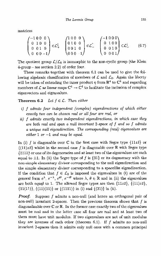
The Lorentz Group 155
matrices
- 1 0 0 0 1 0 0 0 - 1 0 0 0
( 0 0 0 1 l o 0 (;;; ; ) € d (; (6.7)
0 0 0 - 1 0 0 0 - 1 0 0 0 1
The quotient group C/Lo is isomorphic to the non-cyclic group (the Klein 4-group - see section 2.2) of order four.
These remarks together with theorem 6.1 can be used to give the fol- lowing algebraic classification of members of C and LO. Again the liberty will be taken of extending the inner product 77 from IR4 to C4 and regarding members of C as linear maps C4 -+ C4 to facilitate the inclusion of complex eigenvectors and eigenvalues.
Theorem 6.2 Let f E C . Then either
i ) f admits four independent (complex) eigendirections of which either exactly two can be chosen real or all four are real, or
i i) f admits exactly two independent eigendirections, in which case they are both real and span a null invariant 2-space off and so f admits a unique null eigendirection. The corresponding (real) eigenvalues are either 1 or -1 and may be equal.
In (i) f is diagonable over C in the first case with Segre type {IlzZ} or {(ll)zZ} whilst in the second case f is diagonable over R with Segre type { 11 11) or one of its degeneracies and at least two of the eigenvalues are each equal to fl. In (ii) the Segre type of f is (31) or its degeneracy with the non-simple elementary divisor corresponding to the null eigendirection and the simple elementary divisor corresponding to a spacelike eigendirection. If the condition that f E LO is imposed the eigenvalues in (i) are of the general form e A , e-Al eisl e-ie where A, 0 E IR and in (ii) the eigenvalues are both equcl to 1. The allowed Segre types are then { l l ~ z } ~ {(ll)zZ}, {11(11)}, {(11)(11)} or ((1111)) in (i) and ((31)) in (ii).
Proof. Suppose f admits a non-null (and hence an orthogonal pair of non-null) invariant 2-spaces. Then the previous theorem shows that f is diagonalisable over C or R. In the former case exactly two of the eigenvalues must be real and in the latter case all four are real and at least two of them must have unit modulus. If two eigenvalues are not of unit modulus they are inverses of each other (theorem 6.1). If f admits no non-null invariant 2-spaces then it admits only null ones with a common principal
156 Symmetries and Curvature Stmcture in General Relativity
null direction (spanned, say, by 1 which is then an eigendirection of f ) and all its eigenvalues are real (theorem 6.1). It is clear that f is not diagonalisable (over R) because it would then necessarily admit a non- null invariant 2-space spanned by an appropriate pair of eigenvectors. If f admits three independent (real) eigenvectors (one of which may be taken as 1) then a non-null invariant 2-space of f necessarily results and hence a contradiction. If f admits a single eigendirection (necessarily spanned by 1) then its Segre type is (4). But then f admits (at least) an orthogonal pair of null invariant 2-spaces spanned say by 1 and x and by 1 and y with x and y unit orthogonal spacelike vectors each orthogonal to 1. The properties of C together with part (iii) of the previous theorem show that one then has
where €1, €2 and €3 = f l and b, d are non-zero real numbers. Two possi- bilities arise: either €1 differs from at least one of €2 and €3 or €1 = €2 = €3.
In the former case suppose, say, that €1 = -62. Then € 1 ~ - ibl is an eigenvector o f f (with eigenvalue -61) contradicting the uniqueness of the eigendirection spanned by 1. In the latter case, €1 = €2 = €3 = E say, and one sees that dx - b y is an eigenvector of f with eigenvalue E and again a contradiction is achieved. The conclusion is that f admits exactly two (nec- essarily real) eigendirections and hence that its Segre type is either (31) or (22). But the Jordan matrix associated with type (22) easily reveals two invariant 2-spaces of f which intersect only in the zero vector and so this type is impossible since, now, no non-null invariant 2-spaces of f exist. Hence the Segre type is (31) or its degeneracy and by theorem 6.1 (iii) and (iv) (since now there exists a non-null eigenvector) the eigenvalues may only be f l . If these two eigenvalues are distinct one can take the eigenvectors as a null vector 1 and a unit spacelike vector x which are orthogonal and have eigenvalues +1 and -1 (or vice versa). By extending 1 and x to a null tetrad a calculation shows that either an extra (forbidden) eigenvector arises in the null 2-space orthogonal to that spanned by 1 and x or else the determinant of the matrix representing f is -1. Hence if f E LO the Segre type is { (31)) and the corresponding eigenvalue is unity since f is future preserving. A consideration of the Jordan canonical form for the matrix representing f together with the fact that all invariant 2-spaces of f are null and contain 1 then shows that 1 corresponds to the non-simple elementary divisor and x to the simple one. 0
The above possibilities for f E LO (f # identity) can be conveniently (and
The Lorentz Group 157
conventionally) represented as follows (cf. [42]) by piecing together the re- sults of the previous two theorems.
f (1) = e x l f(n) = e-’n (0 # x E R) (6.8a)
f (XI = x
f(m) = ei’m f(e) = e-i’ m - ( 0 < 0 < 2 . / r )
f(Y) = Y
f(1) = 1 f(n) = n (6.8b)
f(1) = e x l f(n) = e-’n (0 # x E R) (6 .8~) f(m) = e‘Qm f(e) = e-i’ m - (0 < 0 < 2 . / r )
1 2
f(n) = n - yy - -y21 (0 # y E R) (6.8d) f (1) = 1
f (4 = x f(y)=y+yl
In these equations (1, n, x, y) is an appropriate null tetrad with 1 and n null vectors and the complex null vector m is given by J2m = x + iy (so that q(m, m) = 1). In (6.8a) the Segre type is {11(11)) with eigenvectors 1, n, x, y and corresponding eigenvalues ex, e-’, 1,l. In (6.8b) the Segre type is ((1l)zZ) with eigenvectors 1, n, m and m and corresponding eigenvalues 1, 1, ei’, ePis (0 < 8 < 27r) except when 8 = T when the Segre type is ((11)(11)). In (6 .8~) the Segre type is {IlzZ} with eigenvectors 1 , n, m, m and corresponding eigenvalues ex, e-’, e iQ, e-iQ except when 8 = T
when the Segre type is (ll(11)). In (6.8d) the Segre type is ((31)) with eigenvectors 1 and x and corresponding eigenvalues each equal to 1 and y E R, y # 0. The null invariant 2-spaces spanned by the pairs 1,y and 1, x contain one independent eigenvector and two independent eigenvectors, respectively. The identity member of LO has Segre type ((1111)). The transformations (6.8a) are called boosts (in the In plane) whilst those in (6.8b) are called (spatial) rotations (in the xy plane) with angle 8. A transformation of type (6 .8~) is called a screw motion whilst one of type (6.8d) is called a null rotation (about 1).
From the above results one can see that every (non-identity) member of Co “fixes” at least one and at most two real null directions (ie. admits at least one and at most two real null eigendirections). Both these results are false if LO is replaced by C (simply consider the transformations f (1) = n, f(n) = 1, f (m) = m and f(1) = 1, f (n) = n, f(x) = x, f(y) = -y where in each case f E L\Co). Also i f f E Lo (f # identity) admits an orthogonal pair of invariant non-null2-spaces then this pair is unique. Again this result
158 Symmetries and Curvature Structure in General Relativity
is false if Lo is replaced by L (as the second of the above examples shows). Note also that the member f E C\Co given by
1 2 f (1) = -1 f(n) = -n + -d21 + dy (6.8e)
f (4 = x f(Y) = -Y - dl
where d E R, d # 0, has Segre type (31) with eigenvalues f l . Finally the null rotation (6.8d) can, by changing to the real null tetrad (l’, n’, x’, y’) where 1’ = yl, n’ = y-ln, x’ = x, y’ = y, be written in the simple form ( cf. [421)
f(n’) = n’ - y’ - -1 1 ’ 2
f (1’) = 1’
f(x’) = x’ f (y’) = y’ + 1’ (6.8f)
6.3 The Lorentz Group as a Lie Group
In this section L will be regarded as the subgroup of GL(4, R) whose mem- bers A satisfy (6.6). Now GL(4,R) is a Lie group of dimension 16 (section 5.2) and the map g : GL(4, R) --$ M4R given by A -t AqAT - q is a smooth map such that g-l{O} = L where 0 is the zero matrix in M4R. Hence L is a closed subgroup of GL(4,R) and, since it is not discrete, it follows from theorem 5.1 that L can be given a unique structure as a regular submanifold of GL(4, R) and is then a Lie subgroup of GL(4, R).
There is another construction which gives more detail about 13, in par- ticular, its dimension and its Lie algebra. Let S(4 ,R) denote the set of symmetric 4 x 4 real matrices with its standard 10-dimensional manifold structure (section 4.3) and let $J be the smooth map $J : GL(4, R) -+ S(4, R) given by A -t AqA*. If x and y are the standard charts on GL(4,R) and s ( 4 , R) with coordinate functions x a b and Y a b , respectively, then Y a b o $ J = Xacr)cdXbd. Now compute where e is the identity of GL(4,R), by computing its action on a general member of TeGL(4, R) represented by
The Lorentz Group 159
From this result two important conclusions follow. Firstly, it is easy to check from the final step in (6.9) that $,e is surjective and hence has rank 10 (= dim S(4,R)). Also it follows from the definition of $ that $-‘($(e)) = C and that if A E GL(4,R) and A E C then +(AA) = $(A). Hence from theorem 5.2 it follows once again that C can be given the structure of a Lie subgroup of GL(4, R) with an underlying regular submanifold structure. h r t h e r , the dimension of C equals dimGL(4,R) - dimS(4,R) = 6. The uniqueness remark at the end of the previous paragraph shows that the Lie group structures for C obtained here and in that paragraph are the same (cfsection 4.11 example (viii)) and this structure is then the conventional 6- dimensional Lie group structure for C. Secondly, it also follows from section 5.4 that the Lie algebra L of C can be identified with the subalgebra $;: (0) of the Lie algebra of GL(4, R) and so from (6.9)
L = {a E M4R : aq + (a7)T = O} (6.10)
with the Lie product being the usual matrix commutation as for GL(4, R). Thus the members of L are those members of M4R which are skew self- adjoint with respect to q or, in more familiar language, if one thinks of a member of M4R as the components of a ( 1 , l ) ‘tensor’ then L is the set of such tensors which, when the upper index is lowered using q, becomes a skew symmetric ‘tensor.’ L is called the Lorentz algebra.
With the knowledge that C is a Lie group consider the decomposition C = CO U CL U C$ U Ci discussed earlier. Now equations (6.8a)-(6.8d) (and regarding C as a group of matrices as described earlier) show that any member of CO can be joined by a continuous curve (in the topological space GL(4,R) and lying in CO) to the identity e of CO. Thus since C is regular, CO is a path connected (and hence a connected) subspace and
160 Symmetries and Curvature Structure in General Relativity
subgroup of C. Now let v be a fixed future-pointing timelike vector and consider the smooth maps f : C -+ R4 and g : L -+ R given by f : A + v A and g : A --+ det A. Now let U R4 be the subset of future-pointing timelike vectors. It follows that f - l U and g-'R+ are open in C and that LO = f -lU n g-lR+ is open in L. Thus from section 5.2, since CO is open, connected and contains the identity of C, it follows that LO is the identity
Thus LO is a connected Lie subgroup of L and of GL(4, R) with Lie algebra L.
It was pointed out in section 5.7 that GL(4, R) acts on R4 on the right as a Lie transformation group. Since C and LO are Lie subgroups of GL(4, R) these Lie groups also similarly act on R4 as Lie transformation groups. So let r#J : R4 x 130 -+ R4, where r#J(v,A) = vA, denote the action of the con- nected 6-dimensional Lie group LO on Minkowski space R4. A consideration of this action is rather useful in determining the topological properties of certain features of Minkowski space. First one notes, from the linearity of the members of Lo, that each f E Lo induces a natural map (also denoted by f) f : 2 -+ Z where Z is any of the sets S,, T, or N, (n = 1 , 2 , 3 ) of Minkowski space described earlier. Also one has transitivity in each case for if a, b E 2, there exists f E LO such that f(a) = b. These maps can be explored more carefully by noting that the original action of L o on R4 leads in a natural way to right actions of LO on R4 x R4 and on R4 x R4 x R4 as a Lie transformation group where the former is given for u, v E R4 and A E LO by $J : (R4 x R4) x Co + R4 x R4 where $J((u, v), A) = (uA, vA) and the latter similarly. Now if V(n, R4) is the Steifel manifold of n-frames in R4 (n = 1,2 ,3) described in section 4.17 one easily sees that V(n, R4) is diffeomorphic to an open and hence regular submanifold of the manifold which is the product of R4 with itself n times. It follows that CO acts on each V(n, R4) on the right as a Lie transformation group. But each Grass- mann manifold G(n, R4) is diffeomorphic to a quotient manifold of V(n, R4) (section 4.17) and the associated equivalence relation is easily seen to be preserved by the action of Lo. Hence CO acts on the right as a Lie trans- formation group on each G(n, R4) by theorem 5.5. This action is denoted by X, so that
component of L and that LO is diffeomorphic to its cosets CL, L, 1 and C-. 1
xn : G(n, R4) x Lo + G(n, R4)
It is clear then that each S,, T, and N,, is an orbit under x,, and also, from the transitivity remark earlier in this paragraph, that the isotropy group for each action of LO is not an open subgroup of LO (since CO is the
The Lorentz Group 161
only open subgroup of LO). Since G(n,R4) is Hausdorff it follows that the orbits S,, T, and N, may each be given the structure of a submanifold of G(n, R4) which is diffeomorphic to a quotient manifold of the connected manifold LO and hence connected (theorem 5.6). In fact, for n = 1,2 ,3 , if a E G(n, W4) and I," denotes the isotropy group at a (under LO) then the quotient manifold R(L0, I,") is diffeomorphic to the orbit 0: of a (under LO) and dim0: = dimto - dimI," (since I," is never discrete). Also, it is clear that I: = Ii3. and I: = 1:. where aL is the orthogonal complement of a (sections 2.5 and 6.1). In the next section it will be shown that
dim I," = 2 (6.11) dim I," = 2 dim I: = 3
dim I: = dim I," = 3 dim I,' = dim I: = 3 dim I: = dim I: = 4
and so
dimT1 (= dimOt) = dim0: (=dim&) = 3 dims1 (= dim0;) = dim0: (= dimT3) = 3 dim Nl (= dim 0;) = dim 0; (= dim N3) = 2
dim& (= dim0;) = 4 dimT2 (= dim0:) = 4 dim N2 (= dim 0;) = 3
(6.12)
where s, t and n indicate, respectively, any spacelike, timelike or null mem- ber of G(n, R4). Now dim G(l, R4) = dim G(3, R4) = 3 and dimG(2, R4) = 4 (section 4.17) and so S, and T, (n = 1,2 ,3) , having the same dimen- sion as the Grassmann manifold to which they belong, are open (and hence regular) submanifolds of G(n, R4). The submanifolds N, of G(n, R4) are closed submanifolds. It follows by using orthogonal complementation (cf. section 4.17) that S2 and T2 are diffeomorphic submanifolds as are S1 and T3, S, and TI and N1 and N3. Now for each n = 1 , 2 , 3 consider the de- composition G(n, W4) = S, U T, U N, recalling that S, and T, are open and N, closed (but not open since G(n,R4) is connected). It follows that N, is the topological boundary of S, and of T,. To see this suppose there exists x E N, and an open subset U of G(n, R4) such that x E U C N,. Then by the transitivity remark earlier such an open subset would exist for each x E N, and this would give the contradiction that N, was open in G(n, R4). Hence any open subset of G(n, R4) containing x E N, must intersect Sn UTn non-trivially. If for some x E N , an open set U containing x were to intersect, say, S, only, then the transitivity result would show that SnUNn was open in G(n, R4) and hence that T, was closed (and open) in G(n, R4) contradicting the connectedness of G(n, R4). Hence each such
162 Symmetries and Curvature Structure in General Relativity
U intersects both Sn and Tn non-trivially for each x E Nn and so the result follows.
Now let 1 be a null vector in Minkowski space W4 and consider the set W(l) of all wave surfaces to 1. Let x and y be unit orthogonal spacelike vectors each orthogonal to 1 so that they span a wave surface of 1. By extending 1, x, y to a null tetrad it is straightforward to show that any other wave surface of 1 can be spanned by the spacelike vectors ax f py + yl and px + uy + pl (a, p, y, p, u, p E R) which, when chosen unit and orthogonal, and by taking appropriate linear combinations may be replaced by x + a1 and y + bl and clearly each wave surface determines and is determined by the pair ( a , b ) E W2. Hence W(l) may be identified with R2. Now return to the original wave surface spanned by x and y . If one chooses a basis for R4 such that x, y and 1 have components given, respectively, by xa = Sy, ya = S;, l a = 62 then in the usual chart for G(2,R4) with this original wave surface as origin (section 4.17) the members of W(l) are represented by the subset with coordinates ( a , 0, b, 0). Thus the inclusion map W(l) --+ G(2,R4) has, in the above coordinates, the representation ( a , b) + ( a , 0 , b,O) and is hence an immersion. Thus W(1) admits the structure of a 2-dimensional (obviously regular) connected submanifold of G(2, R4) (and of S2 since S2 is open in G(2, EX4)) diffeomorphic to W2. It is not a closed submanifold of G(2, R4) because each member of N2 containing 1 is a limit point of W(l) (section 3.3).
The following theorem summarises these results.
Theorem 6.3 The connected Lie group LO acts on the right on R4 and on G(n,W4) (n = 1 , 2 , 3 ) as a Lie transfornation group. For the latter action, S,, Tn and N, are orbits and admit the structure of connected submanifolds of G(n,R4) and have dimensions given by (6.12). The submanifolds S, and T, are open and the N , are closed submanifolds of G(n,R4) and N , is the boundary of both S, and T,. The set of wave surfaces W(l) to a null vector 1 is a 2-dimensional, regular non-closed connected submanifold of G(2, R4) difleomorphic to R2. Regarding the action of L on Minkowski space the orbits are { 0 } , the subsets of S and T of a particular fixed magnitude (with respect to q)and the subset N . The orbits of LO are {0} , the future (re- spectively past) pointing members of T of a particular fixed magnitude, the future (respectively past) pointing members of N and the members of S of a particular fixed magnitude.
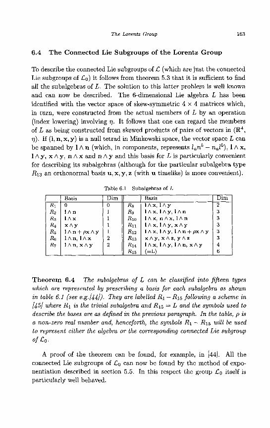
The Lorentz Group 163
6.4 The Connected Lie Subgroups of the Lorentz Group
To describe the connected Lie subgroups of C (which are just the connected Lie subgroups of LO) it follows from theorem 5.3 that it is sufficient to find all the subalgebras of L. The solution to this latter problem is well known and can now be described. The 6-dimensional Lie algebra L has been identified with the vector space of skew-symmetric 4 x 4 matrices which, in turn, were constructed from the actual members of L by an operation (index lowering) involving 77. It follows that one can regard the members of L as being constructed from skewed products of pairs of vectors in (R4, q). If (1, n, x, y) is a null tetrad in Minkowski space, the vector space L can be spanned by 1 A n (which, in components, represents l,nb - nalb), 1 A x, 1 A y, x A y, n A x and n A y and this basis for L is particularly convenient for describing its subalgebras (although for the particular subalgebra type R13 an orthonormal basis u, x, y, z (with u timelike) is more convenient).
Table 6.1 Subalgebras of L
Basis 0 I A n 1 A x
1 A n + px A y l A n , 1 A x I A n , x A y
X A Y
- Dim 0 1 1 1 1 2 2
- - Dim 2 3 3 3 3 3 4 6
-
-
Theorem 6.4 The subalgebras of L can be classified into fijleen types which are represented by prescribing a basis for each subalgebra as shown in table 6.1 (see e.g.[&/). They are labelled R1- Rls following a scheme in 1451 where R1 is the trivial subalgebra and Rl5 = L and the symbols used to describe the bases are as defined in the previous paragraph. I n the table, p is a non-zero real number and, henceforth, the symbols R1 - R15 will be used to represent either the algebra or the corresponding connected Lie subgroup of Lo.
A proof of the theorem can be found, for example, in [44]. All the connected Lie subgroups of CO can now be found by the method of expo- nentiation described in section 5.5. In this respect the group LO itself is particularly well behaved.
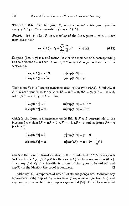
164 Symmetries and Curvature Stmcture in General Relativity
Theorem 6.5 every f E LO is the exponential of some F E L).
Proof. from section 5.5
T h e Lie group LO is a n exponential Lie group (that is
(cf [44]) Let F be a member of the Lie algebra L of LO. Then
O0 tS exp(tF) = 14 + - F" (t E R)
S! s=l (6.13)
Suppose (1, n, x, y) is a null tetrad. If F is the member of L corresponding to the bivector 1 A n then 1F = -1, nF = n, xF = y F = 0 and so from section 5.5
l[exp(tF)] = e-tl x[exp(tF)] = x n[exp(tF)] = etn YbP( tF ) ] = Y
Thus exp(tF) is a Lorentz transformation of the type (6.8a). Similarly, if F E L corresponds to x A y then 1F = nF = 0, xF = y , y F = -x and, with a m = x + iy, mF = -im,
l[exp(tF)] = 1 n[exp(tF)] = n
m [ e x p ( t ~ ) ] = e - i t m m [ e x p ( t ~ ) ] = eitm
which is the Lorentz transformation (6.8b). If F E L corresponds to the bivector 1 A y then 1F = xF = 0, y F = -1, nF = y and so (since Fk = 0 for Ic 2 3)
l[exp(tF)] = 1 y[exp(tF)] = y - tl
x[exp(tF)] = x 1 2
n[exp(tF)] = n + ty - -t21
which is the Lorentz transformation (6.8d). Similarly if F E L corresponds to 1 A n + p(x A y) (0 # p E R) then exp(tF) is the screw motion (6.812). Since any f E LO f # identity is of one of the types (6.8a)-(6.8d) and
0
Although LO is exponential not all of its subgroups are. However any 1-parameter subgroup of Lo is necessarily exponential (section 5.5) and any compact connected Lie group is exponential [37]. Thus the connected
exp(0) is the identity the proof is complete.
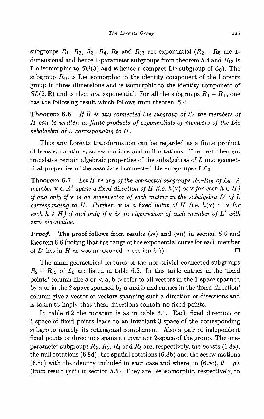
The Lorentz Group 165
subgroups R1, Rz, R3, R4, R5 and R13 are exponential (R2 - Rs are 1- dimensional and hence 1-parameter subgroups from theorem 5.4 and R13 is Lie isomorphic to SO(3) and is hence a compact Lie subgroup of Lo). The subgroup Rlo is Lie isomorphic to the identity component of the Lorentz group in three dimensions and is isomorphic to the identity component of SL(2,R) and is then not exponential. For all the subgroups R1 - R15 one has the following result which follows from theorem 5.4.
Theorem 6.6 If H is any connected Lie subgroup of LO the members of H can be written as finite products of exponentials of members of the Lie subalgebra of L corresponding to H .
Thus any Lorentz transformation can be regarded as a finite product of boosts, rotations, screw motions and null rotations. The next theorem translates certain algebraic properties of the subalgebras of L into geomet- rical properties of the associated connected Lie subgroups of LO. Theorem 6.7 Let H be any of the connected subgroups Rz-R15 of Lo. A member v E R4 spans a fixed direction of H (i.e. h(v) 0: v for each h E H ) if and only if v is an eigenvector of each matrix in the subalgebra L‘ of L corresponding to H . Further, v is a fixed point of H (Le. h(v) = v for each h E H ) i f and only i f v is an eigenvector of each member of L’ with zero eigenvalue.
Proof. The proof follows from results (iv) and (vii) in section 5.5 and theorem 6.6 (noting that the range of the exponential curve for each member
0
The main geometrical features of the non-trivial connected subgroups Rz - R15 of LO are listed in table 6.2. In this table entries in the ‘fixed points’ column like a or < a, b > refer to all vectors in the 1-space spanned by a or in the 2-space spanned by a and b and entries in the ‘fixed direction’ column give a vector or vectors spanning such a direction or directions and is taken to imply that these directions contain no fixed points.
In table 6.2 the notation is as in table 6.1. Each fixed direction or 1-space of fked points leads to an invariant 3-space of the corresponding subgroup namely its orthogonal complement. Also a pair of independent fixed points or directions spans an invariant 2-space of the group. The one- parameter subgroups Rz, R3, R4 and R5 are, respectively, the boosts (6.8a), the null rotations (6.8d), the spatial rotations (6.8b) and the screw motions (6 .8~) with the identity included in each case and where, in (6.8c), 8 = pX (from result (viii) in section 5.5). They are Lie isomorphic, respectively, to
of L’ lies in H as was mentioned in section 5.5).
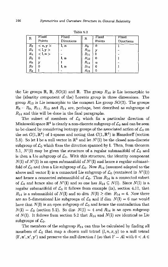
166
R2 R3 R4 R5 R S Y R7 Rn
Symmetries and Curvature Structure in General Relativity
Fixed Fixed P'ixed Points Directions Points <x,y > 1, n Rg 0 <l,y > Rio Y < l , n > Rii 1 0 1, n R12 0
R
1 R13 u 0 1, n R14 0 1 Ris 0
I Fixed Directions
~1
' -
1
1
the Lie groups R, R, SO(2) and R. The group Rlo is Lie isomorphic to the (identity component of the) Lorentz group in three dimensions. The group R13 is Lie isomorphic to the compact Lie group SO(3). The groups Rs - Rg, R11, Rlz and R14 are, perhaps, best described as subgroups of R14 and this will be done in the final paragraphs.
The subset of members of LO which fix a particular direction of Minkowski space R4 is clearly a non-discrete subgroup of LO and can be seen to be closed by considering isotropy groups of the associated action of LO on the set G(1,R4) of 1-spaces and noting that G(1,R4) is Hausdorff (section 5.8). So let 1 be a null vector in R4 and let "(1) be the closed non-discrete subgroup of Lo which fixes the direction spanned by 1. Then, from theorem 5.1, "(1) may be given the structure of a regular submanifold of LO and is then a Lie subgroup of LO. With this structure, the identity component N(l) of "(1) is an open submanifold of "(1) and hence a regular submani- fold of LO and thus a Lie subgroup of LO. Now R14 (assumed adapted to the above null vector 1) is a connected Lie subgroup of LO (contained in "(1)) and hence a connected submanifold of LO. Thus R14 is a connected subset of LO and hence also of "(1) and so one has R14 N(1). Since N(l) is a regular submanifold of LO it follows from example (ix), section 4.11, that R14 is a submanifold of N(l) and so dim N(l) 2 dim R14 = 4. Now there are no 5-dimensional Lie subgroups of LO and if dim N(l) = 6 one would have that N(1) is an open subgroup of LO and hence the contradiction that N(1) = LO (section 5.2). So dim N(l) = 4 and R14 is an open subgroup of N(1). It follows from section 5.2 that R14 and N(l) are identical as Lie subgroups of LO.
The members of the subgroup R14 can thus be calculated by finding all members of LO that map a chosen null tetrad (1, n, 2, y) to a null tetrad (l', n', x', y') and preserve the null direction 1 (so that 1' = A1 with 0 < A E
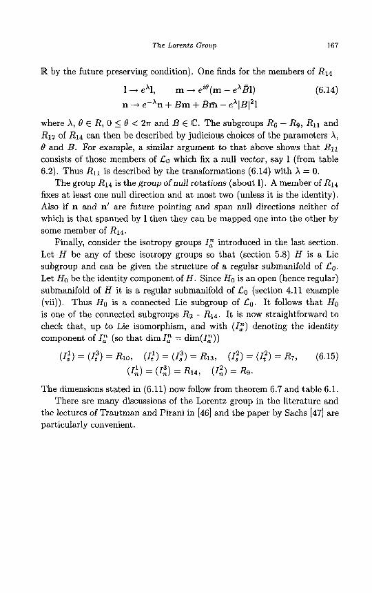
The Lorentz Group 167
I[$ by the future preserving condition). One h d s for the members of R14
I -+ 2 1 , m + eie(m - eXBI) (6.14) n -+ e-'n + Bm + Bm - eXIBI21
where A, 8 E R, 0 5 8 < 2n and B E C. The subgroups R6 - Rg, R11 and R12 of R14 can then be described by judicious choices of the parameters A, 8 and B. For example, a similar argument to that above shows that R11
consists of those members of LO which fix a null vector, say 1 (from table 6.2). Thus R11 is described by the transformations (6.14) with A = 0.
The group R14 is the group of null rotations (about 1). A member of R14
fixes at least one null direction and at most two (unless it is the identity). Also if n and n' are future pointing and span null directions neither of which is that spanned by 1 then they can be mapped one into the other by some member of R14.
Finally, consider the isotropy groups I," introduced in the last section. Let H be any of these isotropy groups so that (section 5.8) H is a Lie subgroup and can be given the structure of a regular submanifold of LO. Let HO be the identity component of H . Since HO is an open (hence regular) submanifold of H it is a regular submanifold of LO (section 4.11 example (vii)). Thus HO is a connected Lie subgroup of LO. It follows that HO is one of the connected subgroups Rz - R14. It is now straightforward to check that, up to Lie isomorphism, and with (I,") denoting the identity component of I," (so that dimI," = dim(1,"))
(I:) = ( I f ) = Rio, (1;) = (12) = R13, (I:) = (I:) = R7, (6.15)
(I:) = (I:) = R14, (I:) = Rg.
The dimensions stated in (6.11) now follow from theorem 6.7 and table 6.1. There are many discussions of the Lorentz group in the literature and
the lectures of Trautman and Pirani in 146) and the paper by Sachs 1471 are particularly convenient.

This page intentionally left blank
Chapter 7
Space-Times and Algebraic Classification
7.1 Space-Times
It is not the purpose of this book to enter into a logical or historical de- velopment of Einstein’s field equations of general relativity theory. More detailed discussion of these equations can be readily found elsewhere (see, e.g. [48]-[51]). This section will thus content itself with the mathematics of the space-time as interpreted in classical general relativity and some elementary knowledge of general relativity will necessarily be assumed.
A space-time is a pair ( M , g ) where M is a 4-dimensional, smooth, connected, Hausdorff manifold and g a smooth Lorentz metric on M of signature (-1,1,1,1). The members of M are referred to as points or events. Any metrical property of a tensor etc. at m E M (eg. “null”, %on-null”) will always be assumed to refer to the Lorentz metric g(m). A global condition such as a “timelike vector field” will be a vector field which is timelike at each point where it is defined. The definition of a space-time requires the following remarks.
i) The usual agreement, in general relativity is that “information” is trans- mitted along piecewise differentiable curves whose tangent vector, where defined, is timelike or null. Thus if M consisted of more than one path component the events in one such component could have no influence on the events in the other and in this sense, such components would have independent physics. Since, for a manifold with its natural manifold topology, path connectedness and connectedness are equivalent state- ments, then in order to have a single physics for M one assumes M is connected.
ii) The assumptions that M is 4-dimensional and Hausdorff are usually (and perhaps uncomfortably) attributed to “experience”. The existence
169
170 Symmetries and Curvature Structure in General Relativity
of the Lorentz metric g then implies that M is paracompact [32]. iii) The assumption that M is smooth is taken here mainly for convenience.
It is mitigated by the fact (see section 4.5) that every complete C' atlas (T L 1) of M contains a smooth atlas. The choice of a smooth metric g for M is also one of convenience and, of course, would make no sense unless M was smooth.
iv) The symmetric Levi-Civita connection arising from g , and its associated curvature tensor are usually referred to as the connection and curvature (Riemann tensor) of M . In this sense one calls a space-time flat if the curvature is identically zero on M (and so M is not flat if the curvature is not identically zero on M ! ) and non-flat if the curvature does not vanish over a non-empty open subset of M (i.e. the curvature is non-zero at each point of an open dense subset of M ) .
v) Suppose there exists a smooth diffeomorphism f : M --f M . Then f * g and g are both Lorentz metrics for M . Although g and f * g need not be the same metric for M , the space-time ( M , g ) and ( M , f * g ) are isometric under f and, for the present purposes, identical. Formally one should, perhaps, identify such space-times and work within an equivalence class of such an equivalence relation. For the present purposes, however, a space-time will continue to be M together with a particular choice of Lorentz metric g on M .
One problem which concerns the global topology of a space-time manifold M is the question of whether or not it is simply connected. Since one may always choose a coordinate domain to be simply connected, local problems are indifferent to this (global) property of M . In fact simply connectedness will not be part of the definition of a space-time but will be added as an extra assumption from time to time in order to be able to deal with certain global mathematical constructions. It is remarked here that it is not hard to show from the work of section 4.14 that any space-time is isometric to the quotient manifold of a simply connected space-time. For if A? is the universal covering manifold of M with covering map p : A? 4 M let f : M 4 A?/- and i : A? -+ A?/- be the maps described in section 4.14 with i = f o p. Then g1 = p*g and g2 E ( f P 1 ) * g are metrics on A? and A?/-, respectively, (and then ( M , g ) and (A? / - ,gZ) are isometric) and g1 = p*g = (f-' o i ) * g = i *gz . One result of interest (especially in the thermodynamical aspects of general relativity) is that if M is a simply connected space-time then M admits a global smooth nowhere zero timelike vector field and hence a consistent choice of the future direction of time on

Space- Times and Algebraic Classification 171
M . This follows [52] from the existence of a 1-dimensional distribution on M guaranteed by theorem 4.15.
It is remarked that one normally chooses the space-time manifold M to be not compact (otherwise one has closed timelike curves and the associated philosophical problems [53]). Given that M is also paracompact one then has the existence on M of a global, nowhere zero, smooth vector field X [54] which, together with the positive definite metric on M guaranteed by theorem 4.14, leads to a Lorentz metric on M constructed from the 1-dimensional distribution determined by X and for which X is timelike everywhere.
The gravitational field is interpreted through the metric g and so field equations restricting g are required. These are the Einstein field equations given in each coordinate system of A4 by (see, e.g. [48])
where (section 4.16) the Rab are the Rcci tensor components, R(=: Rabgab) is the Ricci scalar, A is a constant called the cosmological constant and the tensor T is the energy-momentum tensor with components Tab(= T b a )
about which more will be said later. There are good reasons for supposing IAl very small and in this book the assumption A = 0 will be made unless otherwise specified. The field equations (7.1) thus reduce to
where G is the Einstein tensor. Using a semi-colon to denote a covariant derivative with respect to the space-time connection, the Bianchi identities Rab[,-die] = 0 (see (4.36)) are easily shown to contract to the equivalent statements
(7.3) b Gab;b 0 , Ta ;b = 0
The second of these is usually referred to as the conservation law for T . The energy-momentum tensor is usually taken as formally representing
the sources of the gravitational field. The more commonly used energy- momentum tensors will now be briefly discussed.
7.1.1 Electromagnetic fields
An electromagnetic field in space-time is described by the current density vector field j with components j a , representing the electric charge and
172 Symmetries and Curvature Structure in General Relativity
current distribution and the resulting electric and magnetic fields which are combined into the Maxwell tensor (or Maxwell bivector - see section 7.2) F with components Fab(= -Fba). Maxwell's equations are then
( 7 . 4 )
The contribution of such a Maxwell field to the energy-momentum tensor is then given by
T a b = &(FacFbc - i F c d F C d g a b ) . (7.5)
If (7.5) is the total energy-momentum tensor, one usually refers to the gravitational field as an Einstein-Maxwell (or an electrovac) field.
7.1.2 Fluid Space-Times
Suppose the source of the gravitational field is a viscous fluid. The latter is described by its coefficients of dynamic viscosity 77 and bulk viscosity <, a unit timelike vector field u representing the Auid flow, its energy density p with respect to u, its isotropic pressure p , its shear tensor cr, its expansion 0 and its heat Aow vector field q. These quantities satisfy uaua = -1, uaqa = 0, Dab = Uba, uaa = o and UabUb = o and the resulting energy- momentum tensor is
T a b = ( p - <e -k p ) u a u b -k ( p - <@)gab - %'gab -k 2u(aqb). ( 7 . 6 )
There are several special cases to consider here and which result when some of the above physical quantities associated with the fluid take special values. Perhaps the most important is the case of a perfect A uid. This arises when < = 77 = 0 and q = 0 and T reduces to
T a b = ( p -k p ) u a u b + Pgab (7.7)
7.1.3 The Vacuum Case
This is a rather important case for general relativity and occurs when T = 0 on M . Then M is called a vacuum space-time and Einstein's field equations reduce to either of the following two equivalent statements
Rat, = 0, Gab = 0 ( 7 . 8 )
If T E 0 over some non-empty open subset U of M then U with its open submanifold structure and induced metric is called a vacuum region of M.
Space-Tames and Algebraic Classification 173
Further details regarding the postulates of general relativity and details of the field equations can be found in [48] whilst a comprehensive list of exact solutions of (7.1), (7.2) and (7.8) is contained in [55]. A full discussion of the algebraic structure of the general energy-momentum tensor and of the particular examples above will be given later in this chapter.
The energy-momentum tensor is usually subject to the so-called energy conditions that at each p E M and for each timelike vector u E T,M
(i) TabuaUb 2 0, (ii) Tabub is not spacelike (7.9)
By continuity, each condition is still true if u is null. The first condition expresses the non-negativity of the local energy-density of the field for any observer (represented by u) and the second the non-spacelike nature of the local energy flow vector. Condition (i) alone is sometimes referred to as the weak energy condition and (i) and (ii) together as the dominant energy conditions [48]. The restrictions they impose on T will be discussed later.
There is a useful decomposition of the curvature tensor of M given at P E M by [561 7 [571
Rabcd = Cabcd + Eabcd + i R Gabcd (7.10)
where C is the Weyl tensor and
Eabcd = Ra[cgd]b + Rb[dgc]a Gabcd = ga[cgd]b (7.11)
and where f i a b s R a b - + & j a b is the tracefree (part of the) Ricci tensor (Baa = 0). For a fixed g the expression (7.11) for E at p E M is a linear one-to-one relation between E and R (since ECacb = Rat,) and, in particular, E = 0 % R = 0 % Rat, = $Rgab which is equivalent to M satisfying the Einstein space condition (section 4.16) at p. The decomposition (7.10) will be further explored later.
7.2 Bivectors and their Classification
Let ( M , g ) be a space-time and p E M . A second order skew-symmetric tensor F (at p ) with components Fab(= -Fba) is called a bivector (at p ) . The set B ( p ) of all bivectors at p is thus a 6-dimensional real vector space. If F E B(p) one can define the dual of F , denoted by * F , by
1 2 *Fat, = -EabcdFCd (7.12)
174 Symmetries and Curvature Structure in General Relativity
where is the usual pseudotensor (see, e.g. [51]) and * is the duality operator. Thus 6&d is completely skew symmetric and, with g denoting det(gab) (this should cause no confusion with the metric itself), eabcd is ob- tained from €abed by the usual index raising and = (-g)i = -61234.
[It is remarked that unless M has the extra property of being orientable (which will not be assumed in this text) there are problems with a global definition of the dual. However, such a definition is satisfactory in an ap- propriately chosen coordinate domain and where such a domain is required it will be assumed so chosen without further comment.] These quantities and hence * F are only tensors under coordinate transformations where the transformation matrix has positive determinant. * Fab is obtained from *Fab by the usual raising of indices with g. If F and H are bivectors then standard formula (511 associated with the pseudotensor give
**Fat, = -Fab (7.13)
FabFab = -*Fab*Fab (7.14)
(7.15)
Since Fab is skew symmetric it is a standard result in algebra that the rank of the matrix Fab is even and hence, if F # 0, equal to two or four. If F has rank 2 it is called simple and if it has rank 4 it is called non-simple. Because the rank of a non-zero bivector F can never be three the existence of k E T,M, k # 0, satisfying Fabkb = 0 is then equivalent to F being simple. If F is simple it follows that the components Fab may be chosen with two rows (and hence two columns) consisting entirely of zeros. From this it follows by inspection that there exist two independent covectors r and s at p such that Fab = rash - sarb = 2r[,sb]. The 2-space at p spanned by the vectors ra and sa is then easily checked (by considering orthogonal complements) to be well defined independently of the choice of r and s and is called the blade of F . If Ic is any vector at p orthogonal to this blade (i.e. orthogonal to every member of this blade) then Fabkb = 0 and conversely. Also, it follows from this that if F is simple and written in the above form then *Fabrb = *FabSb = 0 and so * F is simple and can be written as * F = 2riasb1 for independent vectors T I a , sIa orthogonal to the blade of F . Thus F is simple if and only if * F is simple and then their blades are orthogonal complements of each other. One now has the following theorem
Theorem 7.1 The following statements are equivalent for a non-zero
Space- Times and Algebraic Classification 175
bivector F at p .
i) F is simple. ii) There exists k E T p M , k # 0 , such that Fabkb = 0. iii) There exist independent members r, s E Tp* M such that Fab = %[ash]. iv) * F is simple. V ) *FabFbC = 0. vi) *FabFab = 0.
U i i ) F[abFc]d = 0.
Proof. The equivalence of conditions (i), (ii), (iii) and (iv) was estab- lished above. That these conditions together imply (v), (vi) and (vii) is then straightforward as are the implications (v) (vi) from (7.15). Now since F # 0, there exist k E T i M , k # 0 , such that FbCkc # 0 and so immediately one has (v) H (iv). Finally if (vii) holds choose q E T,M, q # 0, such that Fcdqd = q: # 0 and contract the condition (vii) with qd to obtain FIabqlC] = 0. A contraction with t E T p M satisfying tag: # 0 then
0 shows that (iii) holds. This completes the proof.
The set of simple bivectors at p can be further classified into three types, spacelike, timelike and null, according as the corresponding blade of the bivector is a spacelike, timelike or null 2-space at p , respectively. It follows that the dual of a timelike bivector is spacelike and vice-versa and that the dual of a null bivector is null (section 6.1). It is clear that for any simple bivector, when written in the form (iii) of theorem 7.1 above, r and s may be chosen to be orthogonal. Also, a simple bivector uniquely determines its blade and, conversely, if a 2-space at p is the blade of the bivectors Fl and F2 then Fz = XFl (A E R). It is also useful to note that if a bivector F # 0 at p satisfies F[,bk,] = 0 for k E T i M , k # 0 , then F is simple and its blade contains k. This follows by contracting this last equation with wc for w E T p M and waka # 0. Another remark is that it is easily checked that Eabcd;e = 0 and so the covariant derivative and dual operations on bivectors are interchangeable.
Theorem 7.2 bivector F at p .
The following statements are equivalent for a non-zero
i) F is null. ia) There exists k E T p M , k # 0 , such that Fabkb = *Fabkb = 0. iii) FabFab = *FabFab = 0.
176 Symmetries and Curvature Structure an General Relativity
Proof. If (i) holds one can check from the previous discussion of null 2-spaces in section 6.1 that (ii) holds with k spanning the principal null direction of the blade of F (and * F ) . Conversely (ii) + (i) because (ii) shows that the blades of F and * F , although orthogonal complements, do not span T,M and hence that these blades must be null. Further, if (i) holds then, again consulting the previous discussion of null 2-spaces, one may write (assuming an appropriate orientation of x and y ) Fab = 21[,xb], *Fat, = -21[,yb] with 1 null, x and y spacelike and l a x , = laya = xaya = 0. The condition (iii) is then immediate. Finally if (iii) holds the second condition in (iii) and the previous theorem show that F is simple. So write F a b = 2r[,sb] and * F a b = 2r;,;k1. with the pairs (r,s) and (r',s') chosen orthogonal. Then the first condition in (iii) and (7.14) give
(rara)(s,sa) = (rbr'")(s~s'") = o (7.16)
so one of r and s, say r and one of r' and s', say r', is null. But T a r t a = 0 0
It should be noted that the condition (ii) in the last theorem implies that k is null and unique up to a scaling. In fact k spans the (necessarily null) direction in which the orthogonal null blades of F and * F intersect and this is called the (repeated) principal null direction of F (and * F ) .
Let x and y be unit orthogonal spacelike vectors at p E M and suppose they are extended at p to a null tetrad 1 , n, x , y and also to a orthonormal tetrad x , y , z , t with 1 and n null, z unit spacelike, t unit timelike and f i z = 1 + n, f i t = 1 - n. Then two bases for the 6-dimensional vector space B(P) of bivectors at p may be conveniently constructed from these tetrads. As a notational convenience the general simple bivector 2r[,sb] will be denoted by the symbol r A s. These bases are
and so r and r' are proportional. It follows that F is null.
F ~ = Z A X F ~ = ~ A Y F 3 = x A y (7.17)
F 4 = n A x F 5 = n A y F 6 = 1 A n
and
G ~ = X A Y G ~ = X A Z G 3 = y A z (7.18)
G 4 = t A x G 5 = t A y G 6 = t A z
It should be noted that, up to signs, ( F ' , F 2 ) , ( F 3 , F 6 ) , ( F 4 , F 5 ) , (G', G 6 ) , (G2, G 5 ) and (G3, G4) are dual pairs. The bivectors F 1 and F 2 are null with principal null direction (spanned by) 1, F4 and F5 are null with principal
Space- Times and Algebraic Classification 177
null direction n, F 3 , G1, G2 and G3 are spacelike and F 6 , G4, G5 and G6 are timelike. In fact, the way the null and spacelike bivectors are written above is typical for their type. For a timelike bivector there are two typical ways of writing it, namely as F6 or as G4 (G5 or G6). A timelike bivector has a (timelike) blade containing exactly two distinct null directions. They are called the principal null directions of the bivector.
So far only real bivectors have been discussed. Although no formal provision has been made for defining complex second order skew-symmetric tensors (complex bivectors) on a manifold this will informally be assumed. So a complex bivector will be regarded as an object at p whose real and imaginary parts are real bivectors in the sense defined above. The set of complex bivectors at p will be denoted by CB(p) and is clearly a 6- dimensional complex vector space (the complexification of B (p)-see section 2.3). This vector space has two important subspaces denoted by S+(p) and S-(p) which, with the duality operation defined for members of CB(p) by (7.12), are defined by
H E S+(p) @ * H = -iH, H E S-(p) ++ * H = iH (7.19)
If one writes H = A + iB, A , B E B(p) then it follows from (7.19) that H E S+(p) H B = * A and that H E S-(p) w B = -*A. Thus the members of S+(p) are precisely those complex bivectors of the form F+i*F and those in S-(p) precisely those of the form F - i*F for a real bivector F . Thus the members of S+(p) and S-(p) are each uniquely associated with a real bivector in a natural way and so denote members of S+(p) as
F and members of S - ( p ) as F where (cf.[47]) +
+ F = F + i * F p = F - i * F (7.20)
for a real bivector F . Clearly F and F are conjugates. Members of S+(p) are called self-dual and members of S - ( p ) anti self-dual.
Any complex bivector H at P can be written as the sum of a member of S+(p) and a member of S - ( p ) in exactly one way
+
1 1 2 2
H = - (H + i *H) + - ( H - i *H) (7.21)
with H + i*H E S+(p) and H - i*H E S-(p) . It then follows easily that CB(p) is the direct vector space sum (section 2.3)
CB(P) = S+(P) Cr3 s-(P> (7.22)
178 Symmetries and Curvature Structure in General Relativity
Now any F E B(p) can, from (7.17), be written as F = E f f k F ' (1 5 k 5 6, alc E R) and so any F E S + ( p ) can be written as F = C a k ( F k + i * F k ) and any F E S-(p) as fi = ak(Fk - i*Fk)) . Recalling the dual pairing in the bases (7.17) and (7.18) one easily sees how to choose bases for S + ( p ) and S-(p) each consisting of three members and so dim S+(p) = dims-(p) = 3 (as complex vector subspaces of CB(p)).
The maps B(p) -+ B(p) given by d : F --+ * F and d' : F .+ -*F are linear maps on and, in fact, isomorphisms of B ( p ) . They have the property that d2 = dI2 = -1 where 1 is here the identity map on B(p). Hence each gives rise to a complex structure on B(p) (section 2.3) and hence to the complex vector spaces S-(p) and S+(p). A traditional (and useful) way of writing the basis for S+(p) is, using (7.17)
+ +
V = 2-' /2(F1 + i *F1) , U = 2-1/2(F4 + i *F4) , (7.23) M = ( F 6 + i *F6)
Then with the null tetrad appropriately oriented one has [47]
Vab = f i ( l [axb] - i l [ a Y b ] ) = 2 l [ a m b ]
Uab = f i (n [axb] + i n [ a Y b ] ) = 2n[,mb]
Mab = 21[anb] + 2iz[ayb] = 2 l [ a n b ] + 2 m [ a m b ]
(7.24)
(7.25)
(7.26)
where the complex null tetrad (1, n, m, 6) has been introduced with m = 2-1/2(x + i y ) (so that mama = fiama = 0, mafia = 1). A basis for S - ( p ) then consists of the conjugates v, U and M. One easily finds the following relations between V , U , M , v, U and M
UabVab = Oabvab = 2 MabMab = MabMab = -4 (7.27)
with any other such contraction between any two of these six complex bivectors equal to zero.
The orthonormal and null tetrads ( x , y , z , t) and (1, n, 2, y ) and the com- plex null tetrad (1, n, m, f i ) each satisfy a completeness relation linking it with the metric g ( p ) at p . They are

Space-Times and Algebraic Classzfication 179
These are understood in the following sense; if any of these relations hold, the covectors appearing on the right hand side constitute a tetrad of the appropriate type, and conversely. For example, if (I, n, x , y ) is a null tetrad let Sab denote the right hand side of (7.29). Then, clearly Sablb = l a , sabnb = n,, &bXb = x a , &byb = Ya . Hence for any k E T p M &bkb = ka and SO Sab = gab and (7.29) holds. Conversely if (7.29) holds then clearly 1, n , x and y are a basis for T,M because if k E T p M , a contraction of (7.29) with kb shows that they span T,M. Next, successive contractions of (7.29) with lb , nb, xb and y b show that lana = xaxa = yaya = 1 and that all the other inner products between these basis vectors vanish. Hence ( I , n, x , y ) is a null tetrad at p . The other proofs are similar.
Now consider the tensor G at p with components Gabcd given by (7.11). This has the following properties for any bivectors F, H E B(p)
It is clear that G acts as a metric on the vector space B ( p ) according to the (coordinate independent) rule G(F, H ) = G ( H , F ) = FabHab. Also the basis (7.18) is such that, if re-defined by Gk = 2-lI2Gk (1 5 k 5 6), it satisfies
with all other inner products zero. Hence G is a metric on B(p) with signature (+ + + - --) and Sylvester canonical matrix equal to diag(ll1- 1 - 1 - 1). In this notation and using theorem 7.1 a (real) bivector F is simple if and only if G(F, * F ) = 0 and, given it is simple, it is then spacelike, timelike or null according as G(F, F ) is positive, negative or zero. G is sometimes referred to as the bivector metric. There is a completeness relation for bivectors. First one notes that the complex bivectors U , V and M satisfy
1 (7.33)
1 . 2 Gabcd + -tEabcd = VabUcd f UabVcd - SMabMcd
the proof being essentially the same as that for the space-time metric com- pleteness relations above. By taking the real part of (7.33) one obtains the desired relation in terms of G and the real and imaginary parts of U , V and
M (ie. the real bivectors F1, . . . , F 6 ) . It is noted here that if F = F + i*F is in S+(p) with F E B(p) then, informally extending the metric G to
+
180 Symmetries and Curvature Stmcture in General Relativity
complex bivectors, one has
+ + + + G ( F , F ) = FabFab = 2(FabFab + iFab*Fab) (7.34)
+ + and so, from theorems 7.1 and 7.2, F is null if and only if G ( F , F ) = 0
and F is simple if and only if G ( F , F ) E R. A complex self dual bivector
F = F + i*F is called null if F (and hence also * F ) is null. The common principal null direction of F and * F is then called the (repeated) principal
null direction of F . So far, little has been said about real non-simple bivectors. To deal with
these first let ( I , n, m, a) be a complex null tetrad and F any real bivector at p. Under a null rotation about 1 at p (section 6.2) the tetrad (l,n,m,fi) is changed to, say, (Z', n', m', a') where, from (6.14)
+ + +
+
1' = Al , m' = eie(m - ABI) (7.35) n' = A-'n + Bm + Ba - A B B l
( A , @ € & A > 0 , B E C )
The corresponding members U', V' and M' of CB(p) defined as in (7.24)- (7.26) (but in terms of the primed tetrad components) satisfy
V' = M' = 2ABV + M (7.36) u' = ~ ~ 2 ~ i e v + B p M + A-leieU
+ Construct the complex self-dual bivector F = F +i*F corresponding to the real bivector F and write
+ F = F i V ' f F;M' + FiU' = F1V + F2M + F3U (7.37)
for F:, . . . , F3 E C, the intention being to choose U , V , M so that the
expression for F in terms of them is, in some sense, especially simple. A substitution of (7.36) into (7.37) and then equating coefficients of U , V , M gives
+
FI = Ae-z'F; + 2ABF; + AB2eieFi (7.38a) F2 = F; + Beie% (7.3813) F~ = A - ' ~ ~ ~ F ; (7.38~)
Space-Times and Algebraic Classzficataon 181
+ Suppose now that F is not null (equivalently F is not null). Suppose F; = 0
in the above expression for F . Then F3 = 0. If also Fi = 0 then Fz = 0
and the contradiction that F(= F I V ) is null is achieved. Hence, if Fi = 0, Fi # 0. Then (7.38a) shows that there exists B E 6‘ such that F1 = 0 and
so F = F2M. If Fi # 0 then (7.38a) shows that there exists a value of B for which F1 = 0. Thus one achieves a complex null tetrad, say (1, n, m, f i ) , in which FI = 0. Then a null rotation, this time about the null vector n
(and again remembering that F is not null), yields a complex null tetrad
in which F1 = F3 = 0 and again one has F = F2M. Taking real parts one gets for any non-null real bivector F the expression
+ +
t
+ +
Fab = 2Ql[anb] + 2px[aYb] (a, p E R) (7.39)
in terms of a real null tetrad (1, n, x, y ) . If F is spacelike a = 0 and if F is timelike p = 0 and previous results are recovered. If F is non-simple Q # 0 and ,B # 0 and one achieves a convenient expression for F .
A real or complex vector v at p is an eigenvector of F E C B ( p ) with eigenvalue X E @. if uaFab = Xub and the 1-dimensional subspace of C4 spanned by u is called an eigendirection of F . Thus, for the real bivector F in (7.39), 1 and n span real null eigendirections of F with eigenvalues -a and +a respectively and m and rii span complex null eigendirections of F with eigenvalues -ip and +ip, respectively. I t is then clear that, just as a simple (null or non-null) real bivector determines its blade, a non-simple real bivector determines an orthogonal pair of 2-spaces, one timelike (spanned by 1 and n and which are defined to span the principal null directions of F ) and one spacelike (spanned by x and y) and this pair is unique. They are called the canonical pair of blades of F . The following theorem summarises the situation [58]-[60].
Theorem 7.3 A real bivector F # 0 a t p is nul l if and only if it has a un ique real nu l l eigendirection (and the eigenvalue is necessarily zero) a n d non-nul l if a n d on ly i f it admi t s exactly t w o independent real nu l l eigendi- rections (with eigenvalues e i ther both zero if F i s spacelike o r else dif fering only in sign if F i s t imel ike o r non-simple) .
So far the discussion of the algebraic properties of bivectors has been studied using “canonical” tetrads. Now a discussion through Segre types will be given. It is noted that, on account of the skew-symmetry of F , Fabgab = Faa = 0 and so the sum of the eigenvalues of F is zero. For
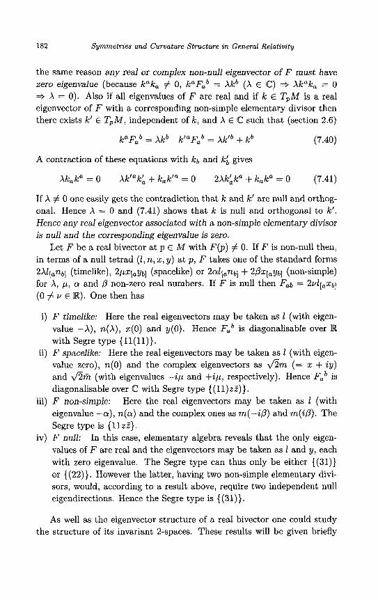
182 Symmetries and Curvature Structure in General Relativity
the same reason any real or complex non-null eigenvector of F must have zero eigenvalue (because kaka # 0, kaFab = Akb (A E C) + Akaka = 0 + X = 0). Also if all eigenvalues of F are real and if k E TpM is a real eigenvector of F with a corresponding non-simple elementary divisor then there exists k' E T p M , independent of k , and A E C such that (section 2.6)
kaFab = Akb klaFab = Akfb + kb (7.40)
A contraction of these equations with kb and k; gives
Akaka = 0 Ak'"kL + kak'" = 0 2AkLka + kaka = 0 (7.41)
If X # 0 one easily gets the contradiction that k and k' are null and orthog- onal. Hence A = 0 and (7.41) shows that k is null and orthogonal to k'. Hence any real eigenvector associated with a non-simple elementary divisor is null and the corresponding eigenvalue is zero.
Let F be a real bivector at p E M with F ( p ) # 0. If F is non-null then, in terms of a null tetrad (1, n, z, y) at p , F takes one of the standard forms 2Xl[,nb] (timelike), 2pq,yb~ (spacelike) or 2Cd[,nb] + 2pz[,yb] (non-simple) for A, p, (Y and p non-zero real numbers. If F is null then Fab = 2 v l [ , Z b ]
(0 # v E R). One then has
i) F timelike: Here the real eigenvectors may be taken as 1 (with eigen- value -A), n(A), z(0) and y(0). Hence Fab is diagonalisable over W with Segre type {11(11)}.
ii) F spacelike: Here the real eigenvectors may be taken as 1 (with eigen- value zero), n(0) and the complex eigenvectors as f i m (= z + iy) and f i m (with eigenvalues -ip and +ip, respectively). Hence Fab is diagonalisable over C with Segre type { (1l)z.Z)).
Here the real eigenvectors may be taken as 1 (with eigenvalue -a), n(a) and the complex ones as m(-iP) and m(ip). The Segre type is {IlzZ).
In this case, elementary algebra reveals that the only eigen- values of F are real and the eigenvectors may be taken as 1 and y, each with zero eigenvalue. The Segre type can thus only be either { (31)) or { (22)). However the latter, having two non-simple elementary divi- sors, would, according to a result above, require two independent null eigendirections. Hence the Segre type is ((31)).
iii) F non-simple:
iv) F null:
As well as the eigenvector structure of a real bivector one could study the structure of its invariant 2-spaces. These results will be given briefly
Space- Times and Algebraic Classification 183
here and are easily proved using tetrad techniques. Let F be a real bivector at p . A 2-space W C TpM is called an invariant Bspace of F if whenever ra is in W so also is raFab. Any such bivector admits an invariant 2-space and if W is an invariant 2-space of F so also is the orthogonal complement of W . If W is a null invariant 2-space of F the unique null direction in W is a real null eigendirection of F . If W is a timelike invariant 2-space then the two real null directions contained in W are real null eigendirections of F . It is a straightforward exercise to link the existence of invariant 2-spaces of F with the latter’s Segre type.
There is a map fe : B(p) - B(p) given for F E B(p) and 0 5 0 < 27r by
F -+ fe(F) = cos0F - sin0 *F (7.42)
and called a duality rotation (through the angle 0). It can also be written
in terms of the complex self-dual bivectors F and F’ corresponding to F + + + and f o (F) , respectively, as F - F’ = eieF. Clearly if F is null then so is f e ( F ) for each 0 but if F is spacelike or timelike, f e ( F ) is, in general, non-simple. If F is non-simple then there exists 0 such that f e ( F ) is simple and choices of 0 exist such that f e (F ) is spacelike or timelike. The blades of these latter bivectors are the canonical pair of blades of F as in (7.39).
The set B(p) of real bivectors at p E M can be regarded as the man- ifold and vector space R6 (section 4.3, example (iv)). The set Q’(p) of simple members of B(p) is a subset but not a subspace of B(p) . Let B1, B2 E B(p) be non-zero and consider the equivalence relation N on B(p) given by B1 N B2 @ B2 = XB1,X E R. Thus one obtains the quotient manifold P5R = G(l, R6) of “projective bivectors” (section 4.17). Since the equivalence class under N of a simple bivector consists entirely of simple bivectors one can define the set of equivalence classes Q of Q’ under N ( “projective simple bivectors” ). Now each simple bivector deter- mines its blade uniquely and each such blade determines its corresponding bivector up to a real multiple. Now the set of blades (2-spaces) at p is just the Grassmann manifold G(2,R4). Hence one has a natural injective map 4 : G(2,R4) - P5R (section 4.17) whose range is Q. To obtain a coordinate representative of this map choose a basis of TpM such that a particular member of G(2,R4) is spanned by ( l ,O,z ,y) and (O,l,a,b) for z , y , a , b E R. In the associated Grassmann chart for G(2,R4) and the obvious (Grassmann) chart in P5R = G(1,R6) the map has coordinate representative (z, y, a, b) - ( a , b, -2, -y, zb - ya). Elementary differenti-
+ +
184 S y m m e t r i e s and Curnature Structure in General Relat iv i ty
ation reveals this map to be of rank four and hence an immersion and so Q, which is the range of 4, may be given the structure of a 4-dimensional submanifold of P5R diffeomorphic to G(2,R4) and is, with its topology, compact and connected and is a closed regular (theorem 4.8 (i)) submani- fold of the (Hausdorff) manifold P5W.
7.3 The Petrov Classification
As a preamble to this and other algebraic classifications it is useful to consider at a point p in the space-time A4 those tensors W of type (0, 4) satisfying the algebraic symmetries
W a b c d = -Wbacd = - w a b d c r W a b c d = W c d a b (7.43)
W a b c d -k W a c d b + W a d b c = 0, (@ W a [ b c d ] = 0) (7.44)
the bracketed equivalence in (7.44) following from (7.43). For such a tensor one can define the left dual * W and the right dual W * by
An immediate consequence (cf. (7.13)) is that
** W a b c d = -Wabcd w,*,*,d = -Wabcd (7.46)
Such tensors satisfy the Ruse-Lanczos identity (see, e.g. [61])
* W & -k W a b c d = 2ga[cT/ir,]b -k 2gb[dWc]a (7.47)
where W a b W C a c b (= W b a from (7.44)), m a b W a b - i W g a b , w f W a a
(and hence c?laa = 0). It follows from (7.47) that *W:[bcdl = 0 and a contraction of (7.47) with gbd reveals the equivalent statements
* W & d = --abed (e * W a b c d = W:bcd) * w a b = 0 (7.48)
Next, the following statements are equivalent for W (even if only (7.43) is assumed)
W a [ b c d ] = 0, Wabcd febcd = 0, W * a b a d = 0 (7.49)
Thus if one takes W as the curvature tensor of the space-time one has, apart from the usual symmetries, the relation R*abad = 0
Space- Times and Algebraic Classi f icat ion 185
Now take W as the Weyl tensor C (see section 4.16). Then it follows from (7.47) and the result C a b a d = 0 that
(7.50)
Further one has
and so * C (and hence C") satisfies (7.43). Then applying (7.49) to W(= C * )
using (7.50) yields C*a[bcd] = 0 and to C yields C*abad = 0. Thus if one
defines the complex self-dual Weyl tensor C by +
+ C a b c d = Cabcd i*Cabcd (7.52)
then C satisfies the symmetries (7.43) and (7.44), the relation C a b a d = 0
and the self dual property *C = -iC (the position of * being irrelevant). There is a convenient way of labelling the components of a tensor such
as W above. Allowing capital letters A, B , . . . to take the values 1 , 2 , . . . , 6 one can label a skew-symmetric pair of tensor indices with such a capital letter. Adopting the convention [23]* 1, [31]- 2, [12]- 3, [lo]++ 4, [20]* 5, [30)* 6, W can now be written as WAB and is a symmetric 6 x 6 matrix since WAB = WBA. This notation is referred to as the 6 x 6 notation and the indices A, B , . . . as bivector indices. It was, as far as the author is aware, first used by Kretschmann [3] and will here be applied to the Weyl tensor. The rank of W is defined to be the rank of the matrix WAB.
The Weyl tensor C on space-time is an important geometrical object and a general description of it was given in section 4.16. In the component form C a b c d it is conformally invariant. A very important advance in gen- eral relativity was made by Petrov [62],[63] when he developed an algebraic classification for the Weyl tensor (more precisely he originally devised the classification for the Riemann tensor of a space-time which was an Einstein space). Petrov's work was extended by others in the decade that followed it and contributions by GBhBniau [64], Be1 [65], Debever [66], Pirani [67], Penrose [68], Sachs [47] and Ehlers and Kundt [41] are of particular impor- tance. For vacuum space-times, the Riemann and Weyl tensor are equal and the Petrov classification then applies to the Riemann tensor.
It is remarked here that the tensors Gabcd and fabed used in the pre- vious section have the algebraic properties (7.43) and also from (7.47)
+ + + +
that G&d = *Gab&(= i f a b c d ) . Further, G a p e d ] == 0 (and SO Eabad = o),
186 S y m m e t r i e s and Curva ture S t ruc ture in General Relat iv i ty
G a b a d = $gbd # 0 (and SO Ea[bcd] # 0) and f:bcd = *Eabcd = -2Gabcd . The
complex self-dual tensor G = G + i * G with components Gabcd + &abcd will be found useful later.
A convenient (but certainly not the only) approach to the algebraic classification of the Weyl tensor starts with the idea of an eigenbivector. It should be pointed out that this is an algebraic classification of C and that the details below apply at a single point p E M . A (real or complex)
bivector F E CB(p) is called an eigenbivector of C (respectively, of C) if the first (respectively, the second) equation in (7.53) holds
+
+
C a b c d F C d = X F a b +
(A E @)
C a b c d F C d = @ab ( p E @) (7.53)
and then X (respectively, p ) is the associated eigenvalue. The classification sought is an algebraic (eigenbivector-eigenvalue) classification of the (real) Weyl tensor C when the latter is regarded as a linear map B(p) -+ B ( p ) (i.e. R6 + R6) given by H a b -+ C a b c d H C d . It turns out, however, to be more convenient to change the problem to an equivalent one (and an ob- vious abbreviated notation in which, for example, for a bivector H , CH means C a b c d H C d , will be useful for this purpose). Such an algebraic de- scription of the linear transformation R6 -+ R6 represented by C in terms of matrix similarity can be equivalently described by regarding C as a linear map CB(p) + CB(p) by extending the definition of the original map to complex bivectors. Thus C is now regarded as a linear map C6 -+ C6, the algebraic equivalence, in the above sense, being mentioned in section 2.6. Now if H E CB(p), one has * ( C H ) = *CH = (C*H) = C(*H) . It follows from (7.19) that if H E S+(p) (respectively, S-(p)) then C H E Sf(p) (respectively, S - ( p ) ) . Thus, from (7.22), C is completely described by its obvious restrictions C1 and Cz which are then, respectively, linear maps Cl : S+(p) -+ S+(p) and Cz : S-(p) t S-(p). Then introducing the conjugation operator k : CB(p) -+ CB(p), given by k ( H ) = ff, one has Cz = k o C1 o k - l . It follows that C1 and CZ have identical Jordan forms as linear maps C3 -+ C3 (including degeneracies and with eigenvalues differ- ing only by conjugation). Since s + ( ~ ) and s - ( ~ ) are invariant subspaces of C whose direct sum is CB(p), the Jordan form of C is just the common Jordan form of C1 and Cz “repeated” in an obvious way. This common Jordan form will be taken as the algebraic “type” of C. +
Now consider the complex self-dual Weyl tensor C at p as a linear map
Space-Tames and Algebraic Classification 187
CB(p) -+ CB(p) in the same way as for C. Then
+ H E S+(p) +- CH = (C + iC*)H = CH + iC(*H) = 2CH E S+(p)
+ H E S-(p) =+ CH = (C + iC*)H = CH + iC(*H) = 0 (7.54)
+ Thus C has a range contained in S+(p) and maps S-(p) to zero. Further,
the first equation in (7.54) shows that the restriction of C to S + ( p ) is
simply twice the restriction C1 of C to S+(p) . Thus the Jordan form of C is determined by the Jordan form of its restriction to S + ( p ) which is, apart from the factor 2, identical to that of C1 and hence to the algebraic type of C defined above. Thus the problem of classifying C has been transformed
to the equivalent problem of classifying (the restriction of) C on the 3- dimensional complex vector space S+(p) of complex self-dual bivectors at p . One further transformation of the problem is instructive.
Recalling the 6 x 6 notation mentioned earlier one can, using the sym- metry of the 6 x 6 Weyl tensor, write
+ +
+
M N~ CAB = ( N Q )
(7.55)
where M , N and Q and 3 x 3 real matrices with M and Q symmetric. The symmetry (7.44) for C when written out using (a ,b ,c ,d) = (0,1,2,3) and the 6 x 6 index convention shows that N is tracefree. At this point a frame (in fact an orthonormal frame with respect to g ( p ) ) will be introduced in T,M but the final outcome will be independent of it. In this frame one has gab(p) = diag(-l,1,1,1) = 7)ab and then the identity gaeC&,ad = 0 is written out in terms of the components CAB in this frame. A little algebra shows that these ten conditions are equivalent to the ten restrictions N = N T , Q = -M and trace M = 0 in (7.55). Thus (7.55) becomes
(7.56)
with M and N symmetric tracefree members of M3R. With this orthonor- ma1 frame fixed at p one has, at p , gab = ?lab and converting the components of the bivector metric G (equation (7.11)) to 6 x 6 notation, one has
G A B = - ( 1 I3 0 ) 2 0 -13 (7.57)
188 Symmetries and Curvature Structure an General Relativity
where I3 is the unit 3 x 3 matrix. If E is the 6 x 6 matrix of the tensor E&.d
then, since &g = 1 here, one has
(7.58)
A bivector Fab in CB(p) may be expressed in 6 x 6 notation as a row
where Fl = F23,. . . , F6 = F30 E C and then if *FA represents its dual, one has *FA = E A B F ~ (the factor f no longer being necessary). Also F A = 2 G A B F ~ (noting the factor 2 ) where GAB is the 6 x 6 representation of Gabcd and is identical to the matrix in (7.57). Then
*FA = ~ E A B G ~ ~ F c (7.59)
and so *FA = (- F4, - F5, -F6, Fl , Fz , F3). So if one represents a bivector F by two triples of complex numbers in the above ordering, say FA = (A, B ) with A, B E C3 then *FA = ( -B, A) and F is self dual if and only if FA = (A,iA) and anti self-dual if and only if FA = ( A , -iA).
The above discussion has shown that C can be represented rather com- pactly by two tracefree symmetric members M and N of M3C as in (7.56) and hence by the complex 3 x 3 symmetric tracefree matrix Q = M - iN. Now compute CAB
+
(7.60)
Then with FA = (A , B ) , F A = (A , -B)
Q iQ (iQ -Q) (-:) = (z. . )
D = Q ( A - iB) (7.61)
+ Thus one recovers the results above that C has range contained in S+(p)
and that it maps s - ( p ) to zero. Now Fab being an eigenbivector of Cabcd
(CabcdFCd = 2xFab) is equivalent to FA being an eigenvector of C A B
( C A B F ~ = XFA - and noting the factor 3). It then follows from (7.61)
+ + + +
Space- Times and Algebraic Classification 189
+ that any eigenbivector of C with non-zero eigenvalue is necessarily self-dual
and that, irrespective of the eigenvalue, F is a self-dual eigenbivector of C if and only if the complex 3-vector A associated with F is an eigenvector of
Q (FA = (A,iA), C A B F ~ = XFA H QA = $A) . Hence the original prob- lem given by the first equation in (7.53) has now been transferred to the essentially equivalent and much simpler one of determining the eigenvector- eigenvalue structure of the symmetric tracefree member Q E M3C. This is done using the Jordan canonical forms (section 2.6) and is simplified by the facts that Q is tracefree and C algebraically closed. The possibilities for Q at p E M can now be given in terms of their Segre type and their tradi- tional Petrov type label. If the Segre type is { 111) with distinct eigenvalues XI, Xa, A3 E C satisfying A1 + A2 + XJ = 0 (from the tracefree condition) the Petrov type is labelled I. If the Segre type is {1(11)} with eigenvalues 2X, -A, -A (A E C) the Petrov type is D. If the Segre type is (21) with eigenvalues -A, 2X (A E C) the Petrov type is 11. If the Segre type is ((21)) with all eigenvalues necessarily zero the Petrov type is N and if the Segre type is (3) with all eigenvalues necessarily zero the Petrov type is 111. In the case that C(p) = 0 the type is labelled 0. Sometimes the (Petrov) type D is referred to as (Petrov) type I degenerate and type N as type I1 null. These six types I, D, 11, N, I11 and 0 are the only possibilities.
By reinstating an orthonormal basis at p and choosing it appropriately for each type one can find the Petrov canonical forms taken by Cabcd as the matrix CAB [63],[67]. For type I one has, for ai,pi E R, cai = cpi = 0 and C Y ~ , ...& not all zero (and consistent with the Segre type)
+
+
0 0 p 3 0 0 -a3 o j 0 p2 0 0 -a2
(7.62)
Here, for CAB, the eigenbivectors and their eigenvalues are F A = bf f id: (eigenvalue a1 f ipl), b t f ibe ( a2 f i p z ) , Sf f id: ( a3 f i p s ) . For type
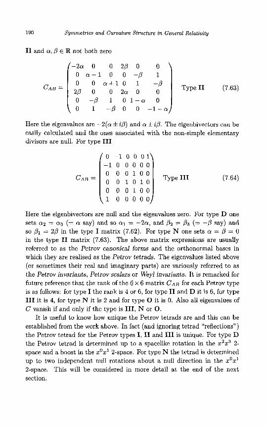
190 Symmetries and Curvature Structure in General Relativity
I1 and a,@ E IR not both zero
CAB =
-2a 0 0 2p 0 0 0 a - 1 0 0 -p 1 0 0 a + 1 0 1 -p 2p 0 0 2 0 0 0 0 -p 1 0 1 - a 0 0 1 -p 0 0 -1-a
Type I1 (7.63)
Here the eigenvalues are -2(a f ip) and a f $3. The eigenbivectors can be easily calculated and the ones associated with the non-simple elementary divisors are null. For type 111
CAB =
0 -1 0 0 0 1 -1 0 0 0 0 0 0 0 0 1 0 0 0 0 1 0 1 0 0 0 0 1 0 0 1 0 0 0 0 0
Type 111 (7.64)
Here the eigenbivectors are null and the eigenvalues zero. For type D one sets a2 = a3 (= a say) and so 011 = -2a, and = p 3 (= -p say) and so = 2p in the type I matrix (7.62). For type N one sets a = p = 0 in the type I1 matrix (7.63). The above matrix expressions are usually referred to as the Petrov canonical forms and the orthonormal bases in which they are realised as the Petrov tetrads. The eigenvalues listed above (or sometimes their real and imaginary parts) are variously referred to as the Petrov invariants, Petrov scalars or Weyl invariants. It is remarked for future reference that the rank of the 6 x 6 matrix CAB for each Petrov type is as follows: for type I the rank is 4 or 6, for type I1 and D it is 6, for type I11 it is 4, for type N it is 2 and for type 0 it is 0. Also all eigenvalues of C vanish if and only if the type is 111, N or 0.
It is useful to know how unique the Petrov tetrads are and this can be established from the work above. In fact (and ignoring tetrad “reflections”) the Petrov tetrad for the Petrov types I, I1 and 111 is unique. For type D the Petrov tetrad is determined up to a spacelike rotation in the z2z3 2- space and a boost in the zozl 2-space. For type N the tetrad is determined up to two independent null rotations about a null direction in the zozl 2-space. This will be considered in more detail at the end of the next section.

Space- Times and Algebraic Classification 191
7.4 Alternative Approaches to the Petrov Classification
So far, the Petrov Classification of the Weyl tensor has been described in terms of the latter’s eigenvector-eigenvalue structure. There are many other approaches and two of them, due to Be1 [65] (and Debever [66]) and Sachs [47], can now be described together. These result in a rather elegant approach to the Petrov canonical forms and the very useful Be1 criteria. + + + +
Recalling the self-dual property (*C = -iC) of C , one can write C = + + i (C + i*C) and so
Thus one may introduce the complex self-dual bivectors U , V and M from (7.33) to get
+ where A,. . . , F E C. Now the condition C a b a d = 0 is equivalent to C = E
above and so one achieves the elegant canonical decomposition of C in terms of the complex self-dual bivector basis U , V , M and C1,. . . , C5 E C given by Sachs [47]
+
+ C a b c d = C l v a b v c d + C 2 ( V a b M c d M a b V c d )
+ C 3 ( M a b M c d + VabUcd + U a b V c d ) -k c 4 ( u a b M c d + M a b u c d ) (7’67)
+ C 5 U a b U c d
To see how this relates to the Petrov classification one proceeds in a way similar to that used previously for bivectors. One performs null rotations about 1 given by (7.35) to see if the corresponding bivector transformations
(7.36) will yield a particularly simple “canonical” form for C in (7.66). Thus one imagines (7.67), but with primes on all quantities on the right hand side and then substitutes in (7.36). Equating back with the original
+
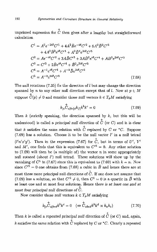
192 Symmetries and Curvature Structure in General Relativity
+ unprimed expression for C then gives after a lengthy but straightforward calculation
c1 = ~ 2 , - 2 i O c 1 1 + 4 ~ 2 B , - i O 12 c +6A2B2CI3 + 4 ~ 2 B 3 ~ i e ~ 1 4 + ~ 2 B 4 , 2 i B c i 5
c2 = ~ , - i e p + 3ABCl3 + 3 ~ ~ 2 , i e c 1 4 + ~ ~ 3 , 2 i e c t 5
c3 = c13 + 2 ~ e i e C ~ 4 + p e 2 i e c i 5
c4 = ~ - 1 ~ i O c 1 4 + ~ - 1 ~ ~ 2 i e ~ 1 5
c5 = ~ - 2 , 2 i 0 ~ 1 5 (7.68)
The null rotations (7.35) fix the direction of 1 but may change the direction spanned by n to any other null direction except that of 1. Now at p E M suppose C(p) # 0 and consider those null vectors k E T,M satisfying
+
+ k[eCa]bc [dkf ]kbkC = 0 (7.69)
Then k (strictly speaking, the direction spanned by k , but this will be
understood) is called a principal null direction of C (or C ) and it is clear
that k satisfies the same relation with C replaced by C or *C. Suppose (7.69) has a solution. Choose it to be the null vector 1’ in a null tetrad
( l ’ n ’dy ’ ) . Then in the expression (7.67) for C , but in terms of U’, V’ and MI, one finds that this is equivalent to CI5 = 0. Any other solution to (7.69) will then be (a multiple of) the vector n in some appropriately null rotated (about l’) null tetrad. These solutions will show up by the vanishing of C’ in (7.67) since this is equivalent to (7.69) with k = n. Now since CI5 = 0 one obtains from (7.68) a cubic in B and hence there are at
most three more principal null directions of C . If one does not assume that (7.69) has a solution, so that CI5 # 0, then C’ = 0 is a quartic in B with a t least one and at most four solutions. Hence there is a t least one and a t most four principal null directions of C .
+ +
+
+
+ Now consider those null vectors k E T,, M satisfying
+ + k[eCa~bcdkbkc = 0 (H Cabcdkbkd 0: kakc) (7.70)
Then k is called a repeated principal null direction of C (or C) and, again,
k satisfies the same relation with C replaced by C or *C. Clearly a repeated
+ +
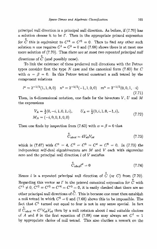
Space- Tames and Algebraic Classification 193
principal null direction is a principal null direction. As before, if (7.70) has a solution choose it to be 1'. Then in the appropriate primed expression
for C this is equivalent to Ct4 = Ct5 = 0. Then to find any other such solution n one requires C' = C2 = 0 and (7.68) shows there is at most one more solution of (7.70). Thus there are at most two repeated principal null
directions of C (and possibly none). To link the existence of these preferred null directions with the Petrov
types consider first the type I? case and the canonical form (7.63) for C with a = /3 = 0. In this Petrov tetrad construct a null tetrad by the component relations
+
+
l a = 2 - ll2 ( l , l , O , O ) na = 2-1/2(-1,1,0,0) ma = 2-1/2(0,0,1,-2) (7.71)
Then, in 6-dimensional notation, one finds for the bivectors V , U and M the expressions
V A = i(o,-i ,1,o,l , i) , U A = i(O,i,1,0,-1,2), (7.72) M A = ( - i , O , 0, 1,0, 0)
Then one finds by inspection from (7.63) with a = ,B = 0 that
(7.73)
which is (7.67) with C' = 4, C2 = C3 = C4 = C5 = 0. In (7.73) the independent self-dual eigenbivectors are M and V each with eigenvalue zero and the principal null direction 1 of V satisfies
+ Hence 1 is a repeated principal null direction of C (or C ) from (7.70).
Regarding this vector as 1' in the primed canonical expression for C with C'l # 0, CI2 = CI3 = CI4 = CI5 = 0, it is easily checked that there are no
other principal null directions of C. This is because one must then establish a null tetrad in which C1 = 0 and (7.68) shows this to be impossible. The fact that C' turned out equal to four is not in any sense special. In fact
if Cabcd = c l v a b v c d then by a null rotation about 1 and suitable choices of A and 0 in the first equation of (7.68) one may always set C1 = 1 by appropriate choice of null tetrad. This also clarifies a remark on the
+
+
+
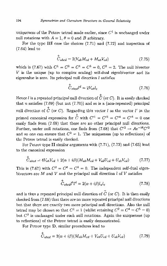
194 Symmetries and Curvature Structure an General Relativity
uniqueness of the Petrov tetrad made earlier, since C1 is unchanged under null rotations with A = 1, 0 = 0 and B arbitrary.
For the type I11 case the choices (7.71) and (7.72) and inspection of (7.64) lead to
+ Cabcd = 2 ( v a b M c d + M a b K d ) (7.75)
which is (7.67) with C1 = C3 = C4 = C5 = 0, C2 = 2. The null bivector V is the unique (up to complex scaling) self-dual eigenbivector and its eigenvalue is zero. Its principal null direction 1 satisfies
+ C a b c d l d = 2 v a b l c (7.76)
Hence 1 is a repeated principal null direction of C (or C). It is easily checked that n satisfies (7.69) (but not (7.70)) and so is a (non-repeated) principal
null direction of C (or C). Regarding this vector 1 as the vector 1' in the
primed canonical expression for C with C'l = Ct3 = Cr4 = CI5 = 0 one easily finds from (7.68) that there are no other principal null directions. F'urther, under null rotations, one finds from (7.68) that CI2 + Ae-ieC12 and so one can ensure that C2 = 1. The uniqueness (up to reflections) of the Petrov tetrad is easily checked.
For Petrov type I1 similar arguments with (7.71), (7.72) and (7.63) lead to the canonical expression
+
+ +
+ C a b c d = 4VabVcd + 2(a + '$)(MabMcd + V a b U c d + U a b V c d ) (7.77)
This is (7.67) with C2 = C4 = C5 = 0. The independent self-dual eigen- bivectors are M and V and the principal null direction 1 of V satisfies
+ C a b c d l b l d = 2((r + ' i P ) l a l c (7.78)
and is thus a repeated principal null direction of C (or C). It is then easily checked from (7.68) that there are no more repeated principal null directions but that there are exactly two more principal null directions. Also the null tetrad may be chosen so that C1 = 1 (whilst retaining C2 = C4 = C5 = 0) but C3 is unchanged under such null rotations. Again the uniqueness (up to reflections) of the Petrov tetrad is easily demonstrated.
+
For Petrov type D, similar procedures lead to + C a b c d = 2(a + i P ) ( M a b M c d + VabUcd + U a b x d ) (7.79)
Space- Tames and Algebraic Classification 195
which is (7.67) with C1 = C2 = C4 = C5 = 0. The independent self-dual eigenbivectors are M , U and V . Further 1 and n each satisfy (7.78) and
so each is a repeated principal null direction of C (or C). There are no other principal null directions. The coefficient C3 is unchanged under null rotations about 1 and the Petrov tetrad is determined up to null rotations about 1 with B = 0.
For Petrov type I the situation is a little more complicated. The proce- dures adopted so far, using (7.62), yield a canonical form
+
+ with C1 and C5 non-zero complex numbers (otherwise C would be type I1 or D) and which is (7.67) with C2 = C4 = 0. It follows from (7.68) that a null rotation about 1 may be employed so that in the new tetrad C1 = C5. An alternative form can be found by choosing 1 as a principal null direction (which necessarily exists) and hence C5 = 0. Now another principal null direction must exist. (If C1 = 0 it is spanned by n and if C1 # 0 the lack of another such null direction would necessitate C2 = C3 = C4 = 0 and imply that C is of type N, as follows from (7.68).) Building a null tetrad containing these principal null directions leads to (7.67) with C1 = C5 = 0 and the alternative form is
+
+ Cabcd = C 2 ( V a b M c d + M a b V c d ) + C 3 ( M a b M c d + VabUcd + UabVcd) (7.81)
f c 4 ( u a b M c d + M a b U c d )
where C2 and C4 are non-zero complex numbers. A computation of the self- dual eigenbivectors from either (7.80) with C1 = C5 or (7.81) is straight- forward. In the first of these expressions, for example, they are M and U f V .
Thus one achieves the canonical forms of Sachs [47] with those of Be1 [65] and Debever [66] following by taking the real parts of (7.73), (7.75), (7.77)
and (7.79). One can say a little more here. Suppose C admits a repeated principal null direction 1. Then in any null tetrad (1, n, IC, y) equation (7.67) shows that C4 = C5 = 0. Equation (7.68) then shows that, by a suitable null rotation, one can achieve exactly one of the expressions (7.73), (7.75), (7.77) or (7.79) for types N, 111, I1 or D, respectively. Thus if C is of type I it admits no repeated principal null directions. Then recalling the results established earlier, one sees that for Petrov type N there is a single
+
196 Symmetries and Curvature Structure in General Relativity
(necessarily repeated) principal null direction, for type I11 there are exactly two principal null directions, one repeated and one not, for type I1 there are exactly three principal null directions, one repeated and two not, for type D there are exactly two principal null directions, both repeated and for type I there are exactly four principal null directions, none of which is repeated. These were established above except for the existence of four distinct principal null directions in the type I case. This requires some algebra but follows more easily in the spinor approach due to Penrose [68].
It is usual to call the Petrov types 0, N, 111, I1 and D algebraically
special and the type I algebraically general. Thus C ( p ) (or C(P) ) is of an algebraically special Petrov type if and only if it admits a repeated princi- pal null direction. The repeated principal null directions in the type N and I11 cases are referred to, respectively, as quadruply and triply repeated and those in the type I1 and D cases as doubly repeated. Treating non-repeated principal null directions as single, one achieves a notion of “counting prop- erly” in which the “sum” of the principal null directions in each Petrov type is four. This can be given an algebraic meaning in the formalism developed here but is clearer in the spinor approach [68]. Repeated (respectively, non- repeated) principal null directions are often referred to as repeated (respec- tively, non-repeated) Debever-Penrose directions. This terminology, whilst appropriately recognising the work of Debever and Penrose, unfortunately fails to recall the work of Be1 (see reference [65] and earlier papers cited there).
The existence of repeated principal null directions through (7.70) im- plies that the Petrov type is algebraically special. However, it does not distinguish between those principal null directions which are doubly, triply or quadruply repeated. There exists a means of distinguishing such de- generacies and which links it to the Petrov classification. These features, essentially due to Be1 [65] are often referred to as the Be1 criteria.
Theorem 7.4 Then the condition that C ( p ) is of type N is equivalent to any of the following statements for some Ic E T,M, Ic # 0.
+
Let M be a space-time, p E M and C(p) # 0.
+ ( a ) C a b c d k d = 0 (b) C a b c d k d = 0 (c) * C a b c d k d = 0
+ (d) C a b l c d k z ] = 0 (e) C a b [ c d k ] = 0 (f) * C a b ( c d k e ] = 0
I n the conditions (a)-(’) k is necessarily null and unique up to scaling and spans the repeated principal null direction of C .
Space- T i m e s and Algebraic Classification 197
Proof. If C ( p ) is of type N then (7.74) shows that ( a ) holds. Also, dualling on the index pair ab shows that ( b ) @ ( c ) and clearly ( a ) ( b ) and (c ) and then ( b ) and (c) together imply ( a ) . Thus ( a ) , ( b ) and ( c ) are equivalent. Now for any tensor Ta. . .bcd at p , the condition Ta...bcdEbcde = 0, upon contraction with Eepqr , reveals that Ta. . . [bcd] = 0. So choosing Tabcde = C a b c d k e , condition (c) gives CabmnEmncdkd = o which implies ( e )
and clearly ( e ) @ (f). Then (e) or (f) * ( d ) and ( d ) gives * C a b [ c d k e ] = 0 and hence ( a ) holds. So ( a ) , . . . , (f) are equivalent and are implied by the type N condition. Conversely, if any (and hence all) of ( a ) , . . . , (f) hold, a contraction of (e) with k" and use of ( b ) shows that k is necessarily null. Essentially the same trick then shows that if ( a ) , . . . , (f) hold with k replaced by k' then k' is null and orthogonal to k. Thus the direction spanned by k is unique. Then choosing 1 = k in the expansion (7.67) for
C shows that only C1 does not vanish and reveals a type N expression like
+
+ (7.73). 0
Theorem 7.5 Let M be a space-time, p E M and C(p) not of type 0 o r N. Then the statement that C ( p ) is type 111 is equivalent to any of the following conditions for some k E T,M and some real bivector F at p with k and F non-zero.
+ ( a ) C a b c d k b k d = 0 ( b ) C a b c d k b k d = * C a b c d k b k d = 0
+ + ( C ) C a b c d k d = F a b k ( d ) C a b c d k d = F a b k c ( e ) * C a b c d k d = * F a b k c
The vector k and bivector F are null, unique up to scalings and k spans the repeated principal null directions of F and C(p) .
Proof. Clearly ( a ) H ( b ) and (c) H (d ) H (e) and any of these five conditions is implied by the type I11 condition expressed in (7.75). Now the second condition in ( b ) , together with a dualling argument similar to that used in the previous theorem, show that k a C a b [ c d k e ~ = 0. A contraction of this equation with ke (noting that kaCabcd # 0, otherwise c ( p ) would be type N) shows that k is null. Condition (u) and (7.67) with k replacing 1 then show that C2 # 0, C3 = C4 = C5 = 0 and then the use of a null rotation to get C1 = 0 recovers the type I11 expression (7.75). The uniqueness of k up to a scaling then follows. Finally, suppose ( c ) , ( d ) and ( e ) hold. Then a contraction of any of these conditions with k" shows that k is null and the condition C a b a d = 0 shows that F a b k b = * F a b k b = 0. Theorem 7.2 then shows that F is null with principal null direction k.

198 Symmetries and Curvature Structure in General Relativity
The uniqueness of F up to a scaling is now clear and (a) and (b) follow,
Theorem 7.6
completing the proof. 0
Let M be a space-time and let p E M .
i)
ii)
C(p ) is type I1 if and only if there exists a unique k E T,M, k # 0, such that
+ Cabcdkbkd = pk,k,
(or equivalently Cab,dkbkd = akak , and *Cabcdkbkd = @kakc) where p = a + ip # 0, a, p E R. The vector k is necessary null and spans the repeated principal null direction of C(p) . C(p ) is type D if and only if there exists two independent vectors k and k' E T,M satisfying the equation in part (a) above for non-zero complex numbers p and p'. It necessarily follows that p = p' and that k and k' are null and unique up to interchange and scalings and span the repeated principal null directions of C(p) .
Proof. The proof of this theorem has essentially been given in the pre- vious discussion. 0
It is convenient at this point to return briefly to the conditions (7.69) and (7.70) defining, respectively, a principal and a repeated principal null direction of the Weyl tensor at m E M . Provided it is given that k is null these conditions may each be replaced by the equivalent condition at m
obtained by replacing C by C or by C* +
k[eCa]bc[dkf]kbkc = 0 k [ e c z ] b ~ [ d k f ] k b k c = (7.82a)
k[,Ca]bcdkbkC = 0 k[,C,*]bcdkbkc = 0 (7.8213)
Then for k null the two conditions (7.82a) are equivalent to each other and to (7.69) and to the statement that k is a principal null direction of C. Similarly for k null the two conditions (7.82b) are equivalent to each other and to (7.70) and to the statement that k is a repeated principal null direction of C. These results can be checked from (7.67). It is remarked here that the first equation in (7.82b) implies that CabcdkbkC = ak,kd, a E R. If cu # 0 a contraction with k" shows that k is necessary null. Similar remarks apply to the second condition in (7.8213). Also in (7.82a) the first equation implies that CabcdkbkC = kaPd+Pakd for a covector P at m with P a k a = 0. A contraction with k a then reveals that if P # 0, k is necessary null. Similar remarks apply to the second condition in (7.82a). Thus in either (7.82a) or

Space- T imes and Algebraic Classification 199
(7.82b) the extra condition C,b,dkbkd # 0 or CZbcdkbkd # 0 forces k to be null and then either condition in (7.82a) (respectively, (7.82b)) forces k to span a principal (respectively, a repeated principal) null direction of C(p) .
The multiplicity properties of the principal null directions are conve- niently and traditionally represented for each Petrov type by the following self-explanatory (Penrose) diagram.
N D I
Fig. 7.1
It should be pointed out that the Petrov Classification is an algebraic statement about the Weyl tensor at p E M and the Petrov type may change if p changes. Some remarks about this will be made at the end of this chapter. If the Petrov type is the same at each p E M one refers to the space-time as being of that Petrov type.
Another important approach to the Petrov Classification is by using spinors. This approach, due to Penrose [68],[69], is rather elegant and is omitted here only because the tensor approach already discussed is more appropriate for the work in this book.
The canonical bivector decomposition given in this section allows the problem of the uniqueness of the Petrov tetrads to be reconsidered. Clearly the uniqueness or not of a frame where the Weyl tensor components assume a particular set of values can be established with any frame as starting point. The frames used in the above bivector decomposition are particularly
convenient. For example, suppose C(p) takes the type N form (7.73) with identical tetrad components in the null tetrads (1, n, x, y) and (1’, n’, x’, y’). Then 1‘ and 1 are proportional and these tetrads are thus related by a null rotation about 1 of the form (7.35). This rotation must be such that
the coefficient C’ of C(p) is unchanged. Thus one finds from (7.68) that and so A = 1, t9 = 0. Hence the allowed null rotations are
(7.35) with B arbitrary. For the Petrov type D a similar argument based on the canonical form (7.79) shows that any alternative real null tetrad must
+
+ ~1 = ~ 1 ~ 2 ~ - 2 i 9
200 Symmetries and Curvature Structure in General Relativity
have its real null members spanning the two (necessarily repeated) principal null directions of C(p) and that the coefficient C3 must be unchanged. Hence from (7.35) and (7.68) one finds B = 0. Hence the allowed null rotations are (7.35) with B = 0 and A and 8 arbitrary. Similarly arguments for the Petrov types 11, I11 and I yield A = 1, 8 = 0, B = 0 and so in this sense and for these types the tetrad is uniquely determined.
Another point of interest concerns the relationship between the or- thonormal Petrov tetrads in which the canonical Petrov forms (7.62), (7.63) and (7.64) are described and the (repeated and non-repeated) principal null directions of the Weyl tensor at m E M . If the Petrov type at m is N, I11 or D one has the canonical forms given in (7.73), (7.75) and (7.79) and in these complex null tetrads (1, n, m, m), 1 (for type N) and 1 and n for types I11 and D are the (only) principal null directions. In each case it is easily checked that ( t , xl, x2, x3) is a Petrov tetrad where f i t = 1 - n, fix’ = 1 + n and f i m = x2 + ix3. However, the link between the Petrov tetrads and the principal null directions is less obvious for Petrov types I and 11. The problem for the type I case was considered in [70] and here both types will be dealt with by a slightly different method. If C is of Petrov type I1 at m, the canonical form (7.77) applies and the Petrov tetrad is obtained from the complex null tetrad just as for the types N, I11 and D above. Now although 1 is the repeated principal null direction of C at m, the null vector n in the tetrad spans neither of the remaining principal null directions of C. Now perform two null rotations using (7.35) each on the above original complex null tetrad (1, n, m, f i ) (the original tetrad chosen so that C” = 1 in (7.67)) with A = 1, 8 = 0 and B = fF, F = i(6C’3)-1’2. The null vector n is transformed, respectively, to n1 and n2 where
n1 = n - IFI21 + p 722 = n - IFI21 - p (7.83)
and where p = F m + F f i is a real spacelike vector lying in the x2x3 2- space. It can then be checked that n1 and 722 span (non-repeated) principal null directions of C since in each of these new tetrads, C1 = 0. Now put r = n - IFI21 so that r is timelike and orthogonal to p. Then n1 = r +p , n2 = r - p (+ 27 = n1 + n2, 2p = n1 - n2) and so the direction of r is fixed by the intersection of the timelike 2-spaces spanned by 1 and n and by n1 and 122. This enables figure 7.4 to be constructed and which shows the relation between the canonical null tetrad (1, n, m, 6) (or its associated Petrov tetrad ( I , n, z2, x3) given above) and the principal null directions 1, n1 and 712.
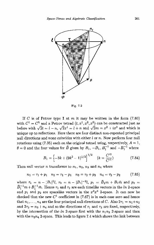
Space- Tames and Algebraic Classaficataon 201
c n
Fig. 7.2
If C is of Petrov type I at m it may be written in the form (7.80) with C' = C5 and a Petrov tetrad ( t , x l , x 2 , x 3 ) can be constructed just as before with f i t = 1 - n, f i x 1 = 1 + n and f i m = x2 + ax3 and which is unique up to reflections. Here there are four distinct non-repeated principal null directions and none coincides with either 1 or n. Now perform four null rotations using (7.35) each on the original tetrad using, respectively, A = 1, 6 = 0 and the four values for B given by B1, -B1, B;' and -B;' where
112 Ct3 C'1 B1 = [ -3k + (9k2 - 1)'/2] (k = -) (7.84)
Then null vector n transforms to nl, n2, n3 and 124 where
n1 = 71 + p l n2 = 71 - p l ng = 72 + p2 724 = 72 - p2 (7.85)
where 71 = n - IB1I2Z, 7 2 = n - IB11-2Z, p l = Blm + B1fi and p2 =
B;'m+ BF1fi. Hence 71 and 72 are each timelike vectors in the In 2-space and p l and p2 are spacelike vectors in the x2x3 2-space. It can now be checked that the new C1 coefficient in (7.67) is in each case zero and hence that nl, . . . ,724 are the four principal null directions of C. Also 271 = nl+n2 and 272 = 723 + 124 and so the directions of 71 and 72 are fixed, respectively, by the intersection of the In 2-space first with the 721122 2-space and then with the 723724 2-space. This leads to figure 7.4 which shows the link between
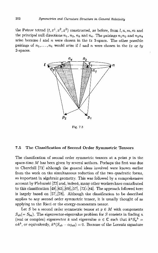
202 Symmetries and Curvature Structure in General Relativity
the Petrov tetrad (t , x l , x2 , x3 ) constructed, as before, from 1, n, rn, iiz. and the principal null directions n l , n 2 , n3 and 724. The pairings 7x1722 and n 3 n 4
arise because 1 and n were chosen in the t z 2-space. The other possible pairings of 7 2 1 , . . . , n 4 would arise if 1 and n were chosen in the t x or t y 2-spaces.
P2 Pl
Fig. 7.3
7.5 The Classification of Second Order Symmetric Tensors
The classification of second order symmetric tensors at a point p in the space-time M has been given by several authors. Perhaps the first was due to Churchill [71] although the general ideas involved were known earlier from the work on the simultaneous reduction of the two quadratic forms, so important in algebraic geometry. This was followed by a comprehensive account by Plebanski [72] and, indeed, many other workers have contributed to this classification [48], [63], [69], [57], [73]- (841. The approach followed here is largely based on [57],[78]. Although the classification to be described applies to any second order symmetric tensor, it is usually thought of as applying to the Ricci or the energy-momentum tensor.
Let S be a second order symmetric tensor at p E M with components &b(= &,a). The eigenvector-eigenvalue problem for s consists in finding a (real or complex) eigenvector k and eigenvalue Q E C such that kaSab = a k b , or equivalently, ka(Sab - Qgab) = 0. Because of the Lorentz signature
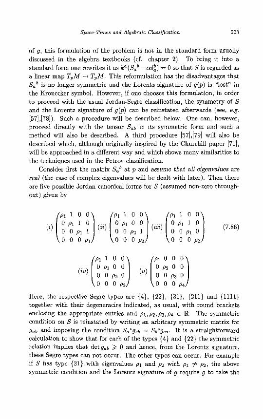
Space- Tames and Algebraic Classification 203
of g, this formulation of the problem is not in the standard form usually discussed in the algebra textbooks (cf. To bring it into a standard form one rewrites it as ka(Sab - a6:) = 0 so that S is regarded as a linear map T,M --+ T,M. This reformulation has the disadvantages that Sab is no longer symmetric and the Lorentz signature of g(p) is “lost” in the Kronecker symbol. However, if one chooses this formulation, in order to proceed with the usual Jordan-Segre classification, the symmetry of S and the Lorentz signature of g(p) can be reinstated afterwards (see, e.g. [57],[78]). Such a procedure will be described below. One can, however, proceed directly with the tensor S a b in its symmetric form and such a method will also be described. A third procedure [57],[79] will also be described which, although originally inspired by the Churchill paper [71], will be approached in a different way and which shows many similarities to the techniques used in the Petrov classification.
Consider first the matrix Sab at p and assume that all eigenvalues are real (the case of complex eigenvalues will be dealt with later). Then there are five possible Jordan canonical forms for S (assumed non-zero through- out) given by
chapter 2).
Here, the respective Segre types are {4), {22), (31}, (211) and (1111) together with their degeneracies indicated, as usual, with round brackets enclosing the appropriate entries and pl,p2,p3,p4 E R. The symmetric condition on S is reinstated by writing an arbitrary symmetric matrix for gab and imposing the condition SaCgcb = It is a straightforward calculation to show that for each of the types (4) and (22) the symmetric relation implies that detgab 3 0 and hence, from the Lorentz signature, these Segre types can not occur. The other types can occur. For example if S has type (31) with eigenvalues p1 and p2 with p1 # p2, the above symmetric condition and the Lorentz signature of g require g to take the
204 Symmetries and Curvature Structure in General Relativity
form gab with 912 = 913 = 922 = 923 = 903 = 0, 911 = 902 and with 902 > 0 and 933 > 0 in the corresponding Jordan basis at p (the only other possibility 902 < 0 and 933 < 0 gives signature (+, -, -, -)). In this basis, eigenvectors may be chosen as 1" 3 (0, 0,1,0) with eigenvalue p1 and ya = ( O , O , 0 , l ) with eigenvalue p2. It then follows that la la = laya = 0 and yaya > 0. A null tetrad can then be built around 1 and y' =
and a general expression for S constructed in this tetrad which may then be simplified by the use of the null rotations (7.35) about 1. By this procedure one can construct canonical expressions for each of the remaining types (7.86) (further details may be found in [57]). However, one would still have to deal with the case when the eigenvalues are not all real and for this and other reasons a different approach will be used to obtain these canonical forms for S. This alternative approach deals directly with the symmetric tensor Sat, and has the Lorentz signature built into it from the outset. Also, the case when the eigenvalues are not all real poses no problems. This involves a brief digression into the invariant 2-space structure of S.
A 2-space W 5 T,M is called an invariant 2-space of S at p if, whenever ua is in W , so also is uaSab. Now if S has all eigenvalues real at p it takes one of the Jordan types (7.86) and in such a basis the last two members of that basis span an invariant 2-space of S at p . If, on the other hand, S has a non-real eigenvector w at p , the real and imaginary parts of w span an invariant 2-space of S at p (section 2.6). Hence S always admits an invariant 2-space at any p E M and the following theorem records some of their properties (cfthe comments on invariant 2-spaces of bivectors at the end of section 7.2).
Theorem 7.7 second order symmetric tensor at p . Then at p
Let M be a space-time, let p E M and let S # 0 be a
a) i f W is an invariant 2-space of S so also is its orthogonal complement, i i) S admits a null invariant 2-space W if and only if S admits a real null
eigenvector w (and w may be chosen in W) , iii) S admits a spacelike (equivalently, f rom (i), a timelike) invariant 2-
space i f and only if S admits an orthogonal pair of spacelike eigenvectors (which necessarily lie in the spacelike invariant 2-space).
Proof. It is useful here and elsewhere to note the decomposition of S
Space- Times and Algebraic Classification 205
along a real null tetrad (1, n, x, v) at p. This is
where S1, ..., S I O E R. Such an expression for S a b may be simplified by null rotations (say, about 1) using the equations (7.35) written out in their real and imaginary parts so as to apply to the (real) null tetrad (1, n , x, y) with d m = x+iy. The procedure is essentially the same as that used to obtain (7.68) for the Weyl tensor and will prove useful in what is to follow. (i) Suppose that W is spacelike and taken to be spanned by x and y. Then it follows from (7.87) that S4 = S5 = S6 = S7 = 0 and then that 1 and n (which span the orthogonal complement of W ) also span an invariant 2- space of S. If W is timelike one merely reverses the argument. If W is null and taken to be spanned by 1 and x then one finds S3 = S6 = S7 = S8 = 0 and so 1 and y span an invariant 2-space of S (and is again the orthogonal complement of W ) . It also follows that 1 is a null eigenvector of S. (ii) If W is a null invariant 2-space of S then the last sentence of (i) above confirms the existence of a null eigenvector of S. Conversely if S admits a null eigenvector, taken as 1, then (7.87) show that S3 = S6 = S7 = 0. A null rotation (7.35) with A = 1 and B = 0 can then be used (if necessary) to form a new null tetrad in which S8 = 0 also. Then, in this new tetrad, 1 and x span a null invariant 2-space of S. (iii) If W is a spacelike invariant 2-space of S spanned, say, by x and y then (7.87) holds with S4 = S5 = S6 = S7 = 0. A null rotation (7.35) with A = 1 and B = 0 can again be used to set S8 = 0 also and then x and y are eigenvectors of S. Conversely, if x and y are taken as the orthogonal pair of spacelike eigenvectors of S then (7.87) gives S4 = S5 = S6 = S7 = S8 = 0 and the result is clear. 0
The theorem which gives the complete algebraic description of S at p can now be given.
Theorem 7.8 second order symmetric tensor at p .
Let M be a space-time, let p E M and let S # 0 be a Then S takes one of the following
206 Symmetries and Curvature Strzlcture in General Relativity
canonical f o r m s in t e r m s of s o m e (real) nu l l tetrad ( I , n, x , y ) a t p .
S a b = 2p l l (anb) + P2(lalb f n a n b ) f p3xaxb -k P4YaYb Sab = 2p l l (anb) -k Xlalb + p2xaxb + P3YaYb S a b = 2p l l (anb) + 21(axb) + p l x a x b f P2YaYb S a b = 2p l l (anb) + P2(lalb - n a n b ) -k p3xaxb + P4YaYb
(7.88a)
(7.88b)
(7 .88~)
(7.88d)
where all p i E R and where O#XER in (7.88b) and p2 # 0 in (7.88d). In ( 7 . 8 8 ~ ) ~ t h e eigenvectors can be t a k e n as t = 2-1/2(1 - n) (with eigenvalue p i - P Z ) , z = 2-l l2(1 + n) (PI + p2) , x (p3) and y ( ~ 4 ) . T h e eigenvector t is t imel ike and x , y and z are spacelike and ( t , x , y, 2) is a n orthonormal tetrad. T h e Segre type is {1,111} or o n e of i ts degeneracies. (In this type, a c o m m a will be used t o separate t h e eigenvalue arising f r o m a t imel ike eigenvector f r o m those arising f r o m spacelike eigenvectors. T h i s will be ex- plained in m o r e detail later.) T h u s S is diagonalisable over R. In (7,88b), t h e eigenvectors m a y be t a k e n as l ( p l ) , x ( p 2 ) and y ( p 3 ) and, wi thout affect- i ng the remainder of (7.88b), t h e nu l l tetrad m a y be chosen so tha t X = 1 ( i f X > 0 ) and X = -1 (if X < 0). T h e Segre type is ( 2 1 1 ) or o n e of its degeneracies. In ( 7 . 8 8 ~ ) ~ t h e eigenvectors m a y be t a k e n as l ( p 1 ) and y ( p 2 ) and t h e Segre t ype i s (31) or one of i t s degeneracies. T h e case (7.88d) i s t h e only case where non-real eigenvectors occur and t h e y m a y be t a k e n as 1 f i n ( p 1 f i p z ) , t h e other eigenvectors being t a k e n as x ( p 3 ) and y ( p 4 ) . T h e Segre type i s {zZll) or i t s degeneracy. An alternative f r o m for (7 .88~) i s
Sab = (p2 - P l ) t a t b + ( p l + p2)zazb + P3xaxb + P4yaYb (7.88e)
Proof. First it should be pointed out that the description of the eigen- vectors and eigenvalues in (7.88a) to (7.88d) can easily be checked. The statements regarding the Segre types of these canonical expressions for S then follow from the number of independent eigenvectors and the fact that only the above mentioned four Segre types are possible. Two general cases will be considered; when S admits a real null eigenvector and when it does not.
If S admits such a null eigenvector 1, construct a null tetrad (1,n, x , y ) so that S decomposes as in (7.87) with S 3 = S6 = S7 = 0. Then a null rotation (7.35) with A = 1 and B = 0 can be used to preserve these conditions and to achieve, in addition, S8 = 0. Now four possibilities arise concerning the coefficients S1, S9 and SIO.
(a) S9 # S1 # S I O . A null rotation with A = 1 and 0 = 0 can be used to obtain a new tetrad in which S3 = S4 = S5 = S6 = S7 = Ss = 0 and
Space-Times and Algebraic Classification 207
hence S takes the form (7.88b) but with S2 possibly zero. If S2 # 0 the Segre type is thus (211) or {2(11)} (the latter occurring if S9 = Sl0). If S2 = 0, equation (7.88a) can now be used to see that the Segre type is
(b) S1 = S9 # S I O . If also S4 = 0 then one has S3 = S4 = S6 = S7 = 0 and a null rotation with A = 1 and 8 = 0 can be used to obtain an expression like (7.8813) again and so the Segre type is {(21)1) or ((1,ll)l) depending on whether S2 # 0 or S2 = 0. If, however, S4 # 0 in the original tetrad a null rotation with A = 1 and 8 = 0 can be used to obtain a tetrad in which S2 = S3 = S5 = S6 = S7 = S8 = 0 and so an expression like (7.88~) results. A null rotation can then be used to set Rd = 1. The Segre type is
(c) S1 = S I O # S9. This case is essentially the same as the last one. (d) S1 = S9 = SIO. Here, the same techniques as above show that
if S4 = S5 = 0 in the original tetrad, then one arrives at the Segre type ((211)) or {(1,111)}. If, however S4 and S5 are not both zero a null rotation can be used to cast S into the Segre type ((31)) canonical form.
Now suppose that S has no real null eigenvectors. Then from theorem 7.7(ii) S admits no null invariant 2-space. Since S must admit some in- variant 2-space W , W must be spacelike or timelike and hence (theorem 7.7(iii)) S admits an orthogonal pair of (unit) spacelike eigenvectors, say z and y . On constructing a null tetrad (1, n, 2, y ) around z and y , it then follows that S takes the form (7.87) with S4 = S5 = S6 = S7 = S8 = 0 and with S2 # 0 # S3 (otherwise real null eigenvectors would be admitted). A null rotation with 8 = B = 0 can then be used to arrange that IS2] = IS3/. The two possibilities S2 = S3 and S2 = -S3 lead, respectively, to (7.88a) with p2 # 0 and p3 # p1 - p2 # p4 and to (7.88d) with p2 # 0. These are the Segre types {1,111}, {1,1(11)) or {1,(111)} in the first case and { t Z l l ) or (zZ(l1)) in the second.
The remark in the statement of the theorem about being able to choose X = f l in (7.88b) follows by performing a null rotation with 8 = B = 0
{(1,1)11) or {(1,1)(11)).
(311.
and choosing A accordingly. 0
There are some other simple algebraic properties of a second order sym- metric tensor S that can now be collected together.
Theorem 7.9 second order symmetric tensor at p .
Let M be a space-time, let p E M and let S # 0 be a
i ) S admits at least two independent real eigenvectors, which m a y be cho-
208 Symmetries and Curvature Structure in General Relativity
sen orthogonal, and at least one of them is spacelike. i i) S admits a (real) timelike eigenvector i f and only i f it is of Segre type
(1,111) or one of its degeneracies (equivalently S is diagonalisable over
iii) S admits two (or more) independent (real) null eigenvectors if and only if it admits two (or more) independent (real) timelike eigenvectors (and if such is the case each of these null and timelike eigenvectors have the same eigenvalue). These conditions are equivalent to the statement that S has Segre type ((1,l)ll) or one of its degeneracies.
iv) S has all its eigenvalues real but possesses non-simple elementary divi- sors (i.e. it has Segre type (211) or (31) or one of their degeneracies) if and only i f S has a unique (real) null eigendirection (which then corresponds to the non-simple elementary divisor).
w.
Proof. the eigenvectors which exist for each canonical form (7.88a)-(7.88e).
The proofs of each part can essentially be obtained by a study of 0
It is useful here to note that if S admits eigenvectors u and v with distinct eigenvalues then u and v must be orthogonal as follows easily by contracting the equations Sab’ub = plua and S a b V b = P2Va ( p 1 # p 2 ) with va and ua, respectively, and using the symmetry of S. The results in (ii) and (iii) above show that only in the Segre type {l,lll}, or one of its degeneracies, can timelike eigenvectors occur and that a unique eigenvalue is associated with them. This “timelike eigenvalue” is indicated as the first digit in the Segre symbol and separated from the others by a comma (as mentioned, without justification, earlier).
7.6 The Anti-Self Dual Representation of Second Order Symmetric Tensors
A study of the algebraic structure of a second order symmetric tensor such as S above using its invariant 2-space structure was first considered by Churchill [71]. Here this idea will be taken up in a different way and which exhibits some similarities with the Petrov classification of the Weyl ten- sor [57],[79]. One notes here that the eigenvectors, Segre type (including degeneracies) and invariant 2-space structure (but, in general, not the eigen- values) of S are identical to those of the tracefree part of S , denoted by
Space- Times and Algebraic Classif ication 209
and defined by
(7.89)
To consider this approach to the classification of S , define a (0,4) tensor
1 S a b = S a b - ; i ( s c c ) g a b (* see = 0)
P at p E M by
Pabcd = saa[cgd]b + s b [ d g c ] a (* P C a c b = S a b ) (7.90)
Then P satisfies the following symmetry relations (in which the bracketed result follows from (7.49))
Pabcd = -Pbacd = -Pabdc Pabcd = Pcdab (7.91)
Pa[bcd] = 0 (e p a * b a d = 0) (7.92)
Thus P is the same type of tensor studied at the beginning of section 7.3 and so the Ruse-Lanczos identity (7.47) together with (7.90) give * P* + P = 2P and hence
*Pabcd = Pabcd (e *Pabcd = -Pabed) (7.93)
F’rom the definition (7.90) of P one finds
Thus if one regards the definition of P as that of a linear map f from the 9-dimensional vector space of tracefree second order symmetric tensors at p into the vector space of type (0,4) tensor at p then (7.94) shows this map to be one-to-one and thus the type (0,4) tensors in the range o f f (i.e of the form (7.90)) are, in this sense, “characteristic” of such second order symmetric tensors. Further, because of the conditions (7.93), P is called
anti self-dual. Now one may define a complex tensor P associated with P (and noting that, unlike the analogous situation with the Weyl tensor, the position of the dual symbol is important)
+
(7.95)
which satisfies the first set of symmetry properties in (7.43) but not the second since now, using a similar argument - to that given for Weyl tensor,
one has P&d = -P:dab and hence Pabcd = P c d a b . One also has the relations + +

210 Symmetries and Curvature Structure in General Relativity
+ + + + +
and the result that P = 0
s. Then
Pabad = S b d (from (7.90) and (7.92)), P:bcd = -iPabcd, 'Pabcd = iPabcd + = 0.
NOW let U C T,M be an invariant 2-space of spanned, say, by T and
(0, P, 71 6 E q (7.96)
Now the set of all simple bivectors whose blade is U is just the set of non- zero real multiples of the (real) bivector Fab = 2r [ ,Sb] and this statement is independent of the representative bivector F chosen. Then it follows that (7.96) is equivalent to
- b SabS = 7 T a + 6Sa SabTb = (Yra + P S a ,
Sb[aFbc] = pFac ( P E R) (7.97)
where p is independent of the representative bivector F. This condition, with the help of (7.90) and (7.95), can be written in the following three equivalent ways
+ + (i) PabcdFCd = 2pFab (iii) PabcdFCd = 4ppab
(7.98)
where F and fi are as in (7.20). Thus an invariant 2-space U of S (equiv- alently, of S ) determines up to a real multiple a real simple eigenbivector F of P and, conversely, a real simple eigenbivector F of P determines a unique invariant 2-space of S (or S ) and, in fact, is the blade of F. Also (7.98) shows that such eigenbivectors of P come in dual pairs, reflecting the fact that invariant 2-spaces of S (or S) come in orthogonal pairs (theorem 7.7) and, of course, the blades of a simple bivector and its dual are or- thogonal. Thus the invariant 2-space problem for S become one of finding simple (real) eigenbivectors of P. But if F is any (real) eigenbivector of P satisfying (7.98(i)) then a contraction with *Fab gives, using (7.93)
(ii) Pabcd*FCd = -2p*Fab
+
2pFab(*Fab) = Pabcd(*FabFcd) = *PabcdFabFcd = -P,6cdFabFCd (7.99) - - -PabcdFab*FCd = -PcdabFab*Fcd = -2pFab(*Fab)
and so, if p # 0, Fab*Fab = 0 , which, from theorem 7.1, is equivalent to F being simple. If p = 0 then F and ' F are eigenbivectors of P with zero eigenvalue and then some duality rotation of F (section 7.2) yields a real simple eigenbivector of P with zero eigenvalue. In this sense, the invariant 2-space problem for (or S ) becomes that of finding (real) simple eigenbivectors of P . But now suppose (7.98)(iii) holds for p E C and some
Space- Times and Algebraic Classif ication 211
+ + complex self-dual bivector F = F + i*F. Then a duality rotation F + + + + H = eieF reveals a complex self-dual bivector H satisfying (7.98(iii)) with
p E R for appropriate e E R. This follows since P a b c d H C d = 4 / L e 2 i e H a b . It is now easily checked that (7.98)(i) and (ii) hold for the real and imaginary
parts H and * H of H (and p E R). Thus the invariant 2-space problem for 3 (or S ) becomes that of solving (7.98(iii)) for p E R.
The solution of this last problem proceeds on similar lines to that for
+ +
+
the tensor C. One first chooses a complex null tetrad (1, n, m, a), then the complex self-dual bivectors U , V and M as in (7.24)-(7.26) and then
decomposes P as follows [57],[79] (cf(7.65)). +
Then by using (7.33) and its conjugate one has
+ Pabcd = P l U a b U c d -k P2VabVcd -k P 3 M a b M c d + P4UabVcd (7.101)
+ P5VabUcd + P 6 U a b M c d -k P 7 M a b U c d f P 8 V a b M c d + P S M a b V c d
- + + where PI , ..., PS E (C and where the condition Pabcd = P c d a b reveals that P I , P 2 , P 3 E R and that Ps = p4, P 7 = PG and Pg = &. The classification + is now based on the number of independent complex self-dual solutions F of (7.98(iii)) and their type (null or non-null). From the resulting canonical
expressions, S and hence S , are recovered from the contraction Sbd = p a b a d .
It is remarked here that this problem is similar to that encountered in the Petrov classification. Using the abbreviated notation employed in sec-
tion 7.3, the tensors P and P give rise to linear maps CB(p) -+ CB(p) which, using ideas very similar to those for the Weyl tensor, have the prop-
+
+
erties that P maps S+(p) -+ S-(p) and S-(p) -+ S+(p) and that k maps
S+(p) -+ S-(p) and S-(p) + 0 (and that for F E S+(p) , PF = 2PF) . there is always a non-
+ + Since there is always an invariant 2-space of
212 Symmetries and Curvature Structure in General Relativity
+ trivial F satisfying (7.98(iii)). Hence this latter equation has either one, two or three independent solutions in the complex 3-dimensional vector space of complex self-dual bivectors. Now if there are two independent null solutions then it is easy to see that a complex null tetrad (Z,n,m,m) may be chosen so that these solutions may be taken as U and V in (7.98(iii)). But (7.101) then reveals that PI = Pz = P6 = P7 = Ps = Pg = 0 and hence that M is a (non-null) solution. On the other hand if no null independent solutions of (7.98(iii)) exist then there exists a non-null solution, which may be taken as M , and so (7.101) gives P6 = P7 = Pa = Pg = 0. But one must also have PI # 0 and P2 # 0 (to avoid U or V becoming null solutions). A null rotation (7.35) with B = 0 can then be used to preserve the restrictions achieved so far and to obtain, in addition, lP1l = lPzl and P4 E R. If PI = P2 then U f V become extra independent non-null solutions of (7.98(iii)) whilst if PI = -P2 it can be checked that M is the only solution. The separate cases can now be discussed and the techniques required to obtain the canonical forms are very similar to those above and to those used in the Petrov classification. Hence the details are omitted but can be found in [57],[79] (cf.[72]).
Case(i) Suppose there is one independent solution to (7.98(iii)) and it is non-null. Choosing it as M one may arrange the tetrad (1, n, m, 752) SO
that
where PI, P3, P4 E R and PI # 0. A contraction of this yields the canonical form (7.88d) for s a b and hence the Segre type {zZll} or its degeneracy.
Case(ii) Suppose there is one independent solution to (7.98(iii)) and it is null. Choosing it as V one may arrange the tetrad so that
+ Pabcd = & ( f i a b M c d -2UabKd-2VabUcd) + P.(VabMcd + MabVcd) (7.103)
where P3, Ps E R and Ps # 0. A contraction of this leads to (7.88~) and the Segre type (31) or its degeneracy.
Case(iii) Suppose there are exactly two independent solutions of (7.98(iii)). Then the remarks above show that they may be taken as a null solution and a non-null solution and, in a suitable tetrad, as V and M , respectively. Then
+ Pabcd = p 2 V a b K d + P3MabMcd + P 4 ( 0 a b V c d -k VabUcd) (7.104)
Space- T i m e s and Algebraic Classification 213
with P2, P3, P4 E R and P2 # 0. A contraction then leads to (7.88b) and the Segre type (211) or one of its degeneracies.
Case(iv) Suppose there are three independent solutions to (7.98(iii)). If there are no null solutions the tetrad may be chosen so that
+ Pabcd = Pl(UabUcd + V a b V c d ) + P3MabMcd -k P4(UabVcd f V a b U c d ) (7.105)
with PI , P3, P4 E R (together with certain further restrictions on these coefficients to prevent null solutions). A contraction then reveals (7.88a) and the Segre type (1,111) together with the degeneracies permitted by these coefficient restrictions and which are p2 # 0, p3 # p1 - p2 # p4.
The only other possibility is that there are a t least two independent null solutions of (7.98(iii)). Then the tetrad may be chosen so that
+ Pabcd = P3MabMcd + P4(UabVcd + V a b U c d ) (7.106)
with P3, P4 E R and the usual contraction leads to (7.88a) with p2 = 0 and hence to the Segre type ((1,l)ll) or one of its degeneracies. This completes the classification.
The similarity of the classification of the second order symmetric tensor S (though the tensor P ) with the Petrov classification can be extended by linking the algebraic types of S with certain null directions which play
a similar role with respect to P (and P ) that the null directions of Bel,
Debever and Penrose play with respect to the Weyl tensor C (and C). The next theorem, whose proof will be omitted since it is similar to proofs given in the Weyl tensor case, summarises the situation.
Theorem 7.10
tensor at p with associated (O,4) tensor P.
+ +
Let M be a space-time, p E M and S # 0 a second order symmetric
i ) The statement that S has Segre type ((211)) is equivalent to any of the following statements for some k E T,M, k # 0
d + ( a ) Pabcdkd = 0 ( b ) Pabcdkd = 0 ( C ) Pzbcdk = 0
+ ( d ) P a b [ c d k e ] = 0 ( e ) Pab[cdke] = o (f) p$,[~dke] = o
In the conditions (a)-('), k is necessarily null and unique up to a scaling and spans the (unique) real null eigendirection of S . Each of these
214 Symmetries and Curvature Structure an General Relativity
+ conditions is equivalent to P taking the form (7.101) with 1 = k and Pz the only non-vanishing coefficient, and also to s a b = p2kakb.
i i) The statement that S has Segre type ((31)) is equivalent to any of the following statements f o r some k E T p M , k # 0 and some real null bivector F # 0.
+ + (a) kaPabcd = kbFcd, (b) kaPabcd = kbFcdr
I n these conditions k is necessarily null, and unique up to a real scaling and spans the (unique) real null eigendirection of S and the (unique) principal null direction of F . Each of these conditions is equivalent to
P taking the form (7.101) with 1 = k and P2, Pg and Pg the only non- vanishing coeficients (and then P2 can be set to zero by means of a null rotation) and also to &, taking the form ( 7 . 8 8 ~ ) with p1 = p2 = 0.
iii) The statement that a null vector k E TpM is an eigenvector of S with eigenvalue -p is equivalent to any of the following (equivalent) condi- tions (with p E W)
( C ) kaP&d = kb*Fcd
+
+ (a ) kakcPabcd = pkbkd (b) kakcPabcd = Pkbkd
( C ) kakCP,bcd = 0.
iv) The statement that a null vector k E T p M satisfies Sabkakb = 0 (equiv- alently Sabkakb = 0) is equivalent to any of the following (equivalent) conditions.
(c) k[epGb~[dkf]kbkc = O.
Part (iii) of this theorem shows how, what might be termed a “repeated
principal null direction” of P (or P ) , coincides with a null eigendirection of S and vice-versa. Part (iv) indicates the relevance to S of a “principal
null direction” of P (or P ) . Theorem 7.10 describes what might be termed
generalised Be1 criteria for P (or P ) or S. However, there are some differ- ences due to the anti self-dual nature of P. For example, the number of distinct real null directions satisfying the conditions in either (iii) or (iv) of the ahove theorem could be none, finitely many or infinitely many. (cfthe
+
+ +
Space- T i m e s and Algebraic Classification 215
case for the Weyl tensor where the respective numbers are 0, 1 or 2 and 1,2,3 or 4) [85].
There are several other approaches to the classification of second order symmetric tensors. Of particular interest is the approach due to Penrose [76] who classifies such a tensor by the type of curve on a complex quadric surface to which it corresponds. The relation between Penrose’s approach and the present one has been given [81],[85]. A spinor approach is also
available [72],[8O] and is closely related to the approach using the tensor P given above. A direct 6 x 6 classification of the tensor P can also be used and which, because of the symmetries of P, is quite straightforward [81].
+
7.7 Examples and Applications
The Ricci and energy-momentum tensor of space-time are second order symmetric tensors at any p E M and are hence subject to the procedures of the last two sections. The fourth order tensor arising from the Ricci tensor according to (7.90) is easily seen from (7.11) to be the tensor E. Then (7.10) can be viewed as a decomposition of the curvature at p E M into its self-dual and anti self-dual parts because
The energy-momentum tensor T has also been subjected to the domi- nant energy conditions (7.9) that for any p E M and any timelike or null u E T,M (i) Tabuaub 2 0 and (ii) Tabub is not spacelike. These condi- tions place restrictions on the Segre type of T at each p E M (see e.g. 1721 1 [481 , 1571 Theorem 7.11 momentum tensor at p .
Let M be a space-time, p E M and let T be the energy-
i ) I f the energy conditions are satisfied T cannot be of Segre type {zZll) or (31) or any of their degeneracies. ( In fact, i f T is of either of these types it cannot satisfy any of the conditions (a) and (ii) above.)
ii) If T has Segre type (211) o r one of its degeneracies (equation (7.88b)) the energy conditions are satisfied i f and only i f X > 0, p1 I 0, P1 I P2 I -P1 and p1 I p3 I -p1.
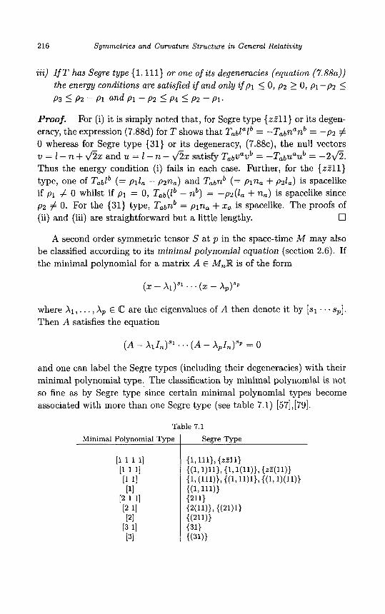
216 Symmetries and Curvature Structure in General Relativity
iii) If T has Segre type (1,111) or one of its degeneracies (equation (7.88a)) the energy conditions are satisfied if and only if p1 5 0 , p2 2 0, p 1 - p ~ 5 P3 5 P2 - P1 andp1 - P 2 I P4 I P2 -p1.
Proof. For (i) it is simply noted that, for Segre type (zZ11) or its degen- eracy, the expression (7.88d) for T shows that TabZalb = -Tabnanb = -p2 # 0 whereas for Segre type (31) or its degeneracy, (7.88c), the null vectors v = 2 - n + f i x and u = 1 - n - ax satisfy TabVaVb = -TabUaUb = -2a. Thus the energy condition (i) fails in each case. Further, for the (zZll) type, one of T a b l b (= pl l , - pzn,) and T,bnb (= p l n , + ~ 2 1 , ) is spacelike if p1 # 0 whilst if p1 = 0, Tab(zb - nb) = -p2(1 , + n,) is spacelike since p~ # 0. For the (31) type, Tabnb = pin, + xa is spacelike. The proofs of
0
A second order symmetric tensor S at p in the space-time M may also be classified according to its minimal polynomial equation (section 2.6). If the minimal polynomial for a matrix A E MJR is of the form
(ii) and (iii) are straightforward but a little lengthy.
(x - A1)sl . . . (x - x p p
where X I , . . . , A, E C are the eigenvalues of A then denote it by [ s1 . . . sp]. Then A satisfies the equation
( A - A1 I,)s1 . . . ( A - APIn) 'p = 0
and one can label the Segre types (including their degeneracies) with their minimal polynomial type. The classification by minimal polynomial is not so fine as by Segre type since certain minimal polynomial types become associated with more than one Segre type (see table 7.1) [57],[79].
Table 7.1 Minimal Polynomial Type I Segre Type
Space- Times and Algebraic Classification 217
The minimal polynomial conditions give contracted relationships on S. For example if S has Segre type ((211)) with zero eigenvalue this relation- ship is SabSbc = 0 whereas if S has Segre type ((1,1)(11)} with eigenvalues a and -a one finds SabSbc = i(SbdSbd)6:. These minimal polynomial re- lations are just the generalised algebraic Rainich conditions [86], and apply to every Segre type (but not necessarily in a one-to-one way). The above two examples, together with the energy conditions of the last theorem (and the extra condition S", = 0 in the second example to enable the Segre type { (1 , 1) (1 1)) to be distinguished) are the original algebraic Rainich Condi- tions for Einstein-Maxwell (null and non-null) fields (see, e.g. [55]) as will be seen in the examples later.
Some applications of this classification as applied to well-known energy- momentum tensors can now be given.
(a) Electromagnetic Fields.
The Maxwell tensor F and energy-momentum tensor T for an Einstein- Maxwell field are related by (7.5). The Maxwell field is called non-null (respectively, null) at p E M if F is non-null (respectively, null) at p . If F is non-null at p , the expression (7.39) for F on substitution into (7.5) yields
(7.108)
It is clear that T takes the form (7.88a) and has Segre type {(1,1)(11)} with eigenvalues p, p, -p, -p, where 81rp = -(a2 + P 2 ) , and so p < 0 if F # 0. The energy conditions are then clearly satisfied by theorem 7.11. If the Maxwell field is null at p with principal null direction spanned by 1 then, in the notation of section 7.2, Fab = 2Vl[,xb] ( la la = lax, = 0, xax, = 1) and T takes the form
(7.109)
and so, from (7.88b), has Segre type ((211)) with all eigenvalues zero. Again, from theorem 7.11, the energy conditions are satisfied.
(b) Fluids.
The general expression for the energy-momentum tensor of a fluid is given by (7.6). In this general form, without appeal to any physical assumptions
218 Symmetries and Curvature Structure an General Relativity
such as the energy conditions, there is no restriction on the Segre type of T . To see this let S be any second order symmetric tensor at any p E M and u be any timelike member of T p M . Now decompose S with respect to u
and use the completeness relation (7.28) for g in the form gab = hab - UaUb
where h a b = xaxb + Y a Y b + Z a Z b can be interpreted as the induced positive definite metric on the subspace of TpM orthogonal to u. Then (see, e.g. ~ 7 1 , [881)
(7.110)
The expression for S has the same general form as T in (7.6) when one identifies qa = -2SCdudhca and -2?pab with the term in square brackets in (7.110) (+ qaua = 0, (Tabub = 0, uaa = 0). In performing the calculation for (7.110) it is noted that the three terms carrying the factor
As a special case of (7.6) consider the situation when the heat flow vector q in (7.6) is zero [87],[88]. Then u is a timelike eigenvector of T and so the Segre type is (1, 111} or one of its degeneracies (theorem 7.9(ii)). The other three independent eigenvectors of T may then be identified in an obvious way with three independent eigenvectors of g a b (when, because of the condition uabUb = 0, u is identified, roughly speaking, with a real 3 x 3 symmetric matrix in the subspace of TpM orthogonal to u). In fact it easily follows that a general second order symmetric tensor S can be projected as in (7.110) to a tensor of the form T in (7.6) with q = 0 if and only if S admits a timelike eigenvector (which when normalised provides the "projecting" vector u) . Another special case arises when the fluid has heat flow but is non-viscous ( E = 7 = 0). In this case it is clear that if x and y are independent members of TpM orthogonal to the 2-space spanned by u and q then they are eigenvectors of T with the same eigenvalue p . Hence the possible Segre types are {l,l(ll)}, (2(11)} and ( t Z ( 1 1 ) ) or their degeneracies (theorem 7.8). They are distinguished by the number of independent eigenvectors in the 2-space spanned by u and q, and whether they are real or not, and which necessarily take the form q + Xu (A E C). A simple calculation then shows that the above listed Segre types (including their degeneracies) occur, respectively, when ( p + p)2 > 4 q a q a l ( p + p)' = 4qaqa and ( p + p)' < 4qaqa. By theorem 7.11 the imposition of the energy
1 + [Scdhachbd - ( - S C d h c e h e d ) h a b ] - 2 S C d U d h c ( a U b ) 3
cancel.
Space- Times and Algebraic Classification 219
conditions would eliminate the last of these and ensure that p > 0, p + p > 0 and that no further degeneracies can occur in the two remaining possible Segre types. The final special case to consider is the perfect fluid case ( E = 7 = 0, q = 0) given by (7.7). Here one has Segre type (1, (111)) or its degeneracy and the timelike eigendirection spanned by u (with eigenvalue - p ) and other eigenvalue p. The energy conditions give p 2 0 and p+p 2 0.
( c ) Combination of Fields.
One may also consider certain combinations of non-interacting matter fields (individually satisfying the energy conditions) where, it is assumed, the energy-momentum tensor is obtained by adding together the energy- momentum tensors of the individual fields. Some of these have been dis- cussed before [73],[89] but the present classification scheme allows a more convenient approach of which more details may be found in [87],[88].
For the combination of a perfect fluid and a null electromagnetic field one finds from (7.7) and (7.109), and using the same notation (but assum- ing, in addition, that p + p > 0 which means the perfect fluid eigenvalues - p and p are distinct)
Here u and 1 span well-defined timelike and null directions at each m E M . In the timelike 2-space defined by u and 1 one introduces another null direction n and then constructs a real null tetrad 1, n, x , y at m satisfying the usual orthogonality relations. The expression (7.111) can then be written out, using a completeness relation for g , in terms of this tetrad. Thus one easily obtains (7.88a) with p3 = p4 and the Segre type is {1,1(11)} with no further degeneracies. The eigenvalues in terms of p , p and v are easily calculated, as are the corresponding eigenvectors.
For the combination of a perfect fluid and a non-null electromagnetic field one has from (7.108) and (7.7) (where, clearly, 1-1 < 0 and one again chooses p + p > 0)
Tab = ( p + p)UaUb + Pgab + p ( 2 l ( a n b ) - x a x b - YaYb) (7.112)
Here one must distinguish between the cases when the three well-defined directions spanned by I , n and u at some m E M are dependent (copla- nar) or independent. In the former case the situation is similar to that of
220 Symmetries and Curvature Structure in General Relativity
the previous paragraph and the Segre type is {1,1(11)} with no further degeneracies. In the latter case one starts with 1 and n above and uses the freedom of choice of x and y in the xy 2-space to arrange that x is orthogonal to I , n and u. Next, one introduces null vectors k and k' (sat- isfying k"kk = 1) in the timelike 2-space spanned by u and y and builds the real null tetrad k , k', x , z where the spacelike vector z is determined up to a sign by the tetrad orthogonality relations, Writing out (7.112) in this final tetrad at m leads to (7.88a) and Segre type (1,111) with no further degeneracies. Again eigenvalues and eigenvectors can be computed.
Similar techniques show that the combination of two perfect fluids with different flow directions and each having non-negative pressure, or two dif- ferent fields with energy-momentum tensors of the form (7.109) with differ- ent null directions each have Segre type {1,1(11)} with no further degen- eracies. Other possibilities and further details may be found in [87],[88].
It has been shown how the classification of a second order symmetric tensor S at a point p of a space-time M can be accomplished by considering an associated fourth order tensor P. In the event that S is the Ricci tensor, (7.90) shows that the associated fourth order tensor is the tensor E of (7.11). This remark leads to the following theorem which, although rather trivial, can be useful in calculations. It provides a link between the Segre type of the Ricci tensor and the Petrov type at p through the properties of the curvature at p [go].
Theorem 7.12 vector at m, then any two of the following imply the third.
Let M be a space-time and let m E M . If 1 is a null
Thus if (i) holds, 1 is a repeated principal null direction of the Weyl tensor if and only if1 is a (null) Ricci eigenvector (since condition (aii) is equivalent to 1 being a null Ricci eigenvector from theorem '7.lO(iii)).
Proof. ZaZcGa~,[& = 0. 7.IO(iii).
The first part follows immediately from (7.10) after noting that The second part follows from (7.82b) and theorem
0
Space- Times and Algebraic Classification 22 1
7.8 The Local and Global Nature of Algebraic Classifica- tions
It was pointed out earlier that the algebraic classification of the tensors con- sidered here applies at a particular point in the space-time M . Two imme- diate questions spring to mind regarding the classification of the (smooth) Weyl and energy-momentum tensors. First, is there a convenient topolog- ical decomposition of M into subsets of M in each of which the algebraic type of the tensor in question is the same at each point? Second, if the tensor in question has the same type at each point of some open subset U of M (and so can be written in the same canonical form at each p E U as given in the previous sections) can it be written in this canonical form throughout U with the scalars, vectors, bivectors, etc. appearing now being smooth on U? The second question is perhaps the most important from the practical viewpoint of calculation as well as theoretically and is rarely, if ever, considered (but the answer is always assumed to be “yes”). There is a precise sense in which this answer is correct but it is not completely obvious. An attempt to answer some of these questions will be presented in this section. The next two theorems are taken from [31].
Theorem 7.13 Let S be a smooth global second order symmetric tensor on M whose algebraic Segre type is the same (including any degeneracies) at each m E M . Then the eigenvectors and eigenvalues of S may be cho- sen locally smooth in the sense that, given p E M , there exists an open neighbourhood U of p over which the canonical form (7.88a)-(7.88e) appro- priate to the type of S holds and for which the various functions pi and X are smooth functions and the I , n, x, y smooth vector fields on U . One may set X = f l in (7.88b) over U without affecting any of these results. Similar local smoothness can also achieved f o r the bivector decomposition of
the fourth order tensors P and P appropriate to S as in section 7.6. Fur- ther the real eigenvalues of S may be regarded as global smooth functions on M . If, in addition, M is simply connected and S has only real non- degenerate eigenvalues (i.e. types (1, lll}, (211) or (31) with no further degeneracies), then there exist global smooth vector fields on M which span the eigendirections of S at each m E M (i.e there exist global smooth eigen- vector fields of S on M) . I n particular, if S has Segre type (1,111) at each m E M and M is simply connected then M is parallelisable (section 4.8). I n fact, under the same conditions, but with S of Segre type {211}, M is still parallelisable.
+
222 Symmetries and Curvature Structure in General Relativity
Theorem 7.14 Let C be the smooth Weyl tensor on M and suppose C has the same Petrov type at each m E M . Then the (complex) Weyl
eigenvalues and associated eigenbivectors of C (or C ) can be chosen locally smoothly (i.e. smooth over some open neighbourhood U of m E M ) and the canonical forms (7. 73), (7.75), (7.77) and (7.79)-(7.81) may be regarded as consisting of smooth functions and bivectors over U . Also, there exist, f o r some choice of U , four smooth vector fields on U which “span” a Petrov tetrad at each m E U and k (=1,2,3 or 4) smooth null vector fields on U which are, everywhere on U , the repeated or the non-repeated principal null directions of C . If, in addition, M is simply connected, M admits k global smooth null vector fields which are at each m E M the repeated or the non- repeated principal null directions of C . I n particular if C is of Petrov type I at each m E M and M is simply connected then there exist four smooth null vector fields on M spanning the Debever-Penrose directions at each point and four mutually orthogonal global smooth vector fields on M , one timelike and three spacelike which “span” a Petrov tetrad at each point. As a consequence, M is parallelisable in this case.
+
Similar remarks apply in an obvious way to the algebraic classification of smooth bivectors on M as described in section 7.2 [31].
The above theorems required the algebraic (Petrov and Segre) type to be the same at each m E M (including degeneracies) and it appears that without this, or some similar restriction, the theorems are in doubt. Such an assumption on both the Weyl and energy-momentum tensors is, in fact, usually made, especially in work on finding exact solutions of Einstein’s equations. In this respect (and recalling the first question asked at the start of this section) the following result is relevant for a general space- time M and where, for the purposes of its statement only, the subset of M consisting of those points where the Petrov type is I (respectively 11, 111, D, N or 0) will be denoted by the Petrov symbol for that type. Thus I c M is the subset of points of M where the Petrov type is I, etc.
Theorem 7.15 position
Any space-time M can be written as a disjoint decom-
M = I U intII U int I I I U in tD U int N U int 0 u X
where the disjointness of the decomposition defines the (necessarily closed) subset X and where X has no interior, int X = 0.
Space- Times and Algebraic Classification 223
Proof. The proof of this theorem is given in 1911 but this paper contains several errors and a better account can be found in [92]. It can be briefly described here. First one notes that the complex 3 x 3 matrix Q representing the Weyl tensor (section 7.3) has, for the Petrov types I, 11, D, 111, N and 0, the respective ranks 2 or 3, 3, 3, 2, 1 and 0. Also the points of I M are characterised by Q having three distinct eigenvalues and this can be used to show that I is open in M . Next, the above remarks on the rank of Q and the rank theorem (section 3.11) show that the subsets I U I1 U D, I U I1 U D U I11 and I U I1 U D U 111 U N are open in M . The final part of the argument is to prove that int X = 0 (which is the only step required to prove the theorem). This follows from a topological argument using the minimal polynomial of P. 0
It is pointed out that since I is an open subset of M it is equal to its interior. It also follows, since M is connected, that X = 0 if and only if the Petrov type is constant on M . Also M \ X is an open dense subset of M with the property that every point in it lies in an open subset of M in which the Petrov type is constant. Thus the “constant Petrov type” property is available in an open neighbourhood of “almost every” point of M .
Following the proof of theorem 7.15 a similar result was given for the energy-momentum tensor T of space-time. This result, first given by a di- rect proof from T [93] and later [94] using the tensor E (section 7.6) states that M may be decomposed disjointly into a family of open subsets, in each one of which, the Segre type of T (including degeneracies) is constant, to- gether with a closed subset X‘ which has empty interior. In particular, the subsets of M on which the Segre type of T is {1,111} and {zEll} (no de- generacies in either case) are each open in M . This result may be combined with the previous theorem to yield the following general decomposition of M with regard to the Weyl and energy-momentum tensors. The proof re- quires nothing more than taking intersections between the open subsets in the two decompositions (the union of these intersections being M\(X UX‘)) and then showing that int(XUX‘) = 0 (this latter result following since X and X’ are each closed and have empty interior) [92].
Theorem 7.16 position
Any space-time M can be written as a disjoint decom-
for k E Z+ where each Ai is an open subset of M at each point of which the Petrov type of C and the Segre type (including degeneracies) of T are
224 Symmetries and Curvature Structure in General Relativity
constant, and where Y is closed and int Y = 0.
Thus any point of the open dense subset M \ Y of M (ie. “almost everywhere” in M ) lies in an open neighbourhood in which the Petrov type and Segre type of T (including degeneracies) are constant.
Another point of theoretical interest concerns the generic nature of the Petrov, Segre (and other) classification systems. This question asks whether, in a given classification scheme, certain of the types arising are to be regarded as, in some sense, “general” and others as “special” (and this is already suggested intuitively by the nomenclature of the Petrov scheme). A rigorous approach to such a problem would require some precise way of saying when a set of space-times possessing a certain property was “large” or “small” within the set of all space-times and possible approaches are suggested by measure theory and topology. A topological approach to the restricted problem of performing such a task on the set of all smooth Lorentz metrics on a fixed space-time manifold has been given and makes use of the Whitney topology. The topological concept of a subset being open and dense is now taken as “large” whilst closed and nowhere dense is taken as %mall”. The following theorem gives information about the Petrov and energy-momentum tensor classifications and also information on the curva- ture tensor which will be useful later (for details see [%I). Theorem 7.17 Let M be a space-time and let A be the topological space of all smooth Lorentz metrics on M together with the Whitney C“ topology.
i ) There exists an open dense subset W1 of A such that if g E W1 its associated Weyl tensor is of Petrov type I at all points of M except possibly on a %dimensional regular submanifold of M where at is type I1 and on a set of isolated points where it is of type I11 or D.
ii) There exists an open dense subset W2 of A such that if g E W2 its associated energy-momentum tensor has Segre type (1,111) or {zEll) (no degeneracies) on an open dense subseet of M , and if its associ- ated energy-momentum tensor satisfies the weak energy condition then its Segre type is (1,111) (no degeneracies) at all points of M except possibly on some %dimensional regular submanifold of M where it is
iii) There exists an open dense subset W3 of A such that if g E W3 its asso- ciated curvature tensor, in the 6 x 6 formalism, has rank 6 everywhere (section 7.3) except possibly on some 3-dimensional regular submani- fold of M where its rank is 5 and a 1-dimensional regular submanifold
{1,1(11)).

Space-Times and Algebraic Classafication 225
of M where its rank is 4
Now if MI is a regular (but not an open) submanifold of M and A is a set of isolated points of M then M \ M', M \ A and M \ ( A U M') are dense subsets of M . The first of these follows from theorem (4.8)(vi) and the second by supposing 0 # U C A for some open subset U of M . Then for p E U let V be an open subset of M such that p E V and V n A = { p } . Then the contradiction that U n V = { p } is open in M follows. For the third let 0 # U C A U MI with U open in M . The previous two results show that U g A and U g MI and so choose p E A n U and an open set V in M such that V n A = {p}. Then W = U n V is non-empty and open in M and then W n ( M \ { p } ) is non-empty, open in M and contained in MI. This contradiction completes the proof and leads to the following result.
Theorem 7.18 Let M be a space-time and let A be the topological space of all smooth Lorentz metrics on M together with the Whitney C" topology. Then there exist open dense subsets Wl, W2, Ws and W4 of A such that
i ) if g E WI its associated Weyl tensor is of Petrov type I on an open dense subset of M ,
i i) if g E Wz its associated energy-momentum tensor has Segre type (1,111) or { z l l l } (no degeneracies in either case) on a? open dense subset of M and if g satisfies the weak energy condition i ts Segre type is (1,111) (no degeneracies) on an open dense subset of M ,
iii) if g E W, its associated curvature tensor has rank 6 on an open dense subset of M ,
iv) i f g E W4 then its associated Weyl, energy-momentum and curvature tensors are of Petrow type I, Segre type (1,111) or {zEll} with no degeneracies in either case (and of the former type i f g satisfies the weak energy condition) and rank 6, respectively, on some open dense subset of M .
Proof. Parts (i) and (ii) follow from the preceeding discussion, having noted from earlier remarks that those subsets of M on which the Petrov type is I and those on which the Segre type of T is { 1,111) and {aill} (no degeneracies in either case) are open. For part (iii) let M4 and M5 be the regular submanifolds where the curvature rank is 4 and 5 , respectively (see the previous theorem). The rank theorem then shows that M4 is closed and M \ (M4 U M5) is open in M . But this latter subset is also dense in M for if 0 # U C M4 U M5 with U open in M then U M4 and U $ M5 and so U n ( M \ M4) is a non-empty open subset of M contained in M5, which
226 Symmetries and Curwature Structure in General Relativity
is a contradiction. Part (iv) follows by taking the appropriate intersections and recalling (section 3.3) that the intersection of finitely many open and
0
This theorem can be summarised by saying that “in general” a space- time metric on M has a type I Weyl tensor, a rank 6 curvature tensor and an energy-momentum tensor of Segre type (1, Ill} or ( 4 1 ) (no degeneracies in either case) “almost everywhere” on M (and the (~211) possibility is ruled out if the weak energy condition is satisfied). In this sense, it confirms what might be called the generic types for these fundamental tensors on space- times.
dense subsets of M is open and dense in M .
Chapter 8
Holonomy Groups and General Relativity
8.1 Introduction
In Chapter 7 a classification of space-times was presented by means of an algebraic study of the Weyl and energy-momentum tensors. It was pointed out there that such classifications were pointwise and the algebraic types discussed would generally be expected to be different at different points of the space-time. In this chapter an alternative classification will be discussed which makes use of holonomy groups. This classification has the advantage of applying to the space-time itself and is not pointwise. However it has the disadvantage that, in a sense, its general case is too general and its special cases too special. Nevertheless it has a number of uses in the study of symmetries in general relativity and is also useful for a better understanding of the connection and curvature structure of space-times.
8.2 Holonomy Groups
Let M be an n-dimensional smooth paracompact (hence Hausdorff) con- nected manifold admitting a smooth symmetric (linear) connection I? and let mEM. The study of the holonomy group of M involves parallel trans- port (from r) around curves in M beginning and ending at m. Such a study is, perhaps, best done using the frame bundle of M but a less tech- nical approach will be used here. An excellent text for holonomy theory is the book by Kobayashi and Nomizu [20] and this section is largely based on their work.
For an integer k with l<k<m let Ck(m) denote the set of all piecewise Ck (closed) curves starting and ending at m. If c E Ck(m), then there is an associated vector space isomorphism rC on T,M obtained by paral-
227
228 Symmetries and Curvature Structure in General Relativity
lely transporting each member of TmM around c. (The concept of parallel transport introduced in section 4.16 along smooth curves is easily extended to piecewise Ck curves [20].) Using a standard notation for combining and inverting curves (section 3.10) one has 7,-1 = I-;' and T ~ ~ . ~ ~ = -rcl o -rc2 for C , C I , C ~ E ck(m). It follows that the set { T ~ : c E ck(m)} of all isomor- phisms of TmM arising in this way from curves in Ck(m) is a subgroup of the group GL(TmM) of all isomorphisms of TmM. This subgroup will be called the k-holonomy group of M at m. More precisely one should add with respect to the connection r but this will be omitted when the con- nection referred to is clear. If m' is another point of M then, since M is connected (and hence path connected from section 3.9), there is a piecewise Ck curve y from m to m' (section 4.14). Thus to every c E Ck(m) one can associate c' E Ck(m') by c' = y . c . y-'. It is then easily checked that the k-holonomy groups of M at m and m' are isomorphic. Thus one refers to the k-holonomy group of M and drops the reference to the point m. It can also be shown that the k-holonomy groups are independent of the differentiability index k and so one arrives at the holonomy group 'P of M .
One could repeat the above operations but now using only those curves in Ck(m) which are homotopic to zero. The above independence of m or k still holds and one arrives at the restricted holonomy group 'Po of M.
Now let m E M and let U be a connected open neighbourhood of m. Considering U as an open submanifold of M with the connection I? of M restricted to it one can define the restricted holonomy group 'Po(U) of U. Then one defines the local holonomy group 'PL of M a t m by the intersection of all the restricted holonomy groups a0(U) for all connected open neighbourhoods U of m. In fact it turns out that there exists a connected open neighbourhood U o of m such that 'Pk = Qo(Uo), that is, the local holonomy group of M at m is the restricted holonomy group of UO.
The various types of holonomy groups defined above are clearly sub- groups of G E GL(TmM) = GL(n,R) for any m E M . It is possible that 'Po and Qk could be trivial. If none of these is the case then the following holds [20].
Theorem 8.1 with the above notation the following hold.
Let M be a smooth connected paracompact manifold. Then
i) The groups 'P, 'Po and 'P; are, for any m E M , Lie subgroups of G
ii) 'Po is the identity component of 'P and hence is a normal Lie subgroup with 'Po and 'P; connected.
Holonomy Groups and General Relativity 229
of @ of the same dimension. The quotient group @/a' i s countable. iii) For each integer q the set {m E M : dim@; < q } is an open subset of
M . iv) If dim@; is constant o n M then for each m E M the groups @& are
equal and, in fact, equal to a'. v) If M is simply connected, @ = @' (and then @ is connected).
The Lie algebras of @ and @' are equal (by (ii) above - see section 5.4) and "equal" (i.e. isomorphic to) a subalgebra of the Lie algebra of G. They are denoted by 4 and called the holonomy algebra.
Now let m E M and let U be a coordinate domain of m with coordinates xa. Consider the curvature tensor arising from r and with components Rabcd. In the basis of TmM one can compute and represent @ and 4 in terms of matrices (section 5.4). Now with a semi-colon denoting a covariant derivative with respect to I? one can compute, at m, the following matrices
RabcdXcYd, Rabcd;eXcydZe, . . . (8.1)
where X , Y, 2,. . . E TmM. It turns out that the set (8.1) spans a subalgebra of the Lie algebra q5 (and hence only a finite number of terms are required in (8.1).) [Since any bivector Fab (= -Fba) may be written as a linear combination of simple bivectors the span of the matrices in (8.1) equals the span of the matrices RabcdFCd, Rabcd;eHcde,. . . where F is any bivector at m and H any tensor at m satisfying Habc = -Hbac.] This subalgebra is denoted by Ym and called the infinitesimal holonomy algebra and the (unique connected) Lie subgroup of G that it then gives rise to is denoted by @A and called the infinitesimal holonomy group (of M ) at m. In fact, 4; is a subalgebra of 4. If is generated entirely by terms of the form R,",,XCYd ( X , Y E TmM) then 4; (and @A) is called perfect. Of course, @A could be trivial. If it is not, then the following holds [20]
Theorem 8.2
i ) For each m E M the infinitesimal holonomy group @A at m is a con-
i i ) For each integer q the set {m E M : dim@; > q } is an open subset of
iii) If dim@; is constant o n M then @; = @; = @' for each m E M .
Let M be a smooth connected paracompact manifold.
nected Lie subgroup of the local holonomy group @; at m.
M .
The infinitesimal holonomy group is defined without appealing to par- allel transport and seems to be of a different nature to the holonomy (in-
230 Symmetries and Curvature Structure in General Relativity
cluding the restricted and local holonomy) group. A link between them is contained in theorem 8.7. The infinitesimal holonomy group is often useful in calculations since it works locally with the curvature tensor. It is noted here that the local and infinitesimal holonomy groups @& and @A depend on the point m E M whereas @ and @’ are properties of M itself. If, for example, M has a Aat region (an open subset U of M on which the curva- ture tensor vanishes) then the local and infinitesimal holonomy groups are trivial a t each m E U but @’ and CP may not be since they will “detect” the curvature outside U . It is, however, remarked here that if M and r are analytic then @& and @& coincide with a’ for each m E M (and also with CP if M is simply connected) [20].
Now let m E M and suppose that V is a subspace of T m M . Then V is called holonomy invariant if V is carried onto itself by parallel transport of its members around any differentiable (ie. Ck, k 3 1) closed curve at m. I t follows that the intersection of two holonomy invariant subspaces is holonomy invariant. Then it is straightforward to see that the parallel transport of a holonomy invariant subspace V from m to any other point m’ of M along a differentiable curve from m to m’ gives a subspace of Tm1M of the same dimension as V which is independent of the curve from m to m‘ chosen and which is itself holonomy invariant. Thus each such V gives rise to a distribution (see section 4.13) which can be shown to be smooth (since M and r are) and integrable and is called the holonomy invariant distribution generated by V or by some basis of V . If such a subspace V exists, the holonomy group @ is called reducible (otherwise irreducible). If a subspace of TmM is such that it contains no non-trivial proper holonomy invariant subspaces it is called irreducible (otherwise reducible). The group CP (or @’ or CPk) is said to act trivially on ZI E TmM (respectively on a subspace U C T m M ) if ‘u (respectively any member of U ) is unchanged upon parallel transport around any appropriate closed differentiable curve at m. The subset of all members of T,M on which CP acts trivially is a holonomy invariant subspace of TmM.
Now suppose that the connection I? on M is a metric connection so that M admits a smooth metric g compatible with r. Then parallel transport preserves inner products using g and the holonomy structure is enriched. For example, if V is a holonomy invariant subspace of T m M as above then so is the orthogonal complement of V with respect to g(m). If g is positive definite one has the important decomposition theorem of de Rham (see e g . DO] ) .
Holonomy Groups and General Relativity 23 1
Theorem 8.3 Let M be a smooth connected manifold admitting a smooth positive definite metric g and corresponding Leva- Civita connection r. Let m E M and let VO be the maximal subspace of T,M upon which the associ- ated holonomy group acts trivially. Then the orthogonal complement of VO is holonomy invariant and may be written as a direct sum Vl @ . . . @ v k of subspaces of T,M which are mutually orthogonal, holonomy invariant and irreducible. Further
i ) If M i are the maximal integral manifolds through m of the holonomy invariant distributions on M corresponding to the subspaces V , (0 6 i < k) there exists an open neighbourhood U of m which, as an open submanifold of M , is the manifold product U = UO x . . . x u k where each Ui is an open submanifold of Mi and where the metric on U (restricted from the metric g on M ) is the product of the metrics on each Ui which are the restrictions of those on M i (which, in turn, are induced from the original metric g on M) . If MO is non-trivial, the induced metric on Mo is locally Euclidean.
i i) If M is also simply connected and geodesically complete (see section 4.16) then Mo, if non-trivial, i s Euclidean and each M i (1 6 i < k) is, with its induced metric from M , connected, simply connected and geodesically complete and M is isometric to the metric product Mo X . ' . X M k .
The conclusion in the first sentence in (i) above, with the condition that a t least one of the subspaces Vo, . . . , v k of T,M is non-trivial and proper, is the definition of ( M , g ) being locally decomposable (i.e. that each m E M has a neighbourhood which is a non-trivial metric product of submanifolds of M together with their induced metrics from the metric on M ) . The conclusion in the first sentence of (ii) above, again with the condition that at least one of VO, . . . , v k is non-trivial and proper, is the definition of ( M , g) being (globally) decomposable ( ie . M is a non-trivial metric product of submanifolds of M together with their metrics induced from the metric on
The first links holonomy with flatness, the second describes a means of identifying a metric connection from its holonomy group and the third gives a useful result linking the various holonomy groups with their Lie algebras.
Theorem 8.4 Let M be a smooth connected paracompact manifold ad- mitting a smooth symmetric connection I?. Then the following conditions
M ) . Some further results on holonomy can now be presented.
232 Symmetries and Curvature Structure in General Relativity
are equivalent.
i ) r is f lat (i.e. the associated curvature tensor vanishes on M ) . i i) The holonomy algebra 4 is trivial.
iii) @’ is trivial. iv) @& is trivial for each m E M . v ) @& is trivial for each m E M .
Proof. Theorem 8.7 will show that (i) + (ii). The implications (ii) + (iii) and (iii) + (iv) are immediate, theorem 8.2 shows that (iv) + (v) and the definition contained in (8.1) shows that (v) + (i). This completes the proof. 0
Let f be an inner product on T,M. The holonomy group @ is said to preserve f if, for any closed differentiable curve c at m, f (u, v ) = f (~,u, T ~ V )
for each u, v E T,M. One now has the following theorem to identify metric connections [SS] ,[18].
Theorem 8.5 Let M be a smooth connected paracompact manifold with a smooth symmetric connection I?. Then r is metric i f and only i f the holonomy group @ preserves an inner product on T,M for some m E M of signature (p, q ) (and then I’ is compatible with a smooth metric g on M of signature (p, q).)
Now let @ be the holonomy group of M regarded as a Lie subgroup of G (= GL(T,M)) for m E M . Denote the Lie algebra of G by A. Then the Lie algebra q5 of @ is a subalgebra of A. If @ is a connected Lie group (or if M is simply connected and so @ = @’ is necessarily connected) then @ is uniquely determined by the subalgebra 4 of A (theorem 5.3). One can realise G as GL(n , R) where n = dim M and A as the Lie algebra MnR under matrix commutation and use can now be made of the exponential map between 4 and @. To set up the situation let m E M and choose a chart domain U containing m with coordinates xa so that (&), is a basis for T,M. Then @ is realised as a Lie subgroup of GL(n ,R) arising by parallel transport of members of T,M as described earlier, and 4 as the corresponding subalgebra of M,R. Members of T,M are represented by their components in the basis (A),. The idea of a LLcomplex distribution” will be used in the following theorem which, although not formally defined, should be clear.
Theorem 8.6 smooth connection
Let M be a smooth connected paracompact manifold with and let m E M . Suppose, in addition, that @ is a
Holonomy Groups and General Relativity 233
connected Lie group (as would necessarily be true if one assumed M to be simply connected).
i ) Let a E 4 so that the corresponding 1-parameter subgroup of Q, is iden- tified with the Lie subgroup of @ given by {expta : t E R}. Then if v (# 0 ) is a real or complex eigenvector of a with eigenvalue X E el v is an eigenvector of expta with eigenvalue ext f o r each t , and conversely i f v is an eigenvector of expta with eigenvalue X(t) fo r each t E R then X(t) = ext (A E C) and v is an eigenvector of a with eigenvalue A. I f v i s an eigenvector of a for each a E 4 (but with eigenvalue possibly depending on a ) then M admits a holonomy invariant 1-dimensional distribution determined by v at m (in the above representation and in the obvious way if v is complex) and conversely (and then a real or com- plex recurrent smooth vector field exists in some open neighbourhood of m and whose value at m is v ) .
i i) I n the notation of ( i) and if in matrix notation va = 0 then v(exp ta) = v for each t , and conversely. If va = 0 for each a E q51 M admits a covariantly constant smooth vector field whose value at m is t~ (in the above representation), and conversely.
Proof. The first part of (i) was given in section 5.5. For the second part if v is an eigenvector of each a E 4, theorem 5.4 shows that, since is connected, each f E may be written as f = (expal). . . (expak) for some positive integer k and al l . . . , CYk E 4. Then k applications of the first part of (i) gives f ( v ) = pv ( p E C) and so v spans a holonomy invariant subspace of T, M and also a holonomy invariant 1-dimensional distribution on M . Conversely if such a holonomy invariant distribution exists and is spanned by v E T,M and if a E then a consideration of the 1-parameter subgroup associated with a shows that v is an eigenvector of a. With these conditions holding choose a connected open coordinate neighbourhood U of m, and a smooth real or complex vector field X on U which spans the distribution at each point of U and satisfies X(m) = w. To see that X is recurrent let m' E U and u' E T$,M such that, at m', X"uL = 0. Now let c be a curve in U passing through m' with parameter t. Define covectors u(t) along c by parallel translation from u' (i.e. u ( 0 ) = u'). Since the direction of X is preserved by parallel translation one has X a u a ( t ) = 0 on c and a differentiation then shows that, at m', X";buhkb = 0 where k is the tangent vector to c at m'. The arbitrariness of c (i.e. of k) and u' then shows that Xa;bwa = 0 at m' for each covector w satisfying X a w a = 0 at m'. It follows that X a ; b = Xaqb holds at m' for some q E TAM and hence that
234 Symmetries and Curvature Structure in General Relativity
X is recurrent on U . In (ii) the first part follows from (i) and then the appropriate covari-
antly constant vector field may be defined unambiguously on M by parallel transport of v E T,M along any piecewise differentiable curve from m to any other point of M . Conversely if such a covariantly constant vector field exists the definition of parallel transport shows that f (v) = v for each f E a. 0
An interesting and useful result which provides a link between the in- finitesimal holonomy group, the curvature tensor and the holonomy group is the Ambrose-Singer theorem ([W] - see e.g. [20]). Let m,m' E M , let c be a piecewise differentiable curve from m to m' and let T~ be the linear map: TmM 4 T,) M defined by parallel transport along c.
Theorem 8.7 Let M be a smooth connected paracompact manifold with a smooth symmetric connection I' and associated curvature structure R (section 4.16) and let m E M . For any other m' E M , any piecewise differentiable curve c as above and any X , Y, 2 E T,M define a linear map f from TmM to itself by
Then the set of all such linear maps for all choices of m', c, X and Y , when represented in matrix form with respect to some basis of T,M equals the holonomy algebra c,b in matrix representation when the holonomy group
of M is described as a matrix Lie subgroup of G = GL(n,R) with respect to this basis of T,M.
In words equation (8.2) says fm m and choose m' and c. To calculate the holonomy algebra q5 compute all tensors of the form RabcdXICYld at m' ( X I , Y' E T,tM) and then parallel transport them to m along c and do this for all such points m' and curves c to get a matrix representation of c,b.
8.3 The Holonomy Group of a Space-Time
Now let M be a smooth space-time with smooth Lorentz metric g and as- sociated Levi-Civita connection I'. The conclusions of the decomposition theorem 8.3 arose from the fact that one considered a positive-definite met- ric. For a Lorentz metric the situation is a little more complicated and arises from the existence of null vectors (or more precisely from the fact
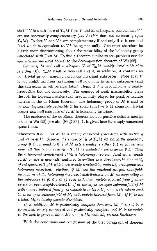
Holonomy Groups and General Relativity 235
that if V is a subspace of TmM then V and its orthogonal complement V' are not necessarily complementary (i.e. V U V' does not necessarily span T m M ) . In fact V and V L are complementary if and only if V is non-null (and which is equivalent to V' being non-null). One must therefore be a little more discriminating about the reducibility of the holonomy group associated with I? on M . To find a theorem similar to the previous one for space-times one must appeal to the decomposition theorem of Wu [98].
Let m E M and call a subspace V of T m M weakly irreducible if it is either {0}, T,M itself or non-null and if, in addition, it contains no non-trivial proper non-null holonomy invariant subspaces. Note that V is not prohibited from containing null holonomy invariant subspaces (and this can occur as will be clear later). Hence if V is irreducible it is weakly irreducible but not conversely. The concept of weak irreducibility plays the role for Lorentz metrics that irreducibility played for positive definite metrics in the de Rham theorem. The holonomy group of M is said to be non-degenerately reducible if for some (any) m E M some non-trivial proper non-null subspace of Tm M is holonomy invariant.
The analogue of the de Rham theorem for non-positive definite metrics is due to Wu [98] (see also [99],[100]). It is given here for simply connected space-times.
Theorem 8.8 Let M be a simply connected space-time with metric g and let m E M . Suppose the subspace VO of T m M on which the holonomy group @ (now equal to @') of M acts trivially is either (0) or proper and non-null (the trivial case VO = T m M is excluded - see theorem 8.4). Then the orthogonal complement of VO is holonomy invariant (and either equals T m M or else is non-null) and may be written as a direct sum Vl @ . . . @ v k
of subspaces of T m M which are weakly irreducible, mutually orthogonal and holonomy invariant. Further, i f M i are the maximal integral manifolds through m of the holonomy invariant distributions on M corresponding to the subspaces I4 (0 6 i 6 k ) each with their metric induced from g there exists an open neighbourhood U of m which, as an open submanijold of M with metric induced f r o m g , is isometric to UO x U1 x . x u k where each Ui is an open submanifold of M i with metric induced f rom M i . I f Vo is not trivial, MO is locally pseudo-Euclidean.
If, in addition, M is geodesically complete then each Mi (0 6 i < k ) is connected, simply connected and geodesically complete and M is isometric to the metric product MO x M I x ' ., x Mk with M O pseudo-Euclidean.
With the conditions and conclusions of the first paragraph of theorem
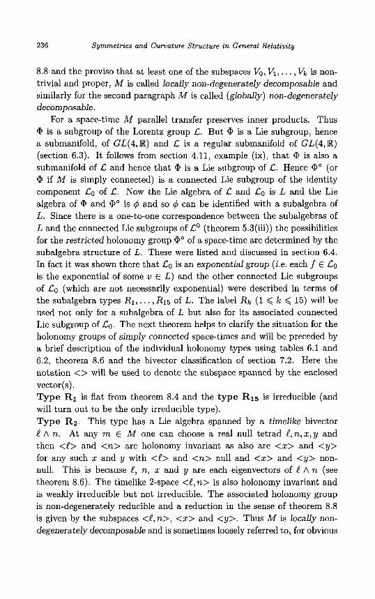
236 Symmetries and Curvature Stwcture in General Relativity
8.8 and the proviso that at least one of the subspaces VO, V1, . . . , v k is non- trivial and proper, M is called locally non-degenerately decomposable and similarly for the second paragraph M is called (globally) non-degenerately decomposable.
For a space-time M parallel transfer preserves inner products. Thus @ is a subgroup of the Lorentz group L. But @ is a Lie subgroup, hence a submanifold, of GL(4,R) and L is a regular submanifold of GL(4,R) (section 6.3). It follows from section 4.11, example (ix), that @ is also a submanifold of L and hence that @ is a Lie subgroup of C. Hence a' (or @ if M is simply connected) is a connected Lie subgroup of the identity component LO of C. Now the Lie algebra of C and LO is L and the Lie algebra of @ and a' is q5 and so q5 can be identified with a subalgebra of L. Since there is a one-to-one correspondence between the subalgebras of L and the connected Lie subgroups of Lo (theorem 5.3(iii)) the possibilities for the restricted holonomy group @' of a space-time are determined by the subalgebra structure of L. These were listed and discussed in section 6.4. In fact it was shown there that LO is an exponential group (i.e. each f E CO is the exponential of some v E L) and the other connected Lie subgroups of CO (which are not necessarily exponential) were described in terms of the subalgebra types R1 , .. . , R15 of L. The label R k (1 < Ic < 15) will be used not only for a subalgebra of L but also for its associated connected Lie subgroup of LO. The next theorem helps to clarify the situation for the holonomy groups of simply connected space-times and will be preceded by a brief description of the individual holonomy types using tables 6.1 and 6.2, theorem 8.6 and the bivector classification of section 7.2. Here the notation <> will be used to denote the subspace spanned by the enclosed vector(s). Type R1 is flat from theorem 8.4 and the type R15 is irreducible (and will turn out to be the only irreducible type). Type RZ. This type has a Lie algebra spanned by a timelike bivector C A n. At any m E M one can choose a real null tetrad !,n,x,y and then <e> and <n> are holonomy invariant as also are <x> and <y> for any such x and y with <e> and <n> null and <x> and <y> non- null. This is because e, n, x and y are each eigenvectors of e A n (see theorem 8.6). The timelike 2-space <el n> is also holonomy invariant and is weakly irreducible but not irreducible. The associated holonomy group is non-degenerately reducible and a reduction in the sense of theorem 8.8 is given by the subspaces 4, n>, <x> and <y>. Thus M is locally non- degenerately decomposable and is sometimes loosely referred to, for obvious
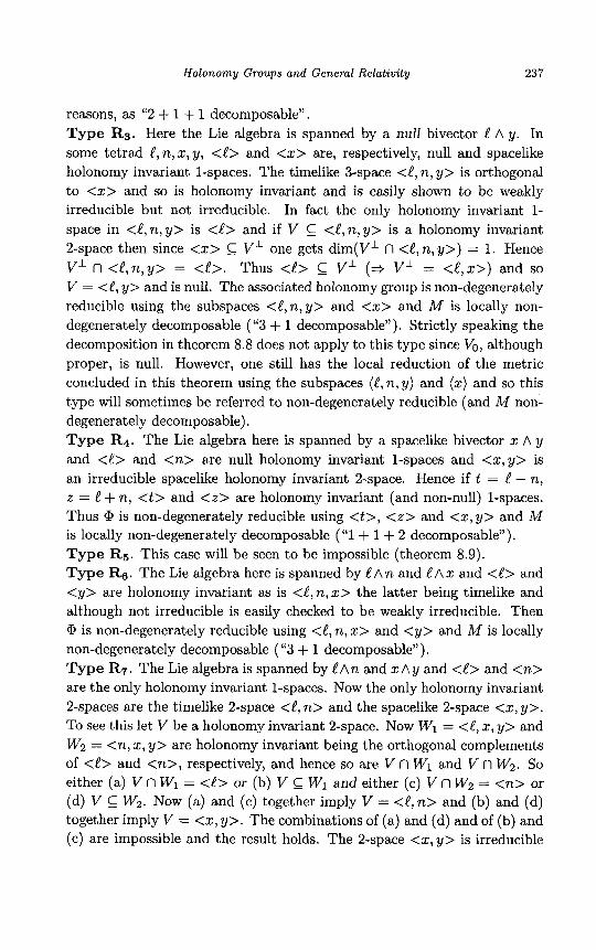
Holonomy Groups and General Relativity 237
reasons, as “2 + 1 + 1 decomposable”. Type Rs. Here the Lie algebra is spanned by a null bivector C A y. In some tetrad C, n, x , y, <C> and <x> are, respectively, null and spacelike holonomy invariant 1-spaces. The timelike 3-space <I, n, y> is orthogonal to <x> and so is holonomy invariant and is easily shown to be weakly irreducible but not irreducible. In fact the only holonomy invariant 1- space in <C, n, y> is <C> and if V G <C, n, y> is a holonomy invariant 2-space then since <x> V’ one gets dim(V’ n <C, n, y>) = 1. Hence V’ n <C,n, y> = <I>. Thus <C> C V’ (3 V’ = <C,x>) and SO
V = <e, y> and is null. The associated holonomy group is non-degenerately reducible using the subspaces <C, n, y> and <x> and M is locally non- degenerately decomposable ( “3 + 1 decomposable”). Strictly speaking the decomposition in theorem 8.8 does not apply to this type since V,, although proper, is null. However, one still has the local reduction of the metric concluded in this theorem using the subspaces ( C , n, y) and (x) and so this type will sometimes be referred to non-degenerately reducible (and M non- degenerately decomposable). Type R d . The Lie algebra here is spanned by a spacelike bivector x A y and <C> and <n> are null holonomy invariant 1-spaces and < x , y > is an irreducible spacelike holonomy invariant 2-space. Hence if t = C - n, z = C + n, <t> and <z> are holonomy invariant (and non-null) 1-spaces. Thus @ is non-degenerately reducible using <t>, <z> and <x, y > and M is locally non-degenerately decomposable (“1 + 1 + 2 decomposable”). Type R g . This case will be seen to be impossible (theorem 8.9). Type Re. The Lie algebra here is spanned by e A n and e A x and <e> and <y> are holonomy invariant as is <C,n,x> the latter being timelike and although not irreducible is easily checked to be weakly irreducible. Then @ is non-degenerately reducible using <C, n, x> and <y> and M is locally non-degenerately decomposable ( “3 + 1 decomposable”). Type R7. The Lie algebra is spanned by CAn and X A y and <C> and <n> are the only holonomy invariant 1-spaces. Now the only holonomy invariant 2-spaces are the timelike 2-space <I, n> and the spacelike 2-space <x, y>. To see this let V be a holonomy invariant 2-space. Now Wl = <el x , y> and W2 = <n, x , y> are holonomy invariant being the orthogonal complements of <C> and <n>, respectively, and hence so are V n W1 and V n W2. So either (a) V n WI = <C> or (b) V C W1 and either (c) V n W2 = <n> or (d) V C W,. Now (a) and (c) together imply V = <P,n> and (b) and (d) together imply V = <x, y>. The combinations of (a) and (d) and of (b) and (c) are impossible and the result holds. The 2-space <x, y> is irreducible
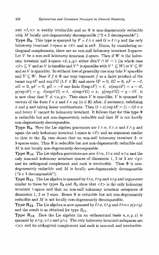
238 Symmetries and Curvature Structure in General Relativity
and <C,n> is weakly irreducible and so Q is non-degenerately reducible with M locally non-degenerately decomposable (“2 + 2 decomposable”). Type RE,. This type is spanned by F = C A x and G = C A y and the only holonomy invariant 1-space is <C> and is null. Hence, by considering or- thogonal complements, there are no non-null holonomy invariant 3-spaces. Let V be a non-null holonomy invariant 2-space. Then if W is the holon- omy invariant null 3-space <e, x, y> either dim V n W = 1 (in which case <e> G V and so V is timelike and VL is spacelike with V’- C W ) or V g W and so V is spacelike. So without loss of generality one may take V spacelike and V W . Now if f E Q one may represent f as a finite product of the terms exp t F and exp t’G ( t , t’ E W) and since CF = 0, CG = 0, XF = -C, XG = 0, y F = 0, yG = -C one finds C(exptF) = e, x(exptF) = x - t t , y(exptF) = y, C(expt’G) = C, x(expt’G) = X, y(expt’G) = y - t’C. It is now clear that V # <x, y>. Thus since V is spacelike, V is spanned by vectors of the form C + x and C + a y (0 E W) after, if necessary, redefining x and y and taking linear combinations. Then (C + x) exp t F = (1 - t)! + x and hence V cannot be holonomy invariant. It follows that for this type Q is reducible but not non-degenerately reducible and that M is not locally non-degenerately decomposable. Type R9. Here the Lie algebra generators are e A n, e A x and e A y and again the only holonomy invariant 1-space is <C> and an argument similar to that in the Rg case shows that no non-null holonomy invariant 2- or 3-spaces exist. Thus is reducible but not non-degenerately reducible and M is not locally non-degenerately decomposable. Type Rlo. The Lie algebra generators are now [ A n , CAx and nAx and the only non-null holonomy invariant spaces of dimension 1, 2 or 3 are <y> and its orthogonal complement and each is irreducible. Thus Q is non- degenerately reducible and M is locally non-degenerately decomposable ( “3 + 1 decomposable”). Type R11. The Lie algebra is spanned by [Ax, CAY and xAy and arguments similar to those for types Rg and Rg show that <C> is the only holonomy invariant 1-space and that no non-null holonomy invariant subspaces of dimension 1, 2 or 3 exist. Hence Q is reducible but not non-degenerately reducible and M is not locally non-degenerately decomposable. Type Rlz. The Lie algebra is now spanned by CAx, CAy and CAn+p(xAy) and the result is as obtained for type R11.
Type R13. Here the Lie algebra (in an orthonormal basis u, x, y, z ) is spanned by xAy, x A z and yAz. The only holonomy invariant subspaces are <u> and its orthogonal complement and each is non-null and irreducible.
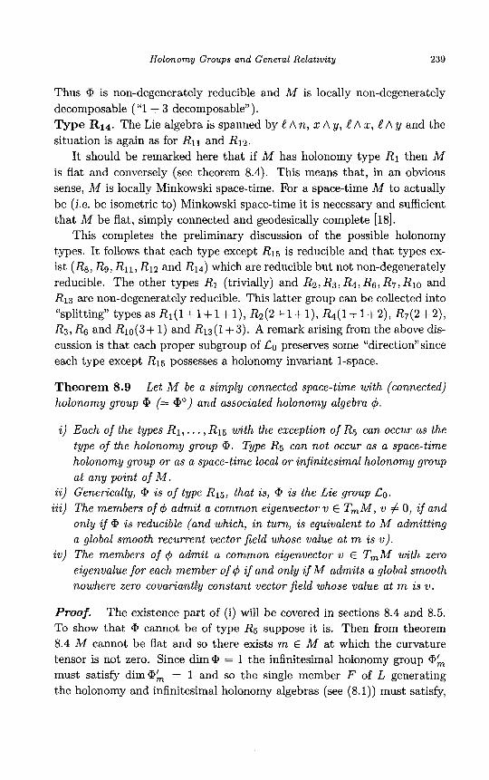
Holonomy Groups and General Relativity 239
Thus CI, is non-degenerately reducible and M is locally non-degenerately decomposable (“1 + 3 decomposable”). Type R14. The Lie algebra is spanned by C A n, x A y, !A x, !A y and the situation is again as for R11 and R12.
It should be remarked here that if M has holonomy type R1 then M is flat and conversely (see theorem 8.4). This means that, in an obvious sense, M is locally Minkowski space-time. For a space-time M to actually be (ie. be isometric to) Minkowski space-time it is necessary and sufficient that M be flat, simply connected and geodesically complete [18].
This completes the preliminary discussion of the possible holonomy types. It follows that each type except R15 is reducible and that types ex- ist (Rs, Rg, R11, Rl2 and R14) which are reducible but not non-degenerately reducible. The other types R1 (trivially) and R2, R3, R4, Re, R7, Rlo and R13 are non-degenerately reducible. This latter group can be collected into “splitting” types as R1(1+ 1 + 1 + l), R2(2 + 1 + l), R4( 1 + 1 + 2 ) , R7(2 + 2 ) , R3, Rg and Rlo (3 + 1 ) and R13 (1 + 3). A remark arising from the above dis- cussion is that each proper subgroup of 130 preserves some “direction”since each type except R15 possesses a holonomy invariant 1-space.
Theorem 8.9 holonomy group @ (= a’) and associated holonomy algebra 4.
Let M be a simply connected space-time with (connected)
i) Each of the types R1,. . . , R15 with the exception o f R5 can occur as the type of the holonomy group @. Type R5 can not occur as a space-time holonomy group or as a space-time local or infinitesimal holonomy group at any point of M .
ii) Generically, Q, is of type R15, that is, @ is the Lie group 130. iii) The members of q? admit a common eigenvector v E T,M, v # 0 , i f and
only i f Q, is reducible (and which, in turn, is equivalent to M admitting a global smooth recurrent vector field whose value at m is u).
i v ) The members of 4 admit a common eigenvector u E T,M with zero eigenvalue fo r each member of q? i f and only i f M admits a global smooth nowhere zero covariantly constant vector field whose value at m is v.
Proof. The existence part of (i) will be covered in sections 8.4 and 8.5. To show that Q, cannot be of type Rs suppose it is. Then from theorem 8.4 M cannot be flat and so there exists m E M at which the curvature tensor is not zero. Since dim@ = 1 the infinitesimal holonomy group CI,& must satisfy d i m a h = 1 and so the single member F of L generating the holonomy and infinitesimal holonomy algebras (see (8.1)) must satisfy,

240 Symmetries and Curvature Structure in General Relativity
in component form, Rabcd = a F a b F c d at m for 0 # a E R. But then R a [ b c d ] = 0 * F [ a b F c ] d = 0 * F is a simple bivector (theorem 7.1) and this contradicts the fact that the generator for the R5 subalgebra is not simple [[101],[102] - see also [45],[103]]. This proof contains within it the impossibility of a type Rs local or infinitesimal holonomy group at any m E M .
In (ii) one uses the generic condition described in theorem 7.18 to see that, generically on the set of smooth Lorentz metrics on M , there exists m E M at which the curvature tensor has rank equal to 6 and hence that dim@; = 6. Hence, since dim,& = 6 one sees that @; and @’ (and @) coincide with LO and the holonomy type is R 1 5 generically.
In (iii) if such a vector v exists then it follows from theorem 8.6 that Q, is reducible. Conversely if @ is reducible then the remarks immediately before this theorem show that at m E M there exists a holonomy invariant 1-space spanned, say, by v E T,M and hence, by theorem 8.6, v is an eigenvector of each member of the holonomy algebra 4. Theorem 8.6 then shows that for each m E M there is an open neighbourhood U of m and a smooth nowhere zero recurrent vector field X on U which belongs to the holonomy invariant distribution generated by v and thus this “direction” is well defined globally on M . Now M , being paracompact, admits a global smooth positive definite metric y (theorem 4.14). The vector field X defined on U above is defined only to within a smooth nowhere zero scaling factor and can (and will) be replaced on U by the vector field X’ = [ y ( X , X ) ] - 1 / 2 X so that ?(XI , X I ) = 1. (It is easily checked that if X is recurrent on U then so is f X for f : U -+
Iw \ ( 0 ) and so X’ is recurrent on U . ) Now M can be covered by connected coordinate neighbourhoods such as U above and the vector fields X‘ arising on each such U agree up to a sign wherever such neighbourhoods intersect. The construction of a global recurrent vector field on M can now be briefly described. First consider the set M which is the set theoretic union of all such subsets U each taken twice, once with each sign for X’ (so that each point of M is a point m E M and a choice of either X‘(m) or -X’ (m) ) , Then is a 4-dimensional manifold with the above modified subsets as an atlas. [To see these coordinate neighbourhoods of M satisfy the intersection property for manifolds let p : h;r -+ A4 be the obvious smooth projection map defined by preserving the point of fi in M but “forgetting” the sign for X‘. Then if 01 and 0 2 are such coordinate neighbourhoods in M with associated vector fields X I and X2 and if f i E O1nO2 then X l ( m ) = X2(m) where m = p ( f i ) . Then if U I = p ( 0 1 ) , U2 = p ( 0 2 ) , the definition of X’ shows that there exists an open neighbourhood U, of m in M such that
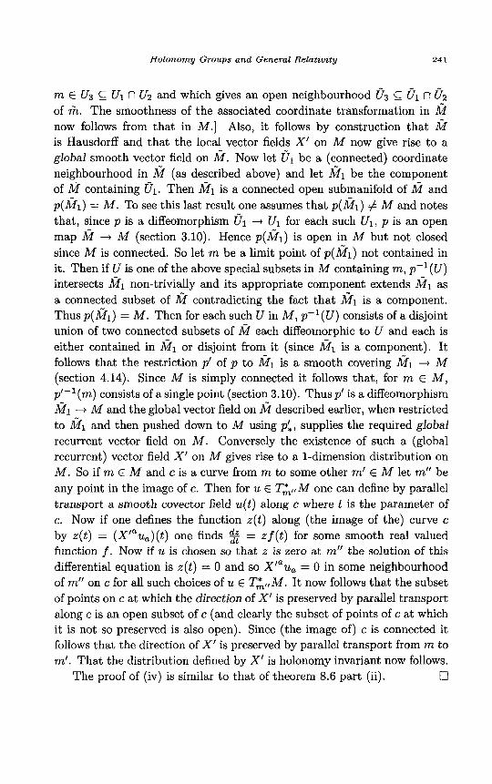
Holonomy Groups and General Relativity 24 1
m E Us U1 f l U2 and which gives an open neighbourhood 0 3 C 01 1-102
of 6. The smoothness of the associated coordinate transformation in M now follows from that in M.] Also, it follows by construction that &f is Hausdorff and that the local vector fields X' on M now give rise to a global smooth vector field on &f. Now let 01 be a (connected) coordinate neighbourhood in fi (as described above) and let h;r, be the component of &l containing 01. Then M 1 is a connected open submanifold of M and p ( G 1 ) = M . To see this last result one assumes that p ( f i 1 ) # M and notes that, since p is a diffeomorphism 01 -+ U1 for each such U1, p is an open map -i M (section 3.10). Hence p(h;r,) is open in M but not closed since M is connected. So let m be a limit point of p ( f i 1 ) not contained in it. Then if U is one of the above special subsets in M containing m, p - l ( U )
intersects non-trivially and its appropriate component extends f i 1 as a connected subset of M contradicting the fact that M I is a component. Thus p(M1) = M . Then for each such U in M , p- ' (U) consists of a disjoint union of two connected subsets of A?l each diffeomorphic to U and each is either contained in or disjoint from it (since 2 1 is a component). It follows that the restriction p' of p to M I is a smooth covering -i M (section 4.14). Since M is simply connected it follows that, for m E M , p'-' (m) consists of a single point (section 3.10). Thus p' is a diffeomorphism
.--t M and the global vector field on M described earlier, when restricted to and then pushed down to M using p i , supplies the required global recurrent vector field on M . Conversely the existence of such a (global recurrent) vector field X' on M gives rise to a 1-dimension distribution on M . So if m E M and c is a curve from m to some other m' E M let m'' be any point in the image of c. Then for u E T&M one can define by parallel transport a smooth covector field u(t) along c where t is the parameter of c. Now if one defines the function z ( t ) along (the image of the) curve c by z ( t ) = (X'"u,)(t) one finds 8 = zf(t) for some smooth real valued function f . Now if u is chosen so that z is zero at m'' the solution of this differential equation is z ( t ) = 0 and so X ' a ~ a = 0 in some neighbourhood of m" on c for all such choices of u E T;,, M . It now follows that the subset of points on c at which the direction of X' is preserved by parallel transport along c is an open subset of c (and clearly the subset of points of c at which it is not so preserved is also open). Since (the image of) c is connected it follows that the direction of X' is preserved by parallel transport from m to m'. That the distribution defined by X' is holonomy invariant now follows.
cl The proof of (iv) is similar to that of theorem 8.6 part (ii).
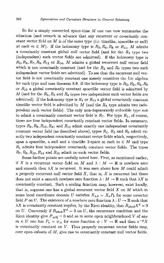
242 Symmetries and Curvature Structure in General Relativity
So for a simply connected space-time M one can now summarise the situation (and remark in advance that any recurrent or covariantly con- stant vector field on M is of the same type (i.e. timelike, spacelike or null) a t each m E M ) . If the holonomy type is R3, R4, Rg or R11, M admits a covariantly constant global null vector field (and for the R4 type two (independent) such vector fields are admitted). If the holonomy type is R2, R6, R7, Rg, R 1 2 or R14, M admits a global recurrent null vector field which is not covariantly constant (and for the Rz and R7 types two such independent vector fields are admitted). To see that the recurrent null vec- tor field is not covariantly constant one merely considers the Lie algebra for each type and uses theorem 8.9. If the holonomy type is R2, R3, Rq, & or Rlo a global covariantly constant spacelike vector field is admitted by M (and for the R2, R3 and R4 types two independent such vector fields are admitted). If the holonomy type is R4 or R13 a global covariantly constant timelike vector field is admitted by M (and the R4 type admits two inde- pendent such vector fields). The only non-degenerately reducible type not to admit a covariantly constant vector field is R7. For type R1, of course, there are four independent covariantly constant vector fields. In summary, types Re, Rg, Rlo, R11 and R13 admit exactly one independent covariantly constant vector field (as described above), types R2, R3 and R4 admit ex- actly two independent covariantly constant vector fields which, respectively, span a spacelike, a null and a timelike 2-space at each m E M and type R1 admits four independent covariantly constant vector fields. The types R7, Rs, R12, R14 and R15 admit no such vector fields.
Some further points are usefully noted here. First, as mentioned earlier, if X is a recurrent vector field on M and X : M + R is nowhere zero and smooth then AX is recurrent. It was seen above how M could admit a properly recurrent null vector field X , that is, X is recurrent but there does not exist a smooth nowhere zero function X : M -+ R such that AX is covariantly constant. Such a scaling function may, however, exist locally, that is, suppose one has a global recurrent vector field X on M which in some local coordinate domain U satisfies X a ; b = XaPb for some covector field P on U . The existence of a nowhere zero function X : U 4 R such that AX is covariantly constant implies, by the Ricci identity, that RabcdXd = 0 on U . Conversely if RabcdXd = 0 on U , the recurrence condition and the Ricci identity give P[.;b] = 0 and so in some open neighbourhood V of any m E U one has Pa = 1CI9 , for some function $ : V + R and then e-*X is covariantly constant on V . Thus properly recurrent vector fields may, over open subsets of M , give rise to covariantly constant null vector fields.

Holonomy Groups and General Relativity 243
This argument is quite general. If M is simply connected, X recurrent and RabcdXd = 0 on M then the consequent condition q a ; b l = 0 on M reveals a global function $J : M --t JR (section 4.16) such that Pa = and so e-$X is a global covariantly constant vector field on M . Hence if M is simply connected, a recurrent vector field X on A4 can be globally scaled so as to be covariantly constant if and only if RabcdXd = 0 on M . The idea of proper recurrence is restricted to null vector fields in the sense that if X is a global recurrent non-null vector field on M then the global vector field X‘ = Ig(X,X)I-’/2X is covariantly constant on M . To see this note that X‘”X’, is constant and non-zero and that X’ is also recurrent (and so in any local coordinate system X’a;b = X’aPb). A contraction with X’” gives Pb = 0 in this (and any other) coordinate domain and the result follows. Bearing in mind theorem 8.9 this is essentially the result that a non-null eigenvector of a bivector necessarily has a zero eigenvalue. The types Rz, &, R7, Rg, Rl2 and R14 admit a properly recurrent null vector field (and R2 and R7 admit two independent such fields).
For those simply connected space-times which are locally non- degenerately decomposable (ie. @ (= @’) non-degenerately reducible) one has a convenient form for the metric and which arises from the fact that from theorem 8.8 each m E M has a neighbourhood which is locally a met- ric product of manifolds (and which explains the “splitting types” given earlier).
For holonomy type R13 (splitting type 1 + 3) and for m E M one may decompose “,A4 as VO @ V1 with dim VO = 1 and dim V1 = 3 (as in theorem 8.8). Then one may choose a product coordinate neighbourhood U of the type described in theorem 8.8 (with U = I x V where I is an open interval of E% and V an open connected subset of R3) about m and coordinates t , xa (a = 1 ,2 ,3 ) such that, in U, the metric g takes the form
ds2 = -dt2 + gapdxadzP (p = 1 ,2 ,3 ) (8.3)
where the gap are independent oft . The vector field & on U agrees (on U) with the global covariantly constant timelike vector field admitted by M . The components gap give rise to a positive definite metric on the submani- folds t = constant of U and two such submanifolds, say t = t o and t = tl are isometric under the diffeomorphism ( t o , xa) -+ (t l , xa) on U (“following the integral curves s 4 (s, O , O , 0) of &”). For the metric (8.3) the only non- vanishing Christoffel symbols are those of the form r& (a, p, y = 1 ,2 ,3 ) and these are easily checked to be the Christoffel symbols of the metric gap. Similarly, the only non-vanishing curvature tensor components are of
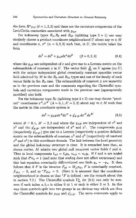
244 Symmetries and Curvature Structure in General Relativity
the form R"p76 (6 = 1,2 ,3) and these are the curvature components of the Levi-Civita connection associated with gap .
For holonomy types R3, Rs and Rlo (splitting type 3 + 1) one may similarly choose a product coordinate neighbourhood U about any m E M and coordinates x, x" (0 = 0 , 2 , 3) such that, in U, the metric takes the form
where the gao are independent of x and give rise to a Lorentz metric on the submanifolds of constant x in U . The vector field & on U agrees (on U ) with the unique independent global covariantly constant spacelike vector field admitted by M in the R6 and R l o types and one of the family of such vector fields in the R3 case. The submanifolds of constant x are isometric as in the previous case and the comments regarding the Christoffel sym- bols and curvature components made in the previous case (appropriately modified) also hold.
For the holonomy type R7 (splitting type 2 + 2) one may choose "prod- uct" coordinates xA , xA' ( A = 0,1, A' = 2,s) about any m € M such that the metric in this coordinate system is
where B = 0,1, B' = 2 , 3 and where the g A B are independent of x2 and x3 and the gk tB t are independent of xo and xl. The components g A B (respectively g a l B l ) give rise to a Lorentz (respectively a positive definite) metric on the submanifolds of constant x2 and z3 (respectively of constant xo and x l ) in this coordinate domain. The link between the local geometry and the global holonomy structure is clear. It is remarked here that, as shown earlier, M admits two global null recurrent vector fields l and n. Thus in local components &;b = &Pb, n a ; b = naqb, If C and n are scaled such that lana = 1 (and note that scaling does not affect recurrence) and this last equation covariantly differentiated one finds qa = -pa. It then follows that if F is the bivector Fab = 2l[,nb], F is covariantly constant, Fab;c = 0, and so *Fabic = 0. (Here it is assumed that the coordinate neighbourhood is chosen so that * F is defined - see the remark about this in section 7.2.) The Christoffel symbols I?& for (8.5) can only be non- zero if each index a, b, c is either 0 or 1 or each is either 2 or 3. In this way these symbols split into two groups in an obvious way which are then the Christoffel symbols for g A B and g>rB,. The same comments apply to
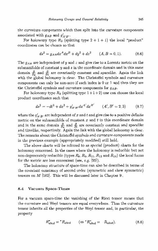
Holonomy Groups and General Relativity 245
the curvature components which then split into the curvature components associated with gAB and g k f B , .
For holonomy type R 2 (splitting type 2 + 1 + 1) the local "product" coordinates can be chosen so that
The gAB are independent of y and z and give rise to a Lorentz metric on the submanifolds of constant y and z in the coordinate domain and in this same domain & and 2 are covariantly constant and spacelike. Again the link with the global holonomy is clear. The Christoffel symbols and curvature components can only be non-zero if each index is 0 or 1 and then they are the Christoffel symbols and curvature components for gAB.
For holonomy type R 4 (splitting type 1 + 1 + 2) one can choose the local product coordinates such that
ds2 = -dt2 + d x 2 + gL,,,dxA'dxB' (A', B' = 2 ,3 ) (8.7)
where the ga ,B , are independent of x and t and give rise to a positive definite metric on the submanifolds of constant x and t in this coordinate domain and in the same domain & and 3 are covariantly constant and spacelike and timelike, respectively. Again the link with the global holonomy is clear. The remarks about the Christoffel symbols and curvature components made in the previous example (appropriately modified) still hold.
The above charts will be referred to as special (product) charts for the holonomy concerned. In the cases where the holonomy is reducible but not non-degenerately reducible (types Rs, Rg, Rll, R 1 2 and R 1 4 ) the local forms for the metric are less convenient (see, e.g. [55]).
The holonomy structure of space-time can also be described in terms of the covariant constancy of second order (symmetric and skew symmetric) tensors on A4 [102]. This will be discussed later in Chapter 9.,
8.4 Vacuum Space-Times
For a vacuum space-time the vanishing of the Rcci tensor means that the curvature and Weyl tensors are equal everywhere. Thus the curvature tensor inherits all the properties of the Weyl tensor and, in particular, the property
R:bcd = * R a b c d (6 *R:bcd = - R a b c d ) . (8.8)

246 Symmetries and Curvature Structure in General Relativity
This enables a simple and useful property of the infinitesimal holonomy algebra and group to be established [104] (cf. [45]).
Lemma 8.1 Let M be a vacuum space-time. Then at any m E M the infinitesimal holonomy group is of type R1, Rs, R14 or Rls and all these types are possible (as will be clear f rom section 8.5).
Proof. matrices in (8.1) one notes that because of (8.8)
Thinking of the infinitesimal holonomy algebra in terms of the
and so on. Thus a certain (skew-symmetric) matrix is a member of the infinitesimal holonomy algebra 4; if and only if its dual is. From this it follows (not completely trivially) that dim& is even (or 0). To see this suppose F E 4;. Then * F E 4; and so, if there are no further independent members of $Al dim$; = 2. If there is a third independent member G E #& then 'G E 4',. Now F, *F,G and *G are independent members of 4; because if
crF + 0 * F + yG + 6 *G = 0 (a , 0, y, 6 E IR and not all zero)
then the independence of F, * F and G shows that 6 # 0 and a similar argument applied to the dual of the above relation shows that y # 0. Then the above relation and its dual can be used to eliminate *G. This shows that (y2 + S2)G is a linear combination of F and * F and this contradiction shows that F , * F , G and *G are independent. If no other independent members of 4; exist then dim 4; = 4. If they do then dim 4; = 6 either by repeating the previous argument or by reference to the classification of the subalgebras of the Lorentz algebra since no such subalgebra has dimension 5. The facts that dim I$& is even and that F E 4; * * F E 4; now shows that the only possibilities for the type of 4; are R1, R7, RB, R14 and R15 (table 6.1).
If for some m E M the type of 4; is R7 then a consideration of table 6.1 and equation (8.1) shows that if F represents the bivector C A n in the table then there exist 0, 0, y, E W and tensors P, &, S at m such that the
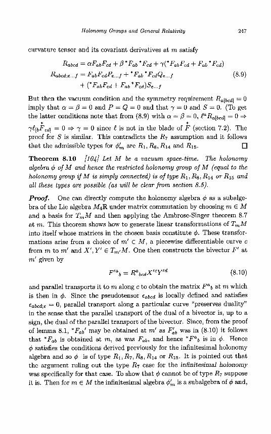
H o l o n o m y Groups and General Relat iv i ty 247
curvature tensor and its covariant derivatives at m satisfy
Rabcd = f f F a b F c d + P * F a b *Fed + y ( * F a b F c d -I- F a b *Fed) Rabcd;e ... f = F a b F c d P e ...f + * F a b * F c dQe ...f (8.9)
+ ( * F a b F c d + F a 6 * F c d ) S e ... f
But then the vacuum condition and the symmetry requirement Ra[bcd] = 0 imply that a = P = 0 and P = Q = 0 and that y = 0 and S = 0. (To get the latter conditions note that from (8.9) with a = P = 0 , taRapcd] = 0 3
$ [ b F c d ] = 0 =+ y = 0 since c is not in the blade of F (section 7.2). The proof for S is similar. This contradicts the R7 assumption and it follows
Theorem 8.10 The holonomy algebra 4 of M and hence the restricted holonomy group of M (equal t o the holonomy group if M is simply connected) i s of type R 1 , R 8 , R 1 4 or R l 5 and all these types are possible (as will be clear f rom section 8.5).
Proof. One can directly compute the holonomy algebra 4 as a subalge- bra of the Lie algebra M4R under matrix commutation by choosing m E M and a basis for TmM and then applying the Ambrose-Singer theorem 8.7 at m. This theorem shows how to generate linear transformations of T, M into itself whose matrices in the chosen basis constitute 4. These transfor- mations arise from a choice of m' E M , a piecewise differentiable curve c from m to m' and X ' , Y' E Tmt M . One then constructs the bivector F' at m' given by
* *
that the admissible types for & are R 1 , Rs, R 1 4 and R 1 5 .
[lo41 Let M be a vacuum space-time.
F l a b = R a b c d X ' C Y ' d (8.10)
and parallel transports it to m along c to obtain the matrix F a b at m which is then in 4. Since the pseudotensor Eabcd is locally defined and satisfies €abcd;e = 0, parallel transport along a particular curve "preserves duality" in the sense that the parallel transport of the dual of a bivector is, up to a sign, the dual of the parallel transport of the bivector. Since, from the proof of lemma 8.1, *Fab' may be obtained at m' as FLb was in (8.10) it follows that * F a b is obtained at m, as was F a b , and hence * F a b is in 4. Hence 4 satisfies the conditions derived previously for the infinitesimal holonomy algebra and so 4 is of type R1, R 7 , Rs, R 1 4 or R 1 5 . It is pointed out that the argument ruling out the type R 7 case for the infinitesimal holonomy was specifically for that case. To show that 4 cannot be of type R7 suppose it is. Then for m E M the infinitesimal algebra &, is a subalgebra of and,
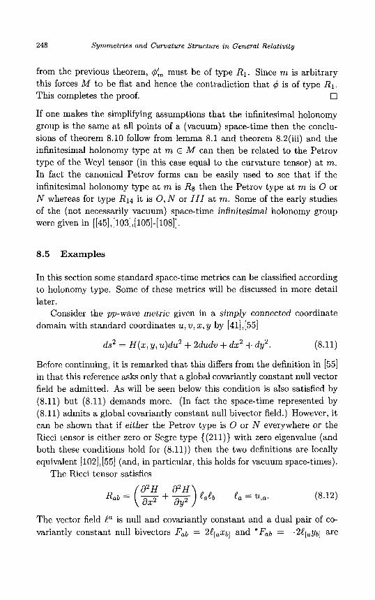
248 Symmetries and Curvature Structure in General Relativity
from the previous theorem, q5& must be of type R1. Since m is arbitrary this forces M to be flat and hence the contradiction that q5 is of type R1. This completes the proof. 0
If one makes the simplifying assumptions that the infinitesimal holonomy group is the same at all points of a (vacuum) space-time then the conclu- sions of theorem 8.10 follow from lemma 8.1 and theorem 8.2(iii) and the infinitesimal holonomy type at m E M can then be related to the Petrov type of the Weyl tensor (in this case equal to the curvature tensor) at m. In fact the canonical Petrov forms can be easily used to see that if the infinitesimal holonomy type at m is R8 then the Petrov type at m is 0 or N whereas for type R14 it is 0, N or 111 at m. Some of the early studies of the (not necessarily vacuum) space-time infinitesimal holonomy group were given in [[45],[103],[105]-[108]].
8.5 Examples
In this section some standard space-time metrics can be classified according to holonomy type. Some of these metrics will be discussed in more detail later.
Consider the pp-wave metric given in a simply connected coordinate domain with standard coordinates u, v, 2 , y by [41],[55]
ds2 = H ( x , y, u)du2 + 2dudv + dz2 + dy2. (8.11)
Before continuing, it is remarked that this differs from the definition in [55] in that this reference asks only that a global covariantly constant null vector field be admitted. As will be seen below this condition is also satisfied by (8.11) but (8.11) demands more. (In fact the space-time represented by (8.11) admits a global covariantly constant null bivector field.) However, it can be shown that if either the Petrov type is 0 or N everywhere or the Ricci tensor is either zero or Segre type ((211)) with zero eigenvalue (and both these conditions hold for (8.11)) then the two definitions are locally equivalent [102], [55] (and, in particular, this holds for vacuum space-times).
The Ricci tensor satisfies
Rab = ($ + e) eaeb e, = u,a. dY2
(8.12)
The vector field la is null and covariantly constant and a dual pair of co- variantly constant null bivectors Fab = 2!?[aXb] and * F a b = -2!?[,yb] are
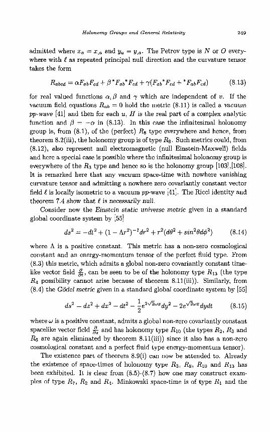
Holonomy Groups and Geneml Relativity 249
admitted where x , = x , ~ and ya = y,,. The Petrov type is N or 0 every- where with C as repeated principal null direction and the curvature tensor takes the form
Rabcd = QFabFcd + P*Fab*Fcd + Y(Fab*Fcd f *FabFcd) (8.13)
for real valued functions a,/3 and y which are independent of v. If the vacuum field equations Rat, = 0 hold the metric (8.11) is called a vacuum pp-wave [41] and then for each u, H is the real part of a complex analytic function and /3 = -a in (8.13). In this case the infinitesimal holonomy group is, from (8.1), of the (perfect) R8 type everywhere and hence, from theorem 8.2(iii), the holonomy group is of type R8. Such metrics could, from (8.12), also represent null electromagnetic (null Einstein-Maxwell) fields and here a special case is possible where the infinitesimal holonomy group is everywhere of the R3 type and hence so is the holonomy group [103],[108]. It is remarked here that any vacuum space-time with nowhere vanishing curvature tensor and admitting a nowhere zero covariantly constant vector field C is locally isometric to a vacuum ppwave [41]. The Rcci identity and theorem 7.4 show that C is necessarily null.
Consider now the Einstein static universe metric given in a standard global coordinate system by [55]
ds2 = -dt2 + (1 - Ar2)- 'dr2 + r2(d02 + sin28d$2) (8.14)
where A is a positive constant. This metric has a non-zero cosmological constant and an energy-momentum tensor of the perfect fluid type. From (8.3) this metric, which admits a global non-zero covariantly constant time- like vector field &, can be seen to be of the holonomy type R13 (the type R4 possibility cannot arise because of theorem 8.1 1 (iii)). Similarly, from (8.4) the Godel metric given in a standard global coordinate system by [55]
1 ds2 = dz2 + dx2 - dt2 - - e z f iwXdy2 - 2e f iwxdyd t (8.15)
2
where w is a positive constant, admits a global non-zero covariantly constant spacelike vector field & and has holonomy type Rlo (the types R2, R3 and RS are again eliminated by theorem 8.ll(iii)) since it also has a non-zero cosmological constant and a perfect fluid type energy-momentum tensor).
The existence part of theorem 8.9(i) can now be attended to. Already the existence of space-times of holonomy type R3, Rg, Rlo and R13 has been exhibited. It is clear from (8.5)-(8.7) how one may construct exam- ples of type R7, Ra and Rq. Minkowski space-time is of type R1 and the
250 Symmetries and Curvature Structure in General Relativity
(vacuum) Schwarzschild metric is of type R15. This latter result is a conse- quence of the fact that for this metric the curvature tensor is easily checked to be everywhere of rank 6 (and so the infinitesimal holonomy type is R15
everywhere) and of theorem 8.2(iii). For the remaining types one notes that space-times which have these types as infinitesimal holonomy types every- where have been constructed in [105] and again theorem 8.2(iii) completes the argument. The vacuum type R14 examples in [105],[109],[110] complete the final sentences in lemma 8.1 and theorem 8.10. A study of the infinites- imal holonomy structure of Einstein-Maxwell fields was given in [lo31 and a detailed study of infinitesimal holonomy for arbitrary space-times (with some errors!) can be found in [108].
An investigation of the full holonomy group of a space-time was under- taken in [ l l l ] . In this work attention was directed to space-times with the more commonly studied energy-momentum tensors such as perfect fluids and null and non-null Einstein-Maxwell fields, and also to conformally flat space-times. For such space-times, convenient expressions for the curvature tensor can be obtained from (7.10) and (7.11). Then applications of the general techniques of this chapter yield the following theorem [ l l l ] .
Theorem 8.11 stein’s equations are assumed with zero cosmological constant. Then
Let M be a simply connected space-time on which Ein-
a) i f M is null Einstein-Maxwell with nowhere zero Maxwell tensor F and nowhere zero associated null direction e (section 7.7(a)), the holonomy group of M is of type R3, Ra, Rio, R14 or R15,
ii) i f M is non-null Einstein-Maxwell with nowhere zero associated energy- momentum tensor (section 7.7(a)), the holonomy group of M is of type
iii) i f M is a perfect fluid space-tame with fluid flow vector field u and with isotropic pressure p and energy density p in (7.7) and where M is not an Einstein space, the holonomy group of M is of type R ~ Q , R13 or R15,
iv) i f M is conformally flat but not flat, the holonomy group of M is of type R7, Ra, Rlo, R13, R14 orR.15,
v) if M is a proper Einstein space (i.e. the Ricci scalar R = constant # 0), the holonomy group of M is of type R7, R14 or R 1 5 .
R7, R14 or R15,
Proof. The general idea of the proof is to note that either the holonomy type is R15 or it is reducible (see the remarks just before theorem 8.9) and that in the latter case a global recurrent vector field is admitted from theorem 8.9. Proceeding with this latter case, with k the recurrent vector
Holonomy Groups and General Relativity 251
field, one uses the information on the energy-momentum tensor (or the Weyl tensor in part (iv)) and the Ambrose-Singer theorem 8.7 to achieve the results claimed. The perfect fluid case (iii) will be briefly established here and the proofs for the other cases can be found in [ l l l ] .
In (iii) one has from (7.7)
(8.16)
Now let k be a recurrent vector field on M . If k is, or can be scaled to be, covariantly constant (and this is always the case if k is not null) then the Ricci identity yields Rabcdkd = 0 and Rabkb = 0. If not, then k is null on M and ka;b = kapb for some global I-form p on M and the Kcci identity gives kaRabcd = kbFcd where Fab = 2p[a;b]. The algebraic Bianchi identity then gives k[,FbC] = 0 and so (section 7.2) F is a simple bivector whose blade contains k. It then follows that kaRab = Xkb for some function : M + R. Thus, whatever the recurrent vector field k is, it is a Ricci eigenvector, Rabkb = Aka. It then follows by contracting (8.16) with k b that
X l C , = 4 r ( p - P ) k a f 8 n ( p f p ) ( u b k b ) U a . (8.17)
Since k and u are nowhere zero on M it follows that if k is null, u a k a is nowhere zero on M and so p + p E 0 on M . Thus, from (8.16) M is an Einstein space and the clause in theorem S.ll(iii) is contradicted. If k is not null then, on M , one can assume that ka;b = 0 and X = 0. In particular, if k is timelike, uaka is never zero on M and (8.17) shows that either p - p = p+p = 0 on M (which means that M is a vacuum space-time and hence an Einstein space) or that u is proportional to k on M . Thus u is recurrent and, since uaua = -1, it is covariantly constant and one may assume u = k on M . Then Ua;b = 0 + R a b c d u d = 0 + R a b U b = 0 and, from (8.16), 3p + p = 0 on M . Thus
R a b = -16TP(gab + u a u b ) . (8.18)
The identity T a b ; b = 0 contracted with ua shows first that p,aua = 0 and then that p and p are each constant on M . The relation RabcdUd = 0 together with (8.18) then show that if (u, x, y, z ) is a pseudo-orthonormal tetrad at any m E M , then at m
Rabcd = -8nP(xabxcd + YabYcd f Z a b Z c d ) (8.19)
where X , Y and Z are, respectively, the bivectors x A y, x A z and y A z . It follows from (8.19) that the infinitesimal holonomy group, and hence the
252 Symmetries and Curvature Structure in General Relativity
holonomy group of M has dimension at least three and the existence of the covariantly constant timelike vector field k (or u) then shows the holonomy type is R13. If k is spacelike, the procedure is similar. One again finds X = 0 on M and then, from (8.17) (rejecting the vacuum case), that uaka and p - p vanish on M . Then Rab = 167rpuaub and the identity T a b ; b = 0 shows that p and p are non-zero constants on M . The curvature tensor is
where C , D and E are, respectively, the bivectors uAy, uAz and yAz in some orthonormal tetrad u, k, y, z at any m E M . Again the holonomy group of M is at least 3-dimensional and so is of type Rlo. It is remarked here that for the R13 type above, (8.18) and (8.19) show that M is conformally flat since the Weyl tensor at m is unchanged under SO(3) rotations in the x, y, z 3-space at m and this is impossible unless it vanishes (see the end of section 7.3). In the Rlo case, however, one only achieves such a Weyl symmetry in the y, z 2-space at m. Hence the Petrov type is D or 0. Thus for a perfect fluid which is not a proper Einstein space (see part (v) of the theorem) one either has holonomy type R13 with p and p constants satisfying 3p + p = 0, holonomy type Rlo with p = p = constant or holonomy type R15
(for which the F.R.W. models yield examples since, generically, they have curvature rank six). It is remarked that if the cosmological constant is reinstated in the perfect fluid case the same results are obtained except for the restrictions on p and p which now involve the cosmological constant. In this case the Einstein static universe gives an example of such a holonomy type R13 whilst the Godel metric provides one for the Rlo type. These last
0
It is also remarked here that the various holonomy possibilities in each of the parts of theorem 8.11 actually exist. For parts (i) and (ii) they can be found in [103],[111], for part (iii) they were given above and for parts (iv) and (v) in [111][112].
In all holonomy types except Rlo, R13 and R15 a recurrent or covariantly constant null vector field e is admitted. It was shown in the proof of the last theorem that k is an eigenvector field of the Ricci tensor and from this argument one can easily deduce that e a t C R a b c d = holds on M for some function p : M + R. Thus, from theorem 7.12, e is a repeated principal null direction of the Weyl tensor and the latter is thus algebraically special in the Petrov classification. If M has holonomy type R13 one has at each m E M a timelike vector u satisfying R a b c d u d = 0. From this it follows
few remarks correct some errors in [ l l l ] .
Holonomy Groups and General Relativity 253
that the Petrov type at m is 0, I or D [113]. If M has holonomy type R2, RJ or R4 then at each m E M the curvature tensor is either zero or of rank one and so (7.10) gives at m
(8.21)
where X E R (and may be zero) and F is a simple bivector. If F is time- like (respectively, spacelike) the principal null directions (spanned say by [ and n) of F (respectively ' F ) satisfy the conditions of theorem 7.12(i) and R a b e b = R a b n b = 0. Hence, from the same theorem, e and n are repeated principal null directions of the Weyl tensor at m and so the Petrov type is 0 or D at each m E M . However, if the Weyl tensor vanishes at m, (8.21) shows that the tensor Eabcd admits five (or six if = 0) real simple eigen- bivectors (including a dual pair) with the same eigenvalue - iR . Equation (7.98) then shows that R = 0 and then (8.21) reveals that Eabcd = 0 and finally X = 0. Thus if X # 0 the Petrov type at m is D and if X = 0 it is clearly zero at m. If F is null in (8.21) the principal null direction l of F satisfies Rabcdtd = 0, R a b 0; e,eb and hence R = 0. Thus the Petrov type at m is 0 or N and a similar argument to that given above shows that this type is 0 if and only if A = 0 (i.e. Rabcd = 0 ) at m. One thus has the following theorem relating the holonomy and Petrov classifications.
Theorem 8.12 Let M be a simply connected space-time. If the holonomy type of M is R2, RJ, Rl, Rg, R7, Rg, Rg, Rll, R12 or R14 the Petrov type at any m E M is algebraically special. If the holonomy type is R13 the Petrov type is 0 , I or D at each m E M . If the holonomy type is R2 or R4 the Petrov type is 0 or D at each m E M and if it is RJ the Petrov type is 0 or N at each m E M . In the R2, R3 and Rq cases the type 0 possibility at m occurs i f and only i f the curvature tensor vanishes at m.
R Eabcd = XFabFcd - Cabcd - Z G a b c d
As a final remark it is pointed out that some early important work which is very closely related to holonomy theory (and, in particular to theorem 8.6) was undertaken in [114]-[117] and further references quoted therein. In the holonomy classification given in [99] it seems that types Rg and R11 are omitted and that typographical errors occur in the representation of types R12 and R14.

This page intentionally left blank
Chapter 9
The Connection and Curvature Structure of Space-Time
9.1 Introduction
Let M be a space-time with metric g, associated Levi-Civita connection r and curvature tensor R (with components R a b c d ) . By definition g uniquely determines r and I? uniquely determines R. One now asks the following reverse question. To what extent does the above Levi-Civita connection r determine the metric g and to what extent does the above curvature tensor R determine I' and g? Clearly some ambiguity in this determination exists since if 0 < Q E IR then g and crg give rise to the same Levi-Civita connection and hence to the same curvature tensor. This chapter will examine this problem which is not only interesting in itself but will yield some results which will be useful in later chapters.
9.2 Metric and Connection
With the notation of the previous section the question of finding all al- ternative metrics g' for M with the same Levi-Civita connection r as the original metric g amounts, in the first instance, to finding all second order symmetric tensors on M which are covariantly constant with respect to r. Then, of course, one must consider other properties of such tensors such as non-degeneracy and signature.
Let S be the set of global smooth covariantly constant type (0,2) sym- metric tensors on M , so that heS implies that Vh = 0 or, in components, habit = 0. Now S is a real vector space and since h G is uniquely de- termined by its value at any m E M , d i m s 5 10. Further, since gG3, dim S 2 1. If there exists h E S such that h is not a multiple of g at some (and hence any) point of M then h is called non-trivial. If h E S and h is
255
256 Symmetries and Curvature Stmcture in General Relativity
non-trivial then this is equivalent to the existence of a Lorentz metric g‘ on M , other than a constant multiple of the original metric g , such that g and g’ are each compatible with the original Levi-Civita connection r associ- ated with g on M . To see this first choose a fixed basis of T,M at m and let G, be the set of all metrics at m (of any signature) each represented in this basis as a symmetric, real, non-singular matrix. The example at the end of section 5.8 applied to the non-singular members of S(4, R) then shows that the subset U of G, consisting of Lorentz metrics at m is an open subset of G,. It then follows, since g is Lorentz, that there exists X E R such that g ( m ) + Xh(m) is both Lorentz and not a multiple of g ( m ) . So set gi = g + A h E S to obtain a global Lorentz metric on M which is not a constant multiple of g and which is compatible with I?, V g ’ = 0. The constancy of the Lorentz signature of g’ follows from a remark after (4.39).
The set rg of all metrics on M compatible with I? and of the same signature as g satisfies rg C S but, because of the restrictions of non- degeneracy and signature, is not a subspace of S. However, the previous argument does show that if h E S is non-trivial, there exists 0 # X E R such that g + A h E rg and so h is a linear combination of members of rg. It follows that S = Sp(I’,).
Now let Q, be the holonomy group of M (ie. of r) and 4 the holonomy algebra. Then the members of Q,, regarded as linear isomorphisms of T,M for m E M , are members of the Lorentz group associated with g ( m ) and hence the members of 4 may be represented by matrices F which are skew self-adjoint with respect to g ( m ) (section 6.3). If an alternative metric such as g’ above exists on M then the same is true for g ’ ( m ) . Thus for each F E 4 one has at m
This equation supplies an important relationship between g and g’ at each m E M which depends on the members of #L Also, it follows from the remarks above that (9.1) applies not only to g’ E rg but to every member of S. The members of d, depend on the holonomy type of M (table 6.1). This relationship can be determined from the following theorem [I181 in which it is agreed that all raising and lowering of indices is done using the original metric g (so that for F E 4, Fab = Facgcb).
Theorem 9.1
i ) If (9.1) holds for a simple bivector F t h e n each m e m b e r v of the blade of F is an eigenvector of g‘ (with respect to g ) with t h e s a m e eigenvalue

The Connection and Curvature Structure of Space- Time 257
i.e. ghbvb = ffgabvb, ff E R, for each v in the blade of F . ii) If (9.1) holds f o r a non-simple bivector F then each of the pair of canon-
ical blades for F (see (7.39)) consists of eigenvectors of gi (with respect to g ) with the same eigenvalue (but with possibly different eigenvalues for the two blades).
Proof. In (i) suppose F is spacelike with Fab = 2x[,yb] for unit orthogo- nal spacelike vectors x and y (with respect to g ) at m. Then a substitution into the second equation of (9.1) and contracting firstly with xa and sec- ondly with ya gives
(9.3)
A contraction of (9.2) with xb then gives gibxayb = 0 and then (9.2) and (9.3) confirm that x and y are eigenvectors of 9’. The first of these eigen- vector equations when contracted with x reveals that the eigenvalues are equal. If F is timelike or null one writes, respectively, Fa6 = 2k‘[.nb] and F a b = 2elUq,] for null vectors e and n and a spacelike vector x at m satisfy- ing Cana = xaxa = 1, laxa = 0. In the timelike case the second equation in (9.1) is contracted, successively, with ea, na, eatb and nanb to reveal that e and n are eigenvectors of g’ with the same eigenvalue. In the null case the corresponding contractions are with C a , xa , na and nanb.
In (ii) for F non-simple one writes Fab = 2e[,nb] + 2xX[ayb] (0 # X E R) for a real null tetrad ( C , n, x , y) at m and substitutes into (9.1). Then one contracts successively with laxb, l a y b , naxb and nayb to get g ib laxb = gibCayb = g ibnaxb = gLbnayb = 0, and with eatb and nanb to get ghbPCb =
0 The information in theorem 9.1 together with the possibilities for the
holonomy algebra 4 from table 6.1 then lead to the following theorem
ghbnanb = 0. The remainder of the proof is straightforward.
[ 1011, [ 102).
Theorem 9.2 Let M be a simply connected space-time and let V denote the vector space of global covariantly constant vector fields o n M . T h e n the following hold.
a) I f M is pa t , dimV = 4. Otherwise, dimV I 2. In particular, i f the holonomy type i s R2, R3 or R4, dimV = 2, if the holonomy type i s Re, Rg, Rlo, R11 or R13, dimV = 1 and if the holonomy type i s R7, R9, R 1 2 , R14 or R15, dimV = 0.

258 Symmetries and Curvature Stwcture in General Relativity
ii) If M is Bat, dim S = 10. Otherwise, dim S 5 4 (and # 3). In particu- lar, if the holonomy type is R2, R3 or R4, d i m s = 4, if the holonomy type is Rs, R7, Rg, R ~ O , R11 or R13, d i m s = 2 and if the holonomy type is Rg, R12, R14 or R15, d i m s = 1.
iii) If h is a non-trivial member of S, the Segre type (including degeneracies) of h is the same at eachp E M . The eigenvalues of h are global constant functions on M and for any non-degenerate eigenvalue the associated eigenvector field may be chosen as a member of V.
iv) The set rg of alternative metrics on M compatible with r consists, for the holonomy types Rg, R12, R14 and R15, only of (positive) constant multiples of g and this is the generic situation. For the holonomy types R I , R2, R3, R4, Re, R?, Rs, R ~ O , R ~ I and R13, however, Fg contains members which are not constant multiples of g. All these cases are listed in table 9.1.
Proof. Part (i) was proved in section 8.3. For part (ii) one uses the fact that each h E S satisfies (9.1) (with g’ replaced by h) together with the first four columns of table 9.1 (which have now been justified). In particular, if the holonomy type is Rg, R12, R14 or R I ~ , theorem 9.1 shows that, in each case, !, n, x and y (and hence every member of T,M) is an eigenvector of h (with respect to g) with the same eigenvalue, at each p E M . Thus h = q5g on M for some function $J : A4 -+ R which is clearly smooth (since g and h are). The covariant constancy of h and g then forces q5 to be constant. The other holonomy types are dealt with similarly. For example, if the holonomy type is R13, the possibilities for F in (9.1) are, at each p E M , x A y, y A z and x A z where (u, x, y, z ) is a pseudo-orthonormal tetrad at p and u is the global covariantly constant unit timelike vector field admitted by this type. Thus x, y and z are eigenvectors of h a t p with equal eigenvalues and so in any chart of M from section 7.5 and (7.28)
hab = $gab + auaub (9.4)
where $J and Q are global functions M -+ R and ua = gabUb. To see that q5 and Q are smooth one contracts (9.4) first with gab and second with uaub and uses the smoothness of g, h and u to see that 44 - a and -4 + Q
are smooth. Finally, a covariant differentiation of (9.4) and use of the covariant constancy of h, g and u shows that q5 and a are constant. Thus the members of S for this holonomy type are as in (9.4) with q5 and a independent constants (and so d i m s = 2) . As another example, consider the holonomy type R7. Then the choices for
The smoothness of q5 and a follows.
The Connection and Curvature Structure of Space- Time 259
F in (9.1) are l A n and z A y and so the pairs ( l ,n ) and (z,y) span 2- dimensional eigenspaces of h with not necessarily equal eigenvalues at each p E MI where ! and n are global recurrent null vector fields on M (section 8.3). Thus the Segre type of h is {(1,1)(11)} or its degeneracy everywhere, and from (7.29) and (7.88a) one has in any chart of M
hab = $gab f 2 a l ( a n b ) (9.5)
where $ and ct are global functions M 4 R, ea = n a = gabnb and e and n are chosen so that lana = 1. This last choice ensures that the recurrence l-forms of l and n differ only in sign and hence that the global type (0,2) tensor with local components l ( , n b ) is covariantly constant. The smoothness of 4 and a in (9.5) then follow after contractions with gab and lanb and then a covariant differentiation of (9.5) reveals the constancy of $ and a on M . The other holonomy types can be handled in a similar way and give the results listed in table 9.1. The results of parts (iii) and (iv) of the theorem can then be read off from the table.
It is remarked that the restrictions that h be in rS are, for (9.4), that a < $ > 0 and, for (9.5), that 4 + a # 0 < 4. It is also remarked that, from theorem 8.9, the situation when dimV = 0 or d i m s = 1 or when r determines g up to a positive constant multiple is generic. Finally, it is remarked that the holonomy type R, is the only one for which d i m s > 1 (equivalently, admits compatible metrics other than constant multiples of g), but dim V = 0.
9.3 Metric, Connection and Curvature
Now return to the conditions described at the beginning of section 9.1. There it was stated that for 0 < cy E IR the space-time metrics g and a g give rise to the same curvature tensor R. Now one asks the question whether this “ambiguity” in the metric which gives rise to the given curvature tensor is the only one possible or are there “less trivial” metric changes with the same property.
Let g be the original metric on the space-time M so that the curvature tensor components R a b c d satisfy the skew symmetry property gaeRebcd + gbeReacd = 0. If 9‘ is another Lorentz metric on M with the same curvature tensor R as g then at each m E M one has similarly
260 Symmetries and Curvature Structure in General Relativity
Table 9.1 The first column gives the usual holonomy labelling and the second gives a bivector basis for the holonomy algebra in terms of a real null tetrad e , n , x , y or, in the case of R13, a pseudo-orthonormal tetrad u, x , y , z. The third column gives a basis for the vector space of covariantly constant vector fields on M and the fourth gives a complete set of properly recurrent null vector fields, up to scaling, on M . The fifth column gives, in the appropriate tetrads, the most general form on M for the members of the vector space S of covariantly constant type (0,2) tensors on M , where ' # ' , a ,P ,y E W. This same column also gives the most general form for the metrics on A4 compatible with the connection r, but now with the appropriate constraints on 4, a, 0 and y to ensure non-degeneracy and preserve signature.
Bivectors S
'#'gab
So consider the set B, of type (1,l) tensors at m given by
B, = {RabcdVcd : V a type (2,O) skew tensor at m}. (9.7)
Clearly B, is a real vector space and each member of B, is skew-self adjoint with respect to g(m) and g'(m), that is, F E B, implies that (9.1) holds. Thus the dimension of B,, called the rank of the curvature tensor (or the curvature rank) at m (cf. the equivalent notion of rank used for the Weyl tensor in section 7.3) satisfies dim B, 5 6. It is thus clear that by interpreting (9.7) as a map f from skew-symmetric type ( 2 , O ) tensors at m
The Connection and Curvature Structure of Space- Time 26 1
to type (I, 1) tensors at m according to f : Vcd -+ RabcdVCd then f is linear and B, is the range of f. Since (9.1) holds for each F E B, the dimension and nature of B, will, from theorem 9.1, impose algebraic constraints on any alternative metric g' which has R as its curvature tensor.
At this point it is convenient to introduce an algebraic classification of the curvature tensor at a point m E M which is suited to the work of this section and which is described in terms of B, [118],[119]. All index raising and lowering is done using the original metric g. Class A This class covers all possibilities with R(m) # 0 not covered by B , C or D. In this case the curvature rank at m is either 2,3,4,5 or 6. Class B Suppose the range of f has dimension two and is spanned by a g-orthogonal pair of simple bivectors one (g)-timelike and one (g)-spacelike (so that they form a dual pair). If (1, n, 2, y) is a real null tetrad at m with respect to g and these bivectors are F a b = 2C[anb] and *Fab = 22[ayb] then at m (since Ra[bcd] = 0)
for C U , ~ E R, LY # 0 # P. Class C Suppose the range of f has dimension two or three and the members of this range space have a common eigenvector w E T,M with zero eigenvalue. Then each member of B, is simple (theorem 7.1) and w is determined up to a multiplicative factor. Class D Suppose the range of f is of dimension one and spanned, say, by a tensor Fab. Then, at m, Rabcd = aFabFcd (ff E R) and the symmetry Raped] = 0 shows that F a b is a simple bivector (theorem 7.1). Class 0
at m given for k E T, M by
Here the curvature tensor is zero. In connection with this classification it is remarked that the equation
Rabcdkd = 0 (9.9)
has no non-zero solutions (for k) in classes A and B , a 1-dimensional sub- space of T,M spanned by w as its solutions in class C and a 2-dimensional subspace of T,M which is the g-orthogonal complement of F as its solu- tions in class D.
The above classification is clearly pointwise and the particular class of the curvature tensor will be expected to vary from point to point subject, of course, to continuity requirements and the rank theorem (section 3.11). A space-time will be said to be of class A (respectively, B, C, D or 0) if it is of
262 Symmetries and Curvature Structure in General Relativity
that class at every point. In the general case a topological decomposition of the space-time into the various classes can be given. In fact, if one introduces the labels A, B , C, D and 0 to denote the subsets of points of M at which the curvature has that respective class then M can be disjointly decomposed as M = A U intB U intC U intD U into U 2 where 2 is closed and has empty interior. It can be shown that A is open in M ( A = intA) and clearly if M is non-flat, into is empty.
If M is a space-time of class C the solutions of (9.9) give a map which associates with m E M a 1-dimensional subspace A(m) of T,M. This is a smooth distribution on M but this requires a proof that for m E M there is an open neighbourhood U of m and a smooth vector field on U which spans A(m) at each m E U . To see this note that since dimA(m) = 1 at each m E M , one may choose three equations of the form xi=, a i jk j = 0 (i = 1,2,3) from the set (9.9) such that, say, the matrix aij ( i , j = 1,2,3), which consists of smooth curvature components, is non-singular at, and in some neighbourhood U of, any m E M . Then the equations xi=, a i jk j = -aio (i = 1,2,3) have a unique solution for k’, k2, k3 which is smooth on U . This solution together with the choice ko = 1 completes the proof and so a “locally smooth solution” of (9.9) exists.
If M is a space-time of class B then (9.8) holds at each point. If at m E M a # p, then a and p will differ in some open neighbourhood of m. In this case it follows [31] that (9.8) holds in some neighbourhood U of m with
a, p, F and F chosen smoothly and, further, e, n, x and y may be chosen smoothly in U such that at each point of U they constitute a null tetrad with C and n spanning the blade of F and x and y the blade of F . Hence two smooth distributions are determined in U by the blades of F and F . The same is true if a = ,6 in some neighbourhood of m. If, however, a = p at m but not in any neighbourhood of m the situation is not clear. In this case the above smoothness will be assumed. With this smoothness one can now substitute (9.8) into the Bianchi identity Raqc+] = 0 and contract the resulting equation with Caxbecndxe. A short calculation then reveals that, on U , Ca;bxaxb = 0. Similar contractions with CaxbPndye, laxbxcydCe and eaxbxcydne reveal, respectively on U , the results ea;bxayb = 0, la;byatb = 0 and laibyanb = 0. Use of the interchange symmetries C ++ n, x w y, obvious in (9.8), then yields Ca;byayb = ea;bxalb = Ca;bxanb = 0 together with similar such relationships on the covariant derivative of n. It follows from these that la;bxa = [,;bya = 0 (and, since e is null, ea,bCa = 0) and so at each m E U and for each s E T,M, ea;bsb is proportional to e.
*
*
The Connection and Curvature Structure of Space-Tame 263
From this it easily follows that l? is recurrent on u, l?a$ = eapb, for some smooth covector field p on U . Similar comments apply to n so that n is also recurrent on U . Since tana = 1 on U one has n,;b = -napb on U . It is then easily checked that, in (9.8), Fab;c = *Fab;c = 0. This enables the covariant derivatives of the curvature tensor to be computed easily and then (8.1) shows that the infinitesimal holonomy group is 2-dimensional at each point of M . Theorem 8.2 and table 9.1 then show that Q0 is of type R7. Section 8.3 then shows that, if M is simply connected, e and n may be regarded as global null recurrent vector fields on M and the holonomy type of M is R7. It also follows that in the local product coordinates used in (8.5) the functions a and p in (9.8) satisfy a = a ( x O , d ) and p = p ( z 2 , x 3 ) .
If M is a space-time of class D then the solutions of (9.9) give rise to a map which associates with m E M a 2-dimensional subspace A(m) of T,M. Again this distribution is smooth. To see this note that the curvature tensor (given above) is Rabcd = aFabFcd at each m E M . It will be shown that the function a : M + Iw and bivector F can be chosen smoothly. Let B be a smooth bivector chosen such that RabcdBCd is nowhere zero in some neighbourhood U of m. Then R a b c d B C d is smooth and thus Fab is proportional to a smooth bivector G, Fab = XGab, with : M + R not necessarily smooth. But then Rabcd = pGabGcd and p is clearly smooth since the curvature is. Thus the above claim is justified with p and G chosen for a and F , respectively.
The following algebraic statement about (9.6) can now be made [119].
Theorem 9.3 Let M be a space-time with Lorentz metric g and let g' be another metric o n M with the same curvature tensor as the original metric g . Then with all index raising and lowering and metric statements regarding orthogonality etc. made with respect to g , one has the following at m E M .
i) If the curvature is of class D and u ,v E T,M span the 2-space at m orthogonal t o the blade of F , there exist $, U, v, X E Iw such that
gLb = $gab + puaub + 21/u(aub) f Xvavb.
gLb = $gab + Xwawb-
(9.10)
(9.11)
ii) If the curvature i s of class C, there exist 4, y E R such that
iii) If the curvature i s of class B , there exist $,A E R such that
264 Symmetries and Curvature Stmcture in General Relativity
iv) If the curvature is of class A, there exists q5 E R such that
d b = &lab. (9.13)
Proof. In part (i), B, consists of a single independent simple bivector F and theorem 9.1 then shows that each member of its blade is an eigenvector of g‘ with the same eigenvalue. If F is spacelike, say F a b = 2z[.yb] for orthogonal unit spacelike vectors 5 and y, then, from (7.88a)-(7.88d), the Segre typeof 9’ iseither (1, 1(11)), (2(11)} or (zZ(l1)) or their degeneracies and one can write in terms of a real null tetrad (C, n, z, y) and for a , b, c, d E R
gLb = a ( z a x b -k Y a Y b ) -k bCaCb -k 2 d ( a n b ) -k d n a n b . (9.14)
This immediately converts into (9.10) on using the completeness relation (7.29). The proof when F is timelike is similar. If F is null, say Fab = 2 C [ a z b ] , with e null, 2 unit spacelike and l axa = 0, then 9’ has either Segre type { (1 , 11) 1) (the extra degeneracy occurring since in the diagonalisable case another null eigenvector of g’ with the same eigenvalue as for C and x must be present from theorem 7.9(iii)) or ((21)l) or ((31)) or their degeneracies. Choosing z appropriately, one obtains from the canonical forms (7.88a)-(7.88d), an expression for 9’ which readily converts to (9.10) after use of the completeness relation (7.29).
In part (ii) the set of all members of T,M orthogonal to w span an eigenspace of 9’. Thus if w is timelike (respectively, spacelike), g’ has Segre type (1, (111)) (respectively, ((1,ll)l)) or its degeneracy whereas if w is null the Segre type is ((1, 111)) or ((211)). The result now follows. The proof of (iii) is similar.
For (iv) one notes that the conditions are such that dim B, 2 2, that if dim B, = 2, B, cannot consist of the span of an orthogonal pair of non- null simple bivectors (class B ) and that no member of TmM is orthogonal to each member of B, (class C). From this it follows that the members of B, must give rise to a pair of 2-dimensional eigenspaces U and V of g’ which are not orthogonal and from whose members a basis of T,M may be chosen. Since U and V are not orthogonal, their associated eigenvalues are equal (see end of section 7.5), and so the Segre type of 9’ is ((1,111)) and so (9.13) holds. 0
A reference to theorem (7.17(iii)) reveals that, generically, the curvature tensor has rank 2 4 at each m E M and thus M is of class A. In this case a strong result can be established [119].
The Connection and Curvature Structure of Space- Time 265
Theorem 9.4 Let M be a space-time of class A . Then the curvature tensor associated with the space-time metric g determines g up to a constant conformal factor and hence determines the Leva- Civita connection uniquely. This situation is generic. If M is a vacuum space-time of constant curvature class the curvature tensor determines g up to a constant conformal factor (and the Levi-Civita connection uniquelg) unless it is of Petrov type N.
Proof. If g' is an alternative metric on M with the same curvature tensor as g the previous theorem (equation (9.13)) shows that, on M , g' = q5g where 4 is a nowhere zero function M + R. Since g and g' are smooth, q5 is smooth. Now with a semi-colon and a stroke denoting covariant derivatives with respect to the Levi-Civita connections of g and g' , respectively, the Bianchi identity (4.36) contracted over the indices a and e give
Rabcd;a -k 2Rb[c;d] = 0 (9.15)
Rabcdla + 2Rb[cld] = 0 (9.16)
Denoting the Christoffel symbols associated with g and g' by rEc and respectively, one finds
(9.17) 1
pb", r'Ec - r:c = 24-'($~6: + 4b6: - p g b c )
where 4 a = q5,a and $a = gab&,. Now subtract (9.15) from (9.16) to get
RebcdPfa - RaecdPb", - R a b e d P & - R a b c e P &
-k + Redpic - RecP& - RbeP& = 0. (9.18)
Now substitute (9.17) into (9.18), using (4.22), to get
-Rcdbed'e R e d e g b d - Redd'egbc = 0 (9.19)
A contraction of (9.19) with gbd gives the result
Rab4b = 0. (9.20)
But then (9.19) confirms that R a b c d 4 d vanishes a t m contradicting the fact that a class A space-time admits no solutions to (9.9) a t any point unless 4a(m) = 0. Thus cPa = 0 on M and so 4 is a constant function on M . The generic condition follows from theorem 7.17(iii). The vacuum part of the result now follows since now the Weyl and curvature tensors are equal and only in the type N case can there be non-trivial solutions for k in (9.9).
266 Symmetries and Curvature Structure in General Relativity
That the type N clause is necessary follows from an example following the proof of theorem 9.6.
Thus it is generic for the space-time curvature tensor to determine its metric up to a constant conformal factor. The techniques in the proof of this result are easily modified to lead to the following theorems, the first of which is due to Brinkmann [120] (see also [41],[119]) and the second gives a partial converse to the well-known result that the Weyl tensor C with components Cabcd is unchanged under a conformal rescaling of the metric (see section 4.16). The statement of Brinkmann's theorem is adapted to the present needs and differs from the original. Brinkmann, in fact, proved more.
Theorem 9.5 Let M be a space-time manifold admitting space-time metrics g and g i
each of which is non-flat and vacuum. Suppose that g and g' are conformally related on M , so that g' = 4 g for a positive smooth function 4 : M + R. Let U be the (open) subset of M on which d 4 is not zero and V the (open, dense) subset of M on which the curvature tensor of g (necessarily equal to that of 9') is nowhere zero. Let W = U n V . Then there is a disjoint decomposition of M given by
M = W U int(M \ U ) U A
where the disjointness defines A. Further, one has
i ) 4 is constant on each component of int(M \ U ) , i i) A is closed and nowhere dense (i.e.. W Uint(M \ U ) is open and dense
iii) each point of W admits a (coordinate) neighbourhood on which g and in M ) ,
gi are each pp-wave metrics.
Proof. Since g and g' are conformally related they have the same Weyl tensor C and since they are both vacuum they therefore have the same curvature tensor. This justifies the remark in the statement of the theorem regarding the set V . The work leading to (9.20) now shows that, since W is open, if m E W there is a coordinate neighbourhood D of m such that D C w and Rabcd(bd = 0 on D where q5a = gab4,b is nowhere zero on D. Since the curvature tensor is nowhere zero on D, it follows from theorem 7.4 that q5a is the unique solution to this equation up to a scaling, the Petrov type of g and g i is N and @ is null with respect to g and g' at each point
The Connection and Curvature Structure of Space- Time 267
of D. Using the covariant derivative notation of theorem 9.4 one then uses (9.17) to show that on D
Now on D one has q!P$a;b = $a$ap = 0 and $ [ a ; b ~ = $[alq = 0. Thus a further covariant differentiation of (9.21) and use of (9.17) gives
The Ricci identity (4.33) then reveals that = 0 and so it easily follows that qjalb = a&$b for some smooth function a. If one writes $alb = $aPb (Pa = a$,) another application of the Ricci identity then shows that P[,(b] = 0 and hence that Pa = p,a for some smooth function p. It follows that (e-P&)lb = 0. Similar arguments show the existence of a smooth function y such that (e-Y$,);b = 0. These latter arguments may require a shrinking of the original domain D to a coordinate neighbourhood D‘ which then admits nowhere zero covariantly constant null vector fields with respect to either g or 9’. It now follows [41] that g and g’ are ppwaves in some coordinate neighbourhood of m. This establishes (iii). Part (i) is clear since d$ vanishes on A4 \ U . For (ii) it is clear that A is closed so let B be a non-empty open subset of M contained in A. By definition of V and since V is dense there exists p E B, and some open subset B‘ of M satisfying p E B’ 2 B , on which the curvature tensor never vanishes. Then, again by definition of A , d$ cannot vanish everywhere on B’ (since this would give B’ C int(M \ U) and hence the contradiction A n int(M \ U ) # 0. Hence at some point of B’, d$ and the curvature tensor are non-zero (ie. A n W # 0) and this contradicts the definition of A. Thus B is empty and A is nowhere dense. Taking complements shows finally that W U int(M \ U> is open and dense in M . 0
Brinkmann’s theorem is sometimes loosely paraphrased as “if g and $g are vacuum metrics then either $ is constant or g and $9 are ppwaves.”
Theorem 9.6 ([121]) Let M be a space-time manifold and let g and gt be space-time metrics on M which have identical (type (1,3)) Weyl tensors on M . Then
i ) the Petrov type at any m E M is independent of whether it is taken with respect to g or g’,
268 Symmetries and Curvature Structure in General Relativity
ii) if the subset of points M‘ of M at which the Petrov type is 0 or N has no interior then g and g’ are conformally related on M . (The clause here is necessary as a later example will show.)
Proof. Just as for the curvature tensor, the Weyl tensor gives rise to a map from (2,O) skew-symmetric tensors to type ( 1 , l ) tensors at any m E M according to Vab -+ C a b c d V c d . It can then be checked from the end of section 7.3 that the Weyl tensor rank as a 6 x 6 matrix equals the rank of this map and is 4 or 6 if the Petrov type at m E M is I, 6 if the Petrov type is I1 or D, 4 if the Petrov type is 111, 2 if the Petrov type is N and zero if it is of type 0. Now the classification of the curvature tensor given earlier in this section applies equally well to the Weyl tensor and, in fact, the classes D and B are impossible, the first on the grounds of rank (since the Weyl tensor, being self dual, has even rank) and the second because of the identity Cabad = 0. Class c applies only when the Weyl tensor has rank 2 and then, from theorem 7.4, w is null with respect to the relevant metric and the Petrov type is N. If class A applies the Petrov type is I, 11, D or 111.
Now theorem 9.3 applies also to the Weyl tensor and then, from part (iv) of this theorem, if the Petrov type with respect to g is I,II,D or I11 at m then g and g’ are conformally related at m. Since the Petrov type can be thought of as being determined by the tensors Cabcd and the bivector metric Gabcd in (7.11), it is clear that the Petrov type at m for these types is the same for the metric 9’. If the Petrov type for g at m is N then g’ satisfies (9.11) with w null with respect to g (and hence 9’). In this case the rank of the Weyl tensor is the same for g and g’ (and equals 2) and so the Petrov type for g’ is also N. The type 0 case is trivial. Thus (i) is established. Under the conditions of (ii), theorem 9.3(iv) shows that g and g’ are conformally related on the subset M\M’ of M . But the rank theorem (section 3.11) shows that this subset is open in M and it is also dense since M’ has no interior. It easily follows that g and g’ are conformally related on M . To see this let g’ = q5g on M‘ with q5‘ : M’ -+ R smooth. Then define a global smooth function $ : M -+ R by $ = +gab& and note that
and q5 agree on M \ MI. Then the global smooth tensor field g’ - $9 vanishes on M \ M‘ and hence on M . It is remarked that the situation described in part (ii) here is, from theorem 7.17(i) the generic case. 0
To see the importance of the clause in part (ii) consider the vacuum p p wave metric g [41] in a single coordinate domain with coordinates ZI, u, 2, y given in (8.11). The covector field with components la = u , ~ satisfies
The Connection and Curvature Structure of Space- Time 269
ea;b = 0 and the function H may be chosen so that the Petrov type is N and the vacuum condition holds everywhere. Now define a metric g' on this domain by
gLb = gab + X ( u ) e a e b (9.23)
where X is an arbitrary smooth function on this domain. It is easily checked that g' is Lorentz with inverse g f a b = gab - X C a l b (la = gab&) and, using a similar notation to that in theorem 9.4, one finds gLb;c = i e a e b e c (i = 2). Then by using useful formulae in [122] one gets
(9.25)
where Rabcd and d a b c d are the curvature tensor components associated with g and g', respectively. Then (9.25) shows that g' is a vacuum metric (since g is) and that g and g' have the same curvature tensor. I t follows that g and g' are not conformally related (unless one selects X = 0) but that their Weyl tensors are equal everywhere. It is straightforward to check that g' is also a (type N) vacuum ppwave metric with la null with respect to g' and convariantly constant with respect to I".
The techniques of this section lead to another result which can now be briefly sketched. Suppose that M is a space-time with metric g , type (1, 3) Weyl tensor C and energy-momentum tensor T (with local components T a b ) . Which other metrics g' on M give the same tensors C and T on M? First make the additional assumptions that C is not zero or Petrov type N over any non-empty open subset of M and that there are no non-trivial solutions for k (and the curvature tensor of g ) of (9.9) over any non-empty open subset of M . Then using a prime to denote quantities constructed from g' one easily finds that g' = q5g for some smooth nowhere zero function q5 : M -+ R (theorem 9.6(ii)), that in local coordinates glab = q5-'gab and from the Einstein field equations R = q5R' and RLb = R a b . Then, from (7.10) and (7.11) R a b = R a b , Elabcd = E a b c d and Glabcd = $Gabcd and so one finally arrives at Rtabcd = Rabcd. Thus g and g' have identical curvature tensors. Then the proof of theorem 9.3 reveals that k" = gab4,b
satisfies (9.9) and hence that 4 is constant on M . It is pointed out that the assumptions made to achieve this result do not stop the space-time being
270 Symmetries and Curvature Structure in General Relativity
“generic” (see theorem 7.17). The following result has been proved [123] (see also [124]).
Theorem 9.7 Let M be a space-time with metric g , Weyl tensor C and energy-momentum tensor T . Suppose C is not of Petrov type 0 or N over a non-empty open subset of M and that there are no non-trivial solutions for Ic of (9.9) for the curvature tensor of g over a non-empty open subset of M . Then any other metric on M with the same Weyl and energy-momentum tensor as g is a constant (conformal) multiple of g . Thus it is generically true that the Weyl and energy-momentum tensors of a space-time determine the metric up to a constant conformal factor.
This theorem is a formal attempt to show that the sources of the grav- itational field (the tensor 7’) and the “vacuum contribution” to this field (represented formally by the tensor C) determine the metric (up to the units of measurement). However, the fact that T is restricted to its ten- sor type (0,2) form means that this result must remain purely formal. It is remarked, however, that an alternative argument based on [125] yields somewhat similar, but less easily interpreted, results irrespective of the tensor type of the energy-momentum tensor.
9.4 Sectional Curvature
The idea of the Gauss curvature of a surface leads, for higher dimensional manifolds, to the concept of sectional (sometimes called Riemannian) cur- vature. Let M be a manifold of dimension n (n >_ 2) with a (smooth) metric g of any signature. At p E M let G, denote the set of 2-dimensional subspaces (2-spaces) of T,M so that G, may be taken as the Grassmann manifold G(2, Rn) (section 4.17). As pointed out at the end of section 7.2 the set G, may be identified with the set of projective simple bivectors at p (the equivalence classes of rank 2 bivectors at p where the equivalence relation is the usual equality up to a real scaling). Although these concepts were introduced earlier for n = 4, the generalised versions here are straight- forward. Now define a real valued map up on a certain subset of G, (to be specified later) as follows: let F E G, be a 2-space at p which in some basis of T p M (or some coordinate system xa about p where the basis of T,M is taken as (&),) is the blade of the simple bivector Fab (or any non-zero
The Connection and Curvature Structure of Space- Time 271
real multiple of Fab) and take
(9.26)
where G is defined in (7.11) and with the proviso that the denominator (= 2FabFab) in (9.26) does not vanish. This last condition fixes the subset of G, upon which up is defined. The discussion preceding (9.26) and the fact that the right hand side of (9.26) is unchanged if Fab is replaced by XFab (0 # X 6 R) shows that u p ( F ) is well defined. The real number a,(F) is called the sectional curvature of F and up the sectional curvature function at p . Now let G ( M ) = U P E M G, be the Grassrnann bundle of all 2-spaces at all points of M . Then the sectional curvature function u on M is the map from a certain subset of G ( M ) to R given by u ( F ) = u,(F) if F E G, and u p ( F ) is defined.
If F is a 2-space at p one can interpret a,(F) in the following way. By use of normal coordinates (section 4.16) one can show the existence of an open coordinate neighbourhood U of p such that the geodesics in M starting from p and with initial tangent vector at p in F generate a 2-dimensional submanifold N of U . If N admits a metric induced from g then u p ( F ) is defined and equals the Gauss curvature of N at p .
If g is positive definite then up is clearly defined on the whole of G, and hence u on the whole of G ( M ) . For a space-time M with Lorentz metric g one may decompose G, into its timelike, spacelike and null members as discussed in some detail in section 6.1. Here a change of notation is convenient and these subsets of G, will be denoted, respectively, by T,, S, and Np with the suffix p indicating the point of M to which they are attached. (Earlier they were referred to as Tz, Sz and Nz, respectively, and were 2-dimensional subspaces of Minkowski space.) Thus G, = T,US,UN,. Then, since if Fab is a simple bivector (@ FabFab = 0 from theorem 7.1) the condition GabcdFabFcd = 0 is equivalent to FabFab = 0 and hence to Fab being null (theorem 7.2), and so up is defined only on the subset c, = Tp U S, of G, and is smooth (in fact, analytic). Also Tp and S,, and hence G,, are 4-dimensional open submanifolds of the 4-dimensional Grassmann manifold G, and N p = G, \ ??, is a 3-dimensional closed submanifold of G, and is the boundary of Tp and of S, (theorem 6.3). If e E T,M is null the set of wave surfaces (sections 6.1 and 6.3) to l at p will be denoted by W,(C) and is a 2-dimensional submanifold of G, and of c, (and S,). Each of T,, S,, N p and W,(l) is connected and Tp and S, are diffeomorphic.
*
-
272 Symmetries and Curvature Structure in General Relativity
Clearly cp is an open dense subset of G,. Again, if g is positive definite, cr, is a globally defined smooth map G, -+
IR and hence a (bounded) real-valued function on the compact connected space G(2,Rn). For a space-time, however, up is now only defined on the subset c, of G, and since c, is not a connected subspace of G, or a compact subspace of G, (otherwise E, would be a closed subset of (the Hausdorff space) G, contradicting the fact that N p is not open) up has a richer and more interesting structure. One might first ask about the possibility of extending the function up to points of G, \c,, that is, to null 2-spaces at p . Clearly in the case when up is a constant function on c,, say, u,(F) = c E IR for each F E c, then one can (smoothly) extend up to G, by u,(F) = c for each F E G,. In this cme one has at p
Rabcd = ZRGabcd 1 = i$R(gacgbd - gadgbc) (9.27)
so that M has “constant curvature at p”. It turns out (and will be shown later) that if up can be continuously extended to any point of G, \ c, then up is constant on c, and (9.27) holds at p . This result was given in [I261 following an earlier weaker result [127]. In the general case with M of arbitrary dimension at least three and admitting a metric g of arbitrary signature, the statement that up (where defined) is a constant function is equivalent to (9.27) a t p . Also, if these conditions (including that on dimension) hold at each p E M , the Bianchi identities (4.36) show that R is constant on M and M has constant curvature (Schur’s theorem - see
For any manifold with metric g of any signature it is clear that g uniquely determines the sectional curvature function u. One now asks how tightly the function u determines g . If g is positive definite it was shown in [128] that if cr, is for no p E M a constant function then u uniquely determines g . However for a space-time M with Lorentz metric g this tight fixing of g by u is no longer true (although it is still rather tight). This corresponding result for a space-time was given in [126],[129],[130] (and note that [131] is in error). The situation for a space-time will now be described. This will be done through the following lemmas and theorem (which actually establish more than is required for the main result which follows it) [132].
Lemma 9.1
i) Let F be a real null bivector at p E M . Suppose that, at p ,
RabcdHabHcd = 0 for all real null bivectors H where Hab = aFab for
1351).
Let ( M , g ) be a space-time.
+ t
The Connection and Curvature Structure of Space-Time 273
any a E @ in some neighbourhood of 1 E @. Then at p - + + +
CabcdFabF + + ' c d - - 0 and EabcdFabFcd = 0 (9.28)
and hence the principal null direction (spanned by) I of F at p is then a principal null direction of the Weyl tensor C and also a principal null direction of the tensor E , or equivalently, Rabeaeb = 0 (section 7.6).
i i) If RabcdHabHcd = 0 holds at p E M for each null bivector H in some non-empty open subset of the set of all null bivectors at p then Rabcd =
i R G a b c d at P.
Proof. For (i) note that the given condition on the curvature tensor holds for H = F + a*F with a E JR in some open interval ( - E , E ) , E > 0. Hence it holds for H = F and H = * F and one also finds RabcdFab*Fcd = 0. A manipulation of the duals then gives
*R*abcdFabFcd = *R*abcd *Fab *Fed = *R*abcdFab *Fed = 0 (9.29)
and (9.28) now follows after a short calculation from the fact that F is null and from the identities
Rabcd -k *R*abcd = 2Eabcd (9.30)
Rabcd - *R*abcd = 2Cabcd !jRGabcd (9.31)
which themselves follow from (7.10), (7.50) and (7.93). Finally, by identify-
ing the complex null bivector F with V one sees from (7.67) and (7.69) that C is a principal null directon of the Weyl tensor at p. A similar identification and consideration using (7.101) and theorem (7.10)(iv) with P = E shows that C is a principal null direction of the tensor E and that RablaIb = 0 at P.
For (ii), and using the result in (i), it can be checked that infinitely many distinct null directions satisfy the principal null direction condition at p for C and E. Since only finitely many such directions for C are possible if C ( p ) # 0 one sees that C(p) = 0. Although infinitely many principal null directions are possible for E at p they would, in this case, have to include an open subset of the set of null directions at p. Thus the expression RabtaCb would have to vanish over an open subset of null directions at p . This is only possible if R a b 0: gab at p and this is equivalent to the vanishing of E
0
+
at p (equation (7.94)). The result now follows from (7.10).
274 Symmetries and Curvature Structure in General Relativity
The next lemma will be stated without proof. The proof can be found in [132].
Lemma 9.2 Let ( M , g ) be a space-time, let p E M and let A C c,. Suppose that F E N p is a limit point o f A and that for any bivector Fat, whose blade is F , RabcdFabFcd # 0. Then
i ) if U is any open neighbourhood of F in G,, up is unbounded o n A n U , ii) if F is a limit point of A n S, and A n T, then up is neither bounded
above nor below o n A .
These lemmas lead to the following theorem.
Theorem 9.8 Let ( M , g ) be a space-time with p E M .
i ) If F E Np and U is an open neighbourhood of F in G, and i f up is bounded on U n c, then up is a constant function on c, (and is hence continuously extendible to a constant function on G,).
i i ) If up is continuously extendible f rom cp to a single member of N, then up is a constant function on 77,.
iii) If e E T,M is null and up is bounded on the set W,(e) of wave surfaces to e at p then up is constant o n W,(l). Further, if Cabcd(p) # 0 (respec- tively # 0) I is a principal null direction o f the Weyl tensor (respectively the tensor E ) at p .
Proof. For (i) one applies lemma 9.2(i) with A = S, U T, to see that RabcdHabHcd = 0 for each null bivector Hab representing some null 2-space in the open subset U n Np of N,. It now follows from lemma 9.l(ii) that Rabcd = iRGabcd at p and hence that up is a constant function on c,. Clearly up may then be continuously extended to a constant function on
For (ii) if up is continuously extendible to F E N, then one can regard up as a continuous map up : G, U { F } + R. If u p ( F ) = a E IR and I is a bounded open interval of W containing a then clearly up is bounded on the open subset d = u;'I of c, U { F } . But then d = (c, U { F } ) n U where U is open in G, and also d n c, = U n c,. It follows that U is an open neighbourhood of F in G, and that up is bounded on U n c,. Hence, from part (i), up is a constant function on c, and is thus continuously extendible to G,.
To prove (iii) one first notes that (theorem 6.3) W,(e) is a submanifold of G, diffeomorphic to R2 and so the action of up on W,(e) is that of a polynomial in two variables. The constancy of up on W,(!) then follows
GP . -
The Connection and Curvature Structure of Space- Time 275
from its boundedness. Thus the sectional curvatures of the wave surfaces to e at p are equal. So choose a real null tetrad (e, n, x , y ) at p so that the wave surfaces to C are spanned by a pair of vectors x’ = x + at and y’ = y + ,Bt with (a!,/?) E R2. Then construct the simple bivector Fab = 2 ~ ’ [ ~ y ’ ~ l repre- senting this wave surface and substitute in (9.26) noting that the resulting sectonal curvature must be independent of a! and /3. A straightforward calculation then yields, in the notation of (7.17), the result that at p
RF1F3 = RF’F’ = RF2F3 = RF2F2 z RF’F2 = 0 (9.32)
where for bivectors P and Q , RPQ = RabcdPabQcd. So if one defines a tensor Bab = Rcadbeced (= Bba) at p , (9.32) gives
B a b X a X b = Babyayb = B a b X a y b = 0, Babeb = 0. (9.33)
Hence from (7.87) there exist p, v, X E R such that
Bab = Peaeb + 2ve(axb) + 2Xe(aYb) .
e [ e R a ] b c [ d e f ] e b e c = e[eEa]bc[defIeblc = 0
(9.34)
(9.35)
From the definition of B ,
where the second equation in (9.35) follows from the equation Rabealb = 0 and theorem (7.10)(iv) with P = E. Thus if E(p) # 0, l is a principal null direction of the tensor E at p and from (7.10) and (7.69), if C ( P ) # 0, C is a principal null direction of the Weyl tensor at p . This completes the proof.
It is also possible to establish that if up is bounded above or below on cp or if up is bounded on either S, or Tp then, again, op is a constant function on cp. The proof of this and other similar results (including part (i) of the last theorem) can be found in [132]. Part (ii) of theorem 9.8 was first established by a different proof in [133]. Part (iii) was given in [134],[132].
Now let (M,g) be a space-time, let p E M and consider the set Np of null 2-spaces at p . Let F, F‘ E Np with representative bivectors Fab and FLb, respectively. If F and F’ have the same principal null direction then one may write Fab = 2e[,rb], Fib = 2e[,sbl where e is null and r and s are spacelike and orthogonal to e. It then follows that for X E R, la (ra +Asa) = 0 and also, if F and F‘ are distinct, Fab and FAb are not proportional. Thus e, r and s are independent and hence r + As is spacelike for each X E R. It follows that the %spaces with representative bivectors Fab + XFib are also members of N p for each X E R. Conversely, if F, F’ E N p and are
276 Symmetries and Curvature Structure in General Relativity
distinct but intersect in the direction spanned by k" then one may choose e , f E Tp*M so that Fab = 2k[,eq and FLb = 2k[,fb] are representative bivectors where, from the properties of null 2-spaces, kaka 2 0, eaea 2 0, f a fa 2 0, kaea = k" fa = 0. NOW suppose that Fab + aFLb dso represents a member of N p for each a E R. Then (theorem 7.2)
(Fab 4- aFLb)(Fab 4- aFIab) = 0 & = 0
and so ( kaka) (ea f a ) = 0. If kaka # 0 then, since k and e span a null %space and are orthogonal, e must be null (section 6.1). Similarly f is null and one achieves the contradiction that ea f a = 0. Thus k is null. It has therefore been shown that if F, F' E N p and if, for each a E R, Fab + aFLb represents a member of N p then FnF ' is the common principal null direction of F and F' , and conversely. It now follows that if one is given the set Np but not the (Lorentz) metric from which it arises at p then those pairs of members F, F' such that the bivector Fab + aFtab also represents a member of N p for each a E R determine a direction F n F' which is null with respect to the metric at p. Hence the set of all null directions at p is determined by N p and hence the metric at p is determined up to a conformal factor.
Now suppose g and g' are Lorentz metrics for a space-time M which give rise to the same sectonal curvature function u on M such that cp is not a constant function on G, for any p E M . Then by theorem (9.8)(ii) the domain of cp determines, by complementation, the common set of null 2-spaces at p for g and 9'. It follows from the previous paragraph that g and g' are conformally related at each p E M and hence that g' = q5g on M for some smooth nowhere zero function q5 : M 4 R. The following algebraic preliminary to the main theorem can now be established [126].
Theorem 9.9 Let g and g' be Lorentz metrics for a space-time manifold M which have the same sectonal curvature function CT and where up is not a constant function for any p E M . Then at any p E M (and where primed quantitites refer to the metric 9')
where X = q5(p) E R.
Proof. Since g' = q5g on M , (i) holds and the conditions of the theorem
The Connection and Curvature Structure of Space- Tame 277
and (9.26) show that at p
RbbcdFabFCd = X2RabcdFabFcd (9.36)
for every non-null simple bivector Fab at p (since cp is the same for the metrics g and g’.) Since cp is an open dense subset of Gp a simple continuity argument shows that (9.36) is true for all simple bivectors Fab at p . Then by choosing a pseudo-orthonormal basis (t , 2, g, z ) for T,M (with respect to g , say) and substituting F = GI, . . . , Gs (from (7.18)) together with certain of their (simple) linear combinations into (9.36) and using the symmetries of the curvature tensor one can, using the 6 x 6 formalism of chapter 7, find that (ii) of theorem (9.9) holds. From this result, since g’ab = /\-‘gab, (iii) (iv) and (v) follow immediately. Then (7.10) and (7.11) show that (vi) is true. 0
Now let U C M be the open subset of points at which the Weyl tensor is not zero. Since g’ = q5g on M , it follows from theorem 9.9(vi) that q5 f 1 on U . Now let V M be the open subset of points a t which dq5 # 0. Then dq5 = 0 on M \ V and so 4 is constant on each component of int(M \ V ) . Thus R l a b c d = R a b c d on int(M \ v) and so from theorem (9.9)(iii) and the fact that neither of these curvature tensors can vanish at any point of M (because up is for no p E M a constant function) it follows that q5 3 1 on int(M \ V ) . Now let W C M be the closed subset of points at which q5 = 1. The above arguments show that U C W and int(M \ V ) C W . Then consider the disjoint decomposition of M given by M = V U int W U A where the disjointness defines the closed subset A of M . The set A has no interior because any non-empty open subset of M contained in A would necessarily be contained in M \ V (since A is) and hence in int(M \ V ) and hence in W and finally in int W , contradicting the disjointness of the decomposition. Thus, apart from the closed nowhere dense subset A, one may think of M as comprising the open subset int W , where 4 = 1 and hence g’ = g , together with the open subset V on which dq5 is never zero and which, since V n U = 0, is conformally flat.
Now restricting attention to V and using similar techniques to those used in section 9.3 consider the (contracted) Bianchi identities for g and g‘, bearing in mind theorem 9.9, where a semi-colon and a stroke denote covariant derivatives with respect to the Levi-Civita connections of g and g’, respectively. One finds
(9.37)
278 Symmetries and Curvature Structure in General Relativity
($Rabcd) la + ($Rbc) \d - ( 4 R b d ) I c = 0.
Multiplying (9.37) by $ and subtracting from (9.38) gives
(9.38)
where $a = $,,, I?tc and I"& are the Christoffel symbols formed from g and g' , respectively, and PtC is given in (9.17). All indices are raised and lowered using the metric g . One now substitutes (9.17) into (9.39) and performs a straightforward algebraic computation using the identity Ra[bcd] = 0 to obtain
which on contraction with gbd yields the equivalent statements
Rab$b = a R4a (* Ri,b$b = 0). (9.41)
On substituting (9.41) back into (9.40) one finds
(9.42)
So far the conformally flat condition has not been used. To introduce it one sets C = 0 in (7.10) to get
Rabcd$a = h R ( g b c $ d - gbd$c) + $ ( R b d $ c - R b c $ d )
= $ ( R b d $ c - R b c $ d ) f &R(gbd$c - gbc$d) .
(9.43)
A contraction of this with $a and use of (9.41) then gives
Rabcd$a = + ( R b d $ c - R b c $ d ) + & R ( g b d $ c - gbc$d)* (9.44)
Rab$c = Rac$b (* R a b = $4a$b) (9.45)
A comparison of this with (9.42) then yields the equivalent statements
for some real valued function $ on V . Hence the Ricci tensor satisfies
R a b = $$a$b + iRSab. (9.46)
A contraction with gab then reveals that $$a$a = 0 on V . Now if for p E V , $ ( p ) = 0, one has the Einstein space condition Rat, = 0 at p and hence, from (7.11), the tensor E vanishes at p . Since C(p) = 0 it follows from (7.11) that (9.27) holds at p making up a constant function. Since this is forbidden one sees that, on V , $ never vanishes and $a$a = 0 and so the
The Connection and Curvature Structure of Space- Time 279
important step of showing that is achieved.
is null (with respect to g and 9') on V
NOW return to (9.17) and compare the two covariant derivatives of dq5
$a;b = $a]b -k 6 ' $ a $ b . (9.47)
A further covariant differentiation leads to
(9.48)
This allows the use of the Ricci identities for the connections associated with g and g' and with the curvature components related by theorem 9.9(iii). One finds
1 -1 2+a;[bc] = 2$aI[bc] - 5 4 ( 4 a ; c $ b - $a;b$c)*
4 R d a b c $ d = Rdabcf$d 4- ;4-'($'a;c$b - $ a ; b 4 c ) . (9.49)
Then a contraction of (9.49) with @ and use of (9.44) gives
Ra bcd$a$c = - & R$b$d . (9.50)
If (9.49) is contracted with q5b and use made of (9.50) one finds that on M
R(q5 - 1) = 0. (9.51)
If, for some p E V , R ( p ) # 0 , then R will be non-zero over some open neighbourhood W of p and then q5 will take the constant value 1 over W and so dq5 will vanish on W contradicting the assumption that dq5 vanishes nowhere on V . It follows that R = 0 and hence from (9.46) that R a b = ?If&$b on V . Since ?+b never vanishes on V the Ricci tensor has Segre type ((211)) with eigenvalue zero at each point of V . One then immediately sees from (9.44) that Rabcdq5d = 0 and this relation when substituted into (9.49) and use made of (9.47) and the symmetry of the tensors &;a and f$alb then gives
4 a ; b = @a$b 4 a l b = P d a $ b (9.52)
for real valued functions (Y and P on V . The Ricci identities for g and g' then show that and P,a are proportional to 4a and hence that cy and P are functions of q5. Thus in some neighbourhood of any p E V there exist functions (T and p of q5 such that = P , ~ . Then one finds = n,a and
(e-U(ba);b = 0 (e-P(ba)lb = 0. (9.53)
Thus, locally in some neighbourhood U of any m E V, g admits a covari- antly constant null vector field, say ! (+ = 0) and its Ricci tensor
280 Symmetries and Curvature Structure in General Relativity
takes the form R a b = yC,Cb for some function y : U ---f R. So, on U , one has C = 0, R = 0 and, from the twice contracted Bianchi identities, Rab;b = 0. Thus R a b ; b = 0 and inserting this information into (7.10) and covariantly differentiating, One obtains 2Rabcd;, = R b d i c - = R b d i c - R b c ; d . On comparing this with (9.37) one finds Rab;c = Rac-b and SO Y,a is proportional to C,. One can now set up a coordinate system u , v , x , y about m so that 1, = u,, and then the last result about y shows that y = y ( u ) . It follows that this coordinate system may be chosen so that the metric g takes the form (8.11) with H ( x , y , u ) = f (u)(x’ + y’) for some smooth function f . This means that g is a (conformally flat) plane wave metric [41],[55]. The same arguments hold for g‘ and so g’ is also a plane wave metric. Thus one has the following theorem [126].
Theorem 9.10 Let g and g’ be Lorentz metrics for a space-time manifold M which have the same sectional curvature function IS and where up is not a constant function for any p E M . Then M may be disjointly decomposed as M = V U int W U A where A is closed and has empty interior, where g’ = g on int W and where V is an open subset, each point of which lies in a coordinate domain in which gf and g are conformally related, conformally flat plane waves.
-
The conditions on IS^ in this theorem require the curvature tensor to be non-vanishing on M . However if the curvature tensor vanishes only over a (necessarily closed) subset B of M with no interior (the non-flat condition) then the above theorem still holds (with B included in the subset A ) .
Also, if one has the extra information that g is a non-flat vacuum metric then in the notation of the calculation leading to the previous theorem, U is open and dense in M and up is necessarily nowhere a constant function on U . Hence q5 = 1 on U and so q5 f 1 on M . The following theorem results without the need of the clauses required in the previous theorem [I261
Theorem 9.11 Let M be a space-time and g a non-flat vacuum metric on M with associated sectional curvature function I S . If gf is any other Lorentz metric on M with the same sectional curvature function I S , then g‘ = g.
The previous two theorems (perhaps especially theorem 9.11) suggest that, because of the tightness of the link between the metric and the sec- tional curvature function of M , the latter be used as an alternative to the metric as the “field variable” of general relativity [135]. This idea will not be pursued any further here except for a few remarks on the description of
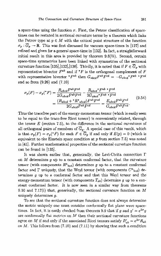
The Connection and Curvature Structure of Space- Time 281
a space-time using the function u. First, the Petrov classification of space- times can be restated in sectional curvature terms by a theorem which links the Petrov type at p E M with the critical point structure of the function cP : G, --j W. This was first discussed for vacuum space-times in [I271 and refined and given for a general space-time in [132]. In fact, a straightforward initial result in this area is provided by theorem 9.8(iii). Second, certain space-time symmetries have been linked with symmetries of the sectional curvature function [135],[132],[136]. Thirdly, it is noted that if F E cp with representative bivector Fab and if *F is the orthogonal complement of F with representative bivector *Fab then GabcdFabFCd = -Gabcd*Fab *Fed and so from (9.26) and (7.10)
-
(9.54)
Thus the tracefree part of the energy-momentum tensor (which is easily seen to be equal to the trace-free Ricci tensor) is conveniently related, through the tensor E (section 7.5), to the difference in the sectional curvatures of all orthogonal pairs of members of cp. A special case of this result, which is that up(F) = u p ( * F ) for each F E G, if and only if E(p) = 0 (which is equivalent to the Einstein space condition at p from section 7.5) was noted in [41]. Further mathematical properties of the sectional curvature function can be found in [135].
It was shown earlier that, generically, the Levi-Civita connection l? on M determines g up to a constant conformal factor, that the curvature tensor (with components Rabcd) determines g up to a constant conformal factor and r uniquely, that the Weyl tensor (with components Cab&) de- termines g up to a conformal factor and that this Weyl tensor and the energy-momentum tensor (with components T a b ) determine g up to a con- stant conformal factor. It is now seen in a similar way from theorems 9.10 and 7.17(i) that, generically, the sectional curvature function on M uniquely determines g.
To see that the sectional curvature function does not always determine the metric uniquely one must consider conformally flat plane wave space- times. In fact, it is easily checked from theorem 9.9 that if g and g‘ = e2ag are conformally flat metrics on M then their sectional curvature functions agree on M if and only if the associated Ricci tensors satisfy Rib = e2aRab on M . This follows from (7.10) and (7.11) by showing that such a condition

282 Symmetries and Curvature Structure in General Relativity
on the Ricci tensors forces all the conditions (i)-(vi) of theorem 9.9 to hold. Now let ( M , g ) be the plane wave space-time (8.11) with H = f(u)(z2+y2). A direct calculation of the Ricci tensor Rbb for ghb = e2u(u)gab in terms of the Ricci tensor Rab for gab (and noting that o , ~ = bea with u = 2 and ea;b = 0) shows that the condition Rhb = e2uRab is equivalent to the condition [129], [130] ,[136]
ii - u2 = f ( u ) ( l - e20) . (9.55)
Thus for a given plane wave one can always, at least locally, find metrics like 9’. An explicit solution of (9.55) is found [129],[130] by starting with
and choosing O ( U ) = e2u (8.11) with H as above for u > 0 and f(u) = ~
e2u - 1 - l e n ( e 2 ~ 2 - 1).
9.5 Retrospect
The interrelations between the metric, its associated Levi-Civita connection and the corresponding curvature structure have attracted many workers both in the purely mathematical aspects as well as those applicable to theoretical physics. For the case of a positive definite metric the problem of recovering a metric from its curvature tensor was considered by Kowalski [I371 whilst an early study of the same problem and which applied to general relativity theory was carried out by Ihrig [138],[139] who drew attention to the significance of equation (9.6) in this context. This work was followed up in [140] and led, through [118],[119], to the methods described in section 9.3. Further attention was given to this and related problems in [95] and [141]- [144]. The relationship between the metric and its associated connection studied in section 9.2 has been reconsidered in [145]-[148]. In the sectional curvature problem discussed in section 9.4 the contributing papers [I261 and [129],[130] were independent efforts. The present author was unaware of the work in [I291 when [126] was being written and is indebted to Professor Schimming in Greifswald for pointing it out to him and to Professor Voss in Zurich for sending him a copy of it. Some applications of the sectional curvature function together with a further bibliography can be found in
There is another rather interesting topic which is not unrelated in spirit to the work of this chapter. This is the so-called “equivalence problem” of Cartan [151] and others (and reviews of it can be found in [152],[153]). The
[ 1491, [ 1501.
The Connection and Curvature Structure of Space- Tame 283
application of this work to space-time manifolds has been actively pursued in the literature and involves significant use of computers. It will not be discussed any further here except to suggest the following references [154]- [157] for further reading.

This page intentionally left blank
Chapter 10
Affine Vector Fields on Space-Time
10.1 General Aspects of Symmetries
The remaining chapters of this book are concerned with symmetries in general relativity and this section will describe some general features of the mathematical study of such symmetries. The remainder of the chapter will concentrate on affine (including homothetic and Killing) symmetry. Throughout, M will be a space-time with (smooth) Lorentz metric g.
A symmetry of the space-time M , loosely speaking, is a smooth local diffeomorphism f : U --f V where U and V are open subsets (i.e. open submanifolds) of M which preserves some geometrical feature of M . If one requires such local symmetry everywhere on M one would require many such triples (each triple consisting of f , U and the geometrical feature preserved). This is usually achieved, not by specifying such triples, but by assuming the existence of a smooth vector field on M whose associated local diffeomorphisms and domains (section 5.11) together with the geometrical feature preserved play the role of such triples. If these local diffeomorphisms each satisfy the required symmetry condition then the associated vector field is regarded as a symmetry vector field (of the appropriate type). This concept of a “symmetry vector field” on M will be used throughout the remainder of this text. The details of which geometrical feature of M is to be preserved by the local diffeomorphisms will be described when required.
The symmetries to be discussed will constitute a real vector space S of global smooth vector fields on M (and usually S will be a Lie algebra under the Lie bracket operation). The clause that each member of S is global is largely for convenience. If they are not global and if the intersections of the domains of the members of S is a non-empty open subset U of M , then one could concentrate attention on the (components of the) open submanifold
285

286 Symmetries and Curvature Structure in General Relativity
U , thus effectively reinstating the global nature of these vector fields. The symmetries which will be discussed in this and subsequent chap-
ters are represented by vector fields whose associated local diffeomorphisms either
i) ii)
iii)
iv)
v) vi)
preserve geodesics (projective vector fields) or preserve geodesics together with their affine parameters (affine vector fields) or preserve the metric up to a conformal factor (conformal vector fields) or preserve the metric up to a constant conformal factor (homothetic vec- tor fields) or preserve the metric (Killing vector fields) or preserve some other fundamental part of space-time geometry, e.g. the curvature tensor.
A more precise definition of these symmetries will be given when re- quired. It is remarked here that a smooth vector field X is said to preserve a smooth tensor T on M if, for each smooth local diffeomorphism $t asso- ciated with X, the tensors T and &*T are equal on the domain U of d t . An equivalent statement is (section 5.13) that CxT = 0 on M . In fact if one chooses a coordinate domain V 2 U with coordinate functions xa then &(V) is also a coordinate domain of M with coordinates y a = xa o 4;'. Then at p E V
where q = g5t(p). Then from the definition of pullback and of tensor com- ponents (sections 4.7 and 4.9) one finds (writing Tq for T(q), etc)
Thus, quite generally, the components of &*T at p in the coordinate system xa equal the components of T at q in the coordinate system ya. Then if, in addition, dt is a symmetry of T , that is, 4,*T = T , then the components of T in V in the coordinates xa are pointwise equal (under q5t) to the
Afine Vector Fields on Space-Tame 287
components of T in +t(V) in the coordinates ya. This coordinate calculation is the justification for the equation C x T = 0 defining a symmetry vector field of T (and, roughly speaking, demands that the components of T are unaltered if the coordinate system is ‘carried along’ by X (ie. by the maps + t ) h
10.2 Affine Vector Fields
A global smooth vector field X on a space-time M is called an affine vector field (or an affine collineation) if each of the smooth local diffeomorphisms +t associated with X is an affine map, that is, each map $t preserves the geodesics of M and their affine parameters. Thus, with appropriate do- mains and ranges, if I is an open interval of R and c : I -+ M is an affinely parametrised geodesic of M then +t o c is also an affinely parametrised geodesic of M . There are two important results associated with an affine vector field X and its local diffeomorphisms &. First, the geodesic pre- serving property of $t shows that $t ‘commutes’ with the exponential map exp, at m E M in the sense that if m’ = +t(m) [20]
+t o exp, = expml O$t* (10.3)
This result says that the action of +t is mirrored in the tangent space by &* through the exponential maps at m and m’. It will be useful later. The second result involves the definition of the Lie derivative of the Levi-Civita connection V on M associated with the space-time metric g with respect to a smooth vector field X on M [158],[159]. It is denoted by CxV and acts on two vector fields Y and 2 on (some open subset U of) M , converting them to the vector field on U defined by
LXV(Y, 2) = [ X , VY 21 - V [ X , Y ] 2 - VY [X’ 21 (10.4)
It is easily checked that if f and g are smooth maps : U -+ R then L x V ( f Y , g Z ) = fgLxV(Y, 2). From this result, an argument similar to that given for the curvature tensor in section 4.16 shows that C x V leads to a type (1,2) tensor field on U with components in some coordinate system xa denoted by CFc and given by
(10.5)
2aa Symmetr ies and Curvature Structure in General Relativity
From the definitions of the Lie bracket and V one finds
ctc = X a ; b c - R a b c d X d (10.6)
Now the condition that X is affine can be shown equivalent 11591 (see also [20], [158]) to the condition LxV = 0 and hence, from (10.6), to
X a ; b c = R a b c d X d (10.7)
An alternative and useful way of rewriting (10.7) is first to decompose the covariant derivative of X into its self adjoint and skew-self adjoint parts. This leads to a symmetric tensor h and a skew-symmetric tensor F (called the affine bivector of X ) satisfying in each coordinate domain
X a ; b = f h a b -k F a b
hab = 2 x ( a ; b ) = L X g a b = h a , F a b = -Fba
On substituting this into (10.7) one finds
1 2hab;c -b Fab;c = R a b c d X d
Symmetrising on the indices a and b then gives the conditions
(2) habit = 0 (22) Fab;c = R a b c d X d
on h and F . Conversely suppose (lO.lO)(i) holds. Then
X a ; b c = Fab;c
and then the Ricci identity (4.33) on X gives
Fab;c - Fac;b = X d R d a b c
Permuting the indices a, b and c in (10.12) then gives
d Fba;c - Fbc;a = x Rdbac
Fcb;a - Fca;b = X d R d c b a
(10.8)
(10.9)
( 10.10)
(10.11)
(10.12)
( 10.13)
(10.14)
Adding the last three equations and using the curvature symmetry Ra[bcdl = 0 then easily leads to (lO.lO)(ii) and hence to (10.7). It follows that the condition (lO.lO)(i) is equivalent to the statement that X is an affine vector field and that the condition (lO.lO)(ii) on F follows automatically from (lO.lO)(i). From this condition on F it follows that F a b ; c X c = 0 and so F is parallely transported along the integral curves of X . It now easily follows
Afine Vector Fields on Space-Time 289
(see section 7.2) that the nature (spacelike, timelike, null or non-simple) of F is constant along such integral curves.
Regarding differentiability, so far an affine vector field has been assumed smooth. Suppose, however, X is C2. Then (10.7) shows, since the curva- ture tensor is smooth, that X must be C 3 and then that X is C4 and so on. Thus the assumption that an affine vector field is smooth is no more restrictive than (in fact, equivalent to) assuming it C2 as a consequence of the smoothness of the connection I?. The smoothness of h and F is then immediate from (10.8).
Now let X be an affine vector field on M . Then one may characterise this fact by the equations
These equations are constructed out of first order partial derivatives of the components of the quantities X , h and F together with the terms supplied by the geometry of M (i.e. g, r and the curvature). This observation is, in many ways, more useful than the “second order in X” original characteri- sation given in (10.7). An immediate use will be made of this now.
Suppose X and Y are two affine vector fields on M with X satisfying (10.8) and Y satisfying
( 10.16)
Suppose also that at m E M , X ( m ) = Y(m) , h(m) = H ( m ) and F ( m ) = G(m) (This is equivalent to X and Y and their first covariant derivatives agreeing at m, X ( m ) = Y(m) and V X ( m ) = VY(m)) . Now let c be a smooth curve in M defined on an interval ( - E , E ) (0 < E E R) and starting at m such that the tangent vector T( t ) to c is nowhere zero for t E (-E, E )
and such that the range of c lies in a coordinate domain of M (containing m). Then a contraction of (10.8) with T b and (10.10) with TC reveals a system of first order differential equations of the form
1 Ya;b = -Hab + G a b (Hab = Hba, Gab = -Gba) 2
( 10.17)
where Da,Cab and Dab depend only on X , h and F and on t through the (given) geometry of M . Similar remarks apply to Y. Now the theory of first order differential equations shows that if the (ordered) triple of quantities ( X , h , F ) is equal to the triple (Y, H , G) at some t o E (-6, E ) they will be equal on some open interval containing to. Also, if these triples differ at
290 Symmetries and Curvature Structure in General Relativity
some to E ( - E , E ) they will (by continuity) differ in some open interval containing to . Thus, since ( - E , E ) is connected and since these triples are equal at m = c(O), they agree for each t E (-6, E ) . It now follows by using the freedom in the choice of c that if these triples agree at some point of M they will agree in some open neighbourhood of that point (and clearly if they are not equal at some point of M they will differ in some open neighbourhood of that point). Thus, the points where these triples agree and where they disagree constitute disjoint open subsets of M , with the former not empty, and since M is connected it follows that X = Y on M . Thus an affine vector field X on M is uniquely determined by the values of X , h and F (or, alternatively, X and V X ) at some (any) point m of M . Another important result also follows from this argument. It is clear from (10.7) that the set (denoted by A(M)) of affine vector fields on M forms a real vector space. In fact A ( M ) is also a Lie algebra under the usual bracket operation for vector fields. This can be shown in several ways (see [20]) and is clear from a consideration of the local diffeomorphisms associated with the bracket of two members of A ( M ) (section 5.13). A direct proof in the present formalism can be obtained by letting X and Y be affine vector fields on M and let 2 = [ X , Y ] . Then in local coordinates Z" = Y a ; b X b - Xa;bYb. First one computes Za;b and finds its symmetric part Pab = Z(a;b). The idea then is to show that Pab;c = 0. This can be achieved after a little calculation during which it is useful to note that if Mab is a bivector then RabcdMbd is skew-symmetric in a and c and also that the Ricci identities on h and H yield
haeRebcd + hbeReacd = HaeRebcd + HbeReacd = 0 (10.18)
Finally, since the zero vector field on M is always affine and since any affine vector field X is uniquely determined by X ( m ) , h(m) and F ( m ) at any m E M it follows that if these three quantities vanish for any m then X is identically zero on M . Thus the taking of linear combinations and a simple counting procedure shows that A ( M ) is finite dimensional and that dimA(M) < 4+ 10+6 = 20. The set A(M) will be referred to as the affine algebra of M .
The following theorem has thus been proved.
Theorem,lO.l vector fields on M .
Let M be a space-time and let A ( M ) be the set of afine
a) Each member X of A ( M ) satisfies (10.7) and (lO.lO)(i) and either of these conditions is suficient t o ensure that X is afine.
A f i n e Vector Fields on Space-Time 29 1
i i) Each member X of A(M) is uniquely determined by specifying the quan- tities X ( m ) , h(m) and F ( m ) or, alternatively, X ( m ) and V X ( m ) at any m E M (and hence if an af ine vector field vanishes over a non-empty open subset of M it vanishes everywhere on M)
iii) A(M) is a finite-dimensional Lie algebra of smooth vector fields on M under the Lie bracket operation and dimA(M) < 20. (For a connected n-dimensional manifold M with a linear connection dim A(M) 6 n(n + 1) I2014
The upper bound of 20 in part (iii) of theorem 10.1 is achieved in Minkowski space-time (and, as will be seen later, this is essentially the only way it is achieved). For in Minkowski space-time, (10.7) yields X a $ c = 0 for the components of an affine vector field in the usual global coordinate system. This is readily solved, the general solution being that each component X a is a general linear function of the coordinates
where xa = ( t , x, y , z ) are the usual Minkowski coordinates and the p a b
and Pa are 20 constants with the symmetric and skew-symmetric parts of Pab ZF qacPCb playing the role of hat, and Fab, respectively.
10.3 Subalgebras of the Affine Algebra; Isometries and Ho- mothet ies
The affine algebra A(M) of a space-time M has some important subal- gebras. The two which are, perhaps, the most important in the present context are the Killing and homothetic subalgebras and these can now be discussed.
Let X E A(M) so that X is an affine vector field on M. Then X satisfies (10.8) and the affine condition is the condition that h is covariantly constant. If h = 0 on M then X satisfies the equivalent conditions
This equation is called Killing's equation and the vector field X is then called a Killing vector field. The associated bivector F will be called the
292 Symmetries and Curvature Stmcture in General Relativity
Killing bivector (of X ) . The subset of A ( M ) consisting of all Killing vector fields on M will be called the Killing algebra and is denoted by K ( M ) .
Now suppose X E A ( M ) and in the resulting equation (10.8) h = 2cg on A4 where c is a (constant) real number. Then X satisfies the equivalent conditions
and is called a homothetic vector field. The associated bivector F is then called the homothetic bivector and c the homothetic constant (of X ) . The subset of A ( M ) consisting of all homothetic vector fields on M will be referred to as the homothetic algebra and denoted by H ( M ) . A consideration of the case c = 0 shows that K ( M ) C H(A4). If X E H ( M ) and the corresponding constant c # 0 then X is called proper homothetic. For later convenience it will be assumed that if X is proper homothetic then (by changing X to -X if necessary) c > 0. If X E A ( M ) is neither Killing nor homothetic it is called proper affine. The subsets of proper affine and proper homothetic vector fields are not subspaces of A ( M ) .
The definitions of affine, Killing and homothetic vector fields given in (lO.lO), (10.20) and (10.21) apply quite generally for manifolds (where they make sense) and will, on occasions, be used for manifolds other than space- times together with the obvious appropriate notation.
If one refers to the collection of results regarding the Lie derivative given in section 5.13 it is clear that if X , Y and 2 = ax +BY E A ( M ) , a, p E R, then Lxg = Lyg = 0 + Czg = C[x,y]g = 0 and Lxg = 2clg, .cYg = 2c2g + Czg = 2c3g and C[x,y]g = 0 where c1, c2 and c3 (= ac1 + pc2) are constants. It follows that K ( M ) and H ( M ) are each Lie subalgebras of A ( M ) and that K ( M ) is a Lie subalgebra of H ( M ) ) . Also any X E K ( M ) is uniquely determined by the values X ( m ) and F ( m ) at some (any) m E M (since, then h(m) = 0 is necessarily true) and any X E H ( M ) is uniquely determined by the values X ( m ) , F ( m ) and the constant c (since, then h(m) necessarily equals cg(m)). These results follow from theorem 10.1. One can now collect these results (and more) together in the following theorem.
Theorem 10.2 homothetic algebra H(A4).
Let M be a space-time with Killing algebra K ( M ) and
i) The members of K ( M ) are characterised by their satisfying equation (10.20) and each X E K ( M ) is uniquely determined by the valuesX(m)
A f i n e Vector Fields on Space-Time 293
and F ( m ) at any m E M .
i i ) T h e members of H ( M ) are characterised by their satisfying the equa- t ion (10.21) and each X E H ( M ) is uniquely determined by the values X ( m ) , F ( m ) and c at any m E M .
iii) The Lie algebras K ( M ) and H ( M ) are finite-dimensional Lie algebras of smooth vector fields o n M . K ( M ) and H ( M ) are subalgebras of A ( M ) and K ( M ) i s a subalgebra of H ( M ) . Further, dimK(M) f 10, dimH(M) 6 11 and dimH(M) 6 dimK(M) + 1 . ( h fact in the gen- eral case of a n n-dimensional manifold M admitting a metr ic of any signature, dimK(M) 6 in(n + 1) and dimH(M) 6 in(n + 1) + 1.)
i v ) I f X , Y E H ( M ) , [ X , Y ] E K ( M ) .
Regarding the upper bounds on the dimensions in part (iii) of this theorem it is a classical result (see, e.g. 1351 and the final paragraph of this chapter) that if dimK(M) = $n(n+l) (= 10 for a space-time) then M has constant curvature and that if M has constant curvature then M admits a local Killing algebra of dimension $n(n+l) in the sense that each m E M admits a connected open neighbourhood U such that U with induced metric from g on M satisfies dimK(U) = an(.+ 1). For example, in Minkowski space- time, one can solve Killing's equation by imposing (10.20) on the f i n e solution (10.19) for Minkowski space. The result is
xa = Pa6lCb + pa Pab + Pba = 0 Pa6 = q a c P c b (10.22)
and the 6 + 4 = 10 independent constants in pa6 and Pa show the Killing algebra to have dimension 10. It will be shown later that if dimK(M) > 7 then M has constant curvature and that dimK(M) # 9 (see end of chapter). If dimH(M) = 11 then, as will also be seen later, M is flat and a flat space-time always admits an 1 l-dimensional local homothety algebra (in the same sense as the above local Killing algebra), since Minkowski space-time does, namely the vector fields in (10.22) together with the proper homothetic vector field X with components X a = (t , 5, y , z) . Similar results apply in an obvious way to manifolds of any dimension and which admit a metric.
For the last inequality in part (iii) one notes that since K ( M ) is a sub- space of H ( M ) , dimK(M) = dimH(M) if and only if K ( M ) = H ( M ) . If K ( M ) # H ( M ) then there exists a proper homothetic vector field X

294 Symmetries and Curvature Structure in General Relativity
satisfying Lxg = 2cg with c a non-zero constant. If Y is any other ho- mothetic vector field satisfying C y g = 2c’g for some non-zero constant c‘ then 2 = c’X - CY satisfies Lzg = 0 and so 2 is Killing. Hence Y = c’c-lX - c-lZ may be written as a linear combination of the origi- nal homothetic vector field X and a Killing vector field. It follows in this case that dim H ( M ) = dim K ( M ) + 1 because a basis for K ( M ) augmented with X is a basis for H ( M ) . Part (iv) follows immediately from the remarks preceding the theorem.
The geometrical interpretation of an affine vector field arises from the fact that the corresponding local diffeomorphisms +t preserve the geodesics and their affine parameters. In fact they preserve the connection r as can be made precise in an elegant way [20]. This latter fact can also be demonstrated at an elementary level by considering one such local affine transformation dt whose domain U is a coordinate neighbourhood with coordinates xa. Then +t is smooth (since X is) and so (section 10.1) V = +t(U) can be considered a coordinate domain of M with coordinates ya = xa o $I;’, The geodesic property of +t can now easily be used to see that the connection coefficients J?Ec in U in the xu coordinates are equal, pointwise under +t, to the coefficients I’k in V in the ya coordinates. This should be compared to a similar argument for symmetries of tensors given in section 10.1.
The geometrical interpretation for a Killing vector field X on M arises from the condition Lxg = 0 and hence $t*g = g (section 10.1 with T = g) for each local diffeomorphism +t associated with X. Hence each +t is a local symmetry of the metric g.
If X is a homothetic vector field on M one has Cxg = 2cg with c constant and so (section 5.13) each associated local diffeomorphism +t of X satisfies &*g = ezctg. Thus each given +t is a dilatation of the metric g.
The existence of an affine, Killing or homothetic vector field on M leads to a family of special coordinate systems on M . Let X be a Killing vector field on M and suppose that m E M and X(m) # 0. Then from theorem 4.12 there exists a coordinate domain U containing m with coordinates xa such that, in U , X = &. Now Killing’s equation (10.20) can be rewritten from (5.13) as
gab,cXc + gacXc,b + gbcXc,a = 0 (10.23)
which in the above coordinates on U gives % = 0 and so the metric corn- ponents are, in this coordinate system, independent of the coordinate xl . A similar argument with the above coordinate system when X (=&) is a
Afine Vector Fields on Space-Time 295
homothetic vector field satisfying (10.21) shows that = 2Cgab and so gab = e2cx'qab where the qab are independent of x1 (and gab is a Lorentz metric on U for which X is Killing). The geometrical interpretation of an affine vector field given above shows that when X is an affine vector field then, in the above coordinate system the coefficients rtc are independent of xl. Conversely, suppose that in some coordinate domain U with coordi- nates Z" the metric components are independent of xl. Then from (10.20), X = & is a Killing vector field on U . Similarly if the metric components satisfy gab = ezCx'qab for some constant c and where the qab are independent of x1 then X = & is a homothetic vector field on U and, again, if the co- efficients J?& are independent of x1 then X = & is an affine vector field on U . The extension of these results to several independent vector fields of the appropriate type is clear from theorem 4.12. Thus if X I , . . . , XN E K ( M ) and none vanishes at m E M and [Xi,Xj] = 0 (1 6 i , j < N ) then there is a coordinate domain about m in which X1 = A, ~9 , X N = and gab is independent of xl,. . . , xN and, conversely, if gab is independent of XI,. . , xN, G,. . . , & are Killing vector fields on the coordinate domain (and the Lie bracket of any two of them vanishes). Similar results hold for H ( M ) and A ( M ) (where, if &,. .. , & are homothetic with homoth- etic constants c1 . ' , CN, gab = e 2c" ' f~~+2cNxNpab with pab independent of
It is useful to note that if X is a homothetic vector field on M satisfying (10.21) and if a = g(X, X ) (in components a = X"X,) then it follows that
a
a
. . ,xN).
g , , x a = 2ca (10.24)
Now if m E M and X(m) = 0 the integral curve of X through m is a constant map with range {m}. If, however, X(m) # 0 then (10.24) shows that along any integral curve of X through m with parameter t ,
= 2ca. It follows that the nature (spacelike, timelike or null) of X is constant along its integral curves and that along such curves, a is constant if X E K ( M ) . The same result is not true for a proper f i n e vector field, a counterexample coming from (10.19) by considering the proper affine vector field X a = ( t , 1,0,0) in Minkowski space. Also, if X E H ( M ) and fX E H ( M ) with f : M + W then it is easily checked that f is necessarily constant. Again this result is not true for A ( M ) as the affine vector fields X" = (1,0,0,0) and t X a in Minkowski space show.
The situation will occasionally arise when the idea of a local symmetry (vector field) is required. This is defined to be a vector field of a type
296 Symmetries and Curvature Stmcture in General Relativity
discussed so far, or still to be introduced, but which is defined on an open subset U of M .
10.4 Fixed Point Structure
Let X be a non-trivial &ne vector field on the space-time M and suppose m E M . If X ( m ) = 0 then m is a fixed point or a zero of X . The term fixed point arises since, if $t is a local diffeomorphism associated with X , q$ (m) = m, and so m is a fixed point of any such $Jt . If U is a coordinate neighbourhood of such a zero m with coordinates ya then the vector space isomorphism &* : T,M -+ T,M is represented in the basis (&)m by the transpose of the matrix [21] (see 5.9)
axb exp tA = exp t ( F )
m (10.25)
where A, with components ( g ) m , is the linearisation of X at m. The need to transpose this matrix is to conform to the fact that a different definition of the matrix of a linear transformation is taken here (chapter 2) from that in [21]. F'rom (10.8) it follows that A has components Aab = (ih"b + Fab) (m) and from (10.3) that if exp, is the usual exponential diffeomorphism from some open neighbourhood of 0 E T,M onto some open neighbourhood V of m then
In the normal coordinate system xa with domain V resulting from the basis (&) (= (&),) of TmM the integral curves of X satisfy = Aabxb. This follows because if q E V , the integral curve t 4 &(q) of X through q is t 4 4tOexpm(q') = exp, 04t*(q') = exP,(q'(exptA)*) = exp,((exptA)q') where exp, q' = q. Then use property (v) following theorem 5.4. F'rom this it follows that in this coordinate system the components of X are linear functions of the coordinates, X a = Aabxb. A vector field X is called lineaxis- able about m if, in some coordinate neighbourhood of m, the components X a of X are linear functions of the coordinates. By theorem 4.12(i) this is true for any vector field X if X ( m ) # 0. The above shows that any affine vector field on M is linearisable about any point of M . This property which follows from the fact that the maps q5t preserve geodesics and their &ne parameters is useful. For example, the set of zeros of X lying in the
m
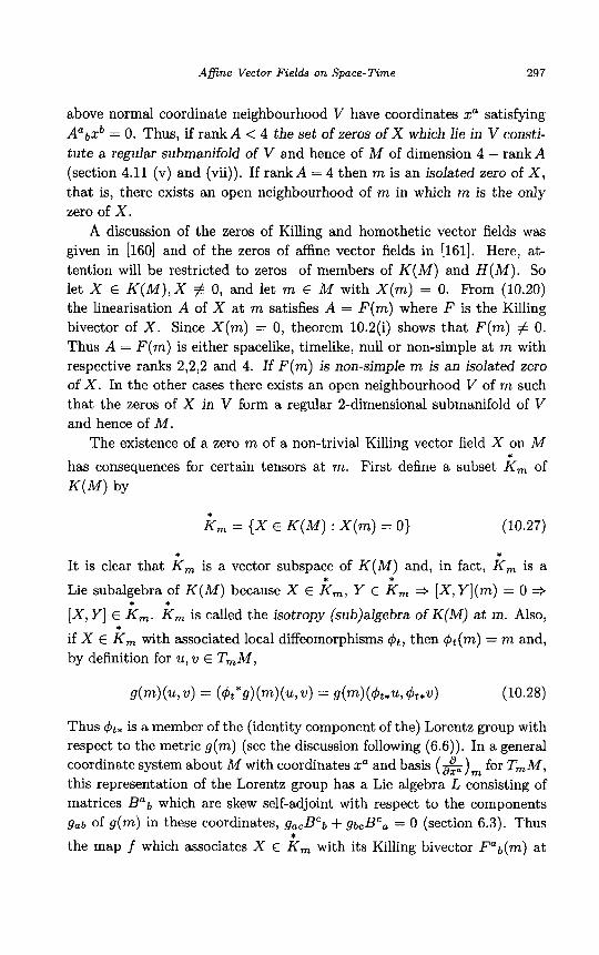
A f i n e Vector Fields on Space-Time 297
above normal coordinate neighbourhood V have coordinates xa satisfying Aabxb = 0. Thus, if rank A < 4 the set of zeros of X which lie in V consti- tute a regular submanifold of V and hence of M of dimension 4 - rankA (section 4.11 (v) and (vii)). If rankA = 4 then m is an isolated zero of X , that is, there exists an open neighbourhood of m in which m is the only zero of X .
A discussion of the zeros of Killing and homothetic vector fields was given in [160] and of the zeros of f i n e vector fields in [161]. Here, at- tention will be restricted to zeros of members of K ( M ) and H ( M ) . So let X E K ( M ) , X $ 0, and let m E M with X ( m ) = 0. €+om (10.20) the linearisation A of X at m satisfies A = F ( m ) where F is the Killing bivector of X . Since X ( m ) = 0, theorem 10.2(i) shows that F ( m ) # 0. Thus A = F ( m ) is either spacelike, timelike, null or non-simple at m with respective ranks 2,2,2 and 4. If F ( m ) is non-simple m is an isolated zero of X . In the other cases there exists an open neighbourhood V of m such that the zeros of X in V form a regular 2-dimensional submanifold of V and hence of M .
The existence of a zero m of a non-trivial Killing vector field X on M has consequences for certain tensors at m. First define a subset K , of K ( M ) by
* K , = { X E K ( M ) : X ( m ) = 0) (10.27)
It is clear that K , is a vector subspace of K ( M ) and, in fact, K , is a
Lie subalgebra of K ( M ) because X E K,, Y E Km + [ X , Y ] ( m ) = 0 + [X, Y ] E K,. K , is called the isotropy (sub)algebra of K(M) a t m. Also,
if X E K , with associated local diffeomorphisms +t, then +t(m) = m and, by definition for u, u E T,M,
* *
* * * *
*
Thus & is a member of the (identity component of the) Lorentz group with respect to the metric g(m) (see the discussion following (6.6)). In a general coordinate system about M with coordinates x a and basis (&) for T,M, this representation of the Lorentz group has a Lie algebra L consisting of matrices Bab which are skew self-adjoint with respect to the components gab of g ( m ) in these coordinates, gacBCb + gbcBCa = 0 (section 6.3). Thus the map f which associates X E K , with its Killing bivector Fab(m) at
*
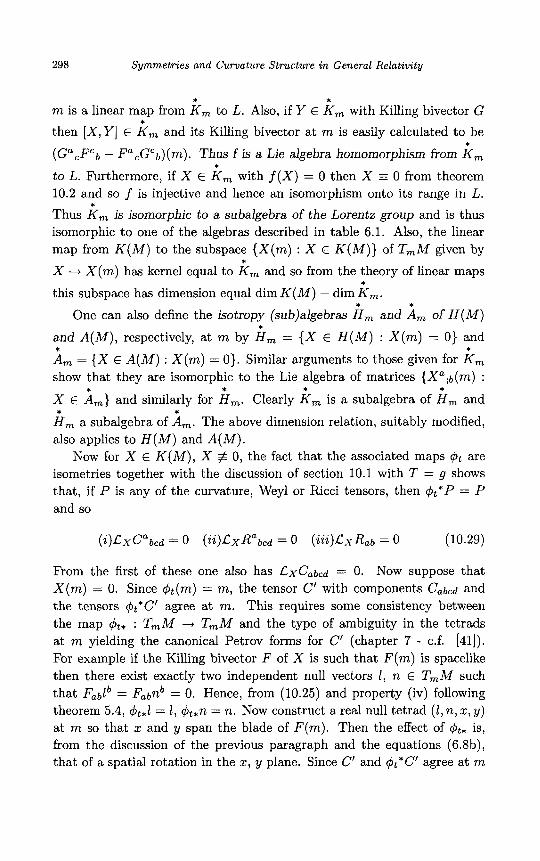
298 Symmetries and Curvature Stmcture in General Relativity
* * m is a linear map from K , to L. Also, if Y E K , with Killing bivector G then [ X , Y ] E K , and its Killing bivector at m is easily calculated to be
*
(GacFCb - FacGcb)(m). Thus f is a Lie algebra homomorphism from K,
to L. Furthermore, if X E K, with f ( X ) = 0 then X = 0 from theorem 10.2 and so f is injective and hence an isomorphism onto its range in L. Thus K , is isomorphic to a subalgebra of the Lorentz group and is thus isomorphic to one of the algebras described in table 6.1. Also, the linear map from K(M) to the subspace { X ( m ) : X E K ( M ) } of T,M given by
X -+ X ( m ) has kernel equal to K , and so from the theory of linear maps
this subspace has dimension equal dimK(M) - dim K,.
*
*
* *
* * One can also define the isotropy (sub)algebras H, and A, of H(M)
and A(M), respectively, at m by H, = { X E H(M) : X ( m ) = 0) and
A, = { X E A(M) : X ( m ) = 0). Similar arguments to those given for K , show that they are isomorphic to the Lie algebra of matrices {X";b(m) :
X E A,} and similarly for H,. Clearly K , is a subalgebra of H , and
H , a subalgebra of A,. The above dimension relation, suitably modified, also applies to H(M) and A(M).
Now for X E K(M), X $ 0, the fact that the associated maps q5t are isometries together with the discussion of section 10.1 with T = g shows that, if P is any of the curvature, Weyl or Ricci tensors, then $t*P = P and so
*
* *
* * * * * *
From the first of these one also has LxCabcd = 0. Now suppose that x ( m ) = 0. Since q!Jt(m) = m, the tensor c' with components Cabcd and the tensors $t*C' agree at m. This requires some consistency between the map & : T,M -+ T,M and the type of ambiguity in the tetrads at m yielding the canonical Petrov forms for C' (chapter 7 - c.f. [41]). For example if the Killing bivector F of X is such that F ( m ) is spacelike then there exist exactly two independent null vectors 1 , n E T,M such that Fablb = Fabnb = 0. Hence, from (10.25) and property (iv) following theorem 5.4, & I = I , &*n = n. Now construct a real null tetrad ( I , n, x, y) at m so that x and y span the blade of F ( m ) . Then the effect of dt* is, from the discussion of the previous paragraph and the equations (6.8b), that of a spatial rotation in the x, y plane. Since C' and &*C' agree at m

A f i n e Vector Fields on Space-Time 299
one finds that the components Cab& are the same in the frames (1, n, x, y) and (1, n, &x, &y). It also follows that since C , if non-zero at m, admits a finite number of principal null directions, the continuity of &* means that each principal null direction must be preserved by &. Since & is a Lorentz transformation there are at most two principal null directions (either 1, n or both). Thus (chapter 7) the Petrov type is either N, 111, D or 0. Reference to the discussion of Petrov tetrads at the end of section 7.3 yields a contradiction in the type N and I11 cases and so C must have type D or 0 at m with 1 and n spanning the (necessarily repeated) principal null directions of C in the type D case. A similar argument and conclusion follow if F(m) is timelike or non-simple. If F(m) is null one can find a null tetrad ( l ,n ,x ,y) such that Fablb = Fabyb = 0 at m and so (bt*l = 1, qhtly = y and with &+ yielding a null rotation in the 1,x plane (equation (6.8d). Since 1 spans the unique null direction preserved by the &, at most one principal null direction of the Weyl tensor at m is now permitted. Thus the Petrov type at m is N or 0 with 1 spanning the (necessarily repeated) principal null direction in the type N case.
Now consider the Ricci tensor, Ricc, and the third equation in (10.29). One now has that Ricc and &* Ricc agree at m. Now the condition that k is an eigenvector of Ricc at m with eigenvalue p E C is equivalent to the condition that Ricc(k, k’) = pg(k, k’), Vk’ E T,M. So
Since $t* is an isomorphism of T,M it follows that q5t- k is also an eigenvec- tor of Ricc with eigenvalue p. This produces degeneracies in the algebraic structure of Ricc depending on the nature of &, that is, on F(m). The individual details can be read off from the possible Segre types for Ricc in chapter 7 ([160], [162], [ 5 5 ] ) . They are given in table 10.1. An alternative proof here follows by noting that (10.29)(iii) applied at m is
RacFCb + RbcFCa = 0 (10.31)
The same results can now be read off from theorem 9.1 replacing the tensor g’ there by Ricc. The following theorem can now be stated.
Theorem 10.3 Let X be a non-trivial Killing vector field on a space- time M which has a zero at m € M and let F be the Killing bivector of X . Then F(m) # 0 and the following hold.
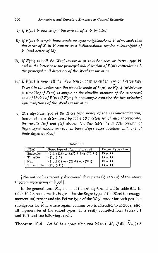
300 Symmetries and Curvature Stmcture in General Relativity
’ F(m) Segre type of Rab or Tab a t M {1,1, (11)) or (zZ(11)) or {2(11))
{(1,11)1} or {(21)1} or ((31))
Spacelike Timelike {(1,1)11} Null Non-simple {(1,1)(11)}
i) If F(m) i s non-simple the zero m of X i s isolated.
Petrov Type a t m D or 0 D or 0 N or 0 D or 0
ii) If F(m) is simple there exists a n open neighbourhood V of m such that the zeros of X in V constitute a 2-dimensional regular submanifold of V (and hence of M).
iii) If F(m) i s null the Weyl tensor at m is either zero or Petrov type N and in the latter case the principal null direction of F ( m ) coincides with the principal null direction of the Weyl tensor at m.
iv) If F(m) is non-null the Weyl tensor at m i s either zero or Petrov type
D and in the latter case the timelike blade of F(m) or F(m) (whichever i s timelike) if F(m) is simple or the timelike member of the canonical pair of blades of F(m) zf F(m) i s non-simple contains the two principal null directions of the Weyl tensor at m.
*
v) The algebraic type of the Ricci (and hence of the energy-momentum) tensor at m is determined by table 10.1 below which also incorporates the results (iii) and (iv) above. ( In this table the middle column of Segre types should be read as those Segre types together with any of their degeneracies.)
[The author has recently discovered that parts (i) and (ii) of the above theorem were given in [163].]
In the general case, K , is one of the subalgebras listed in table 6.1. In table 10.2 a complete list is given for the Segre type of the Ricci (or energy- momentum) tensor and the Petrov type of the Weyl tensor for each possible
subalgebra for K,, where again, column two is intended to include, also, all degeneracies of the stated types. It is easily compiled from tables 6.1 and 10.1 and the following result.
Theorem 10.4
*
*
* Let M be a space-time and let m E M , If dimK, 2 3
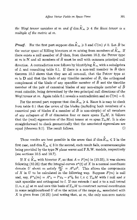
A f i n e Vector Fields on Space-Time 30 1
* the Weyl tensor vanishes at m and if dimK, 2 4 the Ricci tensor is a multiple of the metric at m.
Proof. For the first part suppose d i rn i , 2 3 and C(m) # 0. Let B be
the vector space of Killing bivectors at m arising from members of K,. If there exists a null member of B then, from theorem 10.3, the Petrov type at m is N and all members of B must be null with common principal null
direction. A contradiction now follows by identifying K, with a subalgebra of L and consulting table 6.1. If there is a non-null member in B then theorem 10.3 shows that they are all non-null, that the Petrov type at m is D and that the blade of any timelike member of B, the orthogonal complement of the blade of any spacelike member of B and the timelike member of the pair of canonical blades of any non-simple member of B must coincide, being determined by the two principal null directions of the Weyl tensor at m. Again table 6.1 reveals a contradiction and so C(m) = 0.
*
*
* - For the second part suppose that dim K , 2 4. Since it is easy to check
from table 6.1 that the union of the blades (including both members of a canonical pair of blades if a member of B is non-simple) of all members of any subspace of B of dimension four or more spans T,M, it follows that the (real) eigenvectors of the Rcci tensor at m span T,M. It is also straightforward to check geometrically that the associated eigenvalues are
0 equal (theorem 9.1). The result follows.
* These results are best possible in the sense that if dim K, < 2 in the
first case, and dim K , 6 3 in the second, each result fails, counterexamples being provided by the type N plane waves and F.R.W. models, respectively (see sections 10.5 and 10.7).
If X E K, with bivector F , so that A = F ( m ) in (10.25), it was shown following (10.26) that the integral curves xa( t ) of X in a normal coordinate domain U about m satisfy = Aabxb. This allows the components of X in U to be calculated in the following way. Suppose F ( m ) is null and, say, Fab(m) = Aab = laxb - xalb for 1,x E T,M with 1 null and x unit spacelike and orthogonal to 1. If one extends 1 and x to a null tetrad ( 1 , n, x , y) at m and uses this basis of TmM to construct normal coordinates in some neighbourhood U of m the action of the maps q5t* associated with X is given from (10.25) (and noting that, at m, the only non-zero metric
8
*
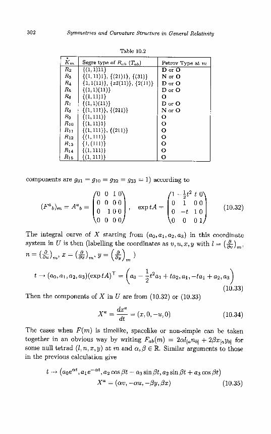
302 Symmetries and Curvature Structure in General Relativity
Table 10.2
Petrov Type at m D or 0 N or 0 D or 0 D or 0 0 D or 0 N or 0 0 0 0 0 0 0 0
components are go1 = 910 = g22 = g33 = 1) according to
0 0 1 0
0 - 1 0 0 0 -t 1 0 0 0 0 0 0 0 0 1
1 -;t2 t 0 (Fag)m=Aab= ( 0 0 0 0 ) , exptA= ( 0 1 0 0 ) (10.32)
The integral curve of X starting from (aola1,a2,a3) in this coordinate system in U is then (labelling the coordinates as w, u, x, y with 1 = ( & ) m ,
a a
t 4 ( a o , a l , a z , a 3 ) ( e ~ p t A ) ~ = +ta2,al,-tal +a2,a3
(10.33) Then the components of X in U are from (10.32) or (10.33)
(10.34)
The cases when F ( m ) is timelike, spacelike or non-simple can be taken together in an obvious way by writing F,g(m) = 2alianb] + 2,Bx[,ybl for some null tetrad (I, n, x, y) at m and a, P E R. Similar arguments to those in the previous calculation give
t + (aOeQt, ale-at, a2 cospt - a3 sin Pt, a2 sin Pt + a3 cos Pt)
X" = (aw, -au, -by, Px) (10.35)
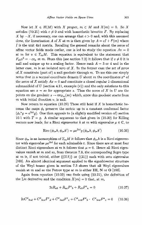
Afine Vector Fields on Space-Time 303
Now let X E H ( M ) with X proper, m E M and X(m) = 0. So X satisfies (10.21) with c # 0 and with homothetic bivector F . By replacing X by - X , if necessary, one can arrange that c > 0 and, with this assumed done, the linearisation A of X at rn is then given by A = c1 + F(m) where I is the unit 4x4 matrix. Recalling the general remarks about the zeros of affine vector fields made earlier, one is led to study the equation Av = 0 at m for v E T,M. This equation is equivalent to the statement that F,bVb = -ma at m. From this (see section 7.2) it follows that if v # 0 it is null and unique up to a scaling factor. Hence rank A = 3 or 4 and in the latter case, m is an isolated zero of X. In the former case the set of zeros of X constitute (part of) a null geodesic through m. To see this one simply notes that in a normal coordinate domain U about m the coordinates xa of the zeros of X satisfy Ax = 0 and constitute a closed regular 1-dimensional submanifold of U (section 4.11, example (v)) and the only solutions to this equation are x = sv for appropriate s. Thus the zeros of X in U are the points on the geodesic s + exp,(sv) which, since this geodesic starts from m with initial direction v, is null.
Now return to equation (10.29) These still hold if X is homothetic be- cause the maps $t preserve the metric up to a constant conformal factor (&*g = eactg). One then appeals to (a slightly modified version of) section 10.1 with T = g . A similar argument to that given in (10.30) for Killing vectors now leads, for a Ricci eigenvector Ic at m with eigenvalue p E C, to
RCC ($t*k, $t*k’) = peactg ($t*IC, $t*k’) (10.36)
Since &+ is an isomorphism of T,M it follows that &Ic is a Rcci eigenvec- tor with eigenvalue pe2ct for each admissible t . Since there are at most four distinct Ricci eigenvalues at m it follows that p = 0. Hence all Ricci eigen- values vanish at m and so, from theorem 7.8, the corresponding Segre type at m is, if not trivial, either ((211)) or ((31)) each with zero eigenvalue [l60]. An almost identical argument applied to the eigenbivector structure of the Weyl tensor given in section 7.3 shows that all Weyl eigenvalues vanish at m and so the Petrov type at m is either 111, N or 0 [160].
Again from equation (10.29) one finds using (10.21), the definition of the Lie derivative and the condition X(m) = 0 that, at m,
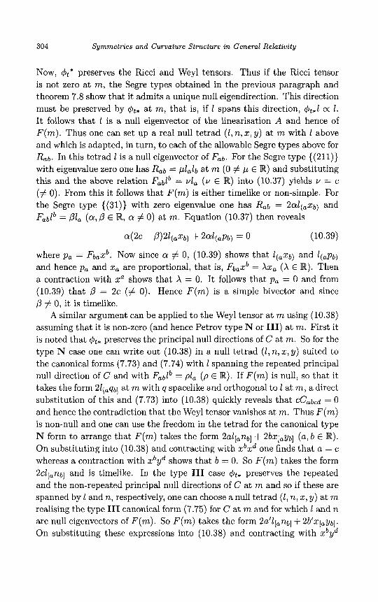
304 Symmetries and Curvature Structure in General Relativity
Now, $t* preserves the Ricci and Weyl tensors. Thus if the Ricci tensor is not zero at m, the Segre types obtained in the previous paragraph and theorem 7.8 show that it admits a unique null eigendirection. This direction must be preserved by & at m, that is, if 1 spans this direction, &*l c( 1. It follows that 1 is a null eigenvector of the linearisation A and hence of F ( m ) . Thus one can set up a real null tetrad ( l , n , x , y ) at m with 1 above and which is adapted, in turn, to each of the allowable Segre types above for Rab. In this tetrad 1 is a null eigenvector of Fab. For the Segre type ( (211)) with eigenvalue zero one has R,b = @alb at m (0 # p E R) and substituting this and the above relation = vl, (v E R) into (10.37) yields v = c (# 0) . From this it follows that F ( m ) is either timelike or non-simple. For the Segre type ((31)) with zero eigenvalue one has R,b = 2 d ( , X b ) and F,blb = pl, (a,P E R, a # 0) at m. Equation (10.37) then reveals
a(2c - p)21(axb) + 2al(apb) = 0 (10.39)
where pa = Fbaxb. Now since a # 0, (10.39) shows that l( ,Xb) and l(&) and hence pa and xa are proportional, that is, Fbaxb = Ax, (A E R). Then a contraction with xa shows that A = 0. It follows that pa = 0 and from (10.39) that p = 2c (# 0) . Hence F ( m ) is a simple bivector and since ,B # 0, it is timelike.
A similar argument can be applied to the Weyl tensor at m using (10.38) assuming that it is non-zero (and hence Petrov type N or 111) at m. First it is noted that & preserves the principal null directions of C at m. So for the type N case one can write out (10.38) in a null tetrad (1, n, x , y ) suited to the canonical forms (7.73) and (7.74) with 1 spanning the repeated principal null direction of C and with F,blb = pl, ( p E R). If F ( m ) is null, so that it takes the form 21[,qb] at m with q spacelike and orthogonal to 1 at m, a direct substitution of this and (7.73) into (10.38) quickly reveals that CC&d = 0 and hence the contradiction that the Weyl tensor vanishes at m. Thus F ( m ) is non-null and one can use the freedom in the tetrad for the canonical type N form to arrange that F ( m ) takes the form 2al[,nb] + 2bX[.yb] (a , b E W ) . On substituting into (10.38) and contracting with xbxd one finds that a = c whereas a contraction with xbyd shows that b = 0. So F ( m ) takes the form k l [ , n b ] and is timelike. In the type 111 case $t* preserves the repeated and the non-repeated principal null directions of C at m and so if these are spanned by 1 and n, respectively, one can choose a null tetrad (1, n, x , y ) at m realising the type I11 canonical form (7.75) for C at m and for which 1 and n are null eigenvectors of F ( m ) . so F ( m ) takes the form 2a’l[,nb] + 2b’x[,yb]. On substituting these expressions into (10.38) and contracting with xbyd
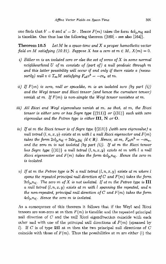
A f i n e Vector Fields on Space-Time 305
one finds that b' = 0 and a' = 2 c . Hence F(m) takes the form 4cl[,nbl and is timelike. One thus has the following theorem ([I601 - see also [164]).
Theorem 10.5 Let M be a space-time and X a proper homothetic vector field o n M satisfying (10.21). Suppose X has a zero at m E M , X(m) = 0.
i ) Either m is an isolated zero or else the set of zeros of X in some normal neighbourhood U of m consists of (part of) a null geodesic through m and this latter possibility will occur if and only i f there exists a (neces- sarily) null v E T, M satisfying FabVb = -cv, at m.
ii) If F(m) is zero, null or spacelike, m is an isolated zero (by part (a)) and the Weyl tensor and Ricci tensor (and hence the curvature tensor) vanish at m. If F(m) is non-simple the Weyl tensor vanishes at m.
iii) All Ricci and Weyl eigenvalues vanish at m, so that, at m, the Ricci tensor i s either zero or has Segre type ( ( 2 1 1 ) ) or ( ( 3 1 ) ) each with zero eigenvalue and the Petrov type is either 111, N or 0.
iv) If at m the Ricci tensor is of Segre type ( ( 2 1 1 ) ) (with zero eigenvalue) a null tetrad ( 1 , n, x , y ) exists at m with 1 a null Ricci eigenvctor and F(m) takes the form 2c~[,nb] + 2dx[,yb] (d E R). Hence, at m, Fabnb = - m a ,
and the zero m is not isolated (by part (a)). If at m the Ricci tensor has Segre type ( ( 3 1 ) ) a null tetrad ( l ,n ,x , y ) exists at m with 1 a null Ricci eigenvector and F(m) takes the form 4cl[,nbl. Hence the zero m is isolated.
v) If at m the Petrov type i s N a null tetrad (l,n,x, y ) exists at m where 1 spans the repeated principal null direction of C and F(m) takes the f o r m 2cl[,nb]. The zero m of X is not isolated. If at m the Petrov type is I11 a null tetrad ( l ,n ,x , y ) exists at m with 1 spanning the repeated, and n the non-repeated, principal null direction of C and F(m) takes the fo rm 4cl[,nbl. Hence the zero m is isolated.
As a consequence of this theorem it follows that if the Weyl and Ricci tensors are non-zero at m then F(m) is timelike and the repeated principal null direction of C and the null Ricci eigendirection coincide with each other and with one of the principal null directions of F(m) (spanned by 1 ) . If C is of type I11 at m then the two principal null directions of C coincide with those of F(m). Thus the possibilities at m are either (i) the

306 Symmetries and Curvature Structure in General Relativity
Ricci tensor is zero or has Segre type ((211)) with zero eigenvalue and the Weyl tensor is either zero or of Petrov type N (but not both zero) in which case F ( m ) takes the form 2cl[,nb] +2dz[,ybl (with d vanishing if the Petrov type is N) and the zeros of X form part of a null geodesic through rn with tangent proportional to n at m, or (ii) the Ricci tensor is either zero or has Segre type ((31)) with zero eigenvalue and the Weyl tensor is either zero or of Petrov type I11 (but not both zero) in which case F ( m ) takes the form 4cl[,nb] and the zero m isolated or (iii) the Ricci and Weyl tensors each vanish at m. In the first of these cases the obvious null tetrad at m is mapped according to $t*l = e2ctl, $t+n = n, $t*z = ect(cos(dt)z-sin(dt)y), &*y = ect(sin(dt)z + cos(dt)y) and one can construct the matrices A and exptA as in the Killing case discussed earlier and show that one can choose normal coordinates v, u, z, y based on this tetrad (the use of the symbols z and y for both a coordinate function and a tangent vector should cause no confusion) so that the components of X and its integral curves beginning at (ao, al, a2, a3) are given in this coordinate domain by
t -+ (aOe2ct,al,ect(a~cosdt - a3sindt),ect(a2sindt + a3cosdt)) xa = (2cv,O,w-dy,cy+dz,) (10.40)
The zeros of X in this domain are then given by v = x = y = 0. In the second of these cases a similar argument shows that $t*l = e 3 q $t,n = e-%, dt*x = ectz, $t,y = eCty and that in the associated nor- mal coordinates and domain, the components of X and its integral curve beginning at (ao, a l , a2, a3) are
t --+ (a~e3ct,ale-ct,a2eCt,a3ect), X" = c(3v, -u,z, y , ) (10.41)
with the isolated zero of X at the origin. The above discussion allows of the possibility that F ( m ) is non-simple at the (non-isolated) zero m of X with the Ricci tensor of type ((211)) with zero eigenvalue and the Weyl tensor vanishing at m. Each of the possibilities described here can occur as will be seen at the end of this section. It is noted from (10.40) and (10.41) that, as t + -03, the only integral curves of X that get arbitrarily close to a zero m of X are those lying in a u = constant region through m in the normal coordinate domain.
Now let X be a proper homothetic vector field with a zero at m (so that (10.21) holds with c > 0). One can say more than theorem 10.5(ii) in the case when F ( m ) is zero, spacelike, null or non-simple and of the form F ( m ) = 2al[,nb] + 2bz[,yb] with c f a each positive. In fact, in each of

Afine Vector Fields on Space-Time 307
these cases, the linearisation matrix A has eigenvalues each of which has positive real part. It follows from the theory of differential equations [38] that m is a source for X and that there exists an open neighbourhood U of m such that for each p E U , $ t (p) --+ m as t ---t -m. It now follows by either a slight adaptation of [165] or by direct use of the maps $t [160] that the curvature tensor vanishes on some open neighbourhood of m. Thus theorem 10.5 can be completed by the following result [164], 11601
Theorem 10.6 Let M be a space-time, let X be a proper member of H ( M ) satisfying (10.18) and let m E M be a zero of X . If F(m) is such that the linearisation matrix A has eigenvalues each of which has positive real part (and this includes the cases when F(m) is zero, spacelike or null), m is isolated and M is flat in some open neighbourhood of m.
Proof. A brief sketch proceeds along the following lines (and that m is isolated in each case is clear since the linearisation of X at m is non- singular). Suppose X is a proper homothetic vector field on M vanishing at m and whose bivector vanishes at m, F(m) = 0. Since now Xa,b(m) = cbf one has for any k E TmM, 4 t , k = ectk. So set up normal coordinates xa in some neighbourhood V of m with respect to some basis of T,M. The relation (10.26) shows that in this coordinate system q5t is represented by xa ---t ectxa and so if p E V is regarded as fixed in V and if q = $ t ( p ) E U , then the linear map q!~~* : T,M -+ T,M has matrix ect14. Now the relation $t*g = eaCtg shows that for u,u E T p M , gq($t*u,$t*v) (=($ t*g)p (u ,u ) ) = eactgp(u,v) and so replacing u and u by the appropriate tangent vec- tors & at p one sees that gab(q) = gab(p). Since V may be chosen such that q (=~&(p)) -, m as t --+ -m for each q E V , it follows that the metric components are constant on V (and equal to their values at m). Thus the metric is flat on V . The argument when F(m) is spacelike or null is the same except for the extra complications in the expression for the action of q5t this time using a basis for T,M adapted in a natural way to F(m). Again one shows that in some normal coordinate neigh- bourhood V of m the metric tensor components are constant and so V is flat. A variant of this method can be employed in the case when F(m) is non-simple and takes the form F(m) = 2allanbl + 2bx[,ybl as described above with c f a > 0. One can choose normal coordinates from the basis I , n, x, y of TmM in some open neighbourhood V of m with V chosen so that p E V * q(= $ t (p ) ) E V and &(p) -+ m as t -+ -w. The coordinate representation of $t is obtained from (10.26) after calculating the effect of $t* on the above basis at m, which is &l = e(c+a)tl, &*n = e(c-a)t n,
308 Symmetries and Curvature Structure in General Relativity
4t*z = ect(cos(bt)z - sin(bt)y), $t*y = ect(sin(bt)z + cos(bt)y). Now let R’ represent the curvature tensor with components Rabcd. Then since LxR’ = 2cR’ (e $t*RI = e2CtR‘) one has Rq’(4t*e0, &,el, $t*e2, q5t*e3) (= (q5t*R’)p(eo, el , e2, e3)) = e2CtRpl(e0, el, e2, e3) for any members e, E T,M. Thus by choosing for the e, various combinations and orderings of 1, n, x, y one can obtain information about the components of R‘ knowing that the components of R,’ converge to those of R’(m) as t + -m and those of RL are fixed constants. Thus choosing for eo, . . . , e3 the members l ,n ,z ,y in that order gives R1234(4) = e-2ctR1234(p) and so to avoid this component becoming infinite at m one must have R1234(p) = 0. Similarly choosing the ordered basis members z,1, z, 1 one finds cos2(bt)R3131(q) - sin(2bt)R31d1(q) +sin2(bt)R4141(q) = e-2(c+a)tR3131(p). Since the left hand side of this expression is bounded as t 3 -m and c + a > 0 one finds that
( p ) = 0 The other calculations are similar and it follows that R‘(p) = 0 0 and hence R’ vanishes on an open neighbourhood of m.
The above permits a general discussion of the behaviour of integral curves of Killing and homothetic vector fields in the neighbourhood of a zero m of that vector field in terms of F(m) and can be used to show which of these curves get ‘arbitrarily close’ to m (see, e.g. [l66]).
Now let X E H ( M ) satisfying (10.21). Then as shown in section 10.3, a E X a X , satisfies (10.24) and so along an integral curve of X with pa- rameter t , 2 = 2ca. Hence, along such an integral curve of x, a = Ae2ct where A E R (and A = 0 corresponds to the case where X is null along this curve). Next, the equations LxRicc = 0 and Lxg = 2cg are equivalent to q5t* Ricc = Ricc and $:g = eZCtg for the maps q5t associated with X and show that the associated maps $t* map eigenvectors of Ricc at m to eigen- vectors of Ricc at $t(m) on the curve. In fact, if +t is an integral curve of X beginning at mo and if ko is an eigenvector of Rim at mo with eigenvalue yo let k ( t ) be a vector field defined on some neighbourhood of mo on this curve by Lxk = 0, k(0) = ko. Then Lx(gabkakb) = 2cg,bkakb and so the nature (timelike, spacelike or null) of k ( t ) is preserved along the curve and the vector field R,bkb(t) - yoe-2ctgabkb(t) defined on the same piece of this curve has zero Lie derivative with repect to X there and also vanishes at m. Hence it vanishes on the curve, showing that k ( t ) is an eigenvector of R i a for each t with eigenvalue y(t) = Thus 2 = - 2 q for appropriate t and, in particular, y is constant if c = 0 (ie. if X is Killing). It follows that the Segre type of Ricc (including degeneracies) is the same a t each point of an integral curve of X with eigenvalues behaving as y ( t ) along the

A f i n e Vector Fields on Space-Time 309
integral curves of X . It also follows that ay is constant along an integral curve of X [160], [166].
For X E H ( M ) the equations (10.29) still hold and the first of these gives LxCabcd = 2CCabcd. Also, from (7.11) One finds LXGabcd = 4CGabcd. The work in section 7.3 and a calculation similar to that above shows that the Petrov type of C is the same at each point of an integral curve of X and that, along such a curve, any Weyl eigenvalue 6 behaves as 6 ( t ) = 6oe-2ct so that, again, 6a = constant along the curve. Once more, 6 is constant if c = 0 (i.e. if X is Killing). Similar remarks apply to the eigenvalues of the curvature tensor and thus, for any homothetic vector field X, the ratio (where defined) of two (Ricci, Weyl or curvature) eigenvalues is constant along an integral curve of X.
The existence of a proper homothetic vector field on M with a non- isolated zero m imposes rather strict conditions on M . In fact, an adap- tation of the argument used in the proof of theorern 10.6 this time applied to the Ricci and Weyl tensors, using (10.29) (i) and (iii) gives the following result [164] [160].
Theorem 10.7 If a non-flat space-time M admits a proper homothetic vector field with a non-isolated zero at m then some neighbourhood of m is isometric to a plane wave.
The metric of such a space-time in a global coordinate system on R4 can be put into the form (8.11) where [55]
H(u, z, y) = a(u)z2 + b(u)y2 + c(u)zy (10.42)
for smooth functions a , b and c. Fiom (8.12) the Ricci tensor, if non-zero, has Segre type ((211)) with zero eigenvalue and the vacuum condition on (10.42) is a 2 -b [41], [55]. The Weyl tensor, if non-zero, is of Petrov type N. The conformally flat condition on (10.42) is a 3 b and c = 0 [55]. In theorem 10.5(ii) it was shown that the homothetic bivector of X at m is non-simple the Weyl tensor vanishes at m. For a plane wave with F ( m ) non- simple at the (non-isolated) zero m of X the techniques used in the proof of theorem 10.6 can be used to show that the Weyl tensor vanishes on the u = constant submanifold through m of an appropriate normal coordinate neighbourhood of m. But, by continuity, F ( m ) will also be non-simple on some open subset W , containing m, of the subset of zeros of X. It follows that the Weyl tensor will vanish on the open neighbourhood of m formed by the union of all the u = constant submanifolds through points of W . Hence one has conformal flatness in some open neighbourhood of m.
310 Symmetries and Curvature Strzlcture in General Relativity
As a slight variant of theorem 10.7 it is noted that if there exist X E H ( M ) and Y E K ( M ) with X proper and Y non-trivial and X ( m ) = Y(m) = 0 then from theorems 10.3, 10.5 and 10.7 either the Weyl tensor vanishes at m or some neighbourhood of m is a plane wave.
The metric (8.11) (and (10.42)) always admits (at least) a 5-dimensional Lie algebra of Killing vector fields containing the covariantly constant null vector field with components 1" = gabU,b [41]. This vector field spans the re- peated principal null direction of the Weyl tensor and the null Ricci eigendi- rection where the latter two tensors do not vanish. In the type N case, this metric admits the proper homothetic vector field (10.40) (with d = 0) which vanishes along the null geodesic v = x = y = 0. The homothetic bivector at any of these zeros is timelike and is described in theorem 10.5. In the conformally flat case, the homothetic vector field (10.40) is admitted and dim K ( M ) is at least six because of the existence of an extra Killing vector field (which admits zeros) of the type (10.35) with a = 0. By taking linear combinations of such a vector field with the above homothetic vector field one can find a homothetic vector field which vanishes (and has non-simple homothetic bivector) at v = x = y = 0 as promised earlier.
An example of a metric admitting a homothetic vector field with an isolated zero was given in [165] (cf. [166]). The metric in a global coordinate system on R4 is
d s 2 = e""dudv + d x 2 + d y 2 (10.43)
This space-time is everywhere of Petrov type I11 and has Ricci (and hence energy-momentum) tensor of Segre type (31) or its degeneracy. The homothetic vector field (10.41) is admitted and with unique zero v = u = z = y = 0. The vector fields & and are Killing, the for- mer being null and the latter spacelike and covariantly constant. There are no other independent homothetic vector fields. [It is remarked that the metric (10.43) has holonomy type Rlo [161]. This follows since the covari- ant constancy of means that the holonomy type is either R2, R1, Rq, R6 or Rlo and since it is everywhere of Petrov type 111 the first three of these types are excluded by theorem 8.12. If the holonomy type is R6 then a global recurrent nowhere zero null vector field lc is admitted and this is, from the work preceeding (8.21), a Ricci eigenvector field. But & is hyper- surface orthogonal, having covariant components e"zu,a, and is also a null Ricci eigenvector field (see the end of section 10.7). Thus by the uniqueness of the null Ricci eigendirection for (10.43), & = f l c for some global smooth nowhere zero function f : M -+ R. Thus & is simultaneously Killing and
a y
Afine Vector Fields on Space-Time 311
recurrent and this easily leads to the contradiction that it is covariantly constant .]
It is interesting to compare the above results with the situation for positive definite metrics. Suppose ( M , g) is an n-dimensional manifold (n 2 2) admitting a positive definite metric and let X be proper homothetic vector field on M with a zero at m. Then for the linearisation A of X at m (see (10.25)) there is no k E T,M, k # 0 , such that Aabkb = 0 because, from (10.21), this would imply Fabkb = ck, and hence the contradiction ckaka = 0 (+ c = 0) . Hence m is necessarily isolated and it is easily checked that there is an open neighbourhood of m in which all integral curves of X get arbitrarily close to m. Further, similar techniques to those used in theorem 10.6 (or see [20]) show that some neighbourhood of m is Aat. It also turns out that if X is proper homothetic and M is geodesically complete then X necessarily admits a zero [20]. For space-times, however, the plane waves and the metric (10.43) show that a zero m of a proper homothetic vector field need not be isolated and, whether isolated or not, the metric need not be flat in some neighbourhood of it (and even if m is isolated, there need not exist a neighbourhood of m in which all integral curves of X get arbitrarily close to m, as is the case for (10.43)). In fact, these last two examples are easily generalised to an n-dimensional manifold (n 2 4) admitting a Lorentz metric by taking a metric product of the space- time with flat Euclidean space RP for appropriate p . Examples of metrics exhibiting similar features also exist for Lorentz manifolds of dimension two (where appropriate) or three [161].
10.5 Orbit Structure
In keeping with the description of symmetries of a space-time M in terms of vector fields on M , the following general results are useful. Let S be a non- trivial vector space of global smooth vector fields on M . Continuing the discussion of sections 4.13 and 5.12 recall that, for m E M , S, = { X ( m ) : X E S } C T,M is the subspace of T,M consisting of all members of S evaluated at m and, that for 0 6 p 6 4, V, = {m E M : dims, = p } . Then (4.8) reveals a disjoint decomposition of M in the form
M = V4 U int V, U int V2 U int VI U int VO U V (10.44)
where V is closed and int V = 0. Since M is connected, S will give rise to a distribution m -+ S, on M (in the sense of Frobenius, i.e. dims, is
312 Symmetries and Curvature Structure in General Relativity
constant on M) if and only if V is empty. This decomposition can now be refined [91] (but see [92] for corrections to several errors in [91] and where in the latter the last sentence of theorem 2 is not proven).
For each m E M either S, is trivial or of dimension 4 or, if of dimension 1, 2 or 3, is either spacelike, timelike or null. For p = 1, 2 or 3 define subsets sp, pp and N p by
Sp = {m E M : S, is spacelike and dim Sm = p }
!fa = {m E M : S, is timelike and dim Sm = p }
fip = {m E M : S, is null and dims, = p }
(=+ vp = Lsp u Fp u N p ) (10.45)
Theorem 10.8 Let M be a space-time and S a non-trivial vector space of global, smooth vector fields o n M . T h e n M m a y be disjointly decomposed as
3 3 3
M=V4U u i n t s p U u i n t p p U u i n t N p UintVbUZ’ (10.46) p= 1 p= 1 p=l
where the disjointness of the decomposition defines the (necessarily closed) subset 2‘ of M and where int 2’ = 0.
Proof. As before V4 is necessarily open and it remains only to establish that int 2’ = 0. So let U be a non-empty open subset of M such that U C 2’. By disjointness, U n V, = 0 and the rank theorem shows that Vq, V4 U V3, V4 U V3 u V2, etc. are open in M. Hence the subset W where
w = Un ( ~ 4 u h ) = vnv3 = u n (3, up3 uN3) (10.47)
is open in M. Suppose W # 0. Then U cannot be disjoint from 3 3 and p3 because this would then imply that U n f i3 (and hence U n int f i3) is open and non-empty (since W is), contradicting the disjointness assumption. So suppose U n 3, # 0 and let q E U n 33. Then q E U n 33 C W and W is open with dim Sm = 3 for each m E W . Hence there exist X , Y, Z E S such that X ( q ) , Y(q) and Z(q) span the spacelike subspace S, of T,M and thus an open neighbourhood W‘ of q exists such that for each q’ E W’, X(q’) ,Y(q’ ) and Z(q’) span S,J and S,! is spacelike. Thus W’ & int& and the contradiction U n int 33 # 0 follows, and similarly if U n !f3 # 0. Hence W = 0. One then repeats the argument using the open subset U n ( V4 u V3 u V2) = U n V2, and so on, finally achieving U n VZ = U n Vl = 0.

A B n e Vector Fields on Space-Time 313
Thus U C Vo and , since U must be disjoint from int b, one finds U = 8. 0
One can refine this decomposition by combining it with the decompo- sitions of M in terms of Petrov type and energy-momentum tensor Segre type (theorems 7.15 and 7.16 to get the following general decomposition theorem [91] , [92].
Theorem 10.9 Let M be a space-time and let S be a non-trivial vector space of global smooth vector fields o n M . Then M may be disjointly decom- posed into a finite number of open subsets o n each of which the dimension of S, and (for dim S, = 1, 2 or 3) the nature (spacelike, timelike or null) of S,, the Petrov type of the Weyl tensor and the Segre type (including degeneracies) of the energy-momentum tensor are constant, together with a closed subset which has empty interior. Thus the union of these open subsets is an open dense subset of M . Proof. From theorems 10.8, 7.15 and 7.16 one may write decompositions
It follows that int 2’ = 8 and the proof is complete.
M = B1 u B2 u . . . u B, u B’ M = C1 U C2 U .. . U C, U C’ M = D1 U D2 U .. . U D, U D‘ (10.48)
for positive integers m, n , p , open subsets Bi, Ci, Di of M on which, respec- tively, the Petrov type, energy-momentum tensor Segre type (including de- generacies) and the dimension and nature (where applicable) of S,(m E M ) are constant and closed subsets B‘, C’, D’ of M each of which has empty interior. Now let
3 3 3
B = U B i , C = U C i , D = U D i (10.49) i=l i= 1 i=l
+ B n C n D = U B i n C j n D k ) ( i J , k
Then M = ( B n C n D ) U (B’ U C’ U D’) is a disjoint union and since B’, C’ and D’) are closed and nowhere dense, so also is (B’ U C’ U 0‘). Thus B n C n D is open and dense in M and this disjoint union, bracketed in
0 Theorems 10.8 and 10.9 clearly apply when S is any of A ( M ) , H ( M ) or
K ( M ) and since they are finite-dimensional so also do theorems 4.13 and 5.14 and their consequences can now be stated.
(10.49), is the one required by the theorem.
314 Symmetries and Curvature Structure in General Relativity
Theorem 10.10 L e t M be a space-time and 5’ be one of t h e algebras A(M), H ( M ) or K ( M ) . T h e n each orbit of S is a leaf of M a n d a m a x i m a l integral manifold of 5’.
A consideration of the linear map X + X(m) from A(M) to TmM where m
lies on an orbit 0 of A ( M ) shows that dimA(M) = dim Sm+A, = dim O+ dim A, and similarly for H ( M ) and K(M). One consequence of these last three theorems applied to A(M), H ( M ) , K ( M ) (and certain other finite- dimensional “symmetry” algebras to be discussed later) is the following remark. In the quest for exact solutions of Einstein’s equations one usually imposes some or all of the following: (i) M has the same Petrov type everywhere, (ii) M has the same energy-momentum Segre type (including degeneracies) everywhere, (iii) some non-trivial Lie algebra of “symmetries” of one of the above types is admitted whose orbits are of the same dimension and nature everywhere. The above theorems show that the conditions (i)- (iii) can be achieved in some open neighbourhood of “almost any” point of M (i.e. of any point in the open dense subset B n C n D of M). It is also remarked here that, since any X E A ( M ) is identically zero on M if it vanishes over a non-empty open subset of M (theorem l O . l ) , then in the decompositions (10.44) and (10.46) applied to A ( M ) , int Vo = 8.
It is also remarked at this point that the behaviour of Rcci, Weyl and curvature eigenvalues on orbits of K ( M ) and H ( M ) is controlled by the work at the end of section 10.4. In particular, such eigenvalues are constant over orbits of K ( M ) and their ratios (where sensible) are constant over orbits of H ( M ) . The Segre type (including degeneracies) of the Ricci tensor and the Petrov type of the Weyl tensor are the same at each point of an orbit of K ( M ) or H(M).
Before the next theorem is stated some definitions are required. If N is a submanifold of the space-time M with d imN = 1, 2 or 3 then the nature (spacelike, timelike or null) of the subspace of TmM tangent to N for appropriate m E M may change with m. If, however, each of these subspaces are spacelike (respectively timelike, null) then N is called space- like (respectively timelike, null). It follows from theorem 4.16 that if N is spacelike (respectively, timelike) then the space-time metric g on M induces a smooth metric h on N which is positive definite (respectively, Lorentz). In fact, if i : N -+ M is the usual inclusion map then h = i *g . If X is any smooth vector field in M tangent to N (section 4.11) there is a nat- ural smooth vector field X on N induced by X and given by i,X = X . Retaining this notation but now with N being an orbit 0 of S, if E is an
*
*
A f i n e Vector Fields on Space-Time 315
integral curve of X then c _= i o C is an integral curve of X (section 4.11). Conversely, if c is an integral curve of X and if C is defined by c = i o C then 2; is an integral curve of X. To see this, briefly, one has that c : I + M is smooth for some open interval I of R and its range lies in 0 and is represented by the map C : I 4 0 and is smooth since 0 is a leaf of M (theorem 10.10). The condition X o c = i: (section 4.10) then shows that c , o ~ = ( i o E ) , o ~ - i , o C , o ~ - X o c = X o i o E = i , o X o ~ . at at - at - Thus, since i is an immersion (and so i, is injective) C, o & (= i) = X o E and C is an integral curve of X Then, if 4t and & represent the local flows of X and X, respectively, $t o i = i o &. Theorem 10.11 H ( M ) or K ( M ) with dimO = 1, 2 or 3.
i) 0 is either spacelike, timelike or null and the Segre type of the Ricci tensor (including degeneracies) and the Petrov type are constant on 0 .
Let M be a space-time and suppose 0 is an orbit of
ii) Let 0 be spacelike or timelike with induced metric h and let X be homo- thetic on M (thus X is tangent to 0). Then if i : N 4 M is the natural inclusion map (so that h = i*g), the associated vector field X on 0 (i,X = X ) is homothetic with respect to h and has the same homothetic constant as X . Thus if X is Killing on M then X is Killing on 0. If, in addition, X is non-trivial and dimO = 3, then X is non-trivial,
iii) For 0 non-null the map 8 : H ( M ) 4 H ( 0 ) (or K ( M ) 4 K ( 0 ) ) given by e ( X ) = X is a Lie algebra homomorphism under the Lie bracket oper- ation. If dim 0 = 3, 8 is one-to-one and in this case H ( M ) (respectively K ( M ) ) is Lie isomorphic to a subalgebra of H ( 0 ) (respectively K ( 0 ) ) . The map 0 is not necessarily onto.
Proof. (i) Let p , q E 0. Then there exist local diffeomorphisms q& of the appropriate type (homothetic or Killing) such that a combination of them of the form (5.12), say f , which is also of that type, satisfies f ( p ) = q. Now using the invariance property in theorem 5.14 it follows that if u, v E TpM are tangent to 0 at p then fa. and fav are tangent to 0 at q and
( . f - lag)q (fa217 f*v) = gp(u,v) (10.50)
where g p = g ( p ) , etc. Since for the cases considered ( j - ' *g ) , either equals gq or some positive multiple of it, the inner products of u and 2, at p and f,u and f,v at q are either both zero or of the same sign. It follows that
316 Symmetries and Curvature Structure in General Relativity
the nature (spacelike, timelike or null) of 0 is the same at p and q (see section 6.1) and the result follows.
(ii) Let X E H ( M ) with associated vector field r;. on 0 and let bt and & be the local diffeomorphisms associated with X and x, respectively, so that i o & = $t o i. Then
- * $t h = &*( i*g) = (i 0 &)*g = (q& o i )*g = i*($;g) (10.51)
Thus if X is homothetic on M , then 2 is homothetic on 0 and if X is Killing on M , 2 is Killing on 0 (and possibly X = 0 on 0). However, if dimO = 3, then X cannot be identically zero on 0 because theorem 10.3 would then imply that X = 0 on M . To see this, suppose X E K ( M ) vanishes on the orbit 0 through (the non-isolated zero) m with dimO = 3 and let V be an open neighbourhood of m such that the zeros of X in V constitute a 2-dimensional regular submanifold N of V. Let 0' 3 0 n V so that 0' is an open subset and hence an open submanifold of 0 and hence a submanifold of M . Since 0' C V and V is regular, 0' is a submanifold of V (section 4.11 example (ix)). But 0' 5 N C V with 0' a submanifold of V and N a regular submanifold. Thus 0' is a submanifold of N and one has the contradiction dim 0 (= dim 0') < 2. A similar argument applies for X a proper member of H ( M ) using theorem 10.5. For then if X vanishes on any non-null orbit 0 through m let V be an open neighbourhood of m such that the zeros of X constitute a null 1-dimensional regular submanifold N of V. The above argument shows that 0' is a submanifold of N and hence dim 0 (= dim 0') = dim N = 1. But 0 is non-null and N null and a contradiction easily follows.
(iii) Let X , Y be members of H ( M ) or K ( M ) with associated vector fields X and ? on 0. Then the relation i*[*, ?] = [ X , Y ] (section 4.9) shows that 6, which is clearly a linear map, is a Lie algebra homomorphism. If dimO = 3, the previous argument shows that 2 = 0 + X = 0 and so 9 is one-to-one. That 6 may not be onto will be discussed at the end of this section (see e.g., [167]). 0
For the remainder of this section, following [167], only orbits of K ( M ) (Killing orbits) will be considered. Some relations between the dimension of K ( M ) and the possible orbit dimension will be derived. However, in order to do this a distinction must be made between those orbits which are in a sense 'stable' with respect to their dimension and nature and those which are not. I t is clear from the previous theorem that the dimension and nature (spacelike, timelike or null) of an orbit 0 is the same at each point
A f i n e Vector Fields on Space-Time 317
of 0 (and from now on the dimension and nature of 0 will be collectively referred to as its type). Thus if 1 < dimO 6 3 then 0 is entirely contained in one of the subsets Sp,5?, or N, (1 6 p < 3) of M . So let 0 be an orbit of K ( M ) with 1 6 dimO < 3. Then 0 will be called stable if it is entirely contained in one of the subsets int g,, int Fp or int N,. Thus if 0 is stable then nearby orbits are of the same type as 0. Stable orbits are well-behaved (with some expected anomalies for null orbits) but non-stable orbits need not be. The orbit 0 will be called dimensionally stable if it is entirely contained in int V, (1 < p 6 3). In this case, nearby orbits have the same dimension as 0. Clearly if 0 is stable it is dimensionally stable (but not conversely). The remarks on rank in section 3.11 show that if 0 is an orbit of K ( M ) of maximum dimension then it is dimensionally stable and if 0 is an orbit of K ( M ) which is not dimensionally stable then for each p E 0 there exists a non-trivial member X E K ( M ) such that X ( p ) = 0. It is noted here that each component of the associated open subset Vd is necessarily a 4-dimensional orbit and, conversely, each 4-dimensional orbit is a component of V4 ([168] - see also [3O], [27]). If, in the decomposition (10.44), S is one of the algebras A ( M ) , H ( M ) or K ( M ) and M = V4 (i.e. dims, = 4 for each m E M ) then, since M is connected, there is a single 4-dimensional orbit M and S is called transitive or homogeneous.
The previous theorem shows that Killing vector fields induce similar vector fields in the associated non-null orbit geometry but that independent such vector fields on M may not induce independent vector fields in the orbit unless the orbit is 3-dimensional. Examples will be given later.
Theorem 10.12 Let M be a space-time.
i) If 0 is an orbit of K ( M ) such that 0 n int 3, # 0 (respectively, 0 n intp, # 0 or 0 nin t f i , # 0) for some p , 1 6 p < 3, then 0 C int 3, (respectively, 0 C int pp or 0 C_ int N,) and so 0 is stable. If 0 n int V, # 0 then 0 c int V, and so 0 is dimensionally stable.
ii) If M is decomposed as in (10.46) with respect to the Lie algebra of Killing vector fields K ( M ) then 3 3 and ?=3 are open subsets of M . In other words, each 3-dimensional spacelike or timelike orbit for K ( M ) is stable.
Proof. (i) Suppose 0 is such an orbit and 0 n int S, # 0 and let m E 0 n int S,. Let m' be any other point of 0. Then there exists an open neighbourhood U of m in M and an associated local diffeomorphism f of the form (5.12) such that f is defined on U , f (m) = m' and with U 5 int 3,.

318 Symmetries and Curvature Structure in General Relativity
Thus the orbits through the various points of U are p-dimensional and spacelike and this is clearly true for the orbits through the various points of the open neighbourhood f ( U ) of m'. Thus m' E f ( U ) 5 int Sp and so 0 C int sp. A similar argument applies in the timelike and null cases. The final sentence of (i) is now clear.
(ii) Let 0 be a %dimensional spacelike orbit and let m E 0. Then one constructs a Gaussian coordinate neighbourhood U of m ([35]) such that each point of U lies on a timelike geodesic with tangent vector k"(t) and a a n e parameter t and which intersects 0 at m' at which point it is orthogonal to 0. If X E K ( M ) then Killing's equation and the geodesic equation reveal that [35]
(10.52) d -(Xaka) = (X,k") ,bkb = Xa;bkakb = 0 dt
and so, since (X"k,)(m') = 0, X"k, = 0 along the geodesic. Since this is true for any X E K ( M ) it follows that the orbits of K ( M ) through the various points of U are orthogonal to a timelike vector at that point and hence have dimension at most three. However, the rank theorem reveals a neighbourhood V of m through each point of which the orbit dimension is at least three. It follows that U n V 5 3 3 and hence, from part (i), that 0 5 int 33 and so 0 is stable. A similar argument applies to the case of timelike orbits. 0
It follows from part (i) of this theorem that in the decomposition (10.46) the open dense subset M \ 2' of M is a union of stable orbits and 2' a union of unstable orbits (and with similar obvious comments regarding the decomposition (10.44) and dimensionally stable and unstable orbits).
The next theorem gives some relations between the dimension of K ( M ) and the possible associated orbits.
Theorem 10.13 Let M be a space-time. Then the following hold.
i) If there exists a null 3-dimensional orbit of K ( M ) then
3 6 dim K ( M ) 6 7
If, however, there exists a null, dimensionally stable 3-dimensional orbit of K ( M ) or a non-null 3-dimensional orbit of K ( M ) , then
3 6 dim K ( M ) 6 6.
Afine Vector Fields on Space-Tame 319
ii) If there exists a 2-dimensional null orbit of K ( M ) then
2 < dimK(M) < 5
whilst the existence of a non-null, 2-dimensional orbit of K(M) implies that
2 < dim K ( M ) < 4.
If there exists a dimensionally stable, 2-dimensional orbit of any nature then
2 < dim K(M) < 3.
iii) For a 1-dimensional orbit 0 of K(M) the respective situations for 0 null, 0 non-null and 0 dimensionally stable (of any nature) are
1 < dim K ( M ) < 5 , 1 < dim K(M) < 4 and dimK(M) = 1
Proof. (i) If any 3-dimensional orbit 0 exists, then dimK(M) 2 3. Sup- pose, in addition, that 0 is null (and not necessarily stable). Let m E 0 and let X ' , Y' and 2' be independent members of K ( M ) in some coordinate neighbourhood U of m such that X'(m' ) , Y'(m') and Z'(m') are indepen- dent tangent vectors at each m' E U and which span 0 on 0' = 0 n U . Then the smooth vector field k in U with components k" = EabcdX'bY'CZ'd (with E as in section 7.2) is orthogonal to X ' , Y' and 2' (and nowhere zero) in U and hence is null on 0' and tangent to 0 there, since 0 is null. Now let X E K ( M ) , X f 0 on M . Then X is tangent to 0 and hence orthogonal to k on 0'. Thus (Xaka) ;bpb = 0 on 0' where pa are the components of the tangent vector to any curve in 0'. Suppose X ( m ) = 0. Then evaluating the previous equation at m using (10.20) shows that the Killing bivector F of X satisfies Fabkapb = 0 at m for any p E TmM tangent to 0 at m. It follows that Fabkb = Aka at m (A E R) and that at most four independent bivectors at m can have this property (since k is null). Thus dim K , < 4 and hence (from the relation immediately after theorem 10.10) dim K ( M ) < 7.
If, however, the orbit 0 is 3-dimensional and either null and dimension- ally stable or non-null (and hence stable by theorem 10.12 (ii)) let m E 0 and U an open neighbourhood of m such that each orbit intersecting U is the same dimension as 0 (as above) and so that there exists a smooth vector field k on U which is everywhere orthogonal to the orbits in U. Then if 0 $ X E K ( M ) , Xaka = 0 on U and so if X(m) = 0, one eval- uates (Xaka);b = 0 at m to find that the Killing bivector F of X satisfies

320 Symmetries and Curvature Structure in General Relativity
= 0 at m. Thus by arguments similar to those above, at most three
independent bivectors have this property and hence dim K, 6 3 and so dim K(M) 6 6. It is remarked here that, from theorem 10.11 (iii), if 0 is non-null the map K(M) --t K(0) given by X -+ X is injective and so, since dim K ( 0 ) < 6, one again achieves the result without appealing to the dimensional stability of 0.
The proofs of (ii) and (iii) are similar and are omitted. The final part of (iii) is just the result that if X , Y E K ( M ) and X = XY for some function X on some non-empty open subset of M then X is constant and X = XY
*
on M [35]. 0
It follows from this theorem that if dimK(M) > 7 the only possible orbits are 4-dimensional and so there is a single orbit 0 equal to M . If
dim K(M) = 9 one has dim K, = 9 - 4 = 5 which is impossible since the Lorentz algebra has no 5-dimensional subalgebras. Thus dim K(M) = 9
is impossible (see end of chapter). If dim K(M) = 8 then dim K, = 4 and theorem 10.4 shows that the tensor E and the Weyl tensor vanish in (7.10) and so M is of constant curvature and admits, locally, a 10- dimensional Killing algebra. (It is not clear to the present author that this case is impossible as is sometimes claimed unless, for example, M is simply connected, in which case these local Killing vector fields can be globally extended to give the contradiction dim K(M) = 10 [169], [170].)
It also follows from theorems 10.2 and 10.4 that if H ( M ) admits proper homothetic vector fields then if dimH(M) > 8 then M is of constant cur- vature and that dimH(M) = 10 is impossible. In fact, if dimH(M) > 8 then dim K(M) > 7 and M is the only (Killing) orbit and has constant curvature. But this means that for each m E M there is a proper member of H ( M ) vanishing at m. To see this, let X 1 , . 1 % , X4 E K ( M ) such that X ' ( m ) , . . . , X 4 ( m ) span the Killing orbit at m (i.e. TmM) . If X is proper homothetic there exist XI,... , A 4 E JR such that X ( m ) = C X i X i ( r n ) and then X - C Xixi is a non-trivial member of H ( M ) vanishing at m. Theo- rem 10.5 then shows that the Ricci scalar is zero and so M is flat.
It also follows from the proof of theorem 10.13 that if 0 is a dimen- sionally stable orbit through m E M with dimO = 2 or 3 and if X is a non-trivial member of K ( M ) with X ( M ) = 0 then the Killing bivector F of X is simple at m. Thus if dim KL = 1, the isotropy a t m is not a screw motion (section 6.2). This last result (which is inapplicable if dimO = 1) is also true if dim 0 = 4 but the proof is more involved ([171] - see also [55]).
*
*
A f i n e Vector Fields on Space-Time 321
The proof of theorem 10.13 shows this result to be also true if d i m 0 = 2 with 0 null and not necessarily dimensionally stable.
Theorem 10.13 suggests that differences will occur in the maximum value for dim K ( M ) for a given orbit type depending on whether the orbit is stable or not. The following examples show that, at least in some cases, these differences can actually occur.
Let M I = R2 with positive definite metric g1 given by eZ2+Y2 (dz2 + dy2) so that K(M1) is 1-dimensional and spanned by the Killing vector field x% -3% which has a single zero at the origin 0. Then let M2 = (-1, co) x W with Lorentz metric 92 given by -dt2 + 2dtdz + tdz2 so that K(M2) is 1-dimensional being spanned by the nowhere vanishing Killing vector field 6 with 1-dimensional orbits which are timelike for -1 < t < 0, null for t = 0 and spacelike for t > 0. Finally, let M3 = R2 with the usual 2- dimensional Minkowski metric g3 so that K(M3) is 3-dimensional. Now let M’ = M I x MZ with Lorentz metric product g1 8 g2. Then (as will be explained in the next section) K(M’) is the vector space sum K(M1) + K(M2) and is thus 2-dimensional. However, in M’, the submanifolds of the form N’ = (0) x N where N is any Killing orbit in M2, are each 1- dimensional Killing orbits in M’ which are spacelike (respectively, timelike or null) if N is spacelike (respectively, timelike or null) and dimensionally unstable. All other orbits in M’ are 2-dimensional, dimensionally stable and can be spacelike (and stable), timelike (and stable) or null (and unstable). Next let &i = MI x M3 with Lorentz metric product g1 8.93. In this case, K(&?) is the vector space sum K(M1)+K(M3) and is hence 4-dimensional. However, in &? the submanifold I? = (0) x M3 is a 2-dimensional timelike Killing orbit and all other orbits are 3-dimensional and timelike.
These examples indicate what can happen if orbits (e.g. the orbits N’ and the orbit fi) are not stable or dimensionally stable. The map 0 in theorem 10.11 (iii), here represented by the map K(M’) -+ K(N’) for N’ non-null or K(&i) -+ K ( f i ) , is not injective. Essentially, this highlights the fact that independent Killing vector fields in M need not give rise to independent Killing vector fields on 0. However, it can be shown [I671 that a non-trivial Killing vector field on M cannot, in this way, give rise to the zero vector field on any 3-dimensional orbit or on any dimensionally stable orbit of whatever dimension. Hence, if 0 is a non-null stable orbit, then in- dependent Killing vector fields on M give rise to independent Killing vector fields on 0. [Thus combining this with theorem 10.11 for any non-null sta- ble orbit 0 it is seen that the map 0 : H ( M ) -+ H ( 0 ) (or K ( M ) -+ K ( 0 ) ) given in that theorem is one-to-one.] Further examples can be obtained by
322 Symmetries and Curvature Structure in General Relativity
considering the following space-time metrics each defined on the manifold R4 with coordinates (t , z, y, z ) (restricted by t > 0 in (10.55))
ds - - - dt2 + e”ZfyZ+z2(dx2 + dy2 + dz2)
ds2 = dz2 + e-t2+z2fY2(-dt2 + dz2 + dy2)
ds2 = -dt2 + tdx2 + eZtdy2 + e3tdz2
(10.53)
(10.54)
(10.55)
For each of the space-times (10.53) and (10.54), dimK(M) = 4, with K(M) being spanned by the sets of global Killing vector fields { (1,0,0,0),
(0, -y, z, 0)}, respectively. Then (10.53) admits the 1-dimensional timelike orbit z = y = z = 0 and (10.54) admits the 1-dimensional spacelike orbit t = x = y = 0. Clearly these orbits are neither stable nor dimensionally stable since all other orbits are 3-dimensional and stable, being timelike for (10.53) and timelike, spacelike or null for (10.54). The metric (10.55) has dim K ( M ) = 3 with K(M) spanned by &, & and $ and with (stable) or- bits given by the 3-dimensional spacelike submanifolds of constant t. Each orbit 0 is flat in its induced geometry and has d imK(0) = 6. This is an example where the map 8 in theorem 10.11 (iii) is not onto.
The examples (together with some obvious variants) of the last two paragraphs show that many of the possibilities left open for unstable or- bits in theorem 10.13 can occur. Each of the possibilities for stable or dimensionally stable orbits in this theorem can be achieved (551 with the following exceptions. If 0 is 3-dimensional and spacelike (and hence sta- ble) then d imK(M) # 5. This follows because if dimK(M) = 5 then for
m E 0, dimK, = 5 - 3 = 2. But K, would then be a 2-dimensional subalgebra of the Lie algebra of SO(3) which is impossible. The type N plane waves discussed earlier (see also section 10.7) reveal examples with d imK(M) = 5 and with 0 %dimensional, null and stable. The situa- tion with dimK(M) = 5 and 0 3-dimensional and timelike is not clear
since the existence of such an example would lead for m E 0 to K, being a 2-dimensional subalgebra of the 3-dimensional Lorentz group and such subalgebras exist. However, it would force 0 to be of constant curvature in its induced geometry and since 0 is stable (theorem 10.12(ii)) the non- empty open subset T3 M of all orbits of this type can be shown [167] to have the property that for m in some open dense subset of T3 there is an open subset U in M such that m E U c T3 and dim K(U) 2 6. In fact U is conformally flat, being a “spacelike version” of the F.R.W. metric (10.84).
(0701 2, -91, ( O , Z , O , -X), (0 , Y, -X,O)) and {(O,O, 0, 11, (x,t, 0, O ) , (Y, 0, t , O),
* *
*
Afine Vector Fields on Space-Time 323
10.6 Space-Times admitting Proper Affine Vector Fields
If a space-time M admits a proper affine vector field then, from section 10.2, M admits a global second order symmetric tensor field which is covariantly constant but which is not trivial ( ie . is not a constant multiple of the metric 9) . The set S of all second order symmetric covariantly constant tensors on M was discussed in section 9.2. Now suppose for the remainder of this section that M is simply connected. (If one is working locally one may always assume a local coordinate domain is chosen simply connected). Then from theorem 9.2 it follows that, since one requires d i m s > 1, the holonomy type of M is either R2, Rs, R4, Rg, R7, Rs, RIO, R11 or R13 (the flat case R1 is evident from (10.19)). Space-times of these types can now be discussed. First, the relation between the holonomy type and the dimension of S given in theorem 9.2 gives rise to the following result. Let X I , . . . , Xr, be affine vector fields on M and suppose the members of S with which they are associated are h l , . . . , h k . Suppose the set {gl h l , . . . , hk} is a dependent set in the finite-dimensional vector space S . Then there exist a, a1, . . , a k E R not all zero such that ag + C athi is the zero member of S. Thus C aiXi is a member of A ( M ) satisfying (10.15) with h = -ag and is hence homothetic or, if a = 0, Killing. The next theorem now follows [1011, ~ 7 2 1
Theorem 10.14 Let M be a simply connected space-time. If the holon- omy type of M is Rg, R12, R14 or R15 (and these are collectively generic since the type R15 is - see theorem 8.9) no proper a f ine vectorfields exist o n M (i.e. A ( M ) = H(M)) . I f the holonomy type of M is Rs, R7, Rg, Rlo, R11 or R13 and i f two (or more) a f ine vector fields exist on M , some linear combination of t hem is homothetic. If the holonomy type of M is R2, R3 or Rq and if four (or more) a f ine vector fields exist o n M , some linear combination of them is homothetic.
To say this another way, let S’ denote the subset (clearly a subspace) of members of S which arise from an affine vector field through (10.8). Let f : A ( M ) -+ S be the linear map associating X E A ( M ) with h E S. Then S’ is the range of f and K ( M ) the kernel of f . It follows that S’ is isomorphic to the quotient space A ( M ) / K ( M ) and so if dims’ = ml and dimA(M) = r ( 2 ml) then d imK(M) = r - ml. Thus if H ( M ) = K ( M ) then in any basis of A ( M ) one may, by taking appropriate linear combinations, choose ml proper affine and r - ml Killing vector fields. In addition, if g E S’ (equivalently, if M admits a proper homothetic vector
324 Symmetr i e s and Curvature Structure in General Relativity
field) one may (theorem 10.2 (iii)) arrange from such a basis for A ( M ) that ml - 1 are proper affine and r - ml + 1 homothetic (of which r - ml may be chosen Killing). It is remarked that S and S' may, but need not, be equal. It is also clear from the discussion following theorem 10.13 that if dim A( M ) = 20, M is flat.
Now let ( M , g ) be a simply connected space-time of holonomy type R 1 3
and let u be the global timelike covariantly constant vector field on M uniquely defined by it being unit and future pointing (see section 7.1) so that in any coordinate system, uaua = -1 and Ua;b = 0. Suppose X is an d n e vector field on M . Then use of table 9.1 for the possibilities for the covariantly constant tensor field h in (10.8) gives in any coordinate system
x a ; b = a g a b + p u a u b + Fab (10.56)
where a, p E R and F is the affine bivector. Define a global smooth function K on M by K = g ( X , u). Then in coordinate form, K = Xaua and the Ricci identity and (10.7) give
Ua;b = 0 RabcdUa = 0 * K;,b = 0 (10.57)
Hence d~ (with components K, = K , ~ ) is a global covariantly constant 1- form on M and so by uniqueness (i.e. dimV = 1 in theorem 9.2) in any coordinate system K , = yua(y E R). But K , U ~ = X b ; a u b U a = p - a and so y = (I! - p and tea = (a - p)ua. Then comparing this result with the expression for tea calculated from definition using (10.56) gives Fabub = 0 and so F , if not zero, is a simple spacelike bivector on M . Next construct global vector fields k and k' on M by
k' = K U , k = X + k' (10.58)
so that k is orthogonal to u, g(u, k) = 0. Then in any coordinate system
kta;b = (a - p ) U a U b (+ kla;bc = 0 = R a b c d k f d ) (10.59)
k a ; b = CY(bab f U a U b ) + F a b (+ ka;bc = Fagic = R a b c d X d = Rabcdk d ) (10.60)
(where (10.15) has been used) and so k and k' are global affine vector fields on M by (10.7). F'rom the work on holonomy invariant distributions in chapter 8, it is clear that there exists through each m E M a 3-dimensional submanifold arising from the holonomy invariant distribution defined by the subspace of T,M orthogonal to u(m). The vector field u is everywhere
AfJine Vector Fields on Space-Tame 325
orthogonal, and the vector field k is everywhere tangent, to such a sub- manifold. These submanifolds are everywhere spacelike and have positive definite metric q = i*g from g where i is the associated inclusion map. The decomposition of X into k and k' is now seen to be the decomposition of X "tangent" and "orthogonal" to these hypersurfaces (section 4.11).
Now let rn E M and let ( t , x") be one of the special coordinate systems of M described in section 8.3 with domain U and in which the metric takes the form (8.3). Then the vector field u can be taken to restrict, on U , to the vector field & with components ( l , O , O , O ) and the above holonomy invariant submanifolds' intersection with U are described by t = constant and their induced metric q has components qolp (a, p = 1,2,3) in the chart with coordinates x" which is naturally induced on them by the original chart (t , x") on U . It is easily checked that the components qap equal the 'space' components of the tensor g a b + U a U b . Since F a b u b = 0, one has in these coordinates F a 0 = 0 and the components F,p are the components of the skew-symmetric tensor G = i* F in the hypersurfaces t = constant. The hypersurfaces t = tl and t = t 2 ( t l , t 2 E R) in U are isometric with respect to their induced metrics under the isometry 6' : (t1,x") --f (t2,x"). The Christoffel symbols and curvature tensor components have the properties described in the discussion following (8.3).
Now k is everywhere tangent to these holonomy invariant hypersurfaces and so (section 4.11) a global smooth vector field k exists in any of them such that i , k = k and whose components in the above chart satisfy k" = k" (more precisely, the hypersurface vector field k is "independent" of the hy- persurface). This is because if 6 is the above isometry linking two such hypersurfaces and kl and & are the associated vector fields in these hyper- surfaces, then 6',kl = k, ) . But then, if one denotes a covariant derivative in the hypersurfaces by a stroke, (10.60) becomes
(10.61)
and so k is a homothetic (possibly Killing) vector field in the hypersurface geometry. Further, if k is identically zero on any of these hypersurfaces then, from (10.61), G and hence F would vanish on this hypersurface and a = 0 on M . Thus k would vanish on this hypersurface and, from (10.60), so also would the covariant derivative of k . Thus k is a Killing vector field on M which vanishes together with its covariant derivative at some point of the hypersurface and then theorem 10.2 shows that k = 0 on M . It follows that either k = 0 on M (and hence X = -k' = -KU) or each such hypersurface admits a non-trivial homothetic vector field. Since these hypersurfaces will,
326 Symmetries and Curvature Structure in General Relativity
‘in general’, not admit such a vector field, the general situation here is that the only affine vector fields are parallel to u. One can say more here. Since M is simply connected, there exists a global function f : M + W such that the covariant vector field G associated with u (with local components u,) satisfies G = df (section 4.16). It follows (section 4.11, example (v)) that the surfaces of constant f are submanifolds (hypersurfaces) of M orthogonal to u and coincide with the above hypersurfaces. It then follows that the vector field X = f u on A4 satisfies (10.56) with cx = 0, F = 0, ,B = 1 in any coordinate system, and so is proper affine on M . In fact, for this vector field X , /c = -f (and in the above special coordinate systems, the surfaces of constant f and t coincide). From this it follows that the Lie algebra A ( M ) of affine vector fields on M consists of vector fields of the form (p + v f )u + k, where p, Y E R and k is tangent to the surfaces of constant f and gives rise to a homothetic vector field in their induced geometries. Also, from theorem 10.13, any affine vector field on M is a linear combination of fu and a homothetic vector field on M . Further, since u and fu are independent, dimA(A4) 2.
Now let U be a special coordinate domain U = I x V where I is an open interval of R, V is a connected 3-dimensional manifold with positive definite metric q = i*g and i is any of the inclusions V, + A4 with & = t x V, t E I . If X is a homothetic vector field on (any of the isometric submanifolds) V,, let X be the associated vector field on U which is everywhere tangent to V (i.e. to the appropriate Vt) and satisfies i*X = X and also X a u a = 0. Then it follows that X is affine on U . To see this, let c j r and $$ be the local flows of X and u, respectively. Then clearly, c j r o q3 = o 4T and hence from (5.14) LUX = [.,XI = 0. Now L2.q = 2cq ( c E W) and so applying (5.15) one finds
i * ( L x g ) = L*(i*g) = L*q = 2cq = i*(2cg) (10.62)
Thus i * ( C x g - 2cg) = 0 and it is easily checked from the definition of i* that the only solution to this equation is
where u is a covector field on U . Thus
X a ; b = Cgab + u(aub) + Fab (10.64)
for some bivector field F on U . Since U a ; b = 0, Xaua = 0 and [X,u] = 0 one has u,Xa;b = Xa;bUb = 0. Then contractions of (10.64) with ua and
A f i n e Vector Fields on Space-Time 327
ub, respectively, show that F&Ub = 0 whilst a contraction with uaub shows that v = (2c + S)u with b = uava = -c. Thus v = cu and then (10.64) and (10.15) show that X is affine on U (and, in fact, the vector field X - c f u on M is homothetic on M with homothetic constant c). It follows that the vector field (u + bt)u + X is &ne on U for a , b E R. In fact, if u is the only (up to a constant scaling) covariantly constant vector field on U (and it may not be since although M is of holonomy type R13, U may admit a further holonomy reduction) the above argument and the preceding one show that the Lie algebra A(U) of affine vector fields on U consists of precisely the vector fields of the form (a + bt)u + X , where X arises from a homothetic vector field on V as described above. Thus in this case A(U) = A’ @ H ( V ) where A’ is the Lie algebra of vector fields spanned by u ( z -&) and t-& and H ( V ) is the homothety algebra of V , and dimA(U) = 2 + dimH(V).
Now consider the linear map f : A(M) -+ A(U) obtained by restricting affine vector fields on M to U . By theorem 10.1 (ii), f is injective and so dimA(M) Q dimA(U) for each such U . Hence, 2 < dimA(M) 6 2 + dimH(V) for all possible hypersurfaces t = t o in all possible special neighbourhoods U . The inequality essentially results from the possibility of a member of A(U) not being globally extendible to M (see section 10.7). The fact that the holonomy type of M is R13 requires that M is not flat. Hence, there exists a domain such as U above in which the curvature tensor is nowhere the zero tensor and thus the induced curvature tensor on the hypersurfaces of constant t is nowhere the zero tensor. It follows that for this domain U , dimH(V) < 6 and so 2 Q dimA(M) < 8. Each extreme in this inequality can be achieved by dim A(M) by choosing N in the following paragraph appropriately .
If, in addition to be being simply connected A4 is also geodesically com- plete, one has a global metric product M = R x N (theorem 8.8) with N a 3-dimensional, connected, simply connected, geodesically complete manifold admitting a positive definite metric (and noting that Iw is the only 1-dimensional, connected, paracompact , simply connected, geodesi- cally complete manifold [21]).
A similar argument to that above\then shows that A ( M ) = A1 @ H ( N ) , where A1 is the Lie algebra spanned by u and fu. Thus dimA(M) = 2 + dimH(N). Since N has a positive definite metric and is geodesically complete, it follows that N admits no proper homothetic vector fields [20] (see the end of section 10.4). Thus H ( N ) = K ( N ) and A(M) = Al@K(N) . Also M cannot admit a proper homothetic vector field otherwise, from
328 Symmetries and Curvature Structure in General Relativity
(10.56) and (10.61), N would. Another consequence of M being geodesically complete is that each member of A(M) is a complete vector field [20]. It then follows from Palais’ theorem 5.10 that the Lie algebras K ( M ) , H(M) and A(M) arise from connected Lie group actions on M.
Returning to the general case with M being simply connected but not necessarily geodesically complete, one can easily modify the above argu- ments to show that if X E K ( M ) then, in the special coordinate do- main U (again assumed to admit only one independent covariantly con- stant vector field u) LY = p = 0 in (10.56) and X = k - k’ as in (10.58) with k’ = ~u ( K E R) and k E K(V) from (10.61). Also, ev- ery member of K ( V ) gives rise to a member of K ( U ) in this way. Thus K(U) = K(V) @ R and dimK(U) = dimK(V) + 1. One can also see that 1 < dimK(M) < dimK(U) = dimK(V) + 1. Hence 1 < dimK(M) < 7 and by appropriate choice of N in an above paragraph each extreme is pos- sible. If M is also geodesically complete so that M = R x N as above, then K ( M ) = K ( N ) @ R a n d d i m K ( M ) = l + d i m K ( N ) . It isremarkedthat if X E K ( M ) then g ( X , u ) is constant on M and { X E K(M) : g ( X , u ) = 0) is a subalgebra of K(M) Lie isomorphic to K ( N ) .
Now suppose that M is a simply connected space-time of holonomy type R3, RG or Rlo; then a (not necessarily unique) global covariantly constant spacelike vector field z results. The analysis of A ( M ) in this case is similar to the R13 case above but the following two points should be borne in mind. Firstly, in the R3 or Rs cases, the hypersurfaces orthogonal to z exhibit further holonomy decomposition in that M admits a recurrent or constant null vector field orthogonal to z. Secondly, these hypersurfaces are now timelike with induced Lorentz metric and may admit proper homothetic vector fields. More details of this and other aspects of this section can be found in [loll, 11721, 11611.
Now let M be a simply connected space-time of holonomy type R7. Then from section 8.3 one has the existence of two global recurrent vector fields 1 and n on M scaled so that g(1 ,n ) = 1 on M . About any m E MI one can introduce a special coordinate neighbourhood U for this holonomy type and a global null tetrad 1, n, x, y on U . In this type, the vector space of covariantly constant second order symmetric tensors on M has dimension two and (restricted to U ) is spanned by any two of the tensors P I & and the metric g , where on each such U
A f i n e Vector Fields on Space-Time 329
It should be noted that since g , l and n are globally defined, so also are P and Q. The curvature tensor on U takes the form (sections 8.3 and 9.3)
Rabcd = aMabMcd - b*Mab*Mcd (Mab = 21[anb], *Mab = 2x[ayb]) (10.66)
where M and * M are covariantly constant and where a depends only on the coordinates in the timelike holonomy-invariant submanifold of decom- position in U and b on the coordinates of the corresponding spacelike sub- manifold.
Now let X be an affine vector field on M . Then from (10.8) and the previous paragraph, one has in U
Xa;b = agab + 2 p l ( a n b ) + Fab = (a + p ) p a b + a Q a b + Fab (10.67)
where a,P E R and F is the affine bivector. Now since P and Q are globally defined on M , one can define global vector fields k and k' by the (everywhere) local relations k" = PabXb and k' = QabXb so that X = k + k'. Then one can compute the derivatives of k using (10.67) and then (10.10) and (10.66)
ka;b = (a + p ) p a b + PacFCb (10.68) (10.69)
Equation (10.69) shows that k is also an affine vector field on M and that k(a;b) is covariantly constant and symmetric on M . Hence, there exist p, Y E R such that
ka;bc = PadRdbceXe = aPadMdbMc,ke = Rabcdkd
k(a;b) = Pgab -k vpab (1 0.70)
Substituting this into (10.68) and contracting with xb (respectively y b ) shows that p = 0 on M and that Fabxb (respectively Fabyb) lies in the span of x and y at each point of U. Thus FablaXb = Fablayb = FabnaXb = Fabnayb = 0 and so, on U
b Faax = -pya, Fabyb = pa, Fablb = U l a , Fabnb = -ma (10.71)
for functions p and u on U . A consistency check using (10.68) and (10.70) reveals that Y = a + ,d on M . From (10.71) F , if not zero, is a non-null bivector whose canonical pair of blades are spanned by the pairs (1, n) and ( x , y ) at each point of U and so on M
330 Symmetr ies and Curvature Structure in General Relativity
On substituting this into (10.68) one finds
A similar analysis for the vector field k' reveals
kL;bc = R a b c d k l d , Icb;b = QQab -t- PQaCFcb (10.74)
and hence k' is also affine on M . Thus the original affine vector field X decomposes uniquely (in the above sense) into affine vector fields k and k' on M which are, respectively, tangent to the timelike and spacelike sub- manifolds of decomposition and [k,k'] = 0. It follows from (10.73) and (10.74) and remarks after (8.5) that, in the respective induced submanifold geometries, k and k' give rise in a similar way to the previous case to h e mothetic vector fields. Since in general these submanifolds will not admit non-trivial homothetic vector fields, one sees that M will not, in general, admit a non-trivial affine vector field. Now consider the special coordinate domain U which itself is the metric product of 2-dimensional submanifolds U1 and U2 with U1 timelike and U2 spacelike (and U = UI x U2) and where it is again assumed that U has no further holonomy reduction, that is, U has holonomy type R 7 . For any affine vector field X on M , its restriction to U can be decomposed, as above, into the sum of two vector fields which may be regarded as homothetic vector fields in U1 and U2. Conversely, if X I and 2 2 are homothetic vector fields in U1 and U2, respectively, one can use the method employed in the holonomy type R13 case, with the inclusion maps U1 + U , U2 4 U , to show that the associated vector fields X1 and X2 in U tangent to U1 and U Z , respectively, are each affine vector fields on U . Hence X E X1 + X2 is affine and so A ( U ) is isomorphic to H ( U I ) CEI H ( U2) and for any such U , dim A( U ) = dim H ( U1) + dim H ( U2).
Further, the restriction (linear) map A ( M ) -+ A ( U ) discussed in the previ- ous case is again injective. Also, if X E K ( M ) then a = /? = 0 in (10.67) and (10.73) and (10.74) reveal induced members of K(U1) and K(U2) and a repeat of the above argument shows that if X E K(U1) or K(U2), the associated X E K(U). Thus, K(U) is isomorphic to K(U1) @ K(U2). Now if W is a connected 2-dimensional manifold with metric h of any signature, dim K ( W ) < 3 and if this maximum is achieved W is of constant curvature. Also if dim K ( W ) = 2 then a third independent local Killing vector field is admitted by W and again W is of constant curvature [35]. Use of theorem 10.2 and an obvious modification of theorem 10.5 then shows that if W admits a proper homothetic vector field and if dim H ( W ) 2 3 then each
Afine Vector Fields on Space-Time 33 1
point of W is a zero of a proper member of H ( W ) and W is flat. Since neither U1 nor U2 is flat, these remarks together with the preceding results combine to show that A ( U ) , A ( M ) , K ( U ) and K ( M ) all have dimension at most six and that if a proper member of A ( U ) exists, one of H(U1) or H(U2) admits a proper member and so dim A ( U ) 6 5. It is noted also that if a proper member of H ( U ) exists the respective projections onto U1 and U2 are proper members of H(U1) and H(U2) with the same homothetic constant, and conversely, and so in this case dimH(U) 6 4. [In fact, one can easily check, following the ideas of chapter 9, that for a 2-dimensional non-flat manifold W , A( W ) = H( W ) ] .
The situation when M is geodesically complete can be discussed in a similar way to that of the previous example. One finds that M is the metric product N1 x N2 where N1 is a timelike and N2 a spacelike 2-dimensional geodesically complete manifold and A ( M ) is isomorphic to H(N1) e H ( N 2 ) . Also, A ( M ) consists of complete vector fields and (theorem 5.10) arises from a connected Lie group action on M . Similar comments apply to the Killing structure and K ( M ) is isomorphic to K ( N 1 ) @ K(N2) . The dimension results above can now be applied but it is remarked that a geodesically complete 2-dimensional manifold with positive definite metric and which is non-flat cannot admit a proper homothetic vector field [20].
Finally, consider the case when M is a simply connected space-time with holonomy type Rq (see 8.7). The construction is similar to the previous cases and need only be briefly sketched. In this case, one has independent global covariantly constant vector fields u and x with u timelike and x spacelike. So the associated covector fields ii and 2 satisfy ii = df and 3 = dh where f and h are functions on M . Thus u,x and hu - f x are independent members of K ( M ) . The vector space of covariantly constant symmetric tensor fields on M is 4-dimensional, being spanned by the tensors g, ii 8 ii, 2 8 3 and ii @ 2 + 2 8 ii. Three independent proper affine vector fields are always admitted (no linear combination of which is homothetic) and can be chosen as fu, hx and hu + f x . The associated covariantly constant tensor fields are the last three listed here. Any other proper affine vector field is a linear combination of these and a homothetic vector field on M (theorem 10.14).
Let X be an affine vector field on M . Then in any coordinate system of M from the definition of an affine vector field and table 9.1
332 Symmetries and Curvature Structure in General Relativity
where F is the af€ine bivector and cx,p,y,b E R. Define global functions K and K' on M by K = g ( X , x ) and K' = - g ( X , u ) and then define global vector fields k and k' on M by
X = k + k', k' = K X + K'U (10.76)
so that k is orthogonal to u and x , g (k , u) = g(k , x) = 0. Then K;ab = K;;b = 0 and if F is not zero at m E M , it is non-null there with one canonical blade spanned by u and x and the other being its orthogonal complement. Then (10.75) and (10.76) give
ki;b = (a 7)Xaxb -k (p - Q ) u a u b + 2bx(aUb) + FLb (10.77) ka;b = a ( g a b + u a u b - xaxb) + Hab (10.78)
where F' and H are simple bivectors whose blades are orthogonal, that of F' being spanned by u and x where F' is not zero. Then (k, k'] = 0 and
and so k and k' are affine vector fields on M . Also, k is tangent to the holonomy invariant submanifolds orthogonal to u and x (ie. of constant f and h) and gives rise to a homothetic vector field in the induced geometry on them. Also, since &;b = dab = 0, one sees that K = pf + vh + p and K' = p' f + u'h + pl with p, u, p, p', v', pl E R and a general expression for any X E A(M) now emerges from (10.76). In fact, from the material in chapter 8 one may choose an open neighbourhood U = U1 x U2 of any m E M in an obvious notation with U1 flat and u and x tangent to U1. Then A ( U ) = A(U1) @ H(U2) and K ( U ) = K(U1) @ K(U2) and one has 6 < dimA(U) < 9, 3 < dimK(U) < 6, 6 6 dimA(M) < 9 and 3 < dimK(M) < 6. If M is geodesically complete, then A(M) consists of complete vector fields and arises from a connected Lie group action as before.
The situation for the holonomy type Rz is very similar. If the space-time M is simply connected and has holonomy type
RJ, R4, Rg or R11, a covariantly constant null vector field 1 exists on M and the associated covector field i satisfies i = df for some smooth function f : M -+ R. In this case, X = f l is a proper affine vector field on M . If no other independent covariantly constant vector fields are admitted by M (i.e. if the holonomy type is Rg or R11) then any other affine on M is a linear combination of X and a homothetic vector field on M . If another (in- dependent) covariantly constant vector field is admitted (holonomy types
A f i n e Vector Fields on Space-Time 333
R3 or R4) then the situation is one of the cases discussed earlier.
10.7 Examples and Summary
The relationship between the proper affine symmetry a space-time may or may not possess, its holonomy type and its curvature rank and class (chapter 9) shows immediately that many well known space-times can not admit a proper affine vector field. In fact, it follows from the definition of an affine vector field and theorem 9.2 (ii) that space-times of holonomy type Rg, R12, R14 and R15 cannot admit any proper affine vector field. It also follows that a necessary condition for M to admit a proper affine vector field is that its curvature tensor has rank at most three at each m E M otherwise its holonomy type is R14 or R15. Theorems 8.10 and 8.11 are helpful in this respect if the energy-momentum tensor is known. For example, if M represents a non-flat vacuum space-time then theorem 8.10 shows that the holonomy type must be Rg in order that a proper affine vector field be admitted. This forces M to admit a global covariantly constant null vector field and so M is locally a (vacuum) pp-wave (c.f. Trumper’s theorem in [41]). That one actually exists follows from the last paragraph of the last section.
It is remarked here in passing that there is a close relationship between those space-times which admit a proper affine vector field X and those whose Levi-Civita conections do not determine their metric up to a constant conformal factor. This can be seen from the discussion in section 10.1 using a local flow $t of X. If $t + $t (U) for some open subset U of M then, since X is proper, the metrics g and $ i g on U are not related by a constant conformal factor but give rise to the same Levi-Civita connection on U
Returning to some examples of the material of this chapter (and recall- ing from chapter 1 that some elementary knowledge of exact solutions of Einstein’s equations is assumed, and is well documented, for example, in 1551, 11731, [48] , [63]), consider the exterior Schwarzschild (vacuum) metric in the conventional (t , T , 8, 4) coordinates
[loll.
2 2 m 2 m ds = -(1 - -)dt2 + (1 - -)-ldr2 + r2(dB2 + sin2 Mj2) (10.80) r r
where m is a positive constant representing the mass of the central particle and r > 2 m . Here the Petrov type is D everywhere and the Killing algebra
334 Symmetries and Curvature Structure in General Relativity
is 4-dimensional and spanned by
a a a d sin 4- + cos 4 cot 8- , cos 4- - sin 4 cot 8- (10.81) a a - - at' 84' de 84 ae a4
The first of these, k (= 6) , is timelike and the others, representing the spherical symmetry of (10.80), are spacelike. The first two of (10.81) indi- cate that the metric (10.80) is independent o f t and 4. Also k , = (F - l)t,, and so k is hypersurface orthogonal (section 4.16). The Killing orbits are 3-dimensional submanifolds of constant r and are timelike and stable, If one considers the extension of (10.80) to r > 0 given by the advanced Eddington-Finkelstein metric (see, e.g. [48]) in the usual (v, r, 8 , 4 ) coordi- nates
2m r
ds2 = -(1 - -)dv2 + 2dvdr + r2(dd2 + sin2 8dqh2) (10.82)
the above remarks still apply with obvious trivial changes (and & and agree on the region r > 2m after the coordinate change v = r+t+2mlog(r- 2m)) except that the (3-dimensional) Killing orbits are timelike and stable for r > 2m, null and unstable for r = 2m and spacelike and stable for r < 2m. Further, the holonomy type is Rls and no proper affine vector field can be admitted. It also follows [174] (see chapter 11) that no proper homothetic vector field is admitted. Hence for this metric, A ( M ) = K ( M ) and is spanned by (10.81).
A similar analysis may be carried out for the Reissner-Nordstrom metric representing the space-time of a spherically symmetric particle with mass m and charge e (a non-null Einstein-Maxwell field) and given by
2m e2 2m e2 r r2 r r2 ds2 = -( 1- -+-)dt2+( 1- -+-)-ldr2+r2(dO2+sin2 8d$2) (10.83)
for (say) either e2 > m2 or e2 < m2 and r > m + d n . That no proper homothetic vector fields exist was shown in [175] (see chapter 11) and the fact that the curvature tensor, generically, has rank six (holonomy type Rls), together with the remarks above, show that no proper affine vector fields exist. Thus A ( M ) = X ( M ) and K ( M ) is as in (10.81).
The Kerr metric (see e.g. [48]), for which d imK(M) = 2, can ad- mit no proper homothetic vector field [176] and being a vacuum metric, it follows again from remarks above that no proper affine vector field is admitted. For the de Sitter and anti-de Sitter metrics, the constant cur- vature condition means that the curvature rank is six everywhere and so
Afine Vector Fields on Space-Time 335
there are no proper affine vector fields. That there are no proper homo- thetic vector fields follows from the fact that since, in this case, M has constant curvature, for each m E M there exists an open neighbourhood U of m such that dim K ( U ) = 10. Also there are X I , . . - , X4 E K ( U ) such that X , ( m ) , . . . , X 4 ( m ) span T,M. Thus, if X is proper homoth- etic, then either X ( m ) = 0 or there exist ai E R (1 6 i < 4) such that X(m) = CaiXi(m). Then Y E X - CaiXi is proper homothetic and Y ( m ) = 0. Thus for each m E M, there is a proper homothetic vector field which vanishes at rn. Theorem 10.5 (iii) then gives the contradic- tion that the (constant) curvature of M is zero. The Godel metric (8.15) has holonomy type Rlo and the Einstein static metric (8.14) has holonomy type R13 and hence may admit proper affine vector fields in accordance with section 10.6. For the Godel metric, dimK(M) = 5 with covari- antly constant in (8.15) and K ( M ) is transitive with a single orbit M . For
each m E M, dim K , = 1 and the Petrov type is D everywhere. The Ein- stein static metric also has a transitive algebra K ( M ) with dimK(M) = 7,
d i m i , = 3 for each m E M and & cmariantly constant. It is conformally flat from theorem 10.4. Since in each of these cases the Killing algebra is transitive, there can be no proper homothetic vector field. This follows because the existence of such a vector field would, upon taking appropri- ate linear combinations with members of K(M) as before, mean that each point would be the zero of some proper homothetic vector field. Theorem 10.5 (iii) then contradicts the fact that each is a (non-trivial) perfect fluid space-time. Thus for the Eintein static metric, dim A( M ) = 8 and for the Godel metric, dimA(M) = 6 (c.f. section 10.6). For the Bertotti-Robinson type metrics [55], the holonomy type is R7 and the description of A ( M ) is as in section 10.6 and proper affine vector fields may exist. Next con- sider the F'riedmann-Robertson-Walker (F.R.W.) metrics given in the usual coordinates and domain by
ds2 = -dt2 + R2(t)(dx2 + f2(X)(de2 + sin2 Odq52)) (10.84)
where the standard distinctions k = f l or 0 are defined by f(x) = sinx ( I c = I ) , f (x) = x (k = 0) and f (x ) = sinhx (k = -1). A special case of (10.84) is the Einstein static type. Excluding this special case one has dimK(M) = 6 and the orbits are the 3-dimensional spacelike stable sub- manifolds of constant t (for full details, see [177]). For all F.R.W. metrics
dim K , = 3 for each m E M and so, from theorem 10.4, M is conformally flat. For the non-Einstein static F.R.W. metrics, a proper homothetic vec-
*
336 Symmetries and Curvature Structure in General Relativity
tor field may (but, in general, does not) exist for each of k = f l or 0 [177], [178] (see chapter 12). The plane wave metrics (8.11) with H as in (10.42) are at each point of Petrov type N or 0 and always admit five indepen- dent Killing vector fields tangent to the null hypersurfaces of constant u (and including the covariantly constant vector field & [41], [55]). They also always admit the proper homothetic vector field (10.40) (with d = 0 in the type N case) which is also tangent to these hypersurfaces. If M is an everywhere type N plane wave then, in the general case, these are the only members of H ( M ) and so dimK(M) = 5 , dimH(M) = 6 and the orbits of K ( M ) and H ( M ) coincide and are 3-dimensional, null and stable. For each
m E M , K , is a type Rs subalgebra of the Lorentz algebra. In the type N case, and for special choices of H , there can be (at most) one further independent Killing vector field [41], [55] and a single Killing orbit M (the so-called type N homogeneous plane waves). In the conformally flat case, there is always a sixth Killing vector field admitted which is also tangent to the hypersurfaces of constant u, the orbits of K ( M ) (and H ( M ) ) being as
in the type N general case but now with each K , a (3-dimensional) type R11 subalgebra of the Lorentz algebra. For special choices of H , a seventh independent Killing vector field (and no more) may be admitted [55] and then there is a single orbit M (the so-called conformally Aat homogeneous plane waves).
For completeness, it is remarked that a space-time M is called stationary if it admits a global nowhere zero timelike Killing vector field and static if it admits a global nowhere zero timelike hypersurface orthogonal Killing vector field. Thus if M is static it is stationary. For a stationary space- time, one can choose a coordinate system so that the Killing vector field in question is & and the metric tensor components are independent of t . If M is static one can, in addition to the above, arrange in the metric that if t is the coordinate xo, then gao = 0 (u = 1,2,3). It can be seen from section 4.16 that if X is Killing and hypersurface orthogonal, its associated bivector satisfies F[,bX,l = 0 and so at each p E M , F ( p ) , if not zero, is simple and its blade contains X ( p ) . If a Killing vector field is a gradient, then it is covariantly constant. From the above, it is seen that the Schwarzschild and Reissner-Nordstrom metrics are static. The Kerr metric is stationary but not static.
A very extensive list of metrics possessing symmetries such as those discussed above can be found in [55]. Some additional work of interest in the context of this chapter can be found in [179]-[193].
*
*
Afine Vector Fields on Space-Time 337
A brief remark should be included about the relation between global and local symmetries. Symmetries have so far been regarded as global vector fields on M . One may also wish to consider, for physical reasons, “local” symmetries which are vector fields satisfying some symmetry con- dition but which are defined on some open subset U of M and may not be the restriction to U of some global vector field (of the same symmetry type) on M , that is, it may not be globally extendible to M as a global vector field of the same symmetry type. This has been discussed using two different approaches [169], [170] and, roughly speaking, says that if the local symmetries are of the type discussed in this chapter and are “the same” everywhere and M is simply connected, then global extension of each symmetry is possible.
Another topic which has attracted some interest and which concerns symmetries is that of symmetry inheritance. This arises in the following way. Symmetries in general relativity are vector fields which preserve (in the sense of section 10.1) some geometrical object on space-time. Einstein’s field equations are relations between the space-time geometry and certain basic physical descriptors which collectively make up the energy-momentum tensor. To what extent do these vector fields preserve these physical descrip- tors (i.e. to what extent do the latter inherit the geometrical symmetries)? For example, if M represents an Einstein-Maxwell space-time and X is a Killing vector field on M , does X preserve the Maxwell tensor F (i.e. is CX F = O)? Of course, in asking this question, one must take care to specify the form of the tensor F (i.e. the positions of the indices) although when X E K ( M ) this is clearly not necessary. Another example arises when M represents a perfect fluid space-time and X E K ( M ) . Does X preserve the fluid flow vector and the pressure and energy functions? In these examples, it is clear that the energy-momentum tensor T is preserved, CxT = 0, but more is required to answer the above questions.
This problem will not be pursued in any depth here. A few remarks and references must suffice, a selection of the latter being [194]-[203], [85] (with [197]-[199] being particularly instructive). Regarding the first (Einstein- Maxwell) example above, it does not follow that X E K ( M ) + C x F = 0 and counterexamples for both the null and non-null Einstein-Maxwell cases are known ([197]-[199] and [201]-[203]) [It is remarked at this point that if X is a hypersurface orthogonal Killing vector field on M then X is an eigenvector field of the Ricci tensor on M . This result was proved when X is everywhere timelike in [41]. To prove it for any Killing vector field X one notes (briefly) that the condition X[,;bX,] = 0 implies F p X , ] = 0 and
338 Symmetries and Curvature Structure in General Relativity
so Fab = 2X[,Pb] for some local covector field P. Then on substituting this into (10.7) and contracting with X c one finds that, if Qa 5 Pa;bXb, then X[,Qb] = -(xcpc)x[aPb]. Hence, Qa = ax, + pPa for functions a and p and where ,B = -XcPc. A contraction of (10.7) with gaC then completes the proof. It follows that if M is static, it can not be a null Einstein- Maxwell field since the associated Ricci tensor has Segre type ((211)) with eigenvalue zero and admits no timelike eigenvectors. It is also true that a static space-time M is of Petrov type 0, I or D at each m E MI ([41]- see also section 11.6). For the second (perfect fluid) case with fluid flow vector field u, isotropic pressure p and energy density p as in (7.7), and with p + p nowhere zero on M , X E K ( M ) a LXU = 0 and Cxp = Cxp = 0 [198]. In fact, for X E K ( M ) , the resulting condition CxT = 0 implies the more general result [85] (see section 10.4) that the Segre type of T (including degeneracies) is preserved along the integral curves of X and that any eigenvalue a of T is constant along these curves (i.e. Cxa = 0) . From this, certain results are available for eigenvector fields of T which include the above quoted results for perfect fluids.
It is also remarked that the material on zeros of homothetic vector fields can be used to study the possibilities for the dimension of the Lie algebra H ( M ) [204] and the associated orbits [205]. This last reference also includes some results on the (non-trivial) orbits associated with A ( M ) , a brief sum- mary of which will now be given. The orbits associated with H ( M ) and A ( M ) can be studied using similar techniques to those used for K ( M ) and using similar criteria for stability and dimensional stability. It turns out that, given K ( M ) # H ( M ) , the orbits associated with K ( M ) and H ( M ) through some p E M are, in general, distinct with the homothetic orbit exceeding the Killing orbit in dimension by one. There could be an “ac- cidental” equality of a Killing and a homothetic orbit such as the metric (10.43) exhibits. This example satisfies dim K ( M ) = 2, dim H ( M ) = 3 with Killing orbits everywhere 2-dimensional null and stable whilst the homo- thetic orbits are either 2-dimensional, null and dimensionally unstable and given by u = x = 0 (and this coincides with a Killing orbit), 3-dimensional, null, dimensionally stable but not stable and given by u = 0, x > 0, or u = 0, x < 0, with the remaining orbits 3-dimensional, timelike and sta- ble. However, if 0 is simultaneously a Killing and a homothetic orbit and is dimensionally stable as a homothetic orbit then some neighbourhood of each p E 0 is isometric to a plane wave (the common orbits then being either 4-dimensional or 3-dimensional, null and stable). For a simply con- nected space-time not of holonomy type R7 the aEne and homothetic orbits
Afine Vector Fields on Space-Time 339
coincide whereas in the R7 case these orbits either coincide or the affine orbit through p E M is one greater in dimension than the homothetic or- bit through p . Again, in the R7 case, if 0 is a coincident orbit of H ( M ) and A ( M ) and is dimensionally stable as an A ( M ) orbit, then the orbits of each of H ( M ) and A ( M ) coincide and are dimensionally stable through each point of some neighbourhood of any point of 0. It is remarked that the R7 type of space-time possesses another anomalous behaviour in that, amongst simply connected space-times, it is the only type which admits a covariantly constant type (0,2) tensor field which is not a constant mul- tiple of g (i.e. a non-trivial member of S in the language of section 9.2) and yet need not admit any affine vector field (section 10.6). The affine and homothetic orbits, like the Killing orbits, have the same nature (space- like, timelike or null) at each point and an orbit of either of these algebras which is of maximum dimension is dimensionally stable in that algebra. If 0 is an orbit of either of these algebras which is not dimensionally stable then for each p E 0 some non-trivial member of that algebra vanishes at p . Finally it is pointed out that a detailed study of homothetic isotropy can be achieved by a consideration of the conformal algebra c( l ,3 ) . Further details of these points can be found in [205].
Finally some comments can be added regarding the discussion of the dimension of K ( M ) after theorem 10.2 and again in section 10.5. Several results quoted in the relativistic literature are sometimes unreliable since, amongst other things, they rely on classical proofs involving positive def- inite metrics. Concerning theorem 10.2(iii), it is clear that an elementary generalisation of the space-time argument will reveal the bracketed result of this theorem when M admits a metric of arbitrary signature. Also if such an M satisfies dimK(M) = in(. + 1) then for any m E M and orbit 0 through m the result
* dim K ( M ) = dim 0 + dim K , (10.85)
following theorem 10.10 and the facts that dimO < n and dimK, < &(n - 1) show that dimO = n and dimK, = an(. - 1). From the latter it is easy to check that M has constant curvature. Conversely, if M has constant curvature the general form of the metric (see [18]) leads to a local Killing algebra of dimension in (n + 1) [206]. Another result often quoted is that dimK(M) can not have dimension $n(n + 1) - 1 and it is attributed to Fubini [207]. However, so far as the present author can tell, F’ubini’s proof applies only in the positive definite case. To extend to the
* *
340 Symmetries and Curvature Structure an General Relativity
general situation for M above one notes, briefly [167], that if dim K ( M ) = $n(n+ 1) - 1 and if m E M with 0 an orbit through m, then (10.85) shows that 0 has dimension n or n - 1. In the former case one necessarily has dim I?, = $n(n - 1) - 1. Now for an orthogonal group O(r, s) (section 2.5) with at least one of r and s equal to three or more, there can be no
proper Lie subgroup of dimension in(n - 1) - 1. In the latter case km is forced to have its maximum dimension in(n - 1). But the existence of an (n - 1)-dimensional orbit would force restrictions on the dimension
of K , similar to those encountered in the proof of theorem 10.13 and a contradiction follows. This establishes F’ubini’s theorem for all signatures except (0,2), (1, l), (1,2) and (2,2).
*
Chapter 11
Conformal Symmetry in Space-times
11.1 Conformal Vector Fields
Let M be a space-time with metric g and let X be a smooth global vector field on M with associated local diffeomorphisms $t. The condition that each such 4i is a local conformal diffeomorphism is that, on the appropriate domains, d t*g = f g for some positive function f . This is equivalent to the condition C x g = 249 for some smooth function 4 : M --+ R called the conformal function of X (section 5.13). A vector field X I with any, and hence each, of these properties is called conformal. An equivalent condition for X to be conformal is that in any coordinate domain
where F is the conformal bivector of X.
X (and the abbreviation $a = q5,a) one finds If one computes Xa;bc from (11.1) and uses the Xcci identity (4.33) on
If one adds (11.2) to the equation obtained from (11.2) by replacing the indices abc by bca, respectively, and uses the symmetries of the curvature tensor, one gets
Then by anti-symmetrising over the indices abc in (11.3) one finds F[a+] = 0 which, on substitution back in (11.3) followed by some rearrangement, gives
34 1
342 Symmetries and Curvature Structure in General Relativity
the following equations
Fab;c = R a b c d X d - 2 4 [ a g b ] c (1 1.4a) X a ; b c = R a b c d X d + g a b 4 c + g a d b - g b c 4 a . (1 1.4b)
Next, take the covariant derivative of (11.4a) and use the Rkci identity (4.35) on F to get
F a d R d b c e F d b R d a c e = X d ; e R a b c d - X d ; c R a b e d + X d ( R a b c d ; e -k R a b d e ; c )
+ 2gc[ad'b];e - g e [ a 4 b ] ; c
(11.5)
If one substitutes from (11.1) into (11.5) and contracts over the indices b and e it follows that
F a d R d c + F d e R d a c e = 2 4 R a c + 2 4 a ; c + X d R a c ; d + ( d b ; b ) g a c (11.6) + F d e R a e c d + F d c R a d .
A further contraction over the indices a and c then shows that
64";, = -24R - R,,Xa. (11.7)
Finally, a substitution of (11.7) into (11.6) gives, after some calculation and use of the fact that R d a c e + R d c a e is symmetric in the indices d and e ,
It is a straightforward calculation to unravel (11.8) and show it to be equiv- alent to the following expression for the Lie derivative of the Rcci tensor with respect to X
L X R a b = - 2 4 a ; b - (@;c )gab . (11.9)
By skew-symmetrising over the indices a and b in (11.4b) one easily obtains (11.4a). Also for any vector field X on hf let h a b = 2 X ( a ; b ) (= L X g a b ) and assume that X satisfies (11.4b) for some function 4 : 4 R. Then symmetrising this last equation over the indices a and b reveals that h a b ; c = 2 4 , c g a b = ( 2 4 g a b ) ; c and SO ( h a b - %$gab);, = 0. Thus if hf admits no covariantly constant second order symmetric tensors apart from (constant) multiples of g (i.e. d i m s = 1 in the notation of section 9.2) , this gives L X g a b = $gab ($ : M -+ R) and SO X is conformal. Thus if dim S = 1, the condition that X is conformal is equivalent to X satisfying (11.4b). From theorem 9.2 the condition that d i m s = 1 is generic and hence so is this
Conformal Symmetry an Space-times 343
equivalence. In this context it is noted that, from chapter 10, any proper affine vector field on M would satisfy (11.4b) for 4 = 0 on M but fail to be conformal (cf. theorem 10.14).
If X is assumed only C3, it follows from (11.1) that 4 and F are C2 and then (11.8) makes sense and shows that 4 is C3. Then (11.4a) shows that F is C3 and (11.1) reveals that X is C4. By repeating this argument one sees that X is smooth and that the assumptions X is C3 and X is C" are equivalent. Also, a contraction of (11.1) with X"Xb shows that if f = X"X, and z"(t) is an integral curve of X then = 24 f . Hence, from Picard's theorem, the nature (timelike, spacelike or null) of X is constant along an integral curve of X.
The set of all conformal vector fields on M is denoted by C ( M ) and clearly forms a real vector space. Use of result (vi) in section 4.17 then reveals that C ( M ) is a Lie algebra (the conformal algebra) under the bracket operation. Also, the equations (ll.l), (11.4a) and (11.8) lead to a system of first order differential equations for the quantities X, 4, d 4 and F (cf. the affine case in section 10.2) and so a conformal vector field on M is uniquely determined by the values of these quantities at any m E M (or, equivalently, by inspection of (11.1) and (11.46), by the quantities X , VX and V(VX) at any m E M ) . It follows that dimC(M) 5 4+ 1 + 4 + 6 = 15 and the following theorem is established.
Theorem 11.1 vector fields on M . Then
Let M be a space-time and C ( M ) the set of conformal
i) the members of C ( M ) are characterised by their satisfying (ll .l), ii) each member of C ( M ) is uniquely determined by specifying at some
(any) m E M the quantitites X, 4, d 4 and F or, alternatively, X, VX and V(VX). Hence i f X vanishes over a non-empty open subset of M or if X, 4, F and d 4 vanish at some point of M or if X, VX arid V(VX) vanish at some point of M , X vanishes o n M,
iia) C ( M ) is a finite-dimensional Lie algebra of smooth vector fields on M and dim C ( M ) 5 15. (For a connected n-dimensional manifold M with metric of any signature, dimC(M) 5 i ( n + 1)(n + 2) . )
It is remarked that if X and Y are non-trivial conformal vector fields on M satisfying X = fY for a smooth function f : M -+ R then f is constant (cf. [35]). To see this, briefly, one has C y g = 2$g and C f y g = 249 for smooth functions $ and 4. When the second of these is expanded and the first substituted in, a rank condition immediately gives f$ = 4 and
344 Symmetr ies and Curvature Structure an General Relativity
then Y a f , b ) = 0. Since Y is nowhere zero on an open dense subset U of M (theorem l l . l ( i i ) ) it follows that f,a = 0 on U and hence on M and so, since M is connected, f is constant on M .
If g' = eag for u a smooth function u : M --f R, then g' is a smooth Lorentz metric on M conformally related to g. It then follows (section 5.13) that for any smooth vector field on M
Lxg' = x ( a ) e " g + e"Lxg (11 .lo) and so X is conformal with respect to g' if and only if it is conformal with respect to g. Now for Minkowski space-time, with the usual notation and coordinates x , y, z , t , the Lie algebra C ( M ) can be represented by its basis (see, e.g. [208])
(11.11)
where xa = ( t , x , y, z ) and x , = (-t , x , y, z ) . Thus dim C ( M ) = 15 in this case. It follows that a conformally flat space-time admits a 15-dimensional Lie algebra of conformal vector fields locally. Conversely, it will be shown later that if dimC(M) = 15 (in fact, if d imC(M) > 7) then M is confor- mally flat.
A conformal vector field X is called proper if it is not homothetic (ie., in ( l l . l ) , q5 is not constant on M ) . It is called special conformal if the conformal function satisfies &;b = 0. The subset S C ( M ) of C ( M ) of special conformal vector fields on M (the special conformal algebra of M ) is easily checked to be a subalgebra of C ( M ) because if X , Y E S C ( M ) with conformal functions q5 and $J, respectively, then .C[x,y~g = 2x9 with x = X ( $ ) - Y(q5) = $JaXa - &Ya and then the Ricci identity and (11.4b) give
$a;b = $a;b = 0 * d a R a b c d = $aRabcd = 0 Xa;b = 0. (1 1.12)
If X and f X are conformal (f : M + W) then (11.1) shows that f , a X b + X a f , b = for some x' : M + R and hence by comparing the rank, as matrices, on each side of this equation it follows that x' = 0 and f is constant.
Thus conformal vector fields on M are those vector fields whose asso- ciated local diffeomorphisms preserve the "conformal structure" of space- time. It is noted here from (11.8) that every conformal vector field in
Conformal Symmetry in Space-tames 345
Minkowski space is special conformal. Also if X is conformal on M (sat- isfying (11.1)) with respect to g then, from (11.10)) it is Killing on M with respect t o the conformally related metric g‘ = e“g if and only if 24 f o,,Xa = 0 in any coordinate domain. Thus if X is conformal on M and X ( m ) # 0 then by employing theorem 4.12(i) it follows that one can always find a solution u of this equation on some open neighbourhood U of m and hence a metric e*g on U for which X is Killing. This is an important point since it (locally at least) reduces the difficult problem of a conformal symmetry to the less difficult one of a Killing symmetry. The difficulties with conformal symmetry arise in the neighbourhoods of zeros of conformal vector fields where they lack the “linearity” exhibited by affine vector fields. This problem will be discussed in more detail later.
If X E C ( M ) and X ( m ) # 0 then, again using theorem 4.12(i), one may choose an open coordinate domain U of m in which X” = 6: and then the condition Lxg = 249 leads to & b , l = 24gab and SO gab = Xqab On u where x = e 2 J 4dx’ and q is a Lorentz metric on U whose components are independent of d (so that X is Killing on U with respect to q). Conversely, if g can be written in this form on U with q independent of x1 then X a = 6: is a conformal vector field with respect to g.
11.2 Orbit Structure
In the study of the structure of the orbits associated with the (finite- dimensional) Lie algebra C( M ) the general discussion in section 10.5 can be taken over, where appropriate, to give the following result.
Theorem 11.2 Let M be a space-time with conformal algebra C ( M ) . Then M may be decomposed as in (10.44) where A is now C ( M ) , and also as in theorem 10.8. Each orbit 0 of C ( M ) is a leaf of M and a maximal integral manifold of C ( M ) and i f dimO = 1 , 2 or 3, its nature (timelike, spacelike or null) is the same at each of its points. Again, i f dimO = 1,2 or 3 and 0 is not null, and if X E C ( M ) with X not identically zero (so that X is tangent to 0), the associated vector field X on 0 (section 4.11) is a (possibly trivial) conformal vector field in the geometry of 0 with induced metric from the metric g on M . The associated map B : C ( M ) --f C(0) given by B : X -+ X is a Lie algebra homomorphism. Finally, i f 0 is an orbit of C ( M ) satisfying 0 n int sp # (respectively, 0 n int Tp # 4 or 0 n int N p # 4) for some p , 1 5 p 5 3, then 0 2 ant sp (respectively, o c int Tp or o c int N p ) .
346 Symmetr ies and Curvature Structure in General Relativity
If c is the weyl tensor with local components C a b & and if x is a conformal vector field on M with local diffeornorphisms 4t, the argument in section 10.1 shows, since C is unchanged after a conformal change of metric (and so 4;C = C), that LxC = 0 or, in the usual component form (with L X g a b = %%lab),
L X C a b c d = 0 (@ L X C a b c d = 2 4 C a b c d ) . (11.13)
Now recalling the tensor G in (7.11) it follows that
C X G a b c d = W G a b c d . (1 1.14)
Now let C’ represent the Weyl tensor with indices Cabcd and let $t be a local diffeomorphism of the conformal vector field X whose domain includes m E M . Then [20]
(11.15)
and a similar equation holds for G. From the second equation in (11.13) and (11.15) it can be shown that (see, e.g. [do])
(W’) (m) = C ’ ( 4 exp [-2 I ’ ( 4 0 #4(m)dt] (11.16)
and also a similar equation for G with the “2” inside the square bracket in (11.16) replaced by “4”. Now let Q be any eigenbivector of the Weyl tensor at m with eigenvalue XO E C (section 7.3). Then at m
C a b c d v d - h G a b c d Q C d = 0. (1 1.17)
Now define a smooth bivector Qt at 4t(m) by Qt = 4 t 1 * Q and consider the tensor at 4,(m) given by
c’(s)Q3 - X O ~ X P [ z 1 - ’ ( 4 0 i t ) ( m ) d t ] G(s)Q, (1 1.18)
with components
If one operates on the left hand side of (11.17) with 4; and uses (11.16), the corresponding equation for G and A0 extended as a smooth function along the integral curve of X as in (11.20) one obtains zero for the result.

Conformal Symmetry in Space-times 347
Thus (11.18) and (11.19) are zero for each s and so Qs is an eigenbivector of the Weyl tensor at q5s(m) with eigenvalue A,, where
A, = Xoexp [ z l - ' (q50q5~) ( rn )d t ] (= Xoexp [ z 1 - ' 4 ( t ) d t ] ) . (11.20)
This result describes the algebraic behaviour of the Weyl tensor along the integral curves of a conformal vector field [175],[166]. In particular, it dis- plays the exponential behaviour of the Weyl eigenvalues along such curves and from it one can recover the analogous results for Killing and homothetic vector fields given in section 10.4 by setting q5 = constant. It also shows that the Weyl eigenbivector-eigenvalue structure is unchanged along such curves and hence that the Petrov type is constant along such curves. In fact, a short extension of the argument in section 10.1 regarding the local diffeomorphisms q5t of a conformal vector field X on M can be used to show that if! E TmM is a repeated (respectively, non-repeated) principal null direction of the Weyl tensor at m then is a repeated (respectively non-repeated) principal null direction of the Weyl tensor at $t(m). Since there are only finitely many of each type of these null directions at m if C ( m ) # 0, then, for an open subset U on which C never vanishes and if e is now a smooth null vector field on U which is a principal null direction of C at each point of U , it follows that $t*mf?(m) c( e(q5t(m)) for appropriate t and hence that
cxe = Ge (11.21)
for some smooth function $ : U 4 R. The above result on the behaviour of the Weyl eigenvalues along integral
curves of conformal vector fields has several applications. As mentioned earlier it confirms that any Weyl eigenvalue is constant over any Killing orbit and hence constant on M if K ( M ) is transitive. Also (11.20) shows that if 0 is a Killing orbit of Petrov type I, I1 or D at some (and hence any) point of 0 (so that at least one Weyl eigenvalue is a non-zero constant on 0) then any conformal vector field X tangent to 0 must have its conformal function 4 identically zero on 0 and if, in addition, X is homothetic, it must be Killing. The above remarks together with similar ones on Ricci eigenvalues for homothetic vector fields given in section 10.4 (and a few technical details [175]) leads to the following result.
Theorem 11.3 Let M be a space-time. Then the following hold.
Symmetries and Curvature Structure in General Relativity 348
2)
ii)
iii)
The Petrov type of M is constant on each orbit of C ( M ) and for each X E C ( M ) , (21.21) holds in any open subset U of M upon which C never vanishes and on which d is a smooth principal null direction of C . If 0 is an orbit of K ( M ) and the Petrov type is I, I1 or D at some (and hence every) point of 0 then i f X E C ( M ) is tangent to 0, the associated function 4 vanishes on 0. In particular, if K ( M ) is transitive, any X E C ( M ) is Killing (i.e. C ( M ) = K ( M ) ) . If 0 is an orbit of K ( M ) and i f at some (and hence every) point of 0 either the Petrov type is I, I1 or D or the Ricci tensor is any non- zero Segre type except ((31)) with zem eigenvalue, or ((211)) with zero eigenvalue then i f X E H ( M ) is tangent to 0 at i s Killing and, in particular, i f K ( M ) is transitive any X E H ( M ) is Killing (i.e. H ( M ) = K ( M ) ) .
For example, if ( M , g ) is the Godel space-time (8.15), K ( M ) is transitive and the Petrov type is D. Thus C ( M ) = H ( M ) = K ( M ) and no proper homothetic or conformal vector fields exist. Similarly, the Einstein static metric (8.14) has K ( M ) transitive and, although conformally flat, possesses a non-zero Ricci eigenvalue. Thus for this space-time, H ( M ) = X ( M ) .
To see the importance of the exclusion clauses in theorem 11.3 consider first the plane wave spacetimes (8.11) restricted by (10.42). Here, either K ( M ) is transitive or else the orbits of K ( M ) are everywhere null and 3- dimensional but in either case a proper homothetic vector field is admitted tangent to the hypersurfaces of constant u. For this metric, however, the Petrov type is, at each point, N or 0 and the Rcci tensor at each point is either zero or has Segre type ((211)) with zero eigenvalue. Next consider the metric (10.43). Here, the Killing orbits are everywhere 2-dimensional and null and the orbits of H ( M ) consist of two 3-dimensional null orbits u = 0, x > 0 and u = 0, x < 0, a 2-dimensional null orbit u = x = 0 and all the other orbits are 3-dimensional and timelike. The null 2-dimensional orbit coincides with a Killing orbit and the proper homothetic vector field admitted by this metric is thus tangent to this Killing orbit. However, on this orbit, the Petrov type is I11 and the Ricci tensor type is ((31)) with zero eigenvalue. A little more effort will show that the Petrov type is I11 everywhere and that no proper conformal vector fields are admitted. As a final example in the “opposite” direction one notes that, for a “general” F.R.W. metric (10.84) where dim K ( M ) = 6, if a proper homothetic vector field is admitted, it can not lie in the 3-dimensional spacelike Killing orbits.
Conformal Symmetry in Space-times 349
Here, although the Weyl tensor vanishes everywhere, some Ricci eigenvalue is non-zero at each point.
11.3 Fixed Point Structure
Let X be a non-trivial conformal vector field on M such that X(m) = 0 so that m E M is a zero of X . If $t represent the local diffeomorphisms associated with X then m is a fixed point of $t , $t(m) = m, and the map +t*m : T,M + TmM is represented with respect to the basis (&)m of TmM for some coordinate domain containing m with coordinates xa, by the transpose of the matrix exptA (section 10.4) where
m (11.22)
It follows from (11.1) that
Aab = ( $ S a b + F a b ) m . ( 1 1 . 2 3 )
The problem now is that, unlike in the affine case (section 10.4), one cannot guarantee that X is linearisable in some coordinate domain con- taining m. However, a study of the zeros of conformal vector fields is
quite useful [166]. The isotropy subalgebra C , of C ( M ) at m is the subset { X E C ( M ) : X ( m ) = 0) and is easily checked to be a sub- algebra of C ( M ) . As before (cf. section 10.4) one finds dimC(M) =
dimC, + dim(orbit of C ( M ) through m). Remarks in section 11.1 reveal that any Killing or homothetic vector
field with a zero at m in a space-time becomes a proper conformal vector field with respect to some appropriate conformally related metric. Thus all features of zeros encountered for members of H ( M ) exist for zeros of C ( M ) provided they are, in an obvious sense, “conformally invariant”. In particular the results regarding the algebraic behaviour of the Weyl tensor at a zero of a non-trivial Killing (respectively a proper homothetic) vector field carry over without change, from (11.13), at a zero m of a non-trivial conformal vector field satisfying 4(m) = 0 (respectively $(m) # 0). The results regarding the Kcci tensor do not, however, since this tensor is not “conformally invariant” (see (11.9)). These and other results can now be collected together. For this purpose it is convenient to make the following definitions. A zero m of a conformal vector field X is called isometric if the conformal function $ in (11.1) satisfies $(m) = 0 and homothetic if
*
*
350 Symmetries and Curvature Structure in General Relativity
4(m) # 0. Further, if o : U -+ R is some smooth function on some open neighbourhood U of m then X is conformal with respect to the metric g' = e'g on U and, since m is a zero of X, the conformal functions 4 and 4' and conformal bivectors Fab and FLb of x with respect to g and g', respectively, are related at m by (see (11.34))
4'(m) = 4(m), F',b(rn) = Fab(m), FLb(m) = e'(m)F,b(m). (11.24)
So the type of the zero m and the algebraic nature of the conformal bivector at m is, in this sense, conformally invariant. It is also remarked that if
X,Y E C , then [ X , Y ] always has m as an isometric zero. This follows from the relation immediately before (11.12) (cf. theorem 10.2(iv)).
Theorem 11.4 field on M . Let m E M be a zero of X .
*
Let M be a space-time and X ($ 0 ) a conformal vector
i) i i)
iii)
iV)
If A in (11.23) is non-singular, the zero m is isolated. If m is an isometric zero and F(m) # 0 then i f F(m) is non-simple, timelike or spacelike (i.e. F(m) i s non-null) the Weyl tensor C is either zero or of Petrov type D at m and, in the latter case, the timelike blade of F(m) or F(m) (whichever is timelike) or the timelike member of the canonical pair of blades of F(m) i f F(m) is non-simple, contains the two principal null directions of C at m. If F(m) is null, C is either zero or type N at m and in the latter case the principal null direction of F(m) and of C coincide at m. If m is a homothetic zero and F(m) # 0 then all Weyl eigenvalues vanish at m and the Petrov type at m is 0, N or 111. If F(m) is null, spacelike or non-simple, C vanishes at m. If C is of type N at m then a null tetrad (el n, x, y) exists at m for which C spans the repeated principle null direction of C and F(m) takes the fo rm 24(m)C[,nb]. If C is of type I11 at m then a null tetrad ( e , n , x , y ) exists at m with e spanning the repeated, and n the non-repeated, principal null direction of C , F(m) takes the form 4$(m)C[,nb] and the zero m of X is isolated. If F(m) = 0 the Weyl tensor vanishes at m.
*
Proof. Part (i) follows from theorem 4.1 after establishing the existence of a coordinate neighbourhood U of m on which the map U -+ R4 given by m' + X(m') is bijective and parts (ii) and (iii) follow from results given in theorems 10.3 and 10.5. For part (iv) suppose C(m) # 0. Then if m is a homothetic zero one expands (11.13) using (11.1) (see (10.38)) and the result follows immediately. If m is an isometric zero then [209] the

Conformal Symmetry an Space-tames 351
conditions assumed immediately give X a , b ( m ) = 0 and $,;b(m) = 0 from (11.1) and (11.8). Thus (11.4a) gives
(11.25)
and so from (11.4b)
X a ; b c ( m ) = (gab$c + gac$b - g b c $ a ) ( m ) . (11.26)
Now take the covariant derivative of (11.13) and evaluate at m to get
CabceXe;df + CabedXe;cf + CaecdXe;bf - Ceb&Xa;ef = 0. (11.27)
Then substitute (11.26) into (11.27) and use the algebraic symmetries of C and an obvious contraction to get, at m,
(11.28)
This equation means that, at m, either $a is zero or null (section 7.3). But $,(m) = 0 would, when allied with the other conditions at m, force X to be trivial (theorem l l . l ( i i ) ) and so $a is null. But then (11.28) implies that (section 7.3)
(11.29)
A back substitution of (11.28) and (11.29) and again of (11.26) into (11.27) finally yields Cabcd$e = 0 at m and so the weyl tensor vanishes at m.
The following theorem reveals the maximum dimension for C(M) in non-conformally flat space-times [166], [209] , [210].
Theorem 11.5 Let M be a space-time which is not conformally flat. Then dimC(M) 5 7.
I n more detail, i f at any point m E M the Petrov type is I or 11, then dimC(M) 5 4, if at any point the Petrov type is I11 then dimC(M) 5 5 and i f at any point the Petrov type is D then dim C ( M ) I 6. I f the Petrov type is N at any point of M then dimC(M) 5 7 . I t can be added here that i f M has Petrov type I11 over a non-empty open subset of M then dim C( M) 5 4. The proof of this cannot be given until after theorem 11.6.
[One may add to this, for completeness, the situation for K(M) and H ( M ) when M is not conformally flat and which can be gathered together f r om section 10.4. One has dimK(M) 5 6 and dimH(M) 5 7 and, in more detail, if at any m E M the Petrov type is I or 11, dimK(M) I 4 2 dim H(M) , if at any m E M the Petrov type is 111, dim K(M) 5 4,
352 Symmetries and Curvature Structure in General Relativity
dim H(M) 5 5, if at any m E M the Petrov type is D, dim K(M) 5 6 2 dimH(M) and zf at any m E M the Petrov type is N, dimK(M) 5 6 and dimH(M) 5 7.1
Proof. Since M is not conformally flat choose m E M where the Weyl
tensor is not zero and consider the isotropy algebra C , at m. By taking
linear combinations of the members of a basis for C,, if necessary, one can arrange that all except at most one member of this basis has m as an isometric zero. Now from theorem 11.4(ii) one can see that only two independent bivectors are available as potential conformal bivectors for isometric zeros at m (two null bivectors if the Petrov type at m is N and a timelike-spacelike dual pair of bivectors if it is type D). Thus, by taking
appropriate linear combinations of members of C, one can arrange that
all but at most three members of C, satisfy (in the notation of 11.1) X(m) = 0, $(m) = 0, F(m) = 0 and from theorem 11.4(iv) this is possible
only for the trivial member of C,. It follows that dime, 5 3 and hence from a formula shortly after (11.23), dimC(M) 5 3 + 4 = 7.
If the Petrov type at some m E M is I or I1 then theorem 11.4 shows
that dim C , = 0 and so dim C(M) 5 4. The same theorem shows that if
at some m E M the Petrov type is I11 (respectively D) then dime, 5 1
(respectively dime, 5 2) and so dimC(M) 5 5 (respectively dimC(M) 5 6 ) . If the Petrov type at m is N then dim C , 5 3 and the proof is complete. It is worth stressing here that, as a consequence of this argument, if m E M and the Weyl tensor is not zero at m then dime, 5 3. The rest of the proof follows in a similar fashion from theorems 10.3 and 10.5. For example,
if the Petrov type at m is I or I1 then dim K , = dim H , = 0 whereas for
type 111, dim K , = 0, dim H , 5 1, for type D, dim K , 5 2 2 dim H , 0
* *
* *
* *
*
*
*
*
*
* * * * * *
* * and for type N, dim K, 5 2, dim H, 5 3, and the result follows.
11.4 Conformal Reduction of the Conformal Algebra
For any vector field X on a space-time M there is, about any m E M for which X(m) # 0, a coordinate neighbourhood U in which X has every- where the simple component representation Xa = by (theorem 4.12(i)). If, however, X(m) = 0, no such U exists but one might, at least, hope for
Conformal Symmetry in Space-tames 353
such a neighbourhood U in which the components X " of X were linear functions of the coordinates (so that X is linearisable - see section 10.4). Unfortunately, even this might fail as will be seen later.
It is immediately seen from section 10.4 that any affine vector field is linearisable (about any of its zeros). Another result (the Sternberg lineari- sation theorem - see, e.g. [211]) which is occasionally useful says that if X is a vector field on M with a zero at m and is such that the eigenvalues X I , . . . , A4 E C of the matrix X",b(m) (= Xa;b(m)) counted properly (i.e. with their algebraic multiplicities as roots of the associated characteristic equation) have the property that
X i # mlXl+ . . . + m4X4 (1 5 a 5 4) (11.30)
whenever the mi are non-negative integers satisfying 2 5 ml + . . . + m4, then X is linearisable about m. The advantages which arise when a vector field X is linearisable about one of its zeros m are clear. For example, the linear expressions for Xu enable the other zeros of X (at least in some neighbourhood of m) to be studied conveniently and also the integral curves of X are, locally, the solutions of the linear equations = Aabxb where Aab = X",b(m) is a constant matrix. The first of these shows that if U is a coordinate neighbourhood of m on which X is linearisable then either m is isolated or the totality of zeros of X in U constitute a regular submanifold of (the open submanifold) U found by solving the linear equations X" = 0 in U . Unfortunately, proper conformal vector fields may not be linearisable about one of their zeros. To see this let M be Minkowski space-time with the usual coordinates xa = (t, z, y, z ) and metric 77 and let X be the global, smooth vector field with components [166] (cf. (11.11))
1 2
X" = -(q cdxcxd)k" - (qcdxckd)x" (11.31)
where k" = ( O , O , O , l ) . Then X is conformal, satisfying (11.1) with 4 = -7]abxakb and Fab = 2k[axb] , and has an isometric zero at the coor- dinate origin m. The totality of zeros of X on M is that set of points whose coordinates satisfy ?)abxaxb = 77abxakb = 0 (the "null cone" at the origin of the 3-dimensional Minkowski space z = 0). However, since the conformal function and bivector of X also vanish at m, one now has X",b(m) (= x";b(m)) = 0 and so if X were linearisable in some coordinate neighbourhood of the origin it would be identically zero on this neighbour- hood and hence (theorem ll.l(ii)) on M . Thus X is not linearisable in any neighbourhood of the origin. It is remarked here that, in this example,
354 Symmetries and Curvature Structure in General Relativity
X ( m ) = 0 , d(m) = 0 and F ( m ) = 0 and also that M is conformally flat (cf. theorem 11.4( iv) ) .
It was shown in section 11.1 that if X E C ( M ) and if m E M with X ( m ) # 0 then there exists an open neighbourhood U of m and a function u : U .-, R such that X is Killing on U with respect to the metric e"g on U . Extending this one may ask if one might still achieve this result if X ( m ) = 0 and then, if one can achieve such a conformal reduction of C ( M ) t o Killing vector fields in some neighbourhood of m simultaneously (that is, can one choose U and u as above so that each member of C ( M ) is Killing with respect to e'g on U ) . If this were the case then C ( M ) could be reduced to a Killing algebra, at least locally, with respect to some metric conformally related to the original space-time metric. Then each X E C ( M ) would be linearisable about any of its zeros since any Killing vector field is linearis- able. It is clear, however, from the example of the previous paragraph that such a strong result is too much to expect. Also, it is clear even without this example that such a result must fail since when it is applied to a confor- mally flat space-time one would achieve local Killing algebras of dimension fifteen and which exceeds the maximum allowed (theorem 10.2).
One is thus tempted to change the question by insisting that the orig- inal space-time is not conformally flat. However, one still does not have a theorem because of the possibility of the existence of a proper homothetic vector field with a zero. Such a zero would, necessarily, be a homothetic zero whilst after a reduction, should this be possible, it would become a zero of a Killing vector field and (11.24) is contradicted (i.e. d(m) # 0 and #(m) = 0). Thus, for the metric (10.43), no neighbourhood U and function u exist about any of the zeros of the proper homothetic vector fields ad- mitted. However, in this metric, the orbits of H ( M ) vary in nature (null or timelike) and dimension (two or three) as described earlier. This suggests a restriction on the variation of the orbit nature and dimension over M may be required. But such a variation may involve a variation in the nature of
C , over M and this could give rise to a variation in the Petrov type over M . Hence a restriction on the Petrov type may also be needed.
Apart from a technical clause (the lack of local conformal vector fields which cannot be globally extended to M ) one has now effectively achieved a statement of the reduction theorem. Various parts of this theorem (often ignoring some of the difficulties mentioned above, particularly those con- cerning zeros of members of C ( M ) and not stressing that the function u may only exist locally) were given in [212]-[214]. The statement here is

Conformal Symmetry in Space-times 355
taken from [209] where the proof can be found.
Theorem 11.6 Let M be a space-time with metric g and conformal al- gebra C ( M ) and suppose that either there is a single orbit (equal to M ) associated with C ( M ) or that these orbits are everywhere of the same na- ture (timelike, spacelike or null) and of the same dimension r (1 5 r 5 3). Suppose also that the Petrov type is the same at each point of M and that there does not exist any conformal vector field on some proper open subset V of M (0 # V # M ) which cannot be globally extended to a member of C ( M ) . Then
i ) for each m E M there exists an open neighbourhood U of p and a function ~7 : U -+ R such that the restrictions of the members of C ( M ) to U constitute a Lie algebra of special conformal vector fields on U with respect to the metric e"g on U ,
ia) if the (constant) Petrov type of M is not 0 then the open set U and function u in (i) can be chosen so that the restrictions of the members of C ( M ) t o U constitute a Lie algebra of homothetic vector fields on U with respect to the metric e"g on U ,
iii) i f the Petrov type of M is not 0 and if the original space-time is not locally conformally related to a plane wave about any point of m the above objects U and u may be chosen so that the restrictions of the members of C ( M ) to U constitute a Lie algebra of Killing vector fields on U with respect to the metric e"g on U .
It is remarked here that the construction of the neighbourhood U and function u when the Petrov type (at each point) of M is I, I1 or D is immediate (2141 since then there exists in some neighbourhood U of any m E M a smooth nowhere-zero function X : U + C which is, at each point of U , an eigenvalue of the Weyl tensor at that point. Then (11.20) shows that 2 + 24X = 0 holds along an integral curve of any member of C ( M ) satisfying (11.1) and the same equation is also satisfied by the real and imaginary parts of A. Since X(m) # 0 one may thus assume the existence of a real valued positive function a : U' ---f R where U' is open and rn E U' C U satisfying this equation. Then if g' = ag on U' one has (see (11.10)) for any X E C ( M )
Cxg' = (a ,aXa + 24a)g = - + 24a g = 0. ( 2 ) (11.32)
Thus the restriction to U' of each member of C ( M ) is Killing on U' with
356 Symmetries and Curvature Structure in General Relativity
respect to 9’. Theorem 11.6 covers the (local) simultaneous conversion of each member
of C(M) to a homothetic vector field with respect to the metric 9’ = e‘g on some neighbourhood U of m for any m E M. It should be noted that, from the last restricting condition of this theorem, the resulting vector fields on U constitute the total Lie algebra of conformal vector fields on U with respect to 9’. Also, theorems 11.6 and 10.9 can be combined to show that the restricting conditions required in theorem 11.6, with the exception of that regarding non-extendible local conformal vector fields, can be achieved in some neighbourhood of any point in an open dense subset W of M (i.e. “almost everywhere” in M ) . Thus if this condition regarding the absence of non-extendible local conformal vector fields is retained and if, in addition, the Weyl tensor does not vanish over any non-empty open subset of M , the conclusions of theorem 11.6(ii) and (iii) hold in some open neighbourhood of any m belonging to an open dense subset of M (i.e. in some open neighbourhood of “almost any” point of M).
Returning to the unproved part of theorem 11.5 suppose U (0 # U & M ) is open and the Petrov type is I11 at each point of U . Then it is clear from the previous paragraph that some open subset W C U satisfies the condi- tions of theorem 11.6 except, possibly, the absence of local (inextendible)
conformal vector fields. Now suppose dimC(M) = 5 (and so dim K , = 0
and dimC, = 1). If a local conformal vector field X exists say defined on some connected open subset W‘ of W then X, together with the mem- bers of a basis for C ( M ) restricted to W’ are independent conformal vector fields in C(W’). Otherwise X could be written as a linear combination of these (restricted) members of C(M) on W’ and this would show that X was extendible to M. Thus dimC(W’) 2 6 contradicting theorem 11.5 applied to W’ which would give dimC(W‘) 5 5. Thus the conditions of 11.6 are satisfied on W and so local conformally related metrics exist in W whose Petrov type is still I11 but whose Killing algebra is 5-dimensional. This contradicts the second part of theorem 11.5.
For individual vector fields in C ( M ) the following should be noted. Let X E C(M), let m E M with X(m) = 0 and suppose an open neighbourhood U of m and a function u : U -+ IR exist such that X , restricted to U , is homothetic with respect to g‘ = e‘g on U . (U and u always exist if X(m) # 0.) Then, from section 10.4 X is linearisable about m. Now, using a semi-colon and a stroke for the covariant derivatives arising in the usual way from g and g‘, respectively, on U one has, in an obvious notation, on
*
*
Conformal Symmetry in Space-times 357
U (and with c constant)
Xa;b = $6; + Fab Xalb = C6; + Ftab. (1 1.33)
A subtraction of the equations in (11.33) and using { } and { }' for the Christoffel symbols constructed from g and g', respectively, one has
(which, incidentally, when evaluated at m reveals (11.24)). Now take a (9-) covariant derivative of (11.34) to get
(FCd + $d:)p2c + X c p ~ c ; j = 4 d d ; f Fab;d - F';;d. ( 11.35)
Then evaluate (11.35) at m and contract over the indices a and b to get (since P& = 2 ~ , ~ ) at m
(1 1.36)
Thus for such a conformal vector field, $"(m) (= gabq5,b(m)) is in the range of the linear map TmM 4 T,M with matrix X a ; b ( m ) (= X",b(m)) . Now consider the following statements for X E C ( M ) , m E M , X ( m ) = 0. (i) There exists an open neighbourhood U of m and a function a : U -+ R such that X , restricted to U , is homothetic (and Killing if, in addition, m is an isometric zero of X ) with respect to the metric 9' = e'g. (ii) X is linearisable about m and (iii) g5a(m) is in the range of the linear map TmM + TmM with matrix X a , b ( m ) (= X";b(m)) . The above remarks show that (i) +- (ii) and (i) + (iii). In fact it can be shown that these three statements are equivalent [215],[216] - see also [210].
The zeros of a conformal vector field X can be classified according to the nature and eigenvalues of F ( m ) and the value of +(m). This classifi- cation is tabulated (with some changes of notation) in [I661 where further details can be found. The results of the previous paragraph may now be utilised to obtain the following result about individual conformal vector fields [ 1661, [210].
Theorem 11.7 Let M be a space-time with metric g and X a non-trivial conformal vector field on M satisfying (11.1). Let m E A4 be a zero of X and suppose the Weyl tensor i s not zero at m. Then with the possible exception of the special cases when the Petmv type at m is N and where the conformal function 4 and bivector F satisfy either $(m) = 0 and F ( m ) is null, or +(m) # 0 and F ( m ) is timelike, there exists an open neighbourhood
358 Symmetries and Curvature Structure in General Relativity
U of m and a function CT : U -+ R such that the restriction of X to U is homothetic with respect to the metric e‘g on U (and so X is linearisable at m).
11.5 Conformal Vector Fields in Vacuum Space-Times
Let M be a non-flat vacuum space-time and let X be a proper conformal vector field on M . Let V be the open dense subset of M on which the curvature tensor does not vanish. Then (11.8) shows that dq5 is covariantly constant on M (and so X is special conformal) and hence, since M is connected and X proper conformal, it follows that dq5 is nowhere zero on M . Thus in any coordinate domain in V the Ricci identity and vacuum condition give 0 = 4 a R a b c d = $aCabcd and so at each point of V the Petrov type is N (section 7.3) and q5a is proportional to the unique repeated principal null direction of the Weyl tensor a t that point. I t follows, since 4 a ; b = 0, that each point of V admits a neighbourhood which, with the original metric g on M restricted to it, is a (vacuum) pp-wave.
One can say more here. If Y is another proper conformal vector field on M with conformal function I) then dlC, is covariantly constant and nowhere zero on M. Thus d4 and d$ are null and proportional on V and hence on M since V is dense in M . Hence d4 = Xd$ for some smooth function x : A4 4 R. It then follows since dq5 and dI) are covariantly constant and M is connected that x is constant on M. So q5 = xlC, + c for some constant c and it follows that X - xY is homothetic on M . Thus dimC(M) 2 dimH(M) + 1 and the following result is established [121] (see also [217]).
Theorem 11.8 Let M be a non-fiat vacuum space-time whose curvature tensor is nowhere zero on the open dense subset V of M . Suppose M admits a proper (necessarily special) conformal vector field X. Then each point of V admits an open neighbourhood in which the metric g on M restricts to a pp-wave. Also if X , Y E C(M) then some linear combination of them is homothetic and so dim C( M ) 5 dim H(M) + 1. For such space-times, C(M) = SC(M).
This theorem is somewhat loosely paraphrased as “the only vacuum space-times admitting proper conformal vector fields are the ppwaves” . An alternative proof of this theorem can be obtained by restricting X to the subset V and letting q5t represent a local diffeomorphism of X with connected, open domain U C V and range q5t(U) V . Let 91 and 92 be
Conformal Symmetry in Space-times 359
the restrictions of the metric g on M to U and 4 t ( U ) , respectively. Then following the ideas of section 10.1, g1 and +:g2 are vacuum metrics on U which are conformally related on U and a short argument using theorem 9.5 completes the proof.
If M is an everywhere type N vacuum plane wave (see (8.11) and (10.42)) then (section 10.6), in general, d imK(M) = 5 and dimH(M) = 6 with the orbits for K ( M ) and H ( M ) being the 3-dimensional null hyper- surfaces of constant u [41], [55], [218]-[220]. There are special cases (the type N homogeneous (vacuum) plane waves) where d imK(M) = 6 and dimH(A4) = 7 and where K ( M ) and H ( M ) admit the single orbit M . For these homogeneous plane waves no proper conformal vector fields are possible (theorem 11.5). For the non-homogeneous (vacuum) plane waves a proper conformal vector field may be admitted in special cases [218],[219] but it cannot be tangent to the homothetic orbits of constant u [166]. (This gives a very slight generalisation of theorem 11.3). An extensive treatment of Killing symmetry for such metrics is given in [220].
It is remarked here that for a plane wave space-time the Ricci tensor takes the form R,b = P(U)&& for some real valued function p [41],[55]. If one constructs the metric g' = eO(")g then g' is conformally related to the original metric g on the open subset U of M where u is defined and is in fact a vacuum metric on U provided u is chosen to satisfy ti - $u2 = p(u) as is easily checked from a formula in [55]. Further, it follows from (11.10) that any vector field X tangent to the hypersurfaces of constant u (and so u,,Xa = 0 ) and which is proper homothetic (respectively, Killing) with respect to g is proper homothetic (respectively, Killing) with respect to 9'. Thus it follows that g' is a plane wave. Hence any plane wave is locally conformal to a vacuum plane wave and hence, in this local sense, has the same Lie algebra of conformal vector fields, from (11.10).
As a final remark it is known that geodesically complete vacuum plane waves exist [41] and so all members of the affine algebra A ( M ) for such space-times are complete vector fields [20]. Hence, from theorem 5.10, K ( M ) and H ( M ) arise from Lie group actions on M .
11.6 Other Examples
The difficulties associated with the study of proper conformal vector fields have inevitably resulted in the lack of interesting metrics in general relativ- ity possessing them. Of course, one can always start with a known metric
360 Symmetries and Curvature Structure in General Relativity
which possesses Killing vector fields and, by means of a conformal change of metric, convert some or all of these vector fields to proper conformal vector fields using (11.10). But the energy-momentum tensor of the new metric will differ from that of the old one, usually in a complicated way, and the physical interpretation will, in general, be lost. Thus one usually has to resort to a direct integration of (11.1).
There is, however, a technique which, for certain space-times, reduces the problem of finding space-time conformal vector fields to a much simpler problem. First , consider those space times which have a reducible holonomy group (i.e. those of holonomy type R2 - Rq, Rs - R1q in chapter 8). A detailed study has been made of the algebra C ( M ) for such space-times in [221] following earlier work in [222],[223]. The following theorem, whose proof can be found in these references, summarises these results and uses the notation of section 8.3.
Theorem 11.9
i ) Let M be a holonomy type R13 space-time which admits a special co- ordinate domain and metric (8.3) satisfying the condition that its (iso- metric) 3-dimensional submanifolds of constant t , with their induced geometry, admit no non-trivial conformal vector field. Then i f X is a conformal vector field on M , X = ku, where k is constant and u = &, and so X is a (covariantly constant) Killing vector field. A similar, obviously modified, result holds in the corresponding type Rlo case.
i i) If M is any space-time of holonomy type R2, R4 or R7 and MI is the (open) subset of M o n which the Weyl tensor is non-zero then any conformal vector field o n M is homothetic on each component of MI (and hence on M i f MI is dense in M) .
iii) If M is any space-time of holonomy type R3 or & and if M' is the open subset of M on which the Weyl tensor is non-zero then there are open subsets U and V of M such that any conformal vector field on M is Killing when restricted to U , special conformal when restricted to V and U U V is open and dense in MI (and hence in M if MI i s dense in M ) .
It is further remarked here that for the other reducible holonomy types &, Rg, Rs, R11, R12 and R14 (and assuming M is not conformally flat), any point in the open subset of M on which the Weyl tensor does not vanish admits a coordinate neighbourhood W and a null recurrent vector field f? on W (section 8.3) such that f?, = u,, for some u : W + R. Then the
Conformal Symmetry in Space-times 361
conformal function q5 of any conformal vector field on M , when restricted to W , satisfies 4 = +(u).
Thus if one can show that a given metric g is conformally related to one of the reduced holonomy metrics discussed above, the algebra C ( M ) of g is identical to that of its “conformal holonomy type”. For example, consider the class of spherically symmetric metrics defined on a chart with coordinates t , T , 0, q5 and given by
ds2 = -ev(‘It)dt2 + eP(‘lt)dr2 + r2(d02 + sin2 Odq52). (11.37)
This is clearly conformally related (by the conformal factor r 2 ) to a metric of the R7 holonomy type (8.5) which is the product of the usual 2-sphere in Euclidean space R3 and a 2-dimensional manifold M’ with a Lorentz metric. Now, assuming that the region under consideration is such that the Weyl tensor does not vanish at any point of it, theorem 11.9(ii) shows that this latter metric admits no proper conformal vector field. In fact, (see section 10.6), the algebra C ( M ) for this latter metric is just H ( M ) and is easily calculated. The 2-sphere has a 3-dimensional Killing algebra consisting of the usual Killing vector fields on the 2-sphere. That there are no proper homothetic vector fields follows from its non-zero constant curvature and an obvious 2-dimensional reworking of theorem 10.5. This lack of a homothetic vector field means that the related type R7 metric (8.5) admits no proper homothetic vector field and so its Killing algebra is the conformal algebra C ( M ) for (11.37). If X is a member of this algebra, (11.10) with 0 = logr2 will reveal whether it is Killing, homothetic or proper conformal for (11.37). Any Killing vector field X in the 2-sphere clearly goes to a Killing vector field in (11.37) (as expected from spherical symmetry) since, then, X ( a ) = u, ,Xa = 0. The only other conformal vector fields for (11.37) would arise from Killing vector fields in M’ (for example, the static case, when v and p are independent of t , so that is Killing. This general procedure can be used to show, for example, that the Schwarzschild metric admits no proper conformal or homothetic vector fields and can be applied to find the conformal algebra of several other space-times [174]. (That no proper conformals exist in the Schwarzschild metric also follows from theorem 11.8.)
Returning to those holonomy reduced space-times which admit co- variantly constant vector fields and noting that such vector fields are hypersurface-orthogonal conformal vector fields one can now show that the existence of this latter type of vector field in a space-time with metric g is conformally invariant and that g is (locally or globally) conformally related
362 Symmetries and Curvature Structure in General Relativity
to one of these above holonomy types [221].
Theorem 11.10 Let M be a space-time which admits a n everywhere timelike (respectively, spacelike) hypersurface-orthogonal conformal vector field X. Then M is globally conformally related to a space-time for which X is a covariantly constant timelike vectorfield, i.e. to one of holonomy type R1, Rq or R13 (respectively, for which X is a covariantly constant spacelike vector field, i.e. one of holonomy type R1, Rz, RB, Rq, Rs or Rlo). If M admits an everywhere null hypersurface-orthogonal conformal vector field X then M is locally conformally related to a space-time for which X is a covariantly constant null vector field, i.e. to one of holonomy type R1, RJ, R4, Rg or R11.
Proof. The hypersurface-orthogonality of X gives, from ( l l . l ) , the equivalent conditions in some coordinate domain of any m E M (see the end of section 4.16)
x[a;bxc] = 0, q a b x c ] = 0, xa = X$,a. (1 1.38)
Of these, the second says that a t each m E M either F = 0 or F is simple and its blade contains X(m). The third is a local condition for functions x and $ on some neighbourhood of each m E M . For the cases when X is everywhere spacelike or everywhere timelike, define the positive function p = 1g(X, X)l on M and then define the metric g’ on M by g’ = p-lg where g is the original metric on M . Then from (11.1)
p,aXa = f (g&XaXb);cXC = 24p (11.39)
and
c x g ’ = (2p-14 - p-2(p,aXa))g = 0 (1 1.40)
and so X is Killing with respect to g’ and Ig’(X,X)I = 1. Using a stroke for a covariant derivative with respect to g’ and defining XL = gLbXb one then has after a short calculation
XLIb = Gab(= -Gba) and GabXb = 0 (11.41)
for some bivector G. The second equation in (11.41) follows since gLbXaXb = f l and so XaXL,, = XaGab = 0. Then XL = pblXa also sat- isfies (11.38) after replacing the g-covariant derivative with a g’-covariant derivative and so G[,bX’,] = 0. This last condition and the second equation in (11.41) shows, since X is nowhere null or zero on M , that G = 0 on M
Conformal S y m m e t r y an Space-times 363
and the result follows. If X is null, one uses the local (third) condition in (11.38) where, since X is nowhere zero on M , one may assume x > 0 on some coordinate domain of any point of M . On this domain U define the metric gab = x-lgab and the covector field Xa 3 8"bXb = Using a double stroke for a g-covariant derivative one immediately has %[allbl = 0 and hence, since X is still conformal with respect to 3, Xalp = CTijab for some (T : U + R. A contraction of this last equation with X" and use of the fact that X is null with respect to ijab reveals CT = 0 on U . Hence X is 3-covariantly constant on U . 0
This theorem gives a conformally invariant way of describing certain local holonomy decompositions for which theorem 11.9 then gives infor- mation about C ( M ) . It also gives some information on the Petrov type of space-times with hypersurface-orthogonal conformal vector fields since the Petrov types are conformally invariant (theorem 8.12). One immediate consequence of this is the well-known result [41] that any static space-time (section 10.7) is everywhere of Petrov type I, D or 0. It also follows that if M admits a null hypersurface-orthogonal conformal vector field X then A4 is algebraically special a t each point with X as a repeated principal null direction.
Theorem 11.10 can be generalised by removing the restriction that g ( X , X ) be everywhere of the same sign (or zero). But then one must make a topological decomposition of M and global results are replaced by local ones. It is perhaps of interest to point out that in the proof of theorem 11.10, for X non-null, the steps leading to X being a Killing vector field of the global metric 9' on M did not require the assumption that X be hypersurface-orthogonal. This result is a slight extension of theorem 11.6.
In section 11.5, vacuum space-times were discussed. If one considers space-times whose energy-momentum tensor consists purely of a non-zero cosmological constant term then every conformal vector field is Killing un- less the space-time has non-zero constant curvature [224]. For a vacuum space-time which possesses an asymptotically flat restriction, again every conformal vector field is Killing [176]. A study of the situation for various other energy-momentum tensors was given in [225]-[228].
11.7 Special Conformal Vector Fields
The special conformal algebra of M , S C ( M ) , consisting of those members of C ( M ) satisfying (11.1) with $a;b = 0 on M , was introduced in section
364 Symmetries and Curvature Structure in General Relativity
11.1. In Minkowski space (11.8) confirms that S C ( M ) = C ( M ) in this case and so proper (i.e. non-homothetic) members of S C ( M ) exist there. (As pointed out earlier the same equation confirms that S C ( M ) = C ( M ) for any vacuum space-time.) However, it will be shown in this section, following [229] (see also [222]) that the existence of proper members of S C ( M ) is very restrictive. The following result is noted in passing.
Theorem 11.11 following are equivalent:
Let M be a space-time and X E C ( M ) . Then the
(i) x E SC(M) (ii) C x R a b = 0 (iii) .CxGab = 0 (iv) cxRabcd = 0.
Proof. the condition LXgab = 24gab implies that c X g a b = -24gab and also
The equivalence of (i) and (ii) follows quickly from (11.9). Also
C X R = -64rc - 2 4 R . (11.42)
Then (i) and (ii) show that C x R = -24R and hence that C x ( R g a b ) = 0. The condition (iii) then follows. Conversely, if (iii) is assumed to hold and is written out in full using the definition of the Einstein tensor and (11.9) and then contracted with gab one finds $Pa = 0. This together with (11.42) then gives Lx(Rg,b) = 0 and hence (ii). So (i), (ii) and (iii) are equivalent. Next, it is clear that (iv) implies (ii) so suppose (i), (ii) and (iii) hold. Then (11.13) and (11.14) hold and so cx(RGabcd) = 0. Also, from (7.10) and (7.11), cxRab = 0 and cxEabcd = 24Eabcd hold and hence cxEabcd = 0.
0
One consequence of this result is a more immediate proof than the one given earlier of the fact that S C ( M ) is a Lie algebra. Another is that, from conditions (ii) and (iii), the Segre type including degeneracies, of the Ricci and energy-momentum tensors is preserved along any integral curve of X E SC(M). One can also use arguments similar to those at the beginning of section 11.2 to show that the behaviour of Weyl and energy-momentum tensor eigenvalues along integral curves of any X E S C ( M ) is given by C x a = -24a for any such eigenvalue a. A further consequence of (ii) and (iii) is that the behaviour of the eigenvalues of the Weyl and energy- momentum tensors at any zero m of a non-trivial member of X E S C ( M ) is as described in the Killing case if 4(m) = 0 and in the homothetic case if 4(m) # 0.
Now suppose M admits a proper member X of S C ( M ) . Then the associated conformal function leads to a nowhere-zero covariantly constant vector field given (in any coordinate system of M ) by da = gab&,. Then
The condition (iv) now follows.
Conformal Symmetry an Space-times 365
define a global vector field on M with components Za where 2, = Fba(bb.
Then 2, is a global gradient since, from (11.1)
(11.43)
and also Zaq5a = 0 on M . Next, using (11.4a) and the equation Rabcdq5d = 0 (since 4yb = 0) , one has
Z a ; b = Fca;b@ = - ( 4 d c ) g a b -k 4 a 4 b . (1 1.44)
Since 4a is covariantly constant it will be of the same nature (spacelike, timelike or null) a t each point of M .
Now suppose d a is non-null. Then q5c@ is a non-zero constant on M and (11.44) and theorem 10.1 show that 2" is a global proper a f h e vector field on M which cannot vanish over any non-empty open subset of M since Z a ; b cannot. Let U C M be the open dense subset of h4 on which Za is not zero. Since M is, as usual, taken to be non-flat, the curvature tensor will, without loss of generality (since the intersection of two open dense subsets of M is open and dense), also be taken to be non-zero over U . Then since 4aZa = 0 on M and $a is nowhere null or zero on M it follows that P ( m ) and q5a(m) are independent members of T,M for each m E U . Now (11.44) and the Ricci identity show that R a b c d Z d = 0 and also R a b c d d d = 0. Thus the curvature tensor has rank one on U (see section 9.3) and hence has rank at most one on M (by the rank theorem in section 3.11), Thus one may write Rabcd = X G a b G c d for some nowhere-zero function x and (necessarily) simple bivector G on U , the bivector G having a blade orthogonal to that of the simple bivector f$J[aZb] on u. Now (11.44) shows that Z a Z a ; b is nowhere zero on U and so Za cannot become null over any non-empty open subset of U . Thus, without loss of generality, one may assume 2" doesn't become null over U . So, since $a is nowhere null and Za4a = 0 on U it follows (section 7.2) that the bivector q!qaZb] (and hence G) is nowhere null on U . These bivectors thus constitute an orthogonal spacelike-timelike pair on U . The timelike member of this pair then determines two independent null vectors C and n at each m E U each of which is a Ricci eigenvector at m with eigenvahes equal. This follows from the above expression for Rabcd
and the possibilities for G. Thus, using the theory of chapter 7, one sees that C and n are each repeated principal null directions of the Weyl tensor at m and hence the Petrov type is D or 0 at each point of U (and can be checked to be type D from the proof of theorem 8.12). The Rcci tensor is also non-zero on U (hence M cannot be a vacuum space-time) and in fact
366 Symmetries and Curvature Structure in General Relativity
has Segre type { (1,1)(11)} at each point of U . It is remarked here that because of the property q5; = 0 of the vector field q5", the holonomy group of M is necessarily reducible.
The vector fields 4" and q!F determine a 2-dimensional distribution of the Frobenius type on U which is integrable since, from (11.44), [4a, Z"] = 0. The resulting integral manifolds are non-null (and will be referred to as the submanifolds associated with X) and the orthogonal distribution to it is also non-null and integrable and its integral manifolds are characterised by the constancy of the functions q5 and 2. Thus this geometrical discussion shows that any proper member of S C ( M ) whose associated vector field 4" is not null uniquely determines the vector fields $" and Z", the open dense subset U and the 2-dimensional distribution that they span on U . Now construct from X the vector field Y by
1 2
Y" = X(-$Z" + (-$2 + Z ) @ ) (11.45)
where X = (4cq5c)-1 is constant. Then from (11.43) and (11.44)
Y a ; b = 6 g a b + 2 X $ [ a z b ] . (1 1.46)
Thus Y is also a proper member of S C ( M ) with the same conformal func- tion q5 as X. It is also clear from (11.40) that the vector field 2'" constructed from Y (just as 2" was constructed from X) satisfies 2'" = 2" and so the subset U of M and the submanifolds associated with Y are identical to those associated with X. But now Y is actually tangent to these subman- ifolds. In fact, Y satisfies y[ , ;bYc] = 0 and so is hypersurface orthogonal (being proportional to the gradient of the function Zq5-l - $4 where this function is defined). So, starting from the existence of X E S C ( M ) one is guaranteed a proper member of S C ( M ) tangent to the submanifolds as- sociated with X. Now return to the original proper member X € S C ( M ) and construct from it the vector field W given by
w" = [x", (b"] = $4" - z" (* W a ; b = X - l g a b ) . (11.47)
The implication in brackets, which follows from (11.44) shows that W is a proper homothetic vector field tangent to the submanifolds associated with X and is, in fact, a gradient, being the gradient of iq5' - 2.
To understand the geometry of the situation it is useful to prove a type of uniqueness result for S C ( M ) and which is quite general, that is, it is not restricted by any non-null or null assumptions on 4". So let X and X' be any two proper members of S C ( M ) with respective conformal

Conformal S y m m e t r y in Space-t imes 367
functions $ and @ and bivectors F and F’. Then $; = 4’; = 0 and so either $la = a$a (0 # a E R) or $la and (6” are nowhere proportional on M . In the former case it follows that X’ - aX is homothetic on M . In the latter case suppose one of them, say is not null and construct U and 2” as was done earlier. Then $ I a and Za are each non-trivial solutions for k of the equation R a b c d k d = 0 at each point of M . If these vector fields give rise to independent tangent vectors at any point m E M they will do so over some open neighbourhood V of m and the curvature tensor will vanish on V contradicting the non-flatness of M . Thus there are functions a and ,L3 on M such that, on M , Za = a4a + p$L and, since 4, and 4; are nowhere proportional, a and p are smooth (Cramer’s rule). But Za;bc = 0 from (11.44) and so a;,b = P;ab = 0 on M . Hence a,, and P,a are each either zero or, by the same argument, a similar combination of 4a and 4;. These possibilities lead to expressions for Z a ; b which have rank zero and two, respectively, contradicting the expression (11.44) for Za;b (which is clearly a matrix of rank three everywhere on M ) . (It is noted in passing here that this contradiction arose from the facts that q5a is non-null and 4’: = 0 and did not depend on @a arising from a (proper) member of S C ( M ) . Hence if X E S C ( M ) with X proper and 4, non-null no other independent covariantly constant vector field can be admitted by M . ) Now suppose, still in the above latter case, that @ and are both null. Then it is easily checked from the Ricci identity and theorem 7.12 that the Petrov type is D at each m E M with 4, and as repeated principal null directions at each point of M (the type 0 case being impossible since the curvature rank is still one). Then when (11.21) is applied to $la one gets F,b41b = u$k for some function u on M . When this last equation is covariantly differentiated and (11.4a) is used one gets
A consideration of the rank of each side of (11.48) gives the contradiction that = 0 on M (since (#a and 4; are null and not proportional). The conclusion is that if M admits two proper members X , X ’ E S C ( M ) with conformal functions $ and 4’ then 4; = u$, (a E R) and some lin- ear combination of X and X’ is homothetic (and 4‘ = a$ + b, b E R). This is the “uniqueness” result alluded to earlier since it says that given one proper member X E SC(M) any other member of SC(M) is a linear combination of X and a member of H ( M ) . Said another way, dim S C ( M ) 5 dim H ( M ) + 1 and the covariantly constant vector field
368 Symmetries and Curvature Structure in General Relativity
determined by each member of S C ( M ) is the same up to constant multiples. Again consider the case when there exists a proper member X E S C ( M )
with $a non-null. If X' E SC(M) with associated function 4' and bivector F' then 4; = a$a (a E R) and X' = a X + Q where Q is homothetic on M (with homothetic bivector H ) and
Now define a function y on M by y = Qa& and apply (11.4b) to Q to get Y;ab = 0. Since @ is non-null then, as remarked earlier, it is the only independent covariantly constant vector field on M . Thus y,a = dq5a (d E W). Then the first equation in (11.49) when contracted with @ shows that cx 4a and hence, since (ba is non-null, Hab4b = 0 on M . The second equation in (11.49) then shows that the vector Z" and Zla associated with X and X' as in (11.43) satisfy 2'" = aZ". Thus the submanifolds associated with proper members X and X' are identical.
The geometrical interpretation is now clear. If M admits a proper member X of S C ( M ) with associated q5a non-null then as shown earlier X may not be tangent to its associated submanifolds but a proper member Y E S C ( M ) always exists which is, as is also the proper homothetic vector field W . If X is not tangent to these submanifolds, the above uniqueness result implies the existence of a homothetic vector field S (such that Y = a X + S , a E R) which is clearly not tangent to these submanifolds. Since a proper homothetic vector field W tangent to these submanifolds is already guaranteed, a Killing vector field independent of is also guaranteed. Such a vector field K can be directly constructed as
K a = X-lX" - (Xc4,)$" +4Za (+ Ka;b = X-'Fab - 24[,2b]) (11.50)
and is clearly Killing and not tangent to the associated submanifolds if X is not.
If X E S C ( M ) is proper and 4" not null then 4' is the unique inde- pendent covariantly constant vector field on M and A4 is locally metrically decomposable (chapter 8). It was indicated in [229] how this decomposi- tion could be used to construct such examples of M (and this was carried out in [230]). Such a decomposition was also used to place upper and lower bounds on the dimension of the various symmetry algebras for such space-times [229]. Briefly, dim K ( M ) 5 4. (For if dim K ( M ) > 5 the only possibilities for the stable orbits are that they are of dimension 3 and 4 (theorem 10.13) and each contradicts the Segre type of the Ricci tensor -
Conformal Symmetry in Space-times 369
the latter since it implies that each m E M is a zero of a proper homoth- etic vector field - see table 10.2 and theorem 10.5.) Hence from the above discussion dim H ( M ) = dim K ( M ) + 1 5 5. Hence, from the “uniqueness” argument above, dimSC(M) = dimH(M) + 1 5 6. Since an indepen- dent Killing, proper homothetic and proper member of SC(M) exist, one achieves 3 5 dimSC(M) 5 6. It is also remarked (see theorem 10.14) that dimA(M) = dimH(M) + 1 and that 3 5 dimA(M) 5 6 . It should be noted that these bounds only apply if a proper member of S C ( M ) exists and @ is non-null.
is null the situation is less clear. The “uniqueness” argument above still holds (and M could be a vacuum space-time - see theorem 11.8). One problem is that it is not clear whether another independent covariantly constant vector field exists. Another problem is that in this case M could be conformally flat (whereas if $a is non-null, conformal flatness is equivalent to flatness). F’urther details can be found in [229].
If

This page intentionally left blank
Chapter 12
Projective Symmetry in Space-times
12.1 Projective Vector Fields
In chapter 10 the concept of (local) geodesic preserving transformations which also preserved the &ne parameter was studied. These were affine symmetries. In this chapter the more general concept of (local) geodesic preserving transformations which do not necessarily preserve affine param- eters will be considered. These axe the projective symmetries of space-time. The justification for their study is based on the importance of geodesics in Einstein’s theory.
Let M be a space-time with Levi-Civita connection V and X a global smooth vector field on M . Then, as before, decompose the covariant deriva- tive of X in any coordinate system as
1 2 x a ; b = -hab + Fab (hab = CXgab = hba, Fab = -Fba). (12.1)
Let & be the local diffeomorphisms associated with X . Then X is called projective if and only if each q5t maps a geodesic of M into a geodesic of M , i.e. if U is the domain of q5t and c is a geodesic in U then q5t o c is a geodesic in & ( U ) . Recalling the definition of CxV from section 10.2 it can be shown [I591 (see also [231]) that X is projective if and only if there exists a 1-form 1c, on M such that for arbitrary vector fields Y and 2 on M
Using (12.2), (10.5) and (10.6) this can be shown equivalent to the condition that in any coordinate system
371
372 Symmetr ies and Curvature Structure in General Relativity
The fact that V is a metric connection gives the extra information that $J is a closed 1-form and hence locally a gradient [35]. The 1-form $J is called the projective 1-form of X . If M is simply connected $J is a global gradient on M [25].
Symmetrising (12.3) over the indices a and b and using (12.1) gives
hab;c = 2gab$Jc + gac$Jb + gbc$Ja. (12.4)
Conversely, assuming (12.1) and (12.4) and using the Ricci identity and the strategy in section 11.1 one can get back to (12.3) and also to the consequence
Fab;c = R a b c d X d + gc[a'$b]. (12.5)
Thus, given the decomposition (12.1), the conditions (12.3) and (12.4) are equivalent to each other and to X being projective. The bivector F is called the projective bivector of X .
Now define a tensor P with components Pab = X a ; b . If X is projective then (12.3) gives a convenient expression for Pab;c for substituting into the Ricci identity (4.35) for P. A short calculation then reveals
(12.6)
This is nothing but an expression for the Lie derivative of the curvature tensor (and after an obvious contraction, for the Ricci tensor also). Thus
PebReacd -k PaeRebcd = P e d R a b c e - P e c R a b d e - R a b c d ; e X e
+gac$Jb;d - gad$Jb;c.
(12.7)
Also, permuting the indices a, b and c in (12.4) gives the condition
3hab;c - hbc;a - hca;b = %ab$Jc* (12.8)
This is, in fact, equivalent to (12.4) as can be demonstrated by adding to twice (12.8) the two equations obtained from (12.8) by replacing the indices a, b, c by b, c, a and c, a, b, respectively.
Regarding the differentiability of X (and recalling the assumed smooth- ness of M and the metric g ) X has, as in the affine case, been so far assumed smooth. However if one assumes X to be C3 then (12.1) shows that h and F are C2 and then (12.8) shows that $Ja is C1. The second equation in (12.7) then shows that '$a is C2 and then (12.4) and (12.5) show that h and F are C3 and hence, from (12.1), that X is C4. Repetition of this process shows that X is, in fact, smooth. So the assumptions that X is C3 and
Projective Symmetry in Space-tames 373
that X is C" are equivalent. The smoothness of h, F and the projective 1-form + then follows from (12.1) and (12.8).
The equations (12.1), (12.4), (12.5) and the second of (12.7) lead to a system of first order differential equations for the quantities X", hab, Fob and + a , respectively, in a way very similar to that described in detail for affine vector fields in section 10.2. It follows that a projective vector field X on M is uniquely determined by the values of X", hab, Fab and +a at some (any) point of M . From (12.1) and (12.3) this is equivalent to specifying X, VX and V(VX) at some (any) point of M . Also it is clear from (12.1) and (12.4) that the set of all projective vector fields constitutes a real vector space, denoted by P ( M ) , and from the defining properties of the maps $t7
and (5.14), that P ( M ) is closed under the Lie bracket operation and is hence a Lie algebra. Combining these last pieces of information shows that dim P ( M ) 5 4 + 10 + 6 + 4 = 24. The Lie algebra P( M ) will be referred to as the projective algebra. Thus one has
Theorem 12.1 vector fields on M . Then
Let M be a space-time and P ( M ) the set of projective
i)
ii)
iii)
the members of P ( M ) are characterised b y their satisfying (12.1) and (12.3) or (12.1) and (l2.4), each member X of P ( M ) is uniquely determined by specifying at any point of M either X, h, F and the projective 1-form, +, or, X, VX and V(VX). Hence if X E P ( M ) vanishes over a non-empty open subset of M it vanishes on M , P ( M ) is a finite-dimensional Lie algebra of smooth vector fields on M and dim P ( M ) 5 24. A ( M ) is a subalgebra of P ( M ) .
If the upper bound in theorem 12.l(iii) is achieved then M is of constant curvature. Conversely if M is of constant curvature then this maximum dimension is achieved locally ( i e . for each m E M there is some open neighbourhood U of m such that dim P ( U ) = 24) [158]. For Minkowski space-time dim P ( M ) = 24 and a basis for P ( M ) may be chosen as the 20 affine vector fields in (10.19) together with the four projective vector fields whose components are given in the usual global coordinates t , x, y , z by (see, e.g. [232])
\zt zx zy 2 2 )
374 Symmetries and Curvature Structure an General Relativity
where the 8, are four arbitrary constants which, once chosen to specify a projective vector field, are then easily checked to be the components of its projective 1-form. It can be seen from (12.9) that if X is a non-trivial projective vector field on M and A : M 4 R such that AX is projective then A need not be constant. For example, let X" = tYa with Y" = ( t , z ,y ,z ) . Then X and Y are projective (and, in fact, Y is homothetic).
There is an interesting tensor which plays a similar role in studying connections as the Weyl tensor does for conformal changes of the metric. It is called the projective tensor, denoted by W , and defined in any coordinate system of a space-time by (see, e.g. [35])
It has the property that if V and 8' are two symmetric connections on M with the same geodesics then the expressions (12.10) constructed from V and V' are equal (see, e.g. [35]). It easily follows, by considering the local flow maps, that if X is a projective vector field on M , L X W a b c d = 0. Unfortunately, the converse of this result fails since (see chapter 13) in a vacuum space-time the condition L X W a b c d = 0 means that x is a curvature collineation and the collection of such vector fields need not be finite-dimensional. It also follows from (12.10) and (7.10) that, at any m E
To prove (i) (+) the fact that W a b c d = C a b & implies that W a b c d is skew- symmetric in the indices a and b, is useful. Thus if the conditions in (i) hold at each m E M , M is an Einstein space whilst if the conditions in (ii) hold at each m E M , M is a vacuum space-time. Equations (12.10) and (7.10) also show that W = 0 at each m E M if and only if M has constant curvature.
A projective vector field X uniquely determines the symmetric tensor h,b (= L X g a b ) in (12.1) and, from (12.8) uniquely determines $a. Let X' be another projective vector field with associated tensors hbb and $A. If hib = chat, (c E R) then from (12.8) applied to x and x' one easily sees that I+!J; = and that XI-CX is Killing. If, on the other hand, $; = cqa is assumed (c E R) then hib - Ch,b is covariantly constant and X' - CX is affine. Thus for a projective vector field X, h,b uniquely determines $a whilst $a determines h a b up to a covariantly constant symmetric tensor field on M . If h,b = 0 on M , X is Killing and if I+!Ja = 0 on M , X is affine. If X is projective but not affine it is called proper projective (and (12.9) gives examples of proper projective vector fields). If X is projective and '&;b = 0
M , (i) W a b c d = Cabc- e E a b c d = 0 and (ii) W a b c d = R a b c d * R a b = 0.
Projective Symmetry in Space-times 375
on M , X is called special projective. (Again the examples in (12.9) are special projective and, from the basis for P ( M ) with M Minkowski space given there, or from (12.7) it follows that in this case every projective vector field is special projective.) Also, from (12.7) every projective vector field in a vacuum space-time is special projective (in fact, affine - see theorem 12.3). Also, it follows from (12.7) that, for a projective vector field X, the conditions that it is (i) special projective, and (ii) satisfies LxRab = 0 (i.e. X is a Ricci collineation - see chapter 13) are equivalent. From this it immediately follows that the set S P ( M ) of special projective vector fields on M is a Lie algebra of smooth vector fields on M called the special projective algebra and is a subalgebra of P ( M ) containing A ( M ) .
The Lie algebra P ( M ) , since it is finite-dimensional, has a well behaved orbit structure. In fact, theorems 10.8 and 10.10 go through with S replaced by P ( M ) and theorem 10.10 becomes
Theorem 12.2 leaf of M and a maximal integral manifold of P ( M ) .
Let M be a space-time. Then each orbit of P ( M ) is a
12.2 General Theorems on Projective Vector Fields
If X is a projective vector field on M the controlling equation (12.4) is not easy to handle. This section investigates certain situations where the Lie algebra can be determined and explores some techniques for doing this. These techniques revolve around finding convenient algebraic expressions for hab and $a;$. A particularly simple example of this technique is utilised in the following theorem [233] (part of which was given in [234],[63] by different techniques).
Theorem 12.3 Let M be a non-conformally flat Einstein space (so that the Weyl tensor of M does not vanish over any non-empty open subset of M) . Then M does not admit a proper projective vector field. I n particular a non-flat wacuum space-time admits no proper projective vector fields.
Proof. (but now with int 0 = 0) as
Let M be decomposed as in theorem 7.15 into its Petrov types
M = U U int N U 2 (12.11)
where
U = I U intII U int D U int I11 (12.12)
376 Symmetries and Curvature Structure in General Relativity
and 2 has empty interior. Since M is an Einstein space two results from the previous section show that W a b c d = Cabcd on M and that if X is a projective vector field on hf (satisfying (12.1) and (12.4)) then L X C a b c d
(= L X W a b c d ) = 0. Thus taking the Lie derivative with respect to x of the identity ga(eCeb)cd = 0 and using the result L X g a b = h a b one finds
haeCebcd + hbeCeacd = 0. ( 12.13)
Thus on contracting (12.13) with any complex bivector HCd one sees that for each (complex) bivector G in the range of the Weyl tensor (ie. each G of the form G a b = Cat,cdHCd) h a e G e b + h b e G e a = 0. One can now take the real and imaginary parts of this equation and employ theorem 9.1 to find eigenvectors of h with the same eigenvalue. One way to achieve this is to deal with each Petrov type in turn and use the results of sections 7.3 and 7.4. If, for example, the Petrov type is I11 at the point p in question then (7.75) shows that the real and imaginary parts of M and V are in the range of C. Then theorem 9.1 shows that in the obvious real null tetrad, l , n, x and y are eigenvectors of h with the same eigenvalue. Thus h a b 0: gab
at p. For Petrov types I, D and I1 at p, (7.77), (7.79) and (7.80) show in a similar way that the same result for h follows. Hence one must have hab = a g a b on the open subset U for some smooth function a. Then using (12.4) on U one has
a , c g a b = %ab$c + Sac$b -k gbc'd)a (12.14)
and a contraction over a and b yields a,a = %$a. On substituting back into (12.14) one then finds
gab'$, = 2gac$b + 2gbc'$a. ( 12.15)
If $, is non-zero at some m E U then there exists k E T,M such that kalCla # 0. If one contracts (12.15) with kC and compares the rank (as a matrix) of each side of the resulting equality one arrives at a contradiction. Hence is zero at m and hence everywhere on U . (In fact, quite generally, if hab = a g a b with a : M + and h satisfying (12.4) then a is constant.) Now consider the subset int N of M . The expression for a type N Weyl tensor (section 7.3) and the above argument for the bivectors G now reveal that at each m E int N and any null tetrad e, n, x, y at m, with e spanning the repeated principle null direction of the Weyl tensor, C, z and y are eigenvectors of h with the same eigenvalue. Thus (section 7.5) h a b = Pgab + yea& on int N for smooth functions P and y (C is smooth from theorem
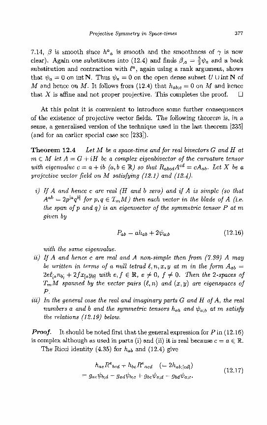
Projective Symmetry in Space-times 377
7.14, j3 is smooth since haa is smooth and the smoothness of y is now clear). Again one substitutes into (12.4) and finds /?,a = %$a and a back substitution and contraction with la, again using a rank argument, shows that $, = 0 on int N. Thus $a = 0 on the open dense subset U U int N of M and hence on M . It follows from (12.4) that habit = 0 on M and hence that X is affine and not proper projective. This completes the proof. 0
At this point it is convenient to introduce some further consequences of the existence of projective vector fields. The following theorem is, in a sense, a generalised version of the technique used in the last theorem [235] (and for an earlier special case see [233]).
Theorem 12.4 Let M be a space-time and f o r real bivectors G and H at m E M let A = G + i H be a complex ezgenbivector of the curvature tensor with eigenvalue c = a + i b (a, b E R) so that RabcdACd = CAab. Let X be a projective vector field on M satisfying (12.1) and (12.4).
i) I f A and hence c are real (H and b zero) and i f A is simple (so that Aab = 2p[aqb1 f o r p , q E T m M ) then each vector in the blade of A (ie. the span of p and q ) is an eigenvector of the symmetric tensor P at m given by
with the same eigenvalue. i i) If A and hence c are real and A non-simple then f rom (7.39) A may
be written in terms of a null tetrad l , n , x , y at m in the f o r m Aab = 2el[,nbj + 2fx[a&,] with e , f E R, e # 0 , f # 0. Then the 2-spaces of TmM spanned by the vector pairs (el n) and ( x , y) are eigenspaces o f P.
iii) I n the general case the real and imaginary parts G and H of A, the real numbers a and b and the symmetric tensors hab and $a;b at m satisfy the relations (1 2.19) below.
Proof. It should be noted first that the general expression for P i n (12.16) is complex although as used in parts (i) and (ii) it is real because c = a E R.
The Ricci identity (4.35) for h a b and (12.4) give
(12.17) h a e R e b c d + hbeReacd (= 2hab;[cdJ) = gac$b;d - gad$b;c f gbc$'a;d - gbd$a;c.
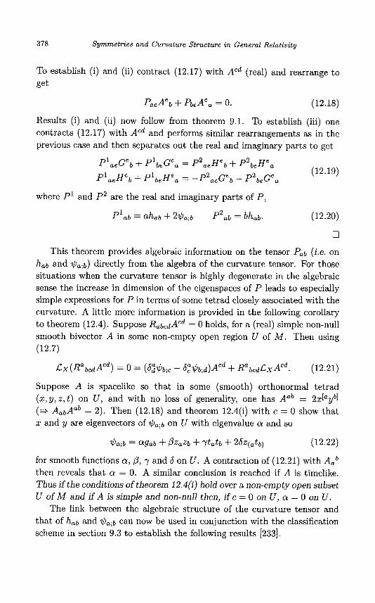
378 Symmetries and Curvature Structure in General Relativity
To establish (i) and (ii) contract (12.17) with Acd (real) and rearrange to get
P a e A e b PbeAea = 0. ( 12.18)
Results (i) and (ii) now follow from theorem 9.1. To establish (iii) one contracts (12.17) with Acd and performs similar rearrangements as in the previous case and then separates out the real and imaginary parts to get
plaeGeb + P'beGea = P2aeHeb + P2beHea P1,,Heb f PlbeHea = -P2aeGeb - p2beGea
( 1 2.19)
where Pl and P2 are the real and imaginary parts of P,
Plab = ahab + 2'l,ba;b P2,b = bhab. (12.20)
0
This theorem provides algebraic information on the tensor Pab (i.e. on h a b and directly from the algebra of the curvature tensor. For those situations when the curvature tensor is highly degenerate in the algebraic sense the increase in dimension of the eigenspaces of P leads to especially simple expressions for P in terms of some tetrad closely associated with the curvature. A little more information is provided in the following corollary to theorem (12.4) . Suppose RabcdACd = 0 holds, for a (real) simple non-null smooth bivector A in some non-empty open region U of M . Then using (12.7)
CX(RabcdACd) = 0 = (6Z$bic - 6,"'l,bb;d)ACd + RabcdCXACd. (12.21)
Suppose A is spacelike so that in some (smooth) orthonormal tetrad (2, y , z , t ) on U , and with no loss of generality, one has Aab = 2 d a y b ] (+ AabAab = 2 ) . Then (12.18) and theorem 12.4(i) with c = 0 show that x and y are eigenvectors of $a;b on U with eigenvalue Q and so
$a;b = Qgab + pzazb + " f t a t b + 26z(atb) (12.22)
for smooth functions a, p, y and 6 on U . A contraction of (12.21) with Aab then reveals that Q = 0. A similar conclusion is reached if A is timelike. Thus if the conditions of theorem 12.4(i) hold over a non-empty open subset U of M and if A is simple and non-null then, if c = 0 on U , Q = 0 on U .
The link between the algebraic structure of the curvature tensor and that of h a b and '$a$ can now be used in conjunction with the classification scheme in section 9.3 to establish the following results [233].
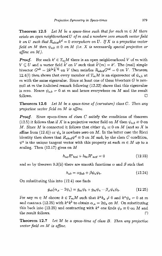
Projective Symmetry in Space-times 379
Theorem 12.5 Let M be a space-time such that for each m E M there exists an open neighbourhood U of m and a nowhere zero smooth vector field k on U such that Rabcdkd = 0 everywhere on U . If X is a projective vector field on M then '$a$ F 0 on M (i.e. X is necessarily special projective or af ine on M ) .
Proof. For each k' E TEM there is an open neighbourhood V of m with V U and a vector field k' on V such that i '(m) = k'. The (real) simple bivector Gab = 2k[ai'bl on V then satisfies RabcdGCd = 0 on V . Theorem 12.4(i) then shows that every member of TmM is an eigenvector of '$)a$ at m with the same eigenvalue. Since at least one of these bivectors G is non- null at m the italicised remark following (12.22) shows that this eigenvalue is zero. Hence = 0 at m and hence everywhere on M and the result follows. 0
Theorem 12.6 Let M be a space-time of (curvature) class C . Then any projective vector field on M is afine.
Proof. Since space-times of class C satisfy the conditions of theorem (12.5) it follows that if X is a projective vector field on M then '$a$, 0 on M . Since M is connected it follows that either 3 0 on M (and so X is affine from (12.4)) or '$a is nowhere zero on M . In the latter case the Rcci identity then shows that Rabcd@d = 0 on M and, by the class C condition, $a is the unique tangent vector with this property at each m E M up to a scaling. Then (12.17) gives on M
haeRebcd i- hbeReacd = 0 (12.23)
and so by theorem 9.3(ii) there are smooth functions a and p such that
hab = agab + P'$a'$b* (12.24)
On substituting this into (12.4) one finds
gab(a ,c - 2'$c) = gac'$b + %'$a - P,c'$a'$b. (1 2.25)
For any m E M choose k E TmM such that k"ka # 0 and ka$" = 0 at m and contract (12.25) with k"kb to obtain a," = 2qa on M . On substituting this back into (12.25) and contracting with k" one finds '$a 3 0 on M and the result follows. 0
Theorem 12.7 Let M be a space-time of class B. Then any projective vector field on M is afine.
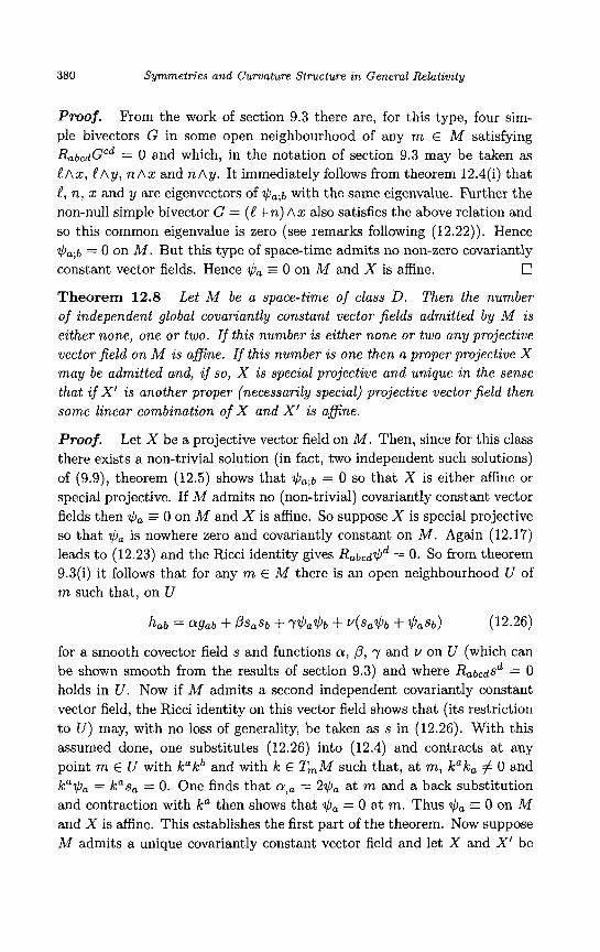
380 Symmetries and Curvature Structure in General Relativity
Proof. From the work of section 9.3 there are, for this type, four sim- ple bivectors G in some open neighbourhood of any m E M satisfying RabcdGCd = 0 and which, in the notation of section 9.3 may be taken as e A s , CAY, n A x and n A y . It immediately follows from theorem 12.4(i) that e, n, x and y are eigenvectors of $a$ with the same eigenvalue. Further the non-null simple bivector G = (C+n) A x also satisfies the above relation and so this common eigenvalue is zero (see remarks following (12.22)). Hence $ha$ = 0 on M . But this type of space-time admits no non-zero covariantly
0
Theorem 12.8 Let M be a space-time of class D . Then the number of independent global covariantly constant vector fields admitted by M is either none, one or two. If this number is either none or two any projective vector field on M is afine. If this number is one then a proper projective X may be admitted and, i f so, X is special projective and unique in the sense that i f XI is another proper (necessarily special) projective vector field then some linear combination of X and X' is afine.
Proof. Let X be a projective vector field on M . Then, since for this class there exists a non-trivial solution (in fact, two independent such solutions) of (9.9), theorem (12.5) shows that I,ba;b = 0 so that X is either affine or special projective. If M admits no (non-trivial) covariantly constant vector fields then $a = 0 on M and X is affine. So suppose X is special projective so that Qa is nowhere zero and covariantly constant on M . Again (12.17) leads to (12.23) and the Ricci identity gives Rabcd$' = 0. so from theorem 9.3(i) it follows that for any m E M there is an open neighbourhood U of m such that, on U
constant vector fields. Hence $a = 0 on M and X is affine.
hab = agab + Psasb + Y$a$b + v(sa$hb + '$'ash) (12.26)
for a smooth covector field s and functions a, P, y and v on U (which can be shown smooth from the results of section 9.3) and where Rabcdsd = 0 holds in U . Now if M admits a second independent covariantly constant vector field, the Ricci identity on this vector field shows that (its restriction to U ) may, with no loss of generality, be taken as s in (12.26). With this assumed done, one substitutes (12.26) into (12.4) and contracts at any point m E U with kakb and with k E T,M such that, a t m, kaka # 0 and ka$, = kasa = 0. One finds that a,a = 2$a at m and a back substitution and contraction with ka then shows that $, = 0 at m. Thus $a E 0 on M and X is affine. This establishes the first part of the theorem. Now suppose M admits a unique covariantly constant vector field and let X and XI be
Projective Symmetry in Space-times 381
proper (necessarily special) projective vector fields on M with associated tensors $,, h a b and I);, hbb, respectively. Then $a$ = $b;b = 0 and so, by the uniqueness assumption, $: = Ada (0 # X E R). Thus the (projective) vector field X' - AX is easily seen to be affine from (12.4) and the proof is complete. 0
In fact if M is a simply connected space-time of class D which admits a proper projective vector field then theorem 12.8 restricts the holonomy type of M to Rs, R8, R ~ o , R 1 1 and R 1 3 and it can be shown that Rs and R 8 are impossible [233].
12.3 Space-Times Admitting Projective Vector Fields
So far the theorems proved have been towards the non-existence of (proper) projective vector fields. Some cases where they do exist can now be dis- cussed [233].
In the previous theorem the situation for a space-time of class D admit- ting exactly one independent global covariantly constant vector field was not completed except to say that any proper projective vector field admit- ted was necessarily special projective and was unique up to additive affine vector fields. So let M be such a space-time with (say) a covariantly con- stant unit timelike vector field u. If X is a proper projective vector field on M then $a$ = 0 and since $a is not zero one may assume after a constant rescaling of X , if necessary, that $, = u,. Then (12.26) holds on the open subset u of M with $a = u, and s satisfying R a b c d s d = 0 on u. One can always choose s so that sass = 1 and = 0 on U and it then follows that. on U
A substitution of (12.26) into (12.4) and contractions firstly with $a$b and secondly with ljlasb yield
Again on substituting (12.26) into (12.4), contracting with $a and using (12.28) one finds
382 Symmetries and Curvature Structure in General Relativity
which, from rank considerations, shows that u is nowhere zero on U . Equa- tion (12.28) shows that v,a is nowhere zero on U.
Now for any m 6 M one may construct a local coordinate system about m by first noting that a function t exists on some open neighbourhood of m such that $a = t,a. Also, from section 4.11 example (v), the subsets of this neighbourhood of constant t and v are 2-dimensional submanifolds of M . Finally define coordinates x2 and x3 in these 2-dimensional submanifolds and let xo = t , x1 = v. In this coordinate system the metric is
ds2 = -dt2 + dv2 + g,pdx"dxP (12.30)
where a, p = 2,3. In this coordinate system one can compute Sa;b in terms of the Christoffel symbols rtc associated with (12.30) to find
(12.31) 1 1 Sa;b = sa,b - r z b s c - r a b = sgab, l
and so, using (12.29)
(12.32)
From the usual metric completeness relation this equation is identically true unless a and b take values in {2,3} and, together with the fact that the metric components are independent o f t (since u is a Killing vector field on M ) then show that gap = u2q,p where the gap are independent o f t and v (i.e. xo and x l ) and u must now be restricted by v > 0 or u < 0. Thus the metric is
v t , a t , b - u,av ,b -k gab = T g a b , l *
ds2 = -dt2 + dv2 + v2q,pdxudxP (12.33)
in some coordinate system about any point of M (2331.
fields X , Y and Z by In one of the coordinate domains described above define three vector
xa = ( t 2 , v t , 0 , 0 ) , Y" = ( t , O , O , O ) , 2" = (t,v,O,O). ( 12.34)
Then X = tZ , Y = -tu and, from (12.33) after a short calculation
(12.35)
Thus Z is proper homothetic, Y is proper affine (since Habit = 0) and X is easily checked to be proper (special) projective in this coordinate domain since hab satisfies (12.4) with $a = u,. Regarding this coordinate domain as the space-time M it follows that dim P ( M ) = dim S P ( M ) _> 4 and from
Z a ; b = gab, Y a ; b = H a b ( H a b = --'ILaUb)
( h a b = 2tgab + 2 z ( a u b ) , Fab = Z [ a U b ] . x a ; b = i h a b + F a b
Projective Symmetry in Space-tames 383
the projective, affine and homothetic "uniqueness" results (theorems 12.8, 10.2(iii) and (10.14) any further independent projective vector fields may be chosen to be Killing (since the holonomy type can not be R2, R3 or R4).
The above analysis was carried out with the assumption that the unique independent covariantly constant vector field admitted by M was timelike. If it is spacelike (and chosen to be unit and denoted by y) then one may arrange that y and s are orthogonal independent vector fields satisfying (9.9) at each m E M and again it will be assumed that $a = ya. There are now three possibilities given by the nature of the 2-spaces at m spanned by y and s. Let A, B and C be the subsets of M at each point of which this 2-space is, respectively, null, timelike and spacelike. Then M = AU B U C is a disjoint decomposition of M and locally on the closed subset A, s can be chosen null whereas locally on the open subsets B and C , s can be chosen, respectively, timelike and spacelike. Consider first the open subset int A of M where, if non-empty, one has in some coordinate neighbourhood of any m E int A
It follows that h,b may be written in the form (12.25) above. A substitution into (12.4) and a contraction with then gives the contradiction $, = 0 and so int A = 0. So A has empty interior (and if A = 0 then, since M is connected, either M = B or M = C). On the subsets B and C the analysis and results are very similar to the previous case and a proper special projective vector field is admitted.
Now suppose the unique independent covariantly constant vector field is null (and taken to be $ a ) . Then at each m E M there is s E T,M such that sa and Qa are smooth independent solutions of (9.9). Two possibilities arise given by the nature of the 2-space spanned at m by these solutions. Let A and B be the subsets of M at each point of which this 2-space is null and timelike, respectively. Then M = A U B is a disjoint decomposition of M with B open and A closed. On A, sa may be chosen spacelike and orthogonal to $a whilst on B, sa may be chosen null and satisfying = 1. So consider int A and for each m E int A choose an open neighbourhood U of m so that (12.26) holds on U . Then substitute into (12.4) and contract successively with $ a , sash and gab to obtain $, = 0 on U and so int A = (b, i.e. A has empty interior. Next for m E B choose an open neighbourhood of m on which (12.26) holds and substitute into (12.4). Successive contractions
384 Symmetries and Curvature Structure an General Relativity
with sash, gab and sa give y,a = 2sa, v , ~ = $a and
usa;b = gab - $ash - sa$b. (12.37)
(and (12.37) together with the Ricci identity confirm the relation RabcdSd = 0). So choose local coordinates xa with xo = u, x1 = w = 47, and x2 and x3 coordinates in the 2-dimensional submanifolds of constant v and y to get a metric
ds2 = 2 d ~ d w + g,gdxadxP (12.38)
where a,P = 2,3. An analysis similar to that yielding (12.33) now gives [2331
ds2 = 2d~dw + v2q,pdxadxP (12.39)
where gap is independent of u and w. For this metric define vector fields X, Y and Z by
Xa=(u2,VW,0,0) Ya=(O,v,O,O) Za=(u,W,O,O). ( 12.40)
Then Za;b = gab and so z is proper homothetic, Ya;b = $a$b and so Y is proper affine and X = vZ so X is (proper) special projective satisfying (12.1) and (12.4) with hab = 2Vgab + 2z(a$b) and projective 1-form qa. Thus regarding this coordinate domain as the space-time it follows that d imP(M) = dimSP(M) 2 4 and from the uniqueness results used pre- viously any further independent members of P ( M ) may be chosen to be Killing.
It follows from theorem 12.3 that the Schwarzschild metric admits no proper projective vector fields and, since it admits no proper affine or homo- thetic vector fields (section 10.7) the only projective vector fields admitted are just the 4-dimensional Lie algebra of Killing vector fields (10.81). Ex- actly the same is true of the Reissner-Nordstrom metric which in the usual coordinates t , r, 8,4 is given by (10.83).
To establish this, note that the absence of (proper) homothetic and affine vector fields was established in section 10.7 and so it is sufficient to show that no proper projective vector fields are admitted [236]. To see this one notes that the curvature tensor components for (10.83) can be written in the usual 6-dimensional block form (for notation see chapter 7)
Rabcd = diag(A, B , B , C, B , B) . (12.41)

Projective Symmetry in Space-times 385
The exact expressions for A, B and C , which are functions only of r , are not needed. All that is required is the knowledge that none vanishes nor are any two of them equal over any non-empty open subset of the space- time manifold M . Thus the curvature tensor has four independent real eigenbivectors el A e2, e1 A e3, e2 A e0 and e3 A eo with real eigenvalue B ( p ) at any p E M where eO, e l , e2 and e3 are, respectively, mutually orthogonal unit vectors at p in the directions of 6, &, and q. Also e2Ae3 and e'Aeo are real eigenbivectors with real eigenvalues A ( p ) and C(p) , respectively, at p. Now let X be a projective vector field on M so that (12.1) and (12.4) hold for X" and its corresponding tensors h a b and qa. Then theorem (12.4)(i) shows that eO, e l , e2 and e3 are everywhere eigenvectors of the symmetric tensor Bhab+2$,;b with equal (real) eigenvalues and thus
Bhab + 2$'a;b = Pgab (12.42)
for some function P on M . Similarly e2 and e3 are eigenvectors of Ahab + 2'$a;b with the same real eigenvalue, and similarly for eO, el and Chab+2Ga;b. Thus, on M (see section 7.5)
a a
Ahab f 2$a;b = Y a b + p(e2,e2b -t e3 ae b ) (12.43)
Chab + 2$a;b = Z a b + V(e',e'b - eoaeob) ( 12.44)
where Y a b and Z a b are, respectively, collections of symmetrised products of eoa and ela and of e2a and e3a and p and v are functions on M and whose precise forms are not required. Since A, B and C are distinct over an open dense subset U of M , subtractions of (12.42) from each of (12.43) and (12.44) lead to the facts that over U e0 and e1 are eigenvectors of hab with equal eigenvalue and similarly for e2 and e3. Hence there exists functions p and cr on U satisfymg
1 1 0 0 hab = p(e ae b - e ae b ) + ff(e2,e2b + e3,e3b) (12.45)
where the completeness relation gab = qcdecaedb has been used. Now sub- stitute the second relation in (12.45) into (12.4) and contract successively with gaib and eaeb to get (recalling that eaea = 0 + ea;bea + eaea;b = 0 , etc.) Gaga = = = = 0 and hence that = 0 on U and hence on M . Then (12.4) reveals that X is &ne (and so not proper projec- tive) on M . This completes the proof. A similar argument to the above but
= ffgab + ( p - ~ ) ( e l a e l b - eoaeob>
2 3 0 1 0 1 0 1
386 Symmetries and Curvature Structure in General Relativity
with A = C on M reveals the result (again) for the Schwarzschild metric. In fact for each of these metrics X must be Killing.
An argument using similar techniques can be used to show that null Einstein-Maxwell fields can never admit a proper projective vector field [237]. In this case the argument is more complicated because of the need to decompose the space-time into Petrov types.
For the FRW (conformally flat perfect fluid) models the above tech- niques enable the problem of the admission of projective vector fields to be approached in a similar manner 12381. Here, a very brief sketch of the argument will be given. The metric g in the usual coordinates is given by (10.84) where t (= zo) is the cosmological time coordinate and R(t) a function o f t controlled by the Einstein field equations for a perfect fluid. The metric g induces a positive definite metric of constant curvature in the hypersurfaces of constant t . This constant curvature is represented in a conventional way by a parameter k which is zero when these hypersurfaces are flat and f l otherwise (for details see e.g. [239]). The (timelike fluid) flow vector on this space-time M is u = & with components in the above coordinates given by ua = baO, u, = -boa = -t,a and which satisfies
(12.46)
where the expansion 0 3 ua;, of u is a function only of t and is related to R by 3R = Re (and . = s).
Two special cases of these models can be quickly considered. They are, firstly, the case when the space-time metric (10.84) is actually of constant curvature (the de-Sitter type metrics) and in these cases the situation is known [234]. The second case is the Einstein static type (8.14) which can, essentially, be realised by (10.84) with u covariantly constant, Ua;b = 0 (and hence, from (12.46), 0 = 0 and R = constant). The curvature tensor for the general metric (10.84) takes the (6 x 6) form
e Ua;b = ?(gab + U a u b )
where fl and f2 are functions only of t . Since M is assumed (as always) non-flat (so that the curvature tensor never vanishes over a non-empty open subset of M ) it follows that the curvature rank is at least three over an open dense subset U of M . In the Einstein static case, Ua;b = 0 * Rabcdud = 0 and so the rank on U is three. Then theorem 12.6 confirms that no proper projective vector fields exist.
Projective Symmetry in Space-times 387
The case considered next is the “general” local situation with M = I x H with I some open interval of R (playing the role of an interval of time t) and H a 3-dimensional connected manifold of constant curvature (a connected open subset of the hypersurfaces of constant t). It will be assumed that no non-empty open subset of M is of the de-Sitter or Einstein static type and so the functions fl and fi in (12.47) are distinct on some open dense subset of M . Also M is assumed to admit a 6-dimensional Killing algebra K ( M ) with 3-dimensional spacelike orbits of constant t each isometric to H . Then any X E K ( M ) induces a Killing vector field X in an orbit t = t o with respect to the induced metric of that orbit (theorem lO.ll(ii)) and the map x . X --f X is a linear map between the Lie algebras K ( M ) and K ( H ) . It is also one-to-one, from theorem lO.ll(iii), and onto (since dim H = 3 + dimK(H) 5 6). Hence x is a Lie algebra isomorphism (and so dimK(H) = 6). Thus every Killing vector field in a hypersurface of constant t (with induced metric) can be regarded as arising naturally from a unique space-time Killing vector field.
Another feature of the hypersurface geometry of H which is important in this context is its homothetic symmetry. Suppose there exists a proper (local or global) homothetic vector field in the induced geometry in H . Then, since H has a transitive Killing algebra, it follows that for any p E H there is such a proper homothetic vector field Y defined in some neighbour- hood U of p in H . Then either Y(p) = 0 or else Y(p) # 0 and there is a Killing vector field on H such that X ( p ) = Y(p) . Then 2 = X - Y ($0) is proper homothetic on U and Z ( p ) = 0. So for any p E H some (local or global) proper homothetic vector field on H vanishes at p . Then theorem 10.5(iii) modified so as to apply to the 3-dimensional positive definite case shows that all Ricci eigenvalues and hence the Ricci and Riemann tensors in the geometry of H vanish at each p E H. Thus H is flat. It follows that in the cases of FRW models with k = f l can there be no (hypersurface geometry) proper homothetic vector fields in H . They exist, of course, if H is flat (k = 0).
The proof now proceeds (briefly) in the following steps. First let X be a projective vector field on M . Then (12.47) and theorem (12.4)(i) show that
hab = ffuaub + Pgab (12.48)
for functions a and P. Then use of (12.4) and (12.46) and certain contrac- tions shows that a and ,6 are functions only of t , that a+,B is constant, that +a = Xua with X a function only o f t and that 3X = a0 and a,, = -2Xua.
388 Symmetries and Curvature Structure in General Relativity
Next write X as X" = yu" + q" where the vector field q on M satis- fies qaUa = 0 and y is a function on M . The expression (7.7) solved for the Ricci tensor in terms of the fluid pressure and density (which depend only on t ) and (12.7) can be used to show that y is a function only of t. Now suppose y vanishes over some non-empty open subset of M . Then it vanishes everywhere in the open subset U = (to,tl) x H of M , for some to, t l E E% with to < t l , and so Xaua = 0 on U. Thus Xa;bUaUb = 0 and hence h,buaub = 0 on U. This leads (recalling the exclusion clauses on M ) to X being Killing on M . So if non-Killing members of P ( M ) are being sought, one assumes X is not Killing and hence that y does not vanish on any non-empty open subset of M . The expression Xa = yua + qa is then substituted into (12.1) to show that q defines in a natural way an (induced geometry) homothetic vector field in the hypersurfaces of constant t (i.e. in H ) . In the cases k = f l no proper such homothetic vector fields (as shown earlier) and this leads to the fact that q is a Killing vector field on M and that X" - qa = yu". Thus, up to Killing vector fields, one need only study projective vector fields of the form Xa = y(t)ua in the cases k = f l (and for such vector fields the projective bivector F in (12.1) can then be checked to be identically zero. Equations (12.1) and (12.4) then lead to differential equations relating a, y and 9 from which it can be concluded that the FRW metric (k = fl) does not, in general, admit proper pro- jective vector fields but does so for certain special choices of the function R(t). A similar conclusion can be achieved in the k = 0 case, but care is needed here since H now admits (local or global) proper homothetic vector fields. Full details are available in [238]. A by-product of this calculation is the finding of those FRW models which admit proper homothetic vector fields, a result which was already known (section 10.7). The FRW models are examples of conformally flat perfect fluid space-times. In fact theorem 12.4 may be used to show that the only conformally Aat perfect Auid space times which admit proper projective vector fields axe the special cases of the FRW models alluded to above [240]. In this reference the fact that the assumptions made implied the existence of an equation of state between the pressure and density of the model was omitted. A proof of this fact can be found in [241].
Projective Symmetry in Space-times 389
12.4 Special Projective Vector Fields
Special projective vector fields were encountered in section 12.3 and also for Minkowski space in (12.9). In this section the general situation when a special projective vector field exists will be described. The ideas and results are very similar to those discussed for special conformal vector fields in section 11.7 and so only a summary will be given (for details see [233],[232]).
Suppose M is non-flat and admits a proper special projective vector field X satisfying (12.1) with projective 1-form $a satisfying $a$ = 0. Thus $a
is nowhere zero and $a$a is constant on M . So suppose $a$a # 0 (so that $a is non-null on M) . Using the projective bivector F define a global vector field Y on M in components by Ya = F b a $ b and use (12.5) to get
Thus from (10.8) and (10.10) Y is proper affine and is everywhere orthog- onal to $". Just as in the conformal case Ya and $a have vanishing Lie bracket and give rise to a 2-dimensional integrable distribution over an open dense subset of M . It follows that Rabcd$d = RabcdYd = 0 and the geome- try of the integral manifolds of this distribution is as in the special conformal case. In particular, the curvature rank is one over an open dense subset U of M where, it may be assumed without loss of generality, Y is non-zero and together with $" gives rise to the above mentioned distribution. It now follows from theorem 12.8 that M admits a unique (up to a constant scaling) covariantly constant vector field and that if X , X' E S P ( M ) then some linear combination of them is affine and so dim SP(A4) (= dim P ( M ) from theorem 12.8) = dimA(M)+l (= d imH(M)f2 from theorem 10.14).
Now assume M is simply connected (or restrict to a simply connected region) so that one may write $a = $,a for some function $. Then construct vector fields P and Q where
= -~($J~$J~)- ' (Y" - ;$$") Pa = $&". (12.50)
Then from (12.49) one finds
where

390 Symmetries and Curvature Structure in General Relativity
Thus P is (proper) special projective, with the same projective l-form as X and is tangent t o the integral manifolds described above. Also Q is proper homot hetic.
Now it is recalled that in Minkowski space-time a basis for P ( M ) could be chosen for which only 4 of the 24 members were proper projective and, in fact, special projective (from (12.9)). A choice of these vector fields can be made by choosing, successively, 8" = S:, . . . , d i and then each equals some function f multiplied by the homothetic vector field on Minkowski space with components ( t , x , y, z ) and where f," = 8, is the associated projective l-form. For example, the choice Oa = d: gives, in (12.9), X" = t ( t , x , y,z) and f = t so that f , a = 8,. Then X a = t(-t, x , y, z ) and h a b = 2x(a,b) is easily shown to satisfy (12.4) with 11," = Ba. That such a choice is available generally follows from (12.50)-(12.52).
The similarity between the studies of the Lie algebras S C ( M ) and S P ( M ) can be taken further. First assume M simply connected (or work on a simply connected coordinate domain of M ) . If M admits a proper member X of S P ( M ) with projective l-form $a non-null (so that 0 # = constant), there is an associated homothetic vector field Q as in (12.50). Now Qa and 11," are each local gradients and so (by sim- ply connectedness) they are each global gradients 11," = Qa = a,, for functions +,a : M + R. The global vector field E" = $Q" - a$" then satisfies E a ; b = $gab + 2Q[a$b~ and so is special (proper) conformal (with 11, playing the role of 4 in (11.1)). Conversely, let M admit a (proper) spe- cial conformal vector field X satisfying (11.1) with 0 # q5"q5" = constant. Then define the global vector field E'" = (&Y)-lq5Wa with W given as in (11.47). Then if Hab = 2E[a;b) it follows that Hab satisfies (12.4) with 11," replaced by 4". Hence E' is special (proper) projective. It is noted that this converse proof did not require the simply connected assumption. The following theorem is thus established.
Theorem 12.9 The set of simply connected space-times which admit a special (proper) conformal vector field satisfying (1 1.1) with # 0 and those which admit a special (proper) projective vector field satisfying (12.1) and (12.4) with I)"$" # 0 are, in the sense described above, identical.
If (only) the simply connectedness assumption is dropped it is still true that those space-times which admit a proper member of S C ( M ) also admit a proper member of S P ( M ) but now those space-times which admit a proper member of SP( M ) have only been proved to admit a proper member of S C ( M ) locally (i.e. in some open neighbourhood of any point of M ) . It
Projective Symmetry in Space-times 39 1
is also noted that the theorem is false if the conditions # 0 # $a$a
are dropped. To see this note that the vacuum plane wave space-times can admit proper members of SC(M) (section 11.5) with null but can not admit any proper projective vector field from theorem 12.3. Something, however, remains of these results in the case $a$a = 0. Suppose M admits a proper special projective vector field X with projective 1-form $, satisfying $a;(, = 0 and $"$, = 0. Then (12.39) gives a local form for the metric and reveals an expression (12.40) for X in a coordinate domain U as X = uZ where is homothetic and Za;b = gab. so again X can be chosen as u times a proper homothetic vector field, where $, = u,,. Further, from (12.40) one can write Z, = Z,, where Z = uw. Then the vector field XIa = uZ" - Z$" (= u2sa) satisfies X& = Ugab + 2Z[,$b] on U and is hence (proper and) special conformal on U with conformal function u.
One can add a little more here to the uniqueness result established for SP(M) in this section. Suppose M admits a proper member of SP(M) whose projective 1-form satisfies +a+a # 0. Then the previous work shows that the curvature rank on M is at most one and so if X is any mem- ber of P(M) it must be special by theorem 12.5. Hence in this case P(M) = SP(M). Also, if M is simply connected and admits a proper member of SP(M) with $a+a # 0, then since M admits covariantly constant, proper homothetic and proper af€ine vector fields, the unique- ness results so far given show that dimP(M) = dimSP(M) > 4 and dimSP(M) = dimA(M) + 1 = dimK(M) + 3. The same argument as in section 11.7 shows that dimK(M) 5 4 and so 4 5 dimSP(M) (= dimP(M)) 5 7. If M is not simply connected this becomes a local result.
12.5 Projective Symmetry and Holonomy
Theorems 12.4-12.8 suggest a connection between the existence of projective vector fields and the curvature rank and hence the holonomy type of M . This will be explored further in this section. First it is convenient to return to the curvature tensor classification described in section 9.3 and to the (disjoint) decomposition of M into the subsets A, B , C, D and 0. In that section it was stated that M could be disjointly decomposed as
M = A u int B u int C u int D Uint 0 u Z (12.53)
392 Symmetries and Curvature Structure in General Relativity
where A is open and Z is closed with int Z = 0. This result will now be briefly established. To do this, some remarks on the range space B, of the linear map f in section 9.3 will be useful.
(i) If m E A U B there does not exist Ic E T,M, k # 0, such that
(ii) If m E A, dim B, 2 2 and if dim B, 2 4 then necessarily m E A. (iii) If all members of B, are simple, dimB, 5 3 and if, in addition,
dim B, = 2, there exists k E T,M, k # 0, such that Fabkb = 0 for all F E B,.
Fabkb = 0 for all F E B,.
Remarks (i) and (ii) follow from the definitions of the curvature classes. For (iii) if dim B, = 2 and all members of B, are simple then let { F, G} be a basis for B, with F, G simple and F+XG simple for each X E R. Applying condition (v) of theorem 7.1 to these bivectors gives Fab*Gbc+Gab*Fbc = 0. Then there exists k' E T,M, k' # 0 , such that Fabklb = 0 and one contracts the previous equation with k: to obtain (khG"b)*F,b = 0. Thus either the vector Gabklb is zero or it is in the blade of G and orthogonal to the blade of * F (and hence in the blade of F ) . In either case the blades of F and G intersect non-trivially and the vector k claimed in (iii) exists. Now suppose all members of B, are simple and dim B, 2 4. With F and G as above and with H E B, such that F , G and H are independent, one may use the previous argument to show that there exist p , q, r, s E T,M such that F = p A q, G = p A r and either H = q A r or H = p A s. Now repeat the argument with a fourth independent K E B,. It is easily checked now that one either contradicts the independence of F , G , H and K or the original assumption that all members of B, are simple.
Now define the subspace Urn E T,M associated with B, to be the span of the union of the blades of members of B, (including each of the canonical pair of blades for non-simple members of B, - see section 7.2). Then if m E D , dimB, = 1 and dimU, = 2, if m E C, dimB, = 2 or 3 and dimU, = 3, if m E B, dimB, = 2 and dimU, = 4 and if m E A, dimB, 2 2 and dimU, = 4. It is also useful to note that if F E B,, so that for some bivector F' at m, f(F') = F , there exists a smooth bivector F on some open neighbourhood W of m such that F(m) = F' and hence a smooth bivector RabcdFcd on W which is in B,) for each m' E W and which equals F at m. From this it is easy to check that if k E Urn then (reducing W if necessary) there exists a smooth vector field k on W such that k(m') E Urn, for each m' E W and k(m) = k . It follows (section 3.11) that there exists an open neighbourhood W' of m such that
Projective Symmetry in Space-times 393
dim Umt L dim Urn for each m‘ E W’. Clearly, W’ may be chosen so that one also has dim B,, 2 dim B, for each m’ E W’.
To establish the decomposition (12.53) let m E A so that dim B, 2 2 and dimU, = 4. Then the above argument reveals the existence of an open neighbourhood N1 of m such that dim Urn! = 4 for each m‘ E Nl and so iV1 5 A U B. If dim B, 2 3 one may take N I C A. If dim B, = 2, B, must contain a non-simple member and hence two independent non-simple members whose canonical blade pairs do not coincide and so by continuity there is an open neighbourhood N2 of m such that N2 n B = 0. Hence N1 n Nz & A. This argument shows that A is open. Now let m E B so that Bm contains a non-simple member. Continuity then shows that B,I contains a non-simple member for m’ in some open neighbourhood N3 of m and so N3 C A U B. Thus A U B is open. A simple curvature rank consideration then shows that AUBUC and AUBUCUD are open. Finally, to show int 2 = 0 let W C Z be open. Then by disjointness W n A = 0. Also, since A U B is open, W n B = W n ( A U B ) is open and since 2 is disjoint from int B, W n B = 0. Similarly, W n C = W n D = W n 0 = 0 and so W = 0. It follows that int 2 = 0.
Before the final theorem is given it is instructive to recall equations (12.17) and (12.18) in the proof of theorem 12.4 for the case where AQb is a real eigenbivector of the curvature tensor with zero eigenvalue (c = 0). The interplay between these equations is essentially that if “sufficient” solutions for Aab of (12.18) exist then $ ~ ~ ; b c( gab. But this last condition is equivalent to the vanishing of the right hand side of (12.17) and hence the left hand side. This latter condition then heavily restricts h according to theorem 9.3. This link was used in [233] to rule out proper projective vector fields in space-times of certain holonomy types but where dim B, was assumed constant. With the help of the decomposition (12.53) this theorem can now be established without this restriction [242].
Theorem 12.10 Let M be a non-flat simply connected space time.
a) If M has holonomy type R2, R3, Rq, Rs) R7, Rg or R12 then M does not admit a proper member of P ( M ) .
ii) If M admits a proper member X of P ( M ) then it has holonomy type R ~ o , R11 or R13 if and only if X E S P ( M ) . If these equivalent condi- tions hold then some open dense subset of M is of class D .
Proof. For (i) let X be a projective vector field on M and let M be decomposed as in (12.53). The members of this decomposition will be con-
394 Symmetries and Curvature Structure in General Relativity
sidered separately in the case that they are not empty. It is then clear from theorems 12.6 and 12.7 that the projective 1-form 11, vanishes on int B and int C. Next, the assumption regarding the possible holonomy types of M and the fact that, loosely speaking, B, is at each m E M contained in the infinitesimal holonomy algebra and hence the holonomy algebra enables sufficiently many solutions G of RabcdGCd = 0 to be calculated for theorem 12.4 to be invoked at each m E A and to check that, on A, $a;b = Tgab
for a smooth function y : A -+ R. Then from (12.17) and theorem 9.3 it follows that hab = &ab for a smooth function p : A + R. Thus (see the penultimate paragraph of this chapter) $ = 0 on A. If m E in tD and $(m) # 0 then $ is non-zero over some open connected and simply con- nected neighbourhood U of m and theorem 12.8 and the remark following its proof show that the holonomy type of U is either Rlo, R11 or R13. These subalgebras can not be contained in those of the stated holonomy types of M and so $ = 0 on int D. Since M is non-flat, int 0 = 8 and so 1c, vanishes on the open dense subset M \ Z of M and hence on M and X is not proper.
For (ii) let X E P ( M ) be proper and let M have holonomy type Rlo, R11 or R13. Then the appropriate definitions show that A and B are empty sets in (12.53) and so M = C u int D U Z with C open by the rank theorem. It now follows from theorem 12.6 that .1c, = 0 on C and from theorem 12.5 that $a$ = 0 on int D. Thus $a$ = 0 on M \ Z and hence on M and so X E S P ( M ) . One can also conclude because of this that, since X is proper,
cannot vanish anywhere on M and so C = 8 and M = D U Z with D open and dense in M . Conversely, if X is a proper member of S P ( M ) , it follows from section 12.4 that M = D U Z in (12.53) and from theorem 12.8 that $ is the unique independent global covariantly constant (co)vector field on M . When this restriction on the holonomy type is combined with part (i) of the theorem only the holonomy types Rlo, R11 or R13 remain0
If the conditions and conclusions of part (ii) of this theorem hold then the metric is of the form (12.33) in the R13 case (or its equivalent for spacelike $ in the Rlo case) or (12.39) in the R11 case in some coordinate domain of any point of the open dense subset D of M . It is also remarked that if a non-flat simply connected space-time M admits a proper projective and a proper f i n e vector field it must have one of the holonomy types R ~ o , R11 or R13 as described above. This follows from part (i) of the above theorem and theorem 10.14.
Theorem 12.10 is essentially a complete description of projective sym- metry for all holonomy types except Rg, R14 and R15. Part (i) of this
Projective Symmetry in Space-times 395
theorem can also be established by a direct curvature rank decomposition of M but the curvature class decomposition (12.53) leads to a more elegant proof. Some limited information on the holonomy types Rg, R14 and R15 is available [233],[242] (including a “local uniqueness” result in the Rg and R14 types) and the F.R.W. metric example in section 12.3 is of holonomy type Rl5. For examples in space-times of holonomy types Rg and R14 con- sider the metric on a global chart u, v, x, y, restricted only by u,v > 0, and given by [242]
ds2 = 2dudv + + v2ef(z’y) (dx2 + dy2) (12.54)
for some smooth function f on R2. It can then be checked that the vector field with components (1, O , O , 0) is null and recurrent on M and, from a calculation of the curvature tensor and use of theorems 8.7 and S.S(iiil.
\ , I
a2.f a2.f that the holonomy type of (12.54) is Rg if - + - = 0 on M and R14
ax2 au2 - Y
otherwise. Then the vector field X with components (uv,v2,0,0) can be shown to be proper projective on M with projective l-form Qa = (0, 1,0, 0).
So far, one has for the various symmetry algebras of M the inclusions K ( M ) C H ( M ) C A ( M ) C P ( M ) and H ( M ) C C ( M ) . It can, in fact, be established that the fork on these inclusions really does occur at H ( M ) in the sense that a vector field X on a simply connected space-time M is simultaneously in P ( M ) and C ( M ) if and only if X E H ( M ) . To see this, briefly, let x E P ( M ) f l C ( M ) . Then from (12.1) and (11.1), hab = Xgab satisfies (12.4) for some function x and l-form Qa. A substitution into (12.4) and the usual contractions then shows that Qa = 0 and x , ~ = 0 and hence that X E H ( M ) . The converse is clear.
An alternative approach to projective symmetry has been given using an algebraic study of the tensor h in (12.1). Further details of this can be found, for example, in [63],[243].

This page intentionally left blank
Chapter 13
Curvature Collineations
13.1 Introduction
The symmetries discussed so far have a number of general properties. They were represented by finite-dimensional Lie algebras and hence had a well- behaved orbit structure and each vector field in the algebra was uniquely determined by its value and those of finitely many derivatives at some point of the space-time M and possessed nice differentiability properties. Unfortunately not all symmetries of the important geometrical objects of space-time have such pleasant properties and this chapter will, by consider- ing symmetries of the curvature tensor, attempt to draw attention to some of these problems [244], [245] , 12461.
13.2 Curvature Collineations
Let M be a (smooth) space-time with (smooth) Lorentz metric g and asso- ciated curvature tensor R. Let X be a global vector field on M assumed for the time being to be C1. If the C1 local diffeomorphisms (section 5.11) as- sociated with X are denoted by & then X is called a curvature collineation if either and hence both of the following two equivalent (section 5.13) con- ditions hold [244]
- (i) C x R = 0 (i.e. LxRabcd = 0)
(ii) q5rR = R for any $t associated with X (13.1)
One problem concerning such a vector field X lies in the degree of differentiability assumed for X . Clearly one requires a t least C1 for (13.1) to make sense. So let 4t be a local diffeomorphism associated with X with
397
398 Symmetries and Curvature Structure in General Relativity
(open coordinate) domain U and (open) range W E c$~(V) as in section 10.1 with coordinates xa on U and the functions ya = xa o 4;' on W . If q5t is smooth then W and ya constitute a coordinate neighbourhood of M (since M is smooth) on which the curvature R on M and the tensor &'*fi coincide according to (13.1). These coincident tensors on W are then, respectively, the curvature tensors of the (smooth) metrics g and q5t1*g on W . If, on the other hand, 4t is Ck (1 5 k < 00) then W and ya do not constitute a chart of M (since M is smooth). However C$;'*R is still smooth with respect to M (since it coincides with A) and could be regarded as the curvature tensor of the metric 4 t ' * g on W if this metric were C2. This will be achieved if X and c $ ~ are C3. If, however, curvature collineations which are not smooth are admitted then the set of all curvature collineations, whilst clearly a vector space, is not a Lie algebra since if X and Y are curvature collineations, [ X , Y] may not be differentiable.
In spite of the fact that curvature collineations that are not smooth may (and, as will be seen later, do) exist, little is lost in the general discussion in assuming them smooth. In what is to follow, it will be indicated where and how non-smooth ones exist. So a curvature collineation is taken as a smooth global vector field X on M satisfying (13.1) and the set of all such curvature collineations is, from a result in section 5.13, a Lie algebra denoted by CC( M ) .
Further problems arise with curvature collineations when compared with the symmetries so far studied. For example, the &ne (including Killing and homothetic), conformal and projective algebras are all finite-dimensional and their individual members are uniquely determined by specifying their values and those of finitely many derivatives at some point of M (and are identically zero on M if they vanish over some non-empty open subset of M ) . It will be seen in later examples that none of these results need hold for (smooth) curvature collineations.
The following theorem is immediate from theorem 11.11 and from (12.7).
Theorem 13.1 Let M be a space-time.
i) A n y a f i n e vector field i s a curvature collineation.
ii) A conformal (respectively projective) vector field i s a curvature collineation if and only if it i s special conformal (respectively special projective).
Thus in the notation so far established, K ( M ) , H ( M ) and A ( M ) are
Curvature Collineations
subalgebras of CC(M) and
399
C ( M ) n C C ( M ) = S C ( M ) , P ( M ) n CC(M) = S P ( M ) (13.2)
A curvature collineation is called proper if it is not affine. There is a convenient way of obtaining quite general information on
the existence of curvature collineations. Let X E CC(M) and let the lo- cal diffeomorphisms associated with X be represented by the maps $t. As in section 10.1 let cPt be a particular such map with domain U and range W = $t (U) . Now, as earlier, consider the tensor pullback map $t'* which transfers tensors on U to tensors on W . If g and R are the (restricted) metric and associated curvature tensor on U from M , then &'*g is a met- ric on W with associated curvature tensor $t'*R. Since X is a curvature collineation $t'*R and R are equal and have g and &'*g as associated metrics. It follows that, on W , g and $ t l*g are related, pointwise, accord- ing to theorem 9.3. Thus using theorem 9.4 one sees that if the curvature tensor of M is of class A at each point of M (and this is automatic if the curvature rank is at least four at each point of M ) then g and $ t ' * g are conformally related with a constant conformal factor. So one has the following general result regarding curvature collineations [I191 [247].
Theorem 13.2 curvature collineation on M is a homothetic vector field.
Let M be a space-time of curvature class A. Then every
Furthermore, for a fked space-time manifold M and considering the set of all smooth Lorentz metrics on M , it is generic for the metric (i.e. the space-time) considered to satisfy the condition that the curvature rank is everywhere at least four (theorem 7.17 (iii)). Hence generically (on space- times) every curvature collineation is homothetic.
It is remarked that an alternative proof of (part of) this theorem can be obtained by taking the Lie derivative of (9.6) and using (13.1) and theorem 9.4 [247], [244].
For a vacuum space-time which has constant curvature class this class must be A or C (and the latter case corresponds to Petrov type N since now the curvature and Weyl tensors are equal - see the proof of theorem 9.6). Thus the following theorem now follows from the previous one.
Theorem 13.3 If M is a vacuum space-time with constant curvature class then either A4 is of Petrov type N or every curvature collineation on M is a homothetic vector field.
400 Symmetries and Curvature Structure in General Relativity
13.3 Some Techniques for Curvature Collineations
One way of studying curvature collineations is suggested by section 9.3. One could consider examples of space-times of class B , C or D (in the notation of that section). It then follows from that section, the earlier discussion of this chapter and the definition of the Lie derivative in section 5.13 that if X E C C ( M ) the local expressions for C x g are, from (9.10)-(9.12) for the above spacetime classes B, C and D, respectively,
CXgab = 4gab 2Xl(anb) = (4 f X)gab - X(xaZb + Y a Y b )
CXgab = dgab f Xwawb (13.3)
CXgab = $gab + puaub + 2vu(aVb) + Xuaub
for smooth functions 4, p, v, X (the smoothness following from the theory in section 9.3). This will now be applied to special types of spacetimes of classes C and D and essentially in full generality for class B.
First let M be a simply connected space-time (or open region of space- time) of class C and of holonomy type R13. Then M admits a global, smooth, covariantly constant unit timelike vector field u. The associated covector field ii (with local components ua) is a global closed 1-form and hence is exact since M is simply connected (section 4.16). Thus there exists a global smooth function f : M -+ R such that ii = d f . For such spacetimes one can choose about any point a natural product coordinate domain U with coordinates xa and then the hypersurfaces of constant xo in U coincide with the intersection of the hypersurfaces of constant f with U . Also one can arrange that, in U , ua = 6; (3 ua = -6:) and the metric is (section 8.3)
(13.4)
where the gao depends only on xa (a, p, y = 1,2,3) . The Ricci identity shows that in any coordinate system in M , Rabcdud = 0 and so k = u is, at each point of M , the unique independent solution of (9.9). In the special coordinates on U the components Rabcd and R a b c d (and also are zero if any of the indices a, b, c or d equals zero and the components gag are the induced metric components in the hypersurfaces of constant xo in U (in the coordinates xa). Any two of these hypersurfaces are isometric under the map given in an obvious notation by (xa, x o ) -+ (xa, xo + to ) for appropriate to E R.
Now consider the existence of a global curvature collineation X on M .
Curvature Collanentaons 401
The discussion will be given globally by a component argument in any coordinate system in M (but sometimes the special coordinate system in U is useful). Thus (13.1) holds and so in any coordinate system on M , using the second of (13.3), dropping a factor 4 and relabelling
Xa;b = 4 g a b + A u a u b + Fab (13.5)
for smooth functions 4 and X and smooth bivector F on M . Then (13.1) gives
Rabcd;eXe + RaecdXe;b + RabedXe;c + RabceXe;d - RebcdXa;e = 0. (13.6)
A contraction of this result with u, reveals
Rebcd(Xa;,Ua) = 0. (13.7)
So by the uniqueness of solutions to (9.9) one sees that X a i e u , is pro- portional to u, and then (13.5) shows that F,bub 0: u, and hence that F,bub = 0. One can now make a global decomposition of X on M accord- ing to
x = x’ - au a = xau, (13.8)
where a is a global smooth function and X’ a global smooth vector field on M . Clearly X’ is everywhere orthogonal to u, Xlau, = 0 , and is hence tangent to the submanifolds of constant f (and to those of constant zo within U ) . Then a contraction of (13.5) with ua shows, since F,bub = 0, that a,, = (4 - A)u, (or da = (4 - X)df) and so in the coordinate system in U , a and (4 - A) are functions of zo only. Now since u is covariantly constant it is necessarily a curvature collineation and so X = u satisfies (13.6). Substituting into (13.6) gives R a b c d i e u e = 0 and it is then a straightforward matter to see from (13.6) that au and hence (from (13.8)) X’ are curvature collineations on M . Furthermore, (13.5) and (13.8) easily reveal that [X’ ,u] = 0. This is equivalent to LUX’ = 0 and has the geometrical interpretation that if Xt represent the local isometries between the xo =constant hypersurfaces in U arising from the vector field on U then X‘ (on U ) is “invariant” under Xt* (i.e.Xt*X’ = X’) and the vector fields in each hypersurface of constant xo in U naturally induced by X‘ are mapped to each other by the restrictions of Xt* to these hypersurfaces. Put more simply, in these coordinates XIo = 0 and the XIa are independent of zo. Each of these (isometric) hypersurfaces in U has a metric g a p and curvature tensor Rap+ (and the Christoffel symbols I?& where I?tc are the
402 Symmetries and Curvature Structure in General Relativity
Christoffel symbols on U ) . It is then easily checked from (13.6) by setting a, b, c and d equal to Greek indices a, p, y and b and noting that one can change the semi-colon derivative to a covariant derivative with respect to the hypersurface geometry (because of the properties of rEc mentioned earlier) that the vector field 2' with components 2Ia = XI" induced in these hypersurfaces from X' is a curvature collineation in the hypersurface geometry. But (13.5) reveals more. It projects onto each hypersurface in the form (using a stroke for a hypersurface covariant derivative)
*hip = &lap + Fap (13.9)
which can be calculated directly from (13.5) (In fact, if one uses (5.15) with 4, X, Y and T replaced, respectively, by a , 2, X and g where i is the inclusion map from the hypersurface to M and h = i*g is the hypersurface metric one gets from (13.5) C 2 h = 24h which is the symmetric part of (13.9)). Since one can construct a coordinate domain like U about any point of M it follows that the vector field induced in the hypersurfaces of constant f by X' is a conformal vector field in the induced geometry. Now if one takes the covariant derivative of (13.5), uses the Ricci identity on X, contracts with uc and takes the symmetric part on the indices a and b one finds using F a b u b = 0 and after a simple rank argument that &ua = 0 and so in the coordinates on U , 4 is independent of xo. Further, from the class C condition, the hypersurface curvature components Rapr& in the coordinates xa in U have rank two or three at each point of M . The obvious adaptation of the work in section 9.3 applied in three dimensions shows that the curvature tensor Rapr& determines its metric up to a constant conformal factor and so the vector field X' induced in the hypersurfaces of constant f which is already known to be a curvature collineation in the induced geometry is homothetic in the induced geometry. Thus 4 is a constant on M . Since it was shown earlier that ( 4 - A) was, in each coordinate domain U , a function of xo only, it follows that X also depends only on xo in each such domain and so X depends only on f . One final point to note is that it is easily checked that u, fu, . . . , f"u are curvature collineations on M by direct substitution into (13.6). But since ii = df, f is not constant on M and so they are independent members of C C ( M ) for each n. Hence the Lie algebra CC(M) is infinite-dimensional and each member can be decomposed as in (13.8). Similarly, restricting attention to U , one gets the Lie algebra of curvature collineations CC(U) on U and each member of CC(U) can be decomposed uniquely as in (13.8). Thus CC(U) is the vector

Curvature Collineations 403
space direct sum of the vector space of all vector fields of the form g(xo)u for some arbitrary smooth function g (each of which is easily checked to be in CC(U) - cf. [244]) and the finite-dimensional vector space of homothetic vector fields of each (any) hypersurface in U of constant zo together with its induced geometry. It is remarked that it is easily checked that the sum of such a homothetic vector field and a vector field of the form g(zo)u is in
It should be clear from the arbitrary functions involved in describing CC(M) how one might choose X E C C ( M ) which is not C", or not uniquely determined by its value together with those of any number of its covariant derivatives at some (any) point of M or is such that X is not identically zero on M but vanishes over some non-empty open subset of M . The function f : R -+ R given by h(x) = 0 (z 6 0 ) , h(x) = e-4 (x > 0) is useful for the last two of these properties since it is a global smooth function on R and vanishes together with each of its derivatives for z 5 0.
If M is also both simply connected and geodesically complete then i t is a global metric product M = N x lR with N a 3-dimensional manifold with a positive definite metric. In this case the above discussion clearly simplifies.
If the conditions required of M are retained except that the holonomy type is changed to Rlo (section 8.3) then the above results go through. One should, however, bear in mind that in this case u is spacelike and its orthogonal hypersurfaces are Lorentzian and that homothetic symmetry theory in such hypersurfaces is quite different from the positive definite case, in particular, in the fked point theorems (cf. section 10.4).
Now let M be a space-time of class B. If M is assumed simply connected then (chapter 9) it is of holonomy type R7. Then in any coordinate system of M the Riemann tensor can be written as in (9.8)
CC(U).
where (Y and ,B are nowhere zero real valued functions on M and at each point G is a timelike bivector satisfying GabGab = -2 and *G its space- like dual. The objects a, p, G and *G and the distributions spanned by G and *G are taken as smooth and G and *G are covariantly constant (sec- tion 9.3). The notation of section 9.3 will be used here with U a product neighbourhood in M and (1, n, y, z ) a smooth null tetrad on U with 1 and TZ (respectively y and z ) spanning the blade of G (respectively *G). The
404 Symmetries and Curvature Structure in General Relativity
metric can be written as in (8.5)
(13.11)
and then, in (13.10), Q = a(x0, x ') and p = P(z2,x3) (section 9.3). Now let X be a curvature collineation on M . Then C x R a b = 0 and from (13.10), the Ricci tensor is non-degenerate on M and so may be considered a smooth metric on M . It follows (see section 10.3) that dim CC(M) < 10 (In this case if X had originally been assumed C3 (section 13.2) it would have necessarily been smooth since the Ricci tensor is). One can decompose X (restricted to the product manifold U = T x S where T ( S ) is a 2-dimensional timelike (spacelike) submanifold (see section 9.3)) along the parallelisation l , n , y , z of U as
X = a l + b n + c y + d z (1 3.12)
where a, b, c and d are smooth real valued functions on U . Now the vector fields 1 and n can, with an abuse of notation, be regarded as vector fields on T and similarly for y and z on S. In the product coordinates used here it then follows that the components 1" and na are independent of x2 and x 3 and ya and za are independent of xo and x l . A simple calculation in this coordinate system then shows there exist 1-forms p and q such that
(In fact la;b = lapb + l[a;blc] = 0 + 1, is hypersurface orthogonal and can thus be scaled SO that la;b 0: lalb).
Now substitute (13.12) into (13.6) using (13.13) and (13.10) and contract with *Gcdlbya to get d,,la = 0. A similar procedure, this time contracting with *GCdnbya, reveals d,,na = 0. Thus, in U , d = d(x2,x3). Similar contractions with *Gcdlbza and *Gcdnbza reveal that c = c(x2,x3) . Further contractions with Gcdybla , etc., show that a = a(xo ,x l ) and b = b(xo,xl) . Thus X can be decomposed as
X = X T +XS, X T = ul+ bn, Xs = c y + d t (13.14)
where XT and XS are smooth. It is then easily shown that
CyXT = LzXT = LlxS z= LnXS = 0 (13.15)
So X T and Xs are vector fields in U tangent to the appropriate submani- folds of decomposition in U and the naturally induced vector fields in these
Curvature Collaneations 405
submanifolds, XT and 3 s (section 4.11), which arise from them are iden- tically related by the differentials of the local isometries which link these submanifolds. Now equation (13.6) because of (13.10) and (13.14) natu- rally decomposes on U into two equations one for each of the submanifolds of decomposition. In fact if one substitutes (13.14) into (13.6)and uses the information about the local decomposition following (8.5) and (9.9) one sees that XT and X s are each curvature collineations in the induced ge- ometry of the submanifolds of decomposition. It also follows from (13.6) and (13.14) that XT and Xs are curvature collineations on U . Conversely, a similar argument shows that if XT and X S are curvature collineations in (the induced geometry of) T and S then they can be naturally extended to vector fields XT and X s on U tangent to the obvious submanifolds and then X T , X S and hence XT + X S are curvature collineations on U (but which may not necessarily be extendible to be global on M ) . Now the relation- ship between the Ricci and Riemann tensor components on a 2-dimensional
curvature collineation in (the induced geometry of) T is equivalent to the condition that the Lie derivative of the Ricci tensor in T with respect to XT is zero. This latter tensor for this space-time and in this coordinate system has the components RAB of the space-time Ricci tensor. But RAB = OTgAB
where CTT is the nowhere zero scalar curvature of T and so the above con- dition is equivalent to L*,(CTTgAB) = 0. Similar comments in an obvious notation for 2 s lead to Lgs ( a s g A j B l ) = 0. Hence the solutions for 2 s and XT each belong to Lie algebras of vector fields on S and T , respectively, of dimension 5 3 since CTTgAB could be regarded as a metric on T (and similarly for O s g A J B J ) . This restricts X T to being a conformal vector field for gAB (and similarly for xs). Incidentally, if X s is a Killing vector field for the induced metric gAlB' on S then L*,os = 0 and the above condition is automatically satisfied (and similarly for X T ) . Thus CC(U) is a direct sum of two vector spaces each of dimension _< 3 and hence dim CC(U) _< 6. But C C ( M ) has already been shown to be finite-dimensional since C C ( M ) is contained in the (finite-dimensional) Lie algebra of vector fields which are Killing with respect to the Ricci tensor, the latter being regarded as a metric on M . From the general theory in section 10.2 it then follows that non-trivial members of C C ( M ) cannot vanish on non-empty open subsets of M . Now consider the linear map C C ( M ) - CC(U) given by restrict- ing a member of C C ( M ) to U . The previous section shows this map to be one to one (otherwise a non-trivial member of C C ( M ) would vanish on U )
manifold ( R a b c d = 6,"Rbd - 62&) shows that the condition that X T is a
406 Symmetries and Curvature Structure an General Relativity
and so one can improve the above result to dimCC(M) 5 6. Again if M is geodesically complete as well as simply connected then M
is the global metric product of two 2-dimensional manifolds and the above argument clearly simplifies.
Now let M be a space-time of class D and consider the special case when M is simply connected and of holonomy group type R2. So (section 8.3) M admits a global null tetrad of smooth vector fields (1, n, y , z ) with 1 and n recurrent and y and z covariantly constant and in any coordinate system the curvature tensor takes the form
Rabcd = PGabGcd (13.16)
for a smooth nowhere zero function p and bivector Gab = 2l[,nb] on M . The recurrence of 1 and n (13.13) implies that Gab;c = 0 and then the Bianchi identity Rabpe] = 0 contracted first with y d and then with zd shows that p,aya = p,,za = 0. Let X be a curvature collineation on M . Then from (13.3)
Xa;b = 4 g a b + ayayb + pzazb + Y(Yazb + zayb) + Fab (13.17)
for smooth functions a,p,y and 4 and smooth bivector F . A substitution of (13.17) into (13.6) using the results Rabcdyd = Rabcdzd = o gives
O = Rabcd;eXe - RebcdFae -k RaecdFeb + RabedFec + RabceFed + 2$Rabcd
(13.18) When this is contracted with ya one finds
Rebcd(FaeYa) = 0 (+ Fabyb = Pya + aza)
the implication (for functions p and a ) following from the fact that the only independent solutions to (9.9) a t any point of M are y and z . But then Fabyayb = 0 3 p = 0 on M and so Fabyb = aza. Similarly one finds Fabzb = -aya. Next define functions a and b on M by a = X a y a , b = Xaza . Then contractions of (13.17) first with ya and then za give
a,b = (# + + (7 - a)zb b,b = (4 f p)zb -k (7 + a)yb (13.19)
Then define a global vector field X' on M as
X = X ' + ay + bz (=+ X'"ya = Xlaza = 0) (13.20)
so that X ' is everywhere orthogonal to y and t. Now a straightforward calculation using (13.6), (13.19), (13.20) and the fact that since y , z E CC(M), (13.6) gives Rabcd;eye = Rabcdieze = 0, shows that ay + bz is in
Curvature Collineations 407
CC(M) and hence so is X ' . One also finds from (13.17), (13.19) and (13.20) that X'a;byb = 0 = XIa;bZb and so, on M
[X.', y] z5 0 3 [X ' , 21 (a C,X' 3 0 E ,C,X') (13.21)
Similar arguments now reveal that
x ; ; b = $(gab - YaYb - ZaZb) + Fib (13.22)
Fib = Fab + 20y[,.Zb] (&yb = F&Zb = 0)
Now since the global covector fields ij and 2 with local components ya and z, are closed l-forms and M is simply connected it follows that they are each exact. So there exist global smooth functions fl, f2 --f IR such that 9 = d f l , Z = df2 and (13.20) shows that X' is tangent to the 2-dimensional submanifolds of M defined by the constancy of fl and f2. One can now choose the natural product coordinates on a domain U of any r n E M (as in section 8.3) and write the metric (with capital Latin letters taking values 0 and 1) in U as
(13.23) d s 2 = g A B d x A d x B + d x Z 2 + d x 3
where gAB depends only on xo and x1 and where x2 and x3 can be chosen to conside with the functions with f l and f2, respectively, on U. Thus the components gAB are those of a general Lorentz metric on the submanifolds of constant f1 and f2. In U the only nonvanishing components of the connection and curvature tensor are I'& and RABCD and these are the connection and curvature components corresponding to gAB. Next one can construct in U from (13.17) an expression for Xa;bc and insert into the Ricci identity for X . A contraction of the resulting identity with ybwawC (where W" = 1" + n") and use of the previous information on F yields $,"ya = 0 (and a similar obvious contraction yields $ , a ~ a = 0. Thus $ depends only on xo and x1 in U as also does p in (13.16). Now if X' represents the vector field in the submanifolds of constant fl and f2 naturally induced by X' and with similar definitions for 8', i j and 4 one finds from (13.22) (or (5.15))
2
X ' A p = + FAB ( 13.24)
where, in u, ~ A B = gAB and ~ ' A B = FAB and a stroke denotes a covariant derivative in the induced geometry. Thus X' is a conformal vector field in the Lorentz submanifolds of constant f1 and f2 and its restriction to
408 Symmetries and Curvature Structure in General Relativity
submanifolds of constant x2 and x3 in the product domain is invariant un- der the natural isometry linking such submanifolds. Similarly, by replacing the indices a, b, c, d by A, B, C, D, respectively, in (13.6) one sees that x‘ is also a curvature collineation in the induced geometry of these subrnanifolds. Then, just as in the last example, this condition is equivalent to the condi- tion ex?, RAB = Lx,(vgAB) = 0 where v is the (nowhere zero) submanifold scalar curvature. Thus the solutions for Xt constitute a vector space of dimension 5 3 and include the Killing vector fields of the induced metric on these submanifolds. Conversely, if X’ is a curvature collineation in these submanifolds the associated vector field X‘ is a curvature collineation in M and hence so is X in (13.20). Thus the members of C C ( M ) are those vector fields X of the form (13.20) where a and b may be taken as smooth functions on M arbitrary except from the conditions a,,lc = a,,nc = b,,lc = b,,nc = 0 (so that each is a function only of the coordinates x2 and x3 in a product chart domain U) and where X’ E CC(M) and is tangent to the above submanifolds. It follows that CC(M) and CC(U) are infinite-dimensional.
If M is simply connected and geodesically complete then A4 is a metric product and the usual simplifications occur. If M is of holonomy type R4
the discussion is similar.
13.4 Further Examples
The last section listed examples of space-times which admitted proper cur- vature collineations and which were, in some sense, “attached” to the holon- omy decomposition. One may ask how crucial the holonomy decomposition was for the existence of proper members of CC(M) and whether or not the curvature class of the metric (section 9.3) is more important. To be precise one could ask the following questions. (i) Can a space-time of curvature class C, but which admits no non-trivial covariantly constant vector fields, admit a proper member of CC(M)? If so, could C C ( M ) be infinite-dimensional and if CC(M) could be finite- dimensional, will it then contain no proper members? (ii) Can a space-time of curvature class D which does not admit two in- dependent covariantly constant vector fields admit a proper member of CC(M) and, if so, is CC(M) necessarily infinite-dimensional? If arbitrary functions are involved in the general solution for members of CC(M), how many such functions are there and how “arbitrary” are they? If CC(M) is finite-dimensional does it contain proper members?
Curvature Collineations 409
The answers to some of these questions will be given by means of ex- amples, together with a result which is helpful in constructing and under- standing them. Suppose M is a space-time and let k be a nowhere-zero smooth vector field in M such that (i) k E CC(M) , (ii) k is hypersurface orthogonal and (iii) in any coordinate system on M , R a b c d k d = 0. Then for any m E M there is a coordinate domain U containing m with coordi- nates t , 2, y, z such that k is orthogonal to the hypersurfaces of constant t and f ( t ) k is a curvature collineation on U for an arbitrary function f . To see this note that, since k is in C C ( M ) , then k satisfies (13.6). But since R a b c d k d = 0 on U it follows that f , d R d a b c = 0 on U and so the vector field f k is then easily shown to satisfy (13.6).
This result is useful in exploring metrics of curvature class C with no non-trivial covariantly constant vector fields or metrics of curvature class D with less than two independent covariantly constant vector fields. The following examples supply some of the answers to the questions posed above. These (and other similar) examples can be found in [248]-[258] together with some earlier work on the existence of curvature collineations.
Example 1 Consider the class of F.R.W. models (see e.g. [239] [55]). In general the curvature rank for such models is six and so theorem 13.2 confirms that CC(M) is just the 6- or 7-dimensional homothetic algebra H ( M ) of M , or, for the de-Sitter type metrics, the 10-dimensional Killing algebra of M . There are also Einstein static type metrics, where the curva- ture rank is three and which satisfy (13.4) with CC(M) as given in section 13.3. There is, however, another class of F.R.W. models which are of the general holonomy type R15 but whose curvature rank is three (class C). For such a space-time the line element is
ds2 = -dt2 + (at + b)'da' (13.25)
where a, b E R, a # 0, da2 represent a positive definite (constant curva- ture) metric in the hypersurfaces of constant t and if u represents the usual unit timelike fluid flow vector field, u = &, R a b c d U d = 0 holds everywhere. No non-trivial covariantly constant vector fields are admitted but the com- ponents R a b c d are independent of t . Hence u E C C ( M ) and the general solution for members of C C ( M ) still contains an arbitrary function. In fact the members of CC(M) are those vector fields of the form 12571, [258]
d at
x = j ( t ) - + 2 (13.26)
410 Symmetries and Curvature Structure in General Relativity
where f is an arbitrary C" function and 2 is any member of the 6- dimensional Killing algebra K ( M ) . There is, of course, an obvious 'space- like' version of this example. The solution (13.26) was obtained by express- ing the curvature tensor in terms of the tensors E and G (since the Weyl tensor is zero) using (7.11) and then using the classification of the tensor E (section 7.6) to examine the curvature rank. The metric (13.25) is the only F.R.W. model, except for the Einstein static types, to admit proper members of CC( M ) .
Example 2 Consider the metric (discussed in section 12.3)
ds2 = -dt2 + dx2 + x2gABdxAdXB (13.27)
on a single chart t , x , x2 , x3 with x2 , x3 coordinatising some open subset of R2, t E R, 0 < x E R and QAB (A, B = 2,3) independent of t and x (the lat- ter representing a positive definite metric in each submanifold of constant t and x ) . This space-time has a curvature tensor of rank one everywhere (curvature class D) and admits exactly one independent covariantly con- stant vector field % but two independent solutions & and & to (9.9). In this case C C ( M ) can be shown to consist of those vector fields of the form 12561-[258]
(13.28)
for arbitrary functions fi and f2 and vector field Z where Z is any space- time curvature collineation lying in the submanifolds of constant t and x . Since 2 is tangent to these submanifolds it naturally induces a vector field 3 in them (and .CgZ = .C&Z = 0). The possible solutions for 3 lie in a vector space of dimension at most three and include the Killing algebra of the metric gAB. Thus the general solution (13.28) shows that C C ( M ) is infinite-dimensional.
Example 3 Consider the plane symmetric static space-time consisting of a single chart (some suitably restricted connected open subset of R4) and with metric
ds2 = -(ax + b)2dt2 + dx2 + (cx -t d)2 (dy2 + d t 2 ) (13.29)
where a, b, c, d E R, a, c # 0 # ad - bc. Here x,dRd,bc = 0 holds everywhere and the curvature rank and class are 3 and C , respectively. There are no
Curvature Collineutions 41 1
non-trivial covariantly constant vector fields. The set CC(M) consists of just the Killing vector fields x, a a a a a and .ZG - y z )
Example 4 Several early examples of computing C C ( M ) for vacuum metrics were given. Of these the case of the vacuum ppwave metric (8.11) is interesting. Here the curvature rank and class are 2 and C, respectively, the Petrov type is N (see theorem 13.3) and the general solution X a for CC(M) is [248]
X o =
x2 = c(u)y + e(u ) - ax,
[2c(u) - b ( u ) ] d u + g, X1 = c(u)x - d ( u ) + ay (13.30)
J 1 2
X 3 = -[-(x2 + y2)c’(u) + d’(u)z + e’(u)y] + b(U)v + f(u)
where b , c , d , e and f are arbitrary functions of u, a,g E R and a prime means z.
In summary, it is seen that for curvature class C non-trivial covariantly constant vector fields need not exist and the general solution for members of C C ( M ) may or may not involve arbitrary functions or be finite-dimensional. For the curvature class D only one independent covariantly constant vector field may be admitted. An example of this class where no such vector field is admitted or where C C ( M ) is finite-dimensional is not known to the author.
Similar problems to those arising in the study of CC(M) arise in the study of symmetries of the Rcci tensor (Ricci collineations) and of the energy-momentum tensor (matter collineations) for which the condition on the appropriate vector field X is CxR,b = 0 and L x T , ~ = 0, respectively. Such symmetries will not be discussed here. Some information on them can be found in [259]-[267].
d

This page intentionally left blank
Bibliography
1. 2.
3. 4. 5.
6. 7. 8.
9.
10. 11. 12. 13. 14. 15. 16. 17.
18. 19. 20.
21.
22. 23. 24. 25.
G. Berkeley “The Principles of Human Knowledge”, Collins, London, 1967. E. Mach “The Science of Mechanics”, Open Court Publishing Company,
E. Kretschmann, Ann. Physik., 55, 1917, 575. J.L. Anderson, Gen. Rel. Grav., 2, 1971, 161. A. Trautman in ‘LCosmology and Gravitation”, ed. P.G. Bergmann and V.
N. Rosen, Phys. Rev. 57, 1940, 147. C. Moller, Mat. Fys. Skr. Dan. Vid. Selsk., 1, No.10, 1961. D. T. Finkbeiner I1 “Introduction to Matrices and Linear Transforma-
G. Birkhoff and S. Maclane “A Survey of Modern Algebra”, MacMillan,
P. R. Halmos “Finite-Dimensional Vector Spaces”, Van Nostrand, 1958. I. D. Macdonald “The Theory of Groups”, Oxford, 1968. I. N. Herstein “Topics in Algebra”, Blaisdell, 1964. R. P. Geroch “Mathematical Physics”, University of Chicago Press, 1985. J. L. Kelley “General Topology”, Van Nostrand Reinhold, 1955. J . Dugundji “Topology”, Allyn and Bacon, 1974. M. Eisenberg “Topology”, Holt, Reinhart and Winston, 1974. I. M. Singer and J.A. Thorpe “Lecture Notes on Elementary Topology and
J. A. Wolf ‘‘Spaces of Constant Curvature”, Publish or Perish, 1974. F. Brickell and R. S. Clark “Differentiable Manifolds”, Van Nostrand, 1970. S. Kobayashi and K. Nomizu “Foundations of Differential Geometry” Vol.1,
R. Abraham, J. E. Marsden and T. Ratiu “Manifolds, Tensor Analysis and
M. Spivak “Differential Geometry” Vol.1, Publish or Perish, 1970. M. Spivak “Calculus on Manifolds”, Benjamin, 1965. D. Martin “Manifold Theory”, Ellis Horwood, 1991. W. M. Boothby “An Introduction to Differentiable Manifolds and Rieman-
La Salle, Illinois, 1960.
de Sabatta, Plenum Press, New York and London, 1980.
tions”, Freeman, San Francisco and London, 1960.
New York, 1961.
Geometry”, Scott, Foresman and Co., 1967.
Interscience, New York, 1963.
Applications”, Springer, 2nd ed., 1988.
413
414 Symmetries and Curvature Structure in General Relativity
26. 27. 28.
29. 30. 31. 32. 33. 34.
35. 36.
37.
38.
39. 40. 41.
42. 43. 44. 45. 46.
47. 48.
49
50.
51. 52. 53.
54. 55.
56.
nian Geometry”, Acadamic Press, 1975. H. Whitney, Ann. Maths., 37, 1936, 645. P. Stefan, Proc. London Math. SOC., 29, 1974, 699. R. Hermann, International Symposium on Nonlinear Differential Equations
P. Stefan, J. London Math. SOC., 21, 1980, 544. H. J. Sussmann, Tkans. Am. Math. SOC., 180, 1973, 171. G. S. Hall and A. D. Rendall, Int. Jn. Theor. Phys., 28, 1989, 365. R. P. Geroch, J. Math. Phys. 9, 1968, 1739. N. J. Hicks “Notes on Differential Geometry”, Van Nostrand, 1971. C. von Westenholz “Differential Forms in Mathematical Physics”, North
L. P. Eisenhart “Riemannian Geometry”, Princeton, 1966. P. J. Higgins “An Introduction to Topological Groups”, Cambridge Uni-
S. Sternberg “Lectures on Differential Geometry”, Prentice-Hall, Engle-
M. W. Hirsch and S. Smale “Differential Equations, Dynamical Systems,
R. S. Palais, Mem. Am. Math. SOC. No. 22, 1957. M. S. Capocci, MSc. Thesis, University of Aberdeen, 1992. J. Ehlers and W. Kundt in “Gravitation; an introduction to current re-
R. Shaw Quart. J . Math., Oxford, 20, 1969, 333. R. Shaw and G. Bowtell Quart. J. Math., Oxford, 20, 1969, 497. R. Shaw Quart. J. Math., Oxford, 21, 1970, 101. J. F. Schell J. Math. Phys., 2, 1961, 202. A. Trautman and F. A. E. Pirani in “Lectures on General Relativity”,
R.K. Sachs Proc. Roy. SOC. London, A264, 1961, 309. S. W. Hawking and G. F. R. Ellis “The Large Scale Structure of Space-
Time”, Cambridge University Press, 1973. C. W. Misner, K. S. Thorne and J. A. Wheeler “Gravitation”, F’reeman,
San Francisco, 1973. R. M. Wald “General Relativity”, University of Chicago Press, Chicago,
1984. H. Stephani “General Relativity”, Cambridge University Press, 1982. L. Markus, Ann. Math., 62, 1955, 411. R. Penrose “Techniques of Differential Topology in Relativity”, SIAM,
M. W. Hirsch, Ann. Math., 73, 1961, 566. H. Stephani, D. Kramer, M. A. H. MacCallum, C. Hoenselears and E.
Herlt “Exact Solutions of Einstein’s Field Equations”, Cambridge University Press, 2003.
J . G6h6niau and R. Debever, Bull. Acad. Roy Belg. Cl. des Sc., 42, 1956, 114.
and Nonlinear Mechanics, Academic Press, New York, 1963, 325.
Holland, 1981.
versity Press, Cambridge, 1974.
wood Cliffs, 1964.
and Linear Algebra”, Academic Press, 1974.
search”, ed. L. Witten, Wiley, New York, 1962, 49.
Prentice Hall, Englewood Cliffs, 1965.
1972.

Bibliography 415
57. 58. 59.
60. 61.
62.
63. 64. 65. 66. 67. 68. 69.
70. 71. 72. 73.
74. 75. 76.
77. 78. 79. 80. 81. 82. 83.
84. 85.
86.
87. 88. 89. 90. 91. 92.
G. S. Hall, Banach Centre Publications, 12, P.W.N. Warsaw, 1984, 53. J. L. Synge, U. of Toronto Studies in AppJ. Math., 1, 1935, 1. J. L. Synge “Relativity: The Special Theory”, North Holland, Amsterdam,
H. S. Ruse, Proc. Lond. Math. SOC., 41, 1936, 302. F. de Felice and C. J. S. Clarke “Relativity on Curved Manifolds”, Cam-
bridge University Press, 1990. A. Z. Petrov, Sci. Not. Kazan State Univ., 114, 1954, 55. (For an English
translation see Gen. ReJ. Grav. 32, 2000, 1665.) A. Z. Petrov “Einstein Spaces”, Pergamon, 1969. J. GBhBniau, C.R. Acad. Sci. (Paris), 244, 1957, 723. L. Bell Cab. de Pbys., 16, 1962, 59. R. Debever, C.R. Acad. Sci. (Paris), 249, 1959, 1744. F. A. E. Pirani, Phys. Rev., 105, 1957, 1089. R. Penrose, Anns. Phys., 10, 1960, 171. R. Penrose and W. Rindler “Spinors and Space-Time” , Cambridge Univer-
S. Bononas, Gen. Rel. Grav., 21, 1989, 953. R. V. Churchill, llans. Arner. Math. Sac., 34, 1932, 784. J . F. Plebanski, Acta. Pbys. Polon., 26, 1964, 963. A. Lichnerowicz “Theories Relativistes de la Gravitation et de
A. Zajtz, Zeszyty, Naukowe Uniwersytetu, Jagiellonskiego LXXIV, 1964. G. Ludwig and G. Scanlon, Comrn. Math. Pbys., 20, 1971, 291. R. Penrose, Gravitatsya, A. Z. Petrov Festschrift volume, Naukdumka,
C. D. Collinson and R. Shaw, Int. J . Tbeor. Pbys., 6, 1972, 347. G. S. Hall, J . Pbys. A, 9, 1976, 541. W. J. Cormack and G. S. Hall, J. Phys. A, 12, 1979, 55. W. J. Cormack and G. S. Hall, Int. J . Tbeor. Pbys., 20, 1981, 105. R. F. Crade and G. S. Hall, Acta Pbys. Polon. B, 13, 1982, 405. G. Sobczyk, Acta. Pbys. Polon. B, 11, 1980, 579. C. B. G. McIntosh, J. M. Foyster and A. W-C. Lun, J. Math. Phys., 22,
G. C. Joly and M. A. H. MacCallum, Class. Quant. Grav., 7, 1990, 541. G. S. Hall, Proceedings of the Relativity Workshop, BalatonszBplak, Hun-
G. S. Hall, Arch. Math., 4, Scripta Fac. Sci. Nat. Ujep. Brunensis XVIII,
G. S. Hall, Arab. Jn. for Sci. and Eng., 9, 1984, 87. G. S. Hall and D. Negm, Int. Jn. Tbeor. Phys., 25, 1986, 405. P. A. Goodinson and R. A. Newing, J . Inst. Math. App., 6, 1970, 212. G. S. Hall, J . Pbys. A., 6, 1973, 619. G. S. Hall, Class. Quant. Grav., 13, 1996, 1479. G. S. Hall “The Petrov Lectures”, Proceedings of the School Volga, Kazan,
1956.
sity Press, 1986.
1’ElectromagnBtisrne” , Masson, Paris, 1955.
Kiev, 1972, 203.
1981, 2620.
gary, 1985, 49.
1982, 169.
Russia. 2000.

416 Symmetries and Curvature Structure in General Relativity
93. 94.
95. 96. 97. 98. 99.
100.
101. 102. 103. 104. 105. 106. 107. 108. 109. 110. 111. 112. 113. 114. 115. 116. 117. 118. 119. 120. 121.
122. 123.
124. 125. 126. 127. 128. 129. 130. 131. 132. 133. 134.
J. M. M. Senovilla and R. Vera, Class. Quant. Grav., 16, 1999, 1185. G. S. Hall and S. Khan, unpublished work, 2000. See S. Khan, PhD. thesis,
A. D. Rendall, J . Math. Phys., 29, 1988, 1569. B. G. Schmidt, Comm. Math. Phys., 29, 1973, 55. W. Ambrose and I. M. Singer, Tkans. Am. Math. SOC., 75, 1953, 428. H. Wu, Illinois J. Math., 8, 1964, 291. A. Besse “Einstein Manifolds”, Springer, 1987. L. Berard Bergery and A. Ikemakhen, Proceedings of Symposia in Pure
Mathematics, 54, 1993, Part 2, 27. G. S. Hall, Gen. Rel. Grav., 20, 1988, 399. G. S. Hall, J . Math. Phys., 32, 1991, 181. C. D. Collinson and P. N. Smith, Gen. Rel. Grav., 19, 1987, 95. G. S. Hall, Gen. Rel. Grav., 27, 1995, 567. R. Debever and M. Cahen, Bull. Acad. Belg. Class. Sci., 47, 1962, 491. W. Beiglbock, Zts. fur Phys., 179, 1964, 148. G. S. Hall, Lett. al. Nu. Cim., 9, 1974, 667. G. S. Hall and W. Kay, J. Math. Phys., 29, 1988, 428. J. N. Goldberg and R. P. Kerr, J . Math. Phys., 2, 1961, 327. R. P. Kerr and J. N. Goldberg, J. Math. Phys., 2, 1961, 332. G. S. Hall and D. P. Lonie, Class. Quant. Grav., 17, 2000, 1369. R. Ghanam and G. Thompson, Class. Quant. Grav., 18, 2001, 2007. C. B. G. McIntosh and E. Van Leeuven, J. Math. Phys., 23, 1982, 1149. A. G. Walker, Quart. J. Maths. Oxford, 20, 1949, 135. H. S. Ruse, Quart. J . Maths. Oxford, 20, 1949, 218. A. G. Walker, Quart. J . Maths. Oxford (2), 1, 1950, 69. E. M. Patterson, Quart. J. Maths. Oxford (2), 2, 1951, 151. G. S. Hall and C. B. G. McIntosh, Int. J. Theor. Phys., 22, 1983, 469. G. S. Hall, Gen. Rel. Grav., 15, 1983, 581. H. W. Brinkmann, Math. Ann., 94, 1925, 119. G. S. Hall in “Classical General Relativity”, ed. W.B. Bonnor, J. N. Islam
N. Rosen, Anns. Phys., 22, 1963, 1. G. S. Hall, unpublished manuscript of lecture at the Fourth Meeting on
Mathematical Physics at the University of Coimbra, Portugal, 1984. G. S. Hall and A. D. Rendall, J. Math. Phys., 28, 1987, 1837. E. Ihrig, Gen. Rel. Grav., 7, 1976, 313. G. S. Hall, Gen. Rel. Grav., 16, 1984, 79. J. A. Thorpe, J. Math. Phys., 10, 1969, 1. R. S. Kulkarni, Ann. Maths., 91, 1970, 311. B. Ruh, PhD. Thesis, E.T.H. Zurich, 1982. B. Ruh, Math. Z., 184, 1985, 371. R.S. Kulkarni, Int. J . Math. and Math. Sci., 1, 1978, 137. G. S. Hall and A. D. Rendall, Gen. Rel. Grav., 19, 1987, 771. G. S. Hall, 1978, unpublished. G. S. Hall, Z. Naturforsch, 33a, 1978, 559.
University of Aberdeen, 2001.
and M. A. H. MacCallum, Cambridge University Press, 1984, 103.

Bibliography 417
135.
136.
137. 138. 139. 140. 141. 142. 143. 144.
145. 146.
147. 148. 149. 150. 151.
152.
153. 154. 155. 156.
157.
158.
159. 160. 161. 162. 163. 164. 165. 166. 167. 168. 169. 170. 171.
G. S. Hall in Proceedings of the First Hungarian Relativity Workshop, ed.
G. S. Hall, A. D. Hossack and J. R. Pulham, J. Math. Phys., 33, 1992,
0. Kowalski, Math. Zts., 125, 1972, 129. E. Ihrig, J . Math. Phys., 16, 1975, 54. E. Ihrig, Int. J. Theor. Phys., 14, 1975, 23. C. B. G. McIntosh and D. W. Halford, J. Phys. A, 14, 1981, 2331. A. D. Rendall, Class. Quant. Grav., 5 , 1988, 695. A. D. Rendall, Jn. Georn. Phys., 6, 1989, 159. S. B. Edgar, J. Math. Phys., 32, 1991, 1011. C. D. Collinson in “Galaxies, Axisymmetric Systems and Relativity”, ed.
S. B. Edgar, J. Math. Phys., 33, 1992, 3716. G. Marmo, C. Rubano and G. Thompson, Class. Quant. Grav., 7, 1990,
G. Thompson, Class. Quant. Grav., 10, 1993, 2035. G. K. Martin and G. Thompson, Pac. J. Maths., 158, 1993, 177. J. K. Beem and P. E. Parker, J. Math. Phys., 31, 1990, 819. G. S. Hall and A. D. Hossack, J. Math. Phys., 34, 1993, 5897. E. Cartan “Leqons sur la Geometrie des Espaces de Riemann”, Gauthier-
J. Ehlers in “E.B. Christoffel”, ed. P.L. Butzer and F. FehBr, Birkhauser,
A. Karlhede, Gen. Rel. Grav., 12, 1980, 693. A. Karlhede, Gen. Rel. Grav., 12, 1980, 963. A. Karlhede and M.A.H. MacCallum, Gen. Rel. Grav., 14, 1982, 673. M. P. Machado Ramos and J.A.G. Vickers, Class. Quant. Grav., 13, 1996,
M. P. Machado Ramos and J.A.G. Vickers, Class. Quant. Grav., 13, 1996,
K. Yano. ‘The Theory of Lie Derivatives and its Applications’, North Hol-
W. Poor ‘Differential Geometric Structures’, McGraw Hill, 1981. G. S. Hall. Gen. Rel. Grav., 20 1988, 671. G. S. Hall, D. J. Low and J. R. Pulham. J. Math. Phys., 35 1994, 5930. R. F. Crade and G. S. Hall. Phys. Lett. 75A 1979, 17. R. H. Boyer. Proc. Roy. SOC. A 311, 1969, 245. D. Alexeevski. Anns. Glob. Anal. and Georn. 3 1985, 59. J. K. Beem Letts. Math. Phys. 2 1978, 317. G. S. Hall J. Math. Phys. 31 1990, 1198. G. S. Hall. Class. Quant. Grav. 20 2003, 3745. W. L. Chow. Math. Ann. 117 1939, 98. K. Nomizu. Ann. Maths. 72 1960, 105. G. S. Hall. Class. Quant. Grav. 6 1989, 157. B. G. Schmidt. PhD. thesis, University of Hamburg 1968.
Z. PerjBs, Balatonszbplak, 1985, 141.
1408.
M. A. H. MacCallum, Cambridge University Press, 1985.
2155.
Villars, Paris, 1946.
Basel, 1981.
1579.
1589.
land Amsterdam 1957.
418 Symmetries and Curvature Structure in General Relativity
172. 173.
174. 175. 176. 177. 178. 179. 180. 181. 182. 183. 184. 185. 186. 187. 188. 189. 190. 191. 192. 193.
194. 195. 196. 197. 198. 199. 200. 201. 202. 203.
204. 205. 206.
207. 208.
209. 210. 211.
G. S. Hall and J. da Costa. J. Math. Phys. 29 1988, 2465. M. P. Ryan and L. C. Shepley. ‘Homogeneous Relativistic Cosmologies’
B. 0. J. Tupper. Class. Quant. Grav. 13 1996, 1679. G. S. Hall. Gen. Rel. Grav. 32 2000, 933. D. Garfinkle. J . Math. Phys. 28 1987, 28. R. Maartens and S. D. Maharaj. Class. Quant. Grav. 3 1986, 1005. D. M. Eardley. Comm. Math. Phys. 37 1974, 287. M. L. Bedran and B. Lesche. J. Math. Phys. 27 1986, 2360. B. Lesche and M. L. Bedran. Revista. Brasileira de Fisica 18 1988, 93. R. Maartens. J . Math. Phys. 28 1987, 2051. C. D. Collinson. J. Math. Phys. 29 1988, 1972. S. A. Hojman. J . Math. Phys. 32 1991, 234. B. G. Schmidt. Z. Naturforschg. 220 1967, 1351. B. G. Schmidt. Gen. Rel. Grav. 2 1971, 105. R. Sigal. Gen. Rel. Grav. 5 1974, 737. K. Yano and T. Nagano. Japan J . Math. 29 1959, 173. C. B. G. McIntosh. Gen. Rel. Grav. 7 1976, 199. C. B. G. McIntosh. Phys. Letts. 69A 1978, 1. D. Kramer. J. Phys. A. 13 1980, L43. W. D. Halford and R. P. Kerr. J . Math. Phys. 21 1980, 120. W. D. Halford and R. P. Kerr. J. Math. Phys. 21 1980, 129. A. W-C. Lun., C. B. G. McIntosh and D. B. Singleton. Gen. Rel. Grav. 20
M. L. Wooley. Comm. Math. Phys. 31 1973, 75. J. R. Ray and E. L. Thompson. J. Math. Phys. 16 1975, 345. B. Coll. C. R. Acad. Sci. Paris A 280 1975, 1773. H. Michalski and J. Wainwright. Gen. Rel. Grav. 6 1975, 289. J. Wainwright and P. E. A. Yaremovich. Gen. Rel. Grav. 7 1976, 345. J. Wainwright and P. E. A. Yaremovich. Gen. Rel. Grav. 7 1976, 595. M. L. Wooley. J . Phys. A 10 1977, 2107. C. B. G. McIntosh. Gen. Rel. Grav. 9 1978, 277. C. B. G. McIntosh. Gen. Rel. Grav. 10 1979, 61. M. A. H. MacCallum and N. van den Burgh in ‘Galaxies, Axisymmetric
Systems and Relativity’ ed. M. A. H. MacCallum, C. U. P. 1985, 138. G. S. Hall and J. P. Steele. Gen. Re]. Grav. 22 1990, 457. G. S. Hall and M. T. Patel. Preprint, University of Aberdeen 2003. H. P. Robertson and T. W. Noonan “Relativity and Cosmology”, Saunders
G. F’ubini. Annali di Mathernatica 8 1903, 39 Y. Choquet-Bruhat, C. De-Witt-Morette with M. Dillard-Bleick “Analysis,
Manifolds and Physics”, North-Holland, 1982. G. S. Hall and J . D. Steele J. Math. Phys., 32, 1991, 1847. G. S. Hall, M. Capocci and R. Beig Class. Quant. Grav. 14, 1997, L49. E. Nelson “Topics in Dynamics; I Flows”, Princeton University and Uni-
Princeton University Press, 1975.
1988, 745.
1969.
versity of Tokyo Press, Princeton, 1969.
Bibliography 419
212. 213. 214. 215. 216. 21 7. 218. 219. 220. 221. 222. 223. 224. 225.
226. 227. 228. 229. 230. 231.
232. 233. 234. 235.
236. 237. 238. 239.
240. 241. 242. 243. 244. 245. 246. 247. 248. 249. 250. 251.
252.
R. F. Bilyalov, Sov. Phys., 8, 1964, 878. T . Siguri and S. Ueno Tensor. N. S., 24, 1972, 253. L. Defrise-Carter Comm. Math. Phys., 40, 1975, 273. R. Beig, preprint, University of Vienna, 1992. M. S. Capocci Class. Quant. Grav., 16, 1999, 927. C. D. Collinson and D. C. Fkench J. Math. Phys., 8, 1967, 701. H. Salazar, A. Garcia D and J.F. Plebanski J. Math. Phys., 24, 1983, 2191. R. Maartens and S.D. Maharaj Class. Quant. Grav., 8, 1991, 503. R. Sippel and H. Goenner Gen. Rel. Grav., 18, 1986, 1229. M. S. Capocci and G. S. Hall Gravitation and Cosmology, 3, 1997, 1. A. A. Coley and B. 0. J. Tupper J. Math. Phys., 30, 1989, 2616. A. A. Coley and B. 0. J. Tupper J. Math. Phys., 33, 1992, 1754. D. Garfinkle and Q. Tian Class. Quant. Grav., 4, 1987, 137. D. Eardley, J. Isenberg, J. Marsden and V. Moncrief Comm. Math. Phys.,
R. Maartens and C.M. Mellin Class. Quant. Grav., 13, 1996, 1571. J. Lewandowski Class. Quant. Grav., 7, 1990, L135. R. Maartens and S.D. Maharaj J. Math. Phys., 31, 1990, 151. G. S. Hall Gen. Rel. Grav., 22, 1990, 203. J. Carot Gen. Rel. Grav., 22, 1990, 1135. K. Yano “Integral formulas in Riemannian Geometry”, Marcel Dekker, New
G. S. Hall and I. M. Roy Gen. Rel. Grav., 29, 1997, 827. G. S. Hall and D. P. Lonie Class. Quant. Grav., 12, 1995, 1007. A. Barnes Class. Quant. Grav., 10, 1993, 1139. G. S. Hall in Proc. 6th Int. Conf. on Differential Geometry and its Appli-
G. S. Hall Class. Quant. Grav., 17, 2000, 3073. G. S. Hall and S. Khan J. Math. Phys., 42, 2001, 347. G. S. Hall Class. Quant. Grav., 17, 2000, 4637. G. F. R. Ellis “Relativistic Cosmology’’ in “General Relativity and Cos-
G. S. Hall and M. T. Pate1 Class. Quant. Grav., 19, 2002, 2319. A. A. Coley and D. J. McManus Class. Quant. Grav., 11, 1994, 1261. G. S. Hall and D. P. Lonie. Preprint, University of Aberdeen, 2004. A. V. Aminova J . Soviet. Maths., 55, 1991, 1995. G. H. Katzin, J. Levine and W. R. Davies. J. Math. Phys. 10 1969, 617. G. S. Hall and J. da Costa. J. Math. Phys. 32 1991, 2848. G. S. Hall and J. da Costa. J. Math. Phys. 32 1991, 2854. C. B. G. McIntosh and D. W. Halford. J . Math. Phys. 23 1982, 436. P. C. Aichelburg. J. Math. Phys. 11 1970, 2485. C. D. Collinson. J. Math. Phys. 11 1970, 818. N. Tariq and B. 0. J. Tupper. Tensor. 31 1997, 42. W. D. Halford, C. B. G. McIntosh and E. H. van Leeuwen. J . Math. Phys.
C. D. Collinson and E. G. L. R. Vaz. Gen. Rel. Grav. 14 1982, 5.
106, 1986, 137.
York, 1970.
cations, Masaryk University, Brno, Czech. Republic, 1996.
mology”, Academic Press, New York, 1971.
13 1980, 2995.
420 Symmetries and Curvature Structure in General Relativity
253. 254. 255. 256. 257. 258. 259. 260. 261. 262. 263. 264. 265. 266. 267.
E. G. L. R. Vaz. and C. D. Collinson. Gen. Rel. Grav. 15 1983, 661. R. A. TelbLlanos. Gen. Rel. Grav. 20 1988, 765. J. Carot and J. da Costa. Gen. Rel. Grav. 23 1991, 1057. A. H. Bokhari, A. R. Kashif and A. Qadir. J . Math. Phys. 41 2000, 2167. G. S. Hall and G. S. Shabbir. Class. Quant. Grav. 18 2001, 907. G. S. Hall and G. S. Shabbir. Gravitation and Cosmology 9 2003, 134. J. Carot, J. da Costa. and E. L. G. R. Vaz. J. Math. Phys. 35 1994, 4832. G. S. Hall, I. Roy and E. L. G. R. Vaz. Gen. Rel. Grav. 28 1996, 299. J. Carot, L. A. Nunez and U. Percoco. Gen. Rel. Grav. 29 1997, 1223. J. Carot and J. da Costa. Fields Institute Communications 15 1997, 179. A. Qadir and M. Ziad. Nu. Cim. 113B 1998, 773. G. Contreras, L. A. Nunez and U. Percoco. Gen. Re]. Grav. 32 2000, 285. M. Tsamparlis and P. S. Apostolopoulos. Gen. Rel. Grav. 32 2000, 281. U. Camci and A. Barnes. Class. Quant. Grav. 19 2002, 393. M. Sharif and S. Aziz. Gen. Rel. Grav. 35 2003, 1093.
Index
1-form field (see covector field), 79 1-space (see direction), 147
action of a group, 131 action of a Lie group, 131 Ado’s theorem, 126 affine algebra, 290
and holonomy type, 323 dimension of, 290 homogeneous, 317 in Minkowski space-time, 291 transitive, 317
affine bivector, 288 affine equation, 288 affine map, 287
fixed point, 296 affine vector field, 287
differentiability, 289 geometrical interpretation, 294 linearisability, 296 proper, 292 zero of, 296 zero set, 297
associative algebra, 38 subalgebra, 38
algebraic multiplicity, 35 Ambrose-Singer theorem, 234 anti-de Sitter metric, 334 atlas, 65
algebra, 38
complete atlas, 66 equivalent atlas, 66
base, 49 equivalent bases, 49
basic Jordan block, 34 Beem metric, 310, 338
and holonomy type, 310 Be1 criteria, 196 Bertotti-Robinson metric, 335 Bianchi identity (differential) , 112 Bianchi identity (algebraic), 107 bilinear form, 23 bivector, 173
anti self-dual, 177 bivector indices, 185 bivector metric, 179 blade, 174 canonical pair of blades, 181 classification of, 173 complex, 177 complex null, 180 dual, 173 dual of bivector metric, 186 non-simple, 174 null, 175 projective, 183 rank, 174 self-dual, 177 simple, 174 spacelike, 175 timelike, 175
boundary, 47 boundary point, 47 bounded metric space, 48
421
422 Symmetries and Curvature Structure in General Relativity
Brinkmann's theorem, 266 bulk viscosity, 172 bump function, 73
C j function, 68 Ck structure, 66 Ck-diffeomorphism, 69 C" structure, 66 Cayley-Hamilton theorem, 35 characteristic equation, 28 characteristic polynomial, 28 chart, 65
chart domain, 65 Christoffel Symbols, 113 closed ball, 44 closed subgroup theorem, 122 closed subset of a topological space,
closure, 46 commutator, 126 completeness relations, 178
for bivectors, 179 complex null tetrad, 178 complex structure, 21 conformal algebra, 343
global chart, 65
45
and holonomy type, 360 and Petrov types, 347 conformal holonomy type, 361 conformal invariance of, 344 conformal reduction to Killing
algebra, 352 dimension of, 343, 351 in Minkowski space-time, 344 in vacuum space-times, 358 isotropy subalgebra, 349 orbits of, 345
conformal bivector, 341 conformal function, 341 conformal symmetry, 341 conformal vector field, 341
differentiability of, 343 homothetic zero, 349 hypersurface-orthogonal, 362 isometric zero, 349 linearisability, 353
proper, 344 zeros and Petrov type, 350 zeros of, 349
conformally flat, 115 conformally related metrics, 114 congruence of matrices, 24 connection, 104
coefficients of, 107 compatible metrics, 258 flat, 112 geodesically complete, 110 Levi-Civita, 113 local, 105 metric connection, 113, 230, 232 symmetric, 106
conservation law, 171 constant curvature, 114 continuous function, 43, 47 contraction, 80 contravariant vector, 76 convergence, 47 coordinate function, 65 coordinate neighbourhood, 65 coordinate representative, 68 coordinates, 65 cosmological constant, 171 cotangent bundle, 75 cotangent space, 75 cotangent vector (see covector), 75 covariant derivative, 108
covariant vector, 76 covariantly constant, 109, 242, 257
covector, 75
along a vector field, 105
along a curve, 109
components, 75 cotangent vector, 75
covector field, 78 associated covector field, 100 closed, 115 exact, 115 global, 79 hypersurface orthogonal, 116 smooth, 78
covering manifold, 98 covering, 54
Index 423
covering map, 60 covering space, 60 locally finite, 56 refinement, 56 smooth covering, 98 universal covering manifold, 98 universal covering space, 60
current density vector field, 171 curvature collineation, 397
and F.R.W. metrics, 409 and plane symmetric static
metrics, 410 and ppwaves, 411 and curvature class, 399 and de-Sitter type metrics, 409 and differentiability, 398 and Einstein static space-times,
and holonomy type, 400 and vacuum space-times, 399 special properties of, 398 techniques for, 400
algebraic symmetries of, 106, 113 classification, 261 compatible connections, 265 compatible metrics, 263, 265 decomposition of, 173 rank, 260
409
curvature tensor, 106, 113
curve, 57
de Rham’s theorem, 231 de Sitter metric, 334 Debever-Penrose directions, 196 dense, 47 derivation, 73 derived linear function, 82 determinant function, 69 diagonalisable, 29 diffeomorphism, 69 differentiability structure, 65 differential, 82 direction, 147
null, 148 spacelike, 148 timelike, 148
discrete metric, 42 discrete subset, 52 disjoint decomposition, 11 distribution, 92
Frobenius, 93 generalised, 95 holonomy invariant distribution,
230 integrable, 93 left-invariant, 125 singular, 95 spanned by vector fields, 94 vector fields belonging to, 93
dual basis, 22 dual space, 22 duality operator, 174 duality rotation, 183 dynamic viscosity, 172
eigendirection, 28 eigenvalue, 28
A-eigenspace, 28 degenerate, 37 non-degenerate, 37
eigenvector, 28 Einstein field equations, 171 Einstein space, 114 Einstein static metric, 335 Einstein static universe, 249 Einstein summation convention, 81 Einstein tensor, 171 Einstein-Maxwell field, 172 electrovac field (see Einstein-Maxwell
elementary divisor, 35 field), 172
non-simple, 35 simple, 35
end point of path (curve), 57 energy conditions, 173
and Segre types, 215 dominant, 173 weak, 173
energy density, 172 energy-momentum tensor, 171
and determination of metric, 270 decomposition of a space-time, 224
424 Symmetries and Curvature Structure in General Relativity
Einstein-Maxwell Segre types, 217 automorphism, 13 electromagnetic field, 171 fluid Segre types, 218 fluids, 172 generalised algebraic Rainich
conditions, 216 perfect fluids, 172 Segre types for combinations of
fields, 219 vacuum field, 172
equivalence problem, 282 equivalent metrics, 48 Euclidean vector space, 25 event, 169 expansion, 172 exponential map, 111
F.R.W. metric, 335 field, 15
algebraically closed, 30 subfield, 15
figure eight, 91 first countable, 50 flow box, 140 fluid flow, 172 four principal null directions, 196 frame, 74
frame components, 81 F’ubini’s theorem, 340 functions on manifolds, 68 fundamental group, 59 future pointing, 154 future preserving, 154 future reversing, 154
Godel metric, 249, 335 geodesic, 109
affine parameter, 110 geometric multiplicity, 35 globally decomposable, 231 globally non-degenerately
decomposable, 236 glueing lemma, 58 gravitational field, 171 group, 11
abelian, 12
coset, 13 group product, 14 homomorphism, 13 isomorphism, 13 matrix groups, 12 normal subgroup, 14 quotient group, 14 subgroup, 12
group of transformations, 138 vector field tangent to, 139
Hausdorff space, 55 heat flow, 172 hereditary, 52 holonomy algebra, 229
infinitesimal, 229 infinitesimal perfect, 229
holonomy group, 228 Ic-holonomy group, 228 and ppwaves, 249 and flatness, 231 and Petrov types, 253 and simple connectedness, 232 infinitesimal, 229 irreducible, 230 local, 228 non-degenerately reducible, 235 of Einstein-Maxwell fields, 250 of Minkowski space-time, 249 of vacuum space-times, 245 of a proper Einstein space, 250 of a space-time, 234 of conformally flat space-times, 250 of Einstein static universe, 249 of F.R.W. space-times, 252 of Godel metric, 249 of perfect fluids, 250 of Schwarzschild metric, 250 reducible, 230 restricted, 228
holonomy groups and recurrent and covariantly
constant vector fields, 232 holonomy invariant, 230 homothetic algebra, 292

Index 425
dimension of, 293 homogeneous, 3 17 in Minkowski space-time, 293 isotropy subalgebra, 298 transitive, 317
homot hetic bivector , 292 homothetic equation, 292 homothetic vector field, 292
geometrical interpretation, 294 induced in orbit, 314 proper, 292 zero of, 305, 307, 309 zero set, 297
homotopy class, 58 homotopy of functions, 58 homotopy of paths, 58
smoothly homotopic, 98 hypersurface, 88
immersion, 86 implicit function theorem for R", 64 indices, 77
contravariant, 77 covariant, 77
induced metric for a set, 43 infinitesimal generator, 141 infinitesimal transformation group,
inner product, 25 inner product space, 25 integral curve, 84
maximal integral curve, 85 integral manifold, 93, 96
maximal, 95, 96 interior, 46 invariant subspace, 29
of a bivector, 183 inverse function theorem for
manifolds, 83 inverse function theorem for R", 64 involutive, 93 irrational wrap, 91 isometry of manifolds, 104 isometry of metric spaces, 44 isotropic pressure, 172
141
under a Lie transformation group, 134
Jacobi identity, 38, 81 Jacobian, 82 Jordan basis, 33 Jordan canonical form, 34 Jordan matrix, 34
Kerr metric, 334 Killing algebra, 292
dimension of, 293 homogeneous, 3 17 in Minkowski space-time, 293 isotropy subalgebra, 297, 298, 302 transitive, 317
Killing bivector, 292 Killing vector field, 291
geometrical interpretation, 294 hypersurface orthogonal, 336, 337 induced in orbit, 314 zero of, 299 zero set, 297
Killing's equation, 291
leaf, 91 Lie algebra, 38
Lie algebra homomorphism, 38 Lie algebra isomorphism, 38
Lie algebra of a Lie group, 124 Lie bracket, 80 Lie derivative, 144
properties, 144 Lie group, 121
exponential Lie group, 129 exponential mapping for, 128 homomorphism, 122 identity component, 121 isomorphism, 122 left translation, 121 open subgroup, 121 products of, 121 right translation, 121 topological properties of, 121
Lie group of transformations, 139 -~
isotropy, 133 Lie subgroup, 122
426 Symmetries and Curvature Structure in General Relativity
1-parameter subgroup, 128 Lie transformation group, 131 limit point, 46 line element field, 95 linear combination, 17 linear map, 16
kernel, 17 linear transformation, 16 matrix representation, 19 nullity, 19 range, 17 rank, 19
linear transformation (see linear
linearly dependent, 18 linearly independent, 18 local base, 50 local diffeomorphism, 70, 140 local flow, 141 local group action, 140, 141 local group of local diffeomorphisms,
locally finitely generated, 96 locally non-degenerately
decomposable, 236 locally connected, 57 locally decomposable, 231 locally metrisable, 56 locally path connected, 57 Lorentz algebra (Lie algebra of
Lorentz group), 159 Lorentz group, 135, 150
action on Minkowski space, 160 algebraic properties of, 151, 155 as a Lie group, 158 classification of subgroups of, 163 decomposition of, 154 group of null rotations, 167 identity component of, 160
boosts, 157 null rotation, 157 rotations, 157 screw motion, 157
lowering indices, 100
map), 16
143
Lorentz transformation, 150
manifold, 65 dimension, 66 Euclidean, 103 Grassmann manifold, 117, 271 locally pseudo-Euclidean, 104 locally Euclidean, 104 Lorentz, 103 metric product of manifolds, 104 orientable, 174 product of manifolds, 67 pseudo-Euclidean, 103 Riemannian, 103 smooth, 66 Stiefel manifold, 117
manifold topology, 70 matter collineation, 411 Maxwell bivector, 172 Maxwell tensor (see Maxwell
Maxwell’s equations, 172 metric on a manifold, 99
induced metric, 103 Lorentz metric, 99 positive definite metric, 99
metric on a set, 42 metric on a vector space, 25, 99 metric property, 48 metric space, 42 metrisable, 45 minimal polynomial, 35 Minkowski space, 147
Minkowski space-time, 147, 239 multilinear map, 27 multiplicity, 28
bivector), 172
complex, 151
neighbourhood, 46 nilpotent, 32 non-conformally flat, 115 non-flat, 112 normal coordinates, 11 1 nowhere dense, 47 null tetrad, 148 null vector, 147
one-parameter group of

Index 427
diffeomorphisms, 141 open ball, 44 open subset of a topological space, 45 open subset of a metric space, 44 orbit, 133
decomposition of, 318 dimensionally stable, 31 7 for space-time symmetries, 311, 338 nature, 316 stable , 3 17 under a Lie transformation group,
133 orthogonal complement, 26 orthogonal group, 26, 135 orthogonal subspaces, 26 orthogonal transformation, 27 orthogonal vectors, 26 orthonormal basis, 26, 148 orthonormal tetrad, 148
Palais’ theorems, 138, 139, 141 parallel displacement (see parallel
transport), 105 parallel transport, 105, 109 parallelisable, 78 parallelisation, 78 partial derivative of a function on a
manifold, 73 partition, 11 partition of unity, 56, 72 past pointing, 154 path, 57 Penrose diagram, 199 Petrov canonical forms, 189 Petrov invariant (see Petrov scalar),
Petrov classification, 184 Petrov scalar, 190 Petrov tetrad, 190
Petrov type, 189
190
uniqueness, 190, 199
algebraically general, 196 algebraically special, 196 decomposition of a space-time, 223,
smoothness, 222 224
plane wave, 309, 336, 339, 359 conformally flat, 336 homogeneous, 336
pp-wave, 248, 266, 268, 358 principal axes theorem, 32 principal null direction, 148, 149
for a complex bivector, 180 of a non-simple bivector, 181 of a null bivector, 176 of a timelike bivector, 177 of Weyl tensor, 192, 196, 198
product topological space, 53 product topology, 53 projection function, 64 projective 1-form, 372 projective algebra, 373
388 and conformally flat perfect fluids,
and curvature class, 379 and Einstein spaces, 375 and F.R.W. metrics, 386 and holonomy type, 391 and null Einstein-Maxwell fields,
and the Reissner-Nordstrom
and the Schwarzschild metric, 384 dimension of, 373 in Minkowski space-time, 373
projective bivector , 372 projective symmetry, 371 projective tensor, 374 projective vector field, 371
differentiability of, 372 techniques for, 377
properly counted, 28 pseudo-metric, 42 pseudometric space, 42 pseudotensor, 174
dual of, 186 pullback, 82 pushforward, 82
386
metric, 384
quadratic form, 24 quotient manifold, 92 quotient topological space, 52
428 Symmetries and Curvature Structure in General Relativity
quotient topology, 52
raising indices, 100 rank theorem, 61 rational canonical form, 31 recurrent, 109, 242
properly recurrent, 242 recurrence 1-form, 109
Reissner-Nordstrom metric, 334 Ricci collineation, 41 1 Ricci identities, 111 Ricci scalar, 113 Ricci tensor, 112
tracefree, 173 Riemann tensor (see curvature
tensor), 106 Riemannian curvature (see sectional
curvature), 270 Ruse-Lanczos identity, 184
Schur’s theorem, 114 Schwarzschild metric, 333
Killing algebra, 334 second countable, 50 second order symmetric tensors
anti-self dual form, 208 canonical forms, 206 classification of, 202 covariantly constant, 255, 258 invariant 2-space, 204 Jordan canonical forms, 203 minimal polynomial, 216 Segre types, 204 Segre types and smoothness, 221
section, 78 sectional curvature, 270 sectional curvature function, 271
and determination of a vacuum
and determination of the metric,
and wave surfaces, 274 and the energy-momentum tensor,
28 1 extension of, 274
metric, 280
280
Segre type, 34
of a bivector, 182 self adjoint, 32 separation axioms, 55 sequence, 43
convergence, 43 limit, 43
shear tensor, 172 signature, 25
Lorentz, 25 negative definite, 25 positive definite, 25
similarity of matrices, 20 simply connected, 59 six-dimensional notation, 185 Smirnov’s theorem, 56 smooth curve, 83
component functions, 84 parameter, 84 piecewise ck curve, 97 tangent vector to a, 84
smooth path (see smooth curve), 83 space-time, 169
4-dimensional, 169 connected, 169 general decomposition theorems,
224 Hausdorff, 169 not compact, 171 paracompact, 170 simply connected, 170 smooth, 170 static, 336, 363 stationary, 336
spacelike vector, 147 span, 18 spanning set, 18 special orthogonal group, 27 special conformal algebra, 344
special conformal vector field, 344, and dimension of, 368
363 and uniqueness, 366
special projective algebra, 375 special projective vector field, 375,
389 and uniqueness, 389

Index 429
special relativity, 147 spinors, 199 standard manifold structure on R"
(see usual manifold structure on R"), 66
standard manifold structure on a vector space (see usual manifold structure on a vector space), 66
standard manifold structure on matrices (see usual manifold structure on matrices), 66
standard metric for R", 43 standard metric topology, 45 standard topology (see usual
topology on a"), 46 starting point of path (curve), 57 Sternberg theorem, 353 Stone's theorem, 56 structure constants, 38 subbase, 50 subcovering, 54 submanifold, 86
closed, 87 embedded, 87 immersed, 87 nature, 314 open, 87 regular, 87 tangent space, 88 topology of, 90
submersion, 92 subspace topology, 51 support, 72 surface forming, 94 Sylvester's law of inertia, 24
Sylvester matrix, 25 symmetry inheritance, 337 symmetry vector field, 285
global extension of local symmetries, 337
local, 295, 337
TI space, 55 TZ space, 55 tangent bundle, 74 tangent space, 74
tangent vector, 74 components, 74
tensor, 76 components, 77 skew-symmetric, 77 symmetric, 77 tensor bundle, 76 tensor space, 76 tensor type, 76
tensor field, 79 smooth, 79
tensor product, 80 three-space, 148
null, 149 spacelike, 148 timelike, 149
timelike vector, 147 topological group, 119
group function, 119 homomorphism, 119 identity component , 120 inverse operator, 119 isomorphism, 119 left translation, 120 product of, 120 right translation, 120 topological subgroup, 119
topological property, 48 topological space, 45
component, 57 connected, 56 disconnected, 56 homeomorphism, 47 normal, 55 paracompact, 56 path component, 57 path connected, 57
topological subspace, 51 topology, 45
co-countable, 46 co-finite, 46 discrete, 46 indiscrete, 46
topology generated by a base, 49 torsion, 106 transformation group, 131
430 Symmetries and Curvature Structure in General Relativity
effective, 131 free, 131 left action, 131 right action, 131 transitive, 131
two-space, 148 null, 148 spacelike, 148 timelike, 148
unit vector, 26, 148 usual manifold structure on W", 66 usual manifold structure on a vector
usual manifold structure on matrices,
usual metric for R" (see standard
usual topology on R", 46
space, 66
66
metric for R"), 43
vacuum space-time, 172 vector, 16, 74
components, 18, 74 vector field, 77
complete, 85, 135, 139 global, 78 hypersurface orthogonal, 116 invariance of, 124 left invariant, 124 linearisable, 296 linearisation, 296 preserving a tensor field, 286 right invariant, 124 smooth, 78 vector space of vector fields, 78, 81
vector space, 15 basis, 17 complexification, 2 1 dimension, 17 direct sum, 19 finite dimensional, 18 homomorphism, 16 infinite-dimensional, 18 isomorphism, 17 quotient space, 17 subspace, 16
wave surface, 149 weakly irreducible, 235 Weyl invariant (see Petrov scalar),
Weyl tensor, 114, 173 190
algebraic symmetries of, 114 and determination of metric, 267,
complex self-dual, 185 conformally invariant, 115 dual of, 185 eigenbivector, 186 self dual property, 185 self-dual eigenbivector, 189
Whitney's theorems, 72, 90 Wu's theorem, 235
270


