IN DEGREE PROJECT ELECTRICAL ENGINEERING, SECOND CYCLE, 30 CREDITS , STOCKHOLM SWEDEN 2016 Synchronous generator rotor position estimation from stator and rotor terminal currents and voltages WILLE KIURU KTH ROYAL INSTITUTE OF TECHNOLOGY SCHOOL OF ELECTRICAL ENGINEERING
Transcript
IN DEGREE PROJECT ELECTRICAL ENGINEERING,SECOND CYCLE, 30 CREDITS
, STOCKHOLM SWEDEN 2016
Synchronous generator rotor position estimation from stator and rotor terminal currents and voltages
WILLE KIURU
KTH ROYAL INSTITUTE OF TECHNOLOGYSCHOOL OF ELECTRICAL ENGINEERING
Abstract
This thesis presents an alternative method for measuring the rotor position of a synchronousgenerator, without the use of sensors to measure the rotor position. The method uses thecurrent and voltage measurements on the stator and rotor terminals from the protectionrelays. The first step is to investigate how the rotor position can be estimated basedon the available measurement data. It was found out that the rotor position couldn’tbe estimated during dynamic state operation, when directly solving it from measurementdata. This is due to the presence of the field and d-axis damper winding current dynamics,including the q-axis damper winding current. In order to achieve this, multiple stepsconsisting of different methods for estimating the rotor position were utilized. The firststep is to estimate the rotor position during steady state. The second step estimates therotor position iteratively based on initial values. This method is useful during a dynamicstate operation. The initial values are obtained from the first step at the start of a dynamicstate operation. The final step predicts the rotor position based on previous data. It isused during cases when the second step fails to estimate the rotor position accurately.Due to insufficient data for estimating the rotor position during saturation, the effects ofsaturation for the simulated synchronous machine were not considered.
Sammanfattning
Detta projekt presenterar en alternativ metod for estimering av rotorvinkeln for en synkro-nmaskin med utpraglade poler, utan anvandning av sensorer. Metoden som anvands aratt estimera rotorvinkeln genom uppmatt data av strommar och spanningar fran statoroch rotor terminaler inom skyddsrelaer. Forsta steget ar att undersoka ifall rotorvinkelnkan bestammas direkt ur matdata. Det visade sig att rotorvinkeln kunde inte estimerasvid en dynamisk fas, genom att losa rotorvinkeln direkt fran matdata. Detta pa grundav strommderivatan i falt och damplindningen i d-led, samt strommen i damplindningen iq-led. For att uppna detta, flera olika steg baserad pa olika metoder anvandes for att es-timera rotorvinkeln. Det forsta steget gar ut pa att estimera rotorvinkeln i ett stabilt lage.Det andra steget estimerar rotorvinkeln iterativt baserad pa initialvarden. Denna metodar anvandbar vid ett icke-stabilt lage. Initialvardena erhalls fran steg ett vid borjan av etticke-stabilt lage. Det slutliga steget forutsager rotorvinkeln baserad pa tidigare data. Denanvands da steg tva misslyckas att estimera rotorvinkeln noggrant. Pa grund av otillrackligdata for att estimera rotorvinkeln under mattnad sa togs inte mattnadsfenomen till hansynfor den simulerade synkronmaskinen.
Acknowledgement
I would like to thank my supervisor Nathaniel Taylor, researcher at KTH for the Electro-magnetic Engineering departement and Jianping Wang, Senior Principal Scientist at ABBfor guiding me during the course of the master thesis.
List of symbols
ia Phase a current [A]
ib Phase b current [A]
ic Phase c current [A]
id d-axis current [A]
iq q-axis current [A]
i1d d-axis damper winding current [A]
i1q q-axis damper winding current [A]
ifd Field current [A]
ea Instantaneous phase a voltage [V]
eb Instantaneous phase b voltage [V]
ec Instantaneous phase c voltage [V]
ed d-axis voltage [V]
eq q-axis voltage [V]
efd Field voltage [V]
Ψa Phase a flux linkage [Wb]
Ψb Phase b flux linkage [Wb]
Ψc Phase c flux linkage [Wb]
Ψd d-axis flux linkage [Wb]
Ψq q-axis flux linkage [Wb]
Ψ1d d-axis damper winding flux linkage [Wb]
Ψ1q q-axis damper winding flux linkage [Wb]
Ψfd Field winding flux linkage [Wb]
Ra Stator resistance [Ω]
R1d d-axis damper winding resistance [Ω]
R1q q-axis damper winding resistance [Ω]
Rfd Field winding resistance [Ω]
laa Self-inductance of stator winding a [H]
lbb Self-inductance of stator winding b [H]
lcc Self-inductance of stator winding c [H]
lab Mutual inductance between stator winding a and b [H]
lbc Mutual inductance between stator winding b and c [H]
lca Mutual inductance between stator winding c and a [H]
lafd Mutual inductance between the field winding and stator [H]
la1d Mutual inductance between the d-axis damper winding and stator winding a [H]
la1q Mutual inductance between the q-axis damper winding and stator winding a [H]
Lad d-axis mutual inductance [H]
Laq q-axis mutual inductance [H]
Ll Stator leakage inductance [H]
Lffd Self-inductance of field winding [H]
L11d Self-inductance of d-axis damper winding [H]
L11q Self-inductance of q-axis damper winding [H]
Lf1d Mutual inductance between field winding and d-axis damper winding [H]
Ld d-axis synchronous inductance [H]
Lq q-axis synchronous inductance [H]
L′d d-axis transient inductance [H]
L′q q-axis transient inductance [H]
L′′d d-axis subtransient inductance [H]
L′′q q-axis subtransient inductance [H]
τ ′d0 Open-circuit d-axis transient time constant [s]
τ ′′d0 Open-circuit d-axis subtransient time constant [s]
τ ′d Short-circuit d-axis transient time constant [s]
τ ′′d Short-circuit d-axis subtransient time constant [s]
τ ′′q0 Open-circuit q-axis subtransient time constant [s]
τ ′′q Short-circuit q-axis subtransient time constant [s]
Appendix D 57D.1 Magnetic saturation . . . . . . . . . . . . . . . . . . . . . . . . . . . . . . . 57D.2 Measuring the field current for a static excitation system . . . . . . . . . . . 58
1 Introduction
1.1 Background
Sensor-less estimation of the rotor position has been an important application for differenttypes of electrical machines, including synchronous [1]–[7], asynchronous [8] and DC elec-trical machines [9], [10]. The advantages for a sensor-less rotor position estimation is tolimit the amount of external components. This in turn will lead to reduced costs and bettersystem reliability [7]. The disadvantages are the higher requirement of control algorithmsand complicated electronics [11]. For this thesis, a synchronous generator is considered,where the rotor position is to be estimated from current and voltage measurement data,already available from the generator protection relay. The rotor field current and voltageare assumed to be known as well, which provides additional information in order to esti-mate the rotor position.From a vast amount of available sources and documents, it is clear that sensor-less rotorposition estimation technology has been in development as early as the 1990s, where alot of research has been done to improve vector controlled synchronous PM (permanentmagnet) machines [1]–[7]. Due to the simplicity of PM magnet synchronous machines,the methods presented in [1]–[7], [12], [13] are only practical for certain PM synchronousmachines, where the effects of damping are negligible. The focus in this master thesis isto implement a sensor-less rotor position estimator for a non-PM wound-rotor salient polesynchronous generator, providing power to a large power system. Therefore conventionalmethods used in vector controlled PM machines to estimate the rotor position will notbe valid for certain cases, ranging from power swings to symmetrical and unsymmetricalfaults. A more complicated scheme is needed to account for these types of faults.
Before designing the rotor position estimator, the first step is to make sure there is aproper environment for the estimator to be tested. The choice was to use Simulink (Mat-lab version R2016a) to simulate a synchronous machine connected to a large power system.To simplify such a complicated system, the power system is represented as an infinite bus,i.e. an ideal voltage source with fixed frequency. From this assumption, the system isrepresented as a single-machine-infinite-bus (SMIB) system.
Figure 1.1: Layout of the SMIB system.
The SMIB layout as shown in figure 1.1 is connected to a ∆−Y step-up transformer(13.8/200 kV) which is connected to a transmission line consisting of two parallel trans-mission lines connected to an infinite bus.
1
1.2 Purpose, aim and objective of the work
As mentioned previously, the purpose for a sensor-less rotor position estimation is to reducethe system cost and to improve the reliability. Both factors are achieved due to one extracomponent being omitted. The aim for this project was to design an accurate and practicalmethod for estimating the rotor position. This however did not fulfill all of the expectationsdue to the inability to estimate the rotor position when the rotor core is saturated. Theobjective was to use the available current and voltage measurements on the stator androtor terminals, to estimate the rotor position.
1.3 Outline of the report
The main content of this report starts in Section 2 with a detailed description of the theoryfor the simulation environment, including the theoretical background for an synchronousmachine and the power system. The background theory for estimating the rotor positionis explained in Section 3, starting from a simpler EEMF (Extended Electromotive Force)model, to include a system to account for higher dynamic cases. The estimator design isexplained in Section 4. Testing and the results are presented in Section 5, where the systemis subjected to different types of faults, ranging from symmetric to unsymmetrical faults.The conclusion and suggested future work is presented in Section 6.
2
2 Theoretical background for the testing environment
2.1 Mathematical description of a synchronous machine
This chapter explains the step by step derivations of the synchronous machine parametersand equations. A cross section of a salient pole synchronous machine is shown in figure2.1, where the outer layer is referred as the stator, consisting of the three phase windingsconnected to the power grid. The innermost part is referred to as the rotor, consisting ofa field winding and two damper windings on each side or axis. The field winding is usedto magnetize the rotor with the help of a separately added field current through a DCvoltage source or a static excitation system (which is provided in Appendix D). The mainconcern is to express stator and rotor self- and mutual inductances. The problem is thatthe mutual inductances between the rotor and stator are not constant, but vary dependingon the rotor position θ. For a salient pole the permeance (which is the inverse of magneticreluctance) is not uniform along the periphery as shown in figure 2.2. The term α in figure2.2 is the angular distance from the d-axis along the periphery [14].
Figure 2.1: Three phase synchronous machine [14].
3
Figure 2.2: Permanence as a function of rotor position [14].
It will be shown that the mathematical expression of a synchronous machine can be rep-resented with constant machine parameters.All mathematical models described in this chapter are derived from [14].
2.1.1 Stator circuit equations
The stator circuit voltage equations are expressed as follows
ea =dΨa
dt−Raia = pΨa −Raia (2.1)
eb =pΨb −Raib (2.2)
ec =pΨc −Raic (2.3)
Where the above equations represent the three phase voltage equations. The term p isthe differential operator ”d/dt”, while Ra is the armature resistance per phase. The fluxlinkage for each phase is expressed as follows
Further on, the terms laa, lbb, lcc denotes the self-inductances of stator windings. The mu-tual inductances between stator windings are denoted as lab, lbc, lca, while the mutual induc-tances between stator and rotor windings are lafd, la1d, la1q (phase a). The self-inductancesof the rotor circuits are denoted as Lffd, L11d, L11q. The terms laa, lbb, lcc, lab, lbc, lca, lafd, la1d,la1q all vary depending on the rotor position. The self-inductances of the rotor circuits how-ever do not vary with rotor position. This is due to the constant permeance of the rotorcircuits, due to the cylindrical structure of the stator.
2.1.2 Stator self-inductances
The stator self-inductance laa is equal to the ratio of flux linking to phase a winding to thecurrent ia, which is proportional to the permeance, considering figure 2.2 the inductance
4
laa varies from having a maximum for θ = 0 and a minimum for θ = 90, and so on.
The magnetomotive force mmf has its peak at the center of the phase a axis. The peakamplitude of the mmf is equal to Naia, where Na is the effective turns per phase. The peakmmf components for d and q-axis are expressed as follows.
MMFad(peak) =Naia cos θ (2.5)
MMFaq(peak) =−Naia sin θ (2.6)
From the above equations, the air-gap fluxes per pole along the d and q-axis are as follows.
Φgad = (Naia cos θ)Pd (2.7)
Φgaq = (−Naia sin θ)Pq (2.8)
Where Pd and Pq are the d, respectively q-axis permeance coefficients.
The total air-gap flux linking phase a is
Φgaa =Φgad cos θ − Φgaq sin θ = Naia(Pd cos2 θ + Pq sin2 θ)
=Naia
(Pd + Pq
2+Pd − Pq
2cos 2θ
)(2.9)
The self inductance due to air-gap flux is
lgaa =NaΦgaa
ia= N2
a
(Pd + Pq
2+Pd − Pq
2cos 2θ
)= Lg0 + Laa2 cos 2θ (2.10)
The leakage flux not crossing the air-gap is represented as Lal. The total self inductancelaa is obtained by adding the self-inductance due to the air-gap flux and Lal.
laa = Lal + lgaa = Lal + Lg0 + Laa2 cos 2θ = Laa0 + Laa2 cos 2θ (2.11)
Similarly the b and c phases are expressed as follows
lbb = Laa0 + Laa2 cos
(2θ − 4π
3
)(2.12)
lcc = Laa0 + Laa2 cos
(2θ +
4π
3
)(2.13)
5
2.1.3 Stator mutual inductances
The mutual inductance lab between the stator windings (any two stator winding) is calcu-lated first by evaluating the air-gap flux Φgba, linking phase b when only phase a is excited.
Φgba =Φgad cos
(θ − 2π
3
)− Φgaq sin
(θ − 2π
3
)=Naia
[Pd cos θ cos
(θ − 2π
3
)+ Pq sin θ sin
(θ − 2π
3
)]=Naia
[−Pd + Pq
4+Pd − Pq
2cos
(2θ − 2π
3
)] (2.14)
The mutual inductance due to the air-gap flux between phases a and b is
lgba =NaΦgba
ia= −1
2Lg0 + Lab2 cos
(2θ − 2π
3
)(2.15)
Therefore the mutual inductance between phase a and b can be written as
lab = lba =− Lab0 + Lab2 cos
(2θ − 2π
3
)=− Lab0 − Lab2 cos
(2θ +
2π
3
) (2.16)
The mutual inductance between phase b-c and c-a are
lbc = lcb =− Lab0 − Lab2 cos(2θ − π) (2.17)
lca = lac =− Lab0 − Lab2 cos(
2θ − π
3
)(2.18)
2.1.4 Mutual inductance between stator and rotor windings
The mutual inductances between stator and rotor windings are expressed as follows
lafd =Lafd cos θ (2.19)
la1d =La1d cos θ (2.20)
la1q =La1q cos(θ +
π
2
)= −La1q sin θ (2.21)
Equation (2.4) can now be expressed for all three phases as follows
Ψa =− ia[Laa0 + Laa2 cos 2θ] + ib
[Lab0 + Lab2 cos
(2θ +
2π
3
)]+ ic
[Lab0 + Lab2 cos
(2θ − π
3
)]+ ifdLafd cos θ
+ i1dLa1d cos θ − i1qLa1q sin θ
(2.22)
6
Ψb =− ia[Laa0 + Laa2 cos
(2θ +
π
3
)]− ib
[Lab0 + Lab2 cos 2
(θ − 2π
3
)]+ ic [Lab0 + Lab2 cos (2θ − π)] + ifdLafd cos
(θ − 2π
3
)+ i1dLa1d cos
(θ − 2π
3
)− i1qLa1q sin
(θ − 2π
3
) (2.23)
Ψc =− ia[Laa0 + Laa2 cos
(2θ − π
3
)]− ib [Lab0 + Lab2 cos (2θ − π)]
+ ic
[Lab0 + Lab2 cos
(2θ +
4π
3
)]+ ifdLafd cos
(θ +
2π
3
)+ i1dLa1d cos
(θ +
2π
3
)− i1qLa1q sin
(θ +
2π
3
) (2.24)
2.1.5 Rotor circuit equations
The rotor circuit voltage equations are expressed as follows
efd =pΨfd −Rfdifd (2.25)
e1d =pΨ1d −R1di1d = 0 (2.26)
e1q =pΨ1q −R1qi1q = 0 (2.27)
Since the damper windings are short circuited, both damper winding voltages e1d and e1qare zero.
The rotor circuit flux linkages are expressed as follows
Ψfd =Lffdifd + Lf1di1d − Lafd[ia cos θ + ib cos
(θ − 2π
3
)+ ic cos
(θ +
2π
3
)](2.28)
Ψ1d =Lf1difd + L11di1d − La1d[ia cos θ + ib cos
(θ − 2π
3
)+ ic cos
(θ +
2π
3
)](2.29)
Ψ1q =L11qi1q − La1q[ia sin θ + ib sin
(θ − 2π
3
)+ ic sin
(θ +
2π
3
)](2.30)
2.2 Park’s transformation
Equations (2.2)-(2.3), (2.22)-(2.24) and (2.25)-(2.30) contains inductance terms that aredependent on the rotor angle, which is dependent on time. In order to express the men-tioned equations in terms of constant inductance parameters, all three phase components
7
are expressed as their equivalent rotor reference frame (dq0-axis) components. This is donebu using the Park’s transformation, as shown in equation (2.31).fdfq
f0
=2
3
cos θ cos(θ − 2π3 ) cos(θ + 2π
3 )
− sin θ − sin(θ − 2π3 ) − sin(θ + 2π
3 )12
12
12
fafbfc
(2.31)
Where the term f denotes the current, voltage or flux linkage. The inverse Park’s transfor-mation is given by fafb
fc
=2
3
cos θ − sin θ 1
− cos(θ − 2π3 ) − sin(θ − 2π
3 ) 1
cos(θ + 2π3 ) − sin(θ + 2π
3 ) 1
fdfqf0
(2.32)
2.2.1 Stator flux linkages in dq0 components
Expressing the equations (2.22)-(2.24) in terms of dq0 components yields
Ψd =− Ldid + Lafdifd + La1di1d (2.33)
Ψq =− Lqiq + La1qi1q (2.34)
Ψ0 =L0i0 (2.35)
Where the newly defined inductances are are
Ld =Laa0 + Lab0 +3
2Laa2 (2.36)
Lq =Laa0 + Lab0 −3
2Laa2 (2.37)
L0 =Laa0 − Lab0 (2.38)
2.2.2 Rotor flux linkages in dq0 components
Similarly, expressing equations (2.28)-(2.30) in terms of dq0 components yields
Ψfd =Lffdifd + Lf1di1d −3
2Lafdid (2.39)
Ψ1d =Lf1difd + L11di1d −3
2La1did (2.40)
Ψ1q =L11qi1q −3
2La1qiq (2.41)
8
2.2.3 Stator voltage equations in dq0 components
By applying the Park’s transformation on the stator voltage equations (2.1)-(2.3) gives
ed =pΨd −Ψqpθ −Raid (2.42)
eq =pΨq + Ψdpθ −Raiq (2.43)
e0 =pΨ0 −Rai0 (2.44)
2.3 Per unit representation
In many cases it is convenient to normalize the system variables in the form of per unitquantities. The purpose is to express the equations (2.33)-(2.45) in per unit quantities,which in chapter 3.2 is shown to be a better alternative than to use physical units.
A quantity in per unit is represented as the physical quantity divided with its base value.The base values differ with regards to unit and whether they are stator or rotor quantities.The derivation of the stator and rotor base quantities is provided in Appendix A.
2.3.1 Per unit stator voltage and flux linkage equations
Expressing equations (2.42)-(2.44) in per unit quantities, noting that es,base = is,baseZs,base =ωbaseΨs,base gives
edes,base
=p
(1
ωbase
Ψd
Ψs,base
)− Ψq
Ψs,base
ωrωbase
− RaZs,base
idis,base
(2.45)
eqes,base
=p
(1
ωbase
Ψq
Ψs,base
)+
Ψd
Ψs,base
ωrωbase
− RaZs,base
iqis,base
(2.46)
e0es,base
=p
(1
ωbase
Ψ0
Ψs,base
)− RaZs,base
i0is,base
(2.47)
In per unit notation, equations (2.45)-(2.47) may be written as
ed =1
ωbasepΨd − Ψqωr − Raid (2.48)
eq =1
ωbasepΨq + Ψdωr − Raiq (2.49)
e0 =1
ωbasepΨ0 − Rai0 (2.50)
The stator flux linkage equations using the relationship Ψs,base = Ls,baseis,base gives
Ψd =− Ldid + Lafdifd + La1di1d (2.51)
Ψq =− Lq iq + La1q i1q (2.52)
Ψ0 =L0i0 (2.53)
9
2.3.2 Per unit rotor voltage and flux linkage equations
Similarly the per unit rotor equations can be written as follows
efd =1
ωbasepΨfd − Rfdifd (2.54)
e1d =1
ωbasepΨ1d − R1di1d = 0 (2.55)
e1q =1
ωbasepΨ1q − R1q i1q = 0 (2.56)
Ψfd =Lffdifd + Lf1di1d − Lafdid (2.57)
Ψ1d =Lf1difd + L11di1d − La1did (2.58)
Ψ1q =L11q i1q − La1q iq (2.59)
2.3.3 Complete set of electrical equations in per unit
An alternative representation of the equations (2.48)-(2.59) are as follows
ed =1
ωbasepΨd −Ψqωr −Raid (2.60)
eq =1
ωbasepΨq + Ψdωr −Raiq (2.61)
e0 =1
ωbasepΨ0 −Rai0 (2.62)
Ψd =− (Lad + Ll)id + Ladifd + Ladi1d (2.63)
Ψq =− (Laq + Ll)iq + Laqi1q (2.64)
Ψ0 =L0i0 (2.65)
efd =1
ωbasepΨfd −Rfdifd (2.66)
e1d =1
ωbasepΨ1d −R1di1d = 0 (2.67)
e1q =1
ωbasepΨ1q −R1qi1q = 0 (2.68)
10
Ψfd =Lffdifd + Lf1di1d − Ladid (2.69)
Ψ1d =Lf1difd + L11di1d − Ladid (2.70)
Ψ1q =L11qi1q −3
2Laqiq (2.71)
2.4 Derivation of machine parameters
So far the mathematical expressions for a synchronous machine and its parameters havebeen presented. However the problem regarding the operational parameters is that theycannot be directly determined from measured responses of the synchronous machine [14].Instead the operational parameters are derived from observed behaviour of the synchronousmachine, in terms of time constants.
The first step is to express the relationship between the d- and q-axis flux linkages, currentsand voltages in the following incremental form
∆Ψd(s) =G(s)∆efd(s)− Ld(s)∆id(s) (2.72)
∆Ψq(s) =− Lq(s)∆iq(s) (2.73)
Where G(s) is the stator to field transfer function, Ld(s) and Lq(s) are the d- and q-axisoperational inductances. The s is the Laplace operator and the prefix ∆ denotes the incre-mental values. The d-axis transfer functions are calculated by expressing equations (2.63),(2.66), (2.67), (2.69) and (2.70) in incremental form.
The first step is to express the relationship between the terminal flux linkage, currentand voltages as follows
The currents ifd and i1d are eliminated by expressing them as a function of efd and idquantities. From equation (2.79) and (2.80) the following equations are obtained
By substituting equation (2.77) and (2.78) in the incremental form of equation (2.74), itis possible to express the d-axis quantities in the form of equation (2.72). The transferfunctions are
Ld(s) = Ld1 + (T4 + T5)s+ T4T6s
2
1 + (T1 + T2)s+ T1T3s2(2.83)
G(s) = G0(1 + sT1d)
1 + (T1 + T2)s+ T1T3s2(2.84)
Where
G0 =LadRfd
T1d =L1d
R1d
T1 =Lad + Lfd
RfdT2 =
Lad + L1d
R1d
T3 =1
R1d
(L1d +
LadLfdLad + Lfd
)T4 =
1
Rfd
(Lfd +
LadLlLad + Ll
)T5 =
1
R1d
(L1d +
LadLlLad + Ll
)T6 =
1
R1d
(L1d +
LadLfdLlLadLl + LadLfd + LfdLl
)(2.85)
In factored form, equation (2.83) and (2.84) can be written as follows
Ld(s) = Ld(1 + sT ′d)(1 + sT ′′d )
(1 + sT ′d0)(1 + sT ′′d0)(2.86)
G(s) = G0(1 + sT1d)
(1 + sT ′d0)(1 + sT ′′d0)(2.87)
Similarly with the q-axis, the operational inductance is
12
Lq(s) = Lq(1 + sT ′q)(1 + sT ′′q )
(1 + sT ′q0)(1 + sT ′′q0)(2.88)
(2.89)
For the d-axis, the following relationships apply for the time constants
(1 + sT ′d0)(1 + sT ′′d0) = 1 + s(T1 + T2) + s2(T1T3) (2.90)
(1 + sT ′d)(1 + sT ′′d ) = 1 + s(T4 + T5) + s2(T4T6) (2.91)
2.4.1 Classical expression for time constants
If it often enough for a synchronous machine model to behave approximately as close toreality as possible, for the sake of simplicity. One approximate method is to use the clas-sical definition for the time constants, as explained in [14]. Considering that T2 and T3are much smaller than T1. T5 and T6 are much smaller than T4. Thus equation (2.90) and(2.91) can be simplified to
(1 + sT ′d0)(1 + sT ′′d0) ≈ (1 + sT1)(1 + sT3) (2.92)
(1 + sT ′d)(1 + sT ′′d ) ≈ (1 + sT4)(1 + sT6) (2.93)
where
T ′d0 ≈ T1 T ′′d0 ≈ T3 T ′d ≈ T4 T ′′d ≈ T6 (2.94)
The q-axis open circuit time constant for a salient pole synchronous machine is given by
T ′′q0 =Laq + L1q
R1q(2.95)
Note that there is no open circuit q-axis transient time constant for a salient pole machine.
2.4.2 Classical expression for transient and subtransient inductances
Considering equation (2.88), during steady state when s = 0, the d-axis operational induc-tance is equal to the d-axis inductance. During a rapid transient, where s tends to infinity,equation (2.86) is
Ld(∞) = LdT ′dT
′′d
T ′d0T′′d0
= L′′d (2.96)
13
With no damper winding in the d-axis, equation (2.96) is
Ld(∞) = LdT ′dT ′d0
= L′d (2.97)
thus
L′′d =Ll +LadLfdL1q
LadLfd + LadL1q + LfdL1q(2.98)
L′d =Ll +LadLfdLad + Lfd
(2.99)
For a salient pole machine, the subtransient q-axis inductance is
L′′q = Ll +LaqL1q
Laq + L1q(2.100)
2.5 Power system components
The external system consists of transformers, transmission lines, substations and othercomponents within a power system. For this master thesis the only necessary compo-nents to include is a step up delta-wye three phase transformer and the transmission linecomponents.
2.5.1 ∆−Y step up transformer
There are a wide variety of transformers ranging from (Y−Y), (∆−∆), (∆−Y) and (Y−∆).The (∆−Y) type of transformer is the most commonly used step up transformer from thelow voltage side at the generator to the high voltage side at the first end of the transmissionline [15]. The reason for this is that a (∆−Y) connected transformer has the advantageof reduced costs and more stable with respect to unbalanced loads [15]. The layout for athree phase (∆−Y) transformer is as follows.
14
Figure 2.3: ∆−Y transformer
Based on observations in Simulink, an unfortunate property of the three phase transformeris that it adds a harmonic component equal to the net frequency to the field current. Thismeans that further harmonics are present during steady state operation, which will causefurther inaccuracies for the estimated rotor position. The per phase equivalent circuit fora three phase transformer is shown in figure 2.4.
Figure 2.4: Per phase equivalent circuit of a transformer [15].
2.5.2 Transmission line model
The transmission line is modeled after the lumped parameter pi-line model, consisting of aseries resistance and inductance between two line to ground capacitances per transmissionline segment. The single segment three phase equivalent circuit for the pi-line model isshown in figure 2.5.
15
Figure 2.5: Single segment pi-model of a three phase transmission line, where C denotesthe Clarke transform.
To simplify the equations describing the behavior of the transmission line, the followingClarke’s transform is used
T =1√3
1√
2 0
1 −1√2
√3/2
1 −1√2
√3/2
(2.101)
Where the simplified equations for the transmission line are expressed as follows
V ′1 − V ′2 =
R+ 2Rm
R−RmR−Rm
I ′1 +
L+ 2M
L−ML−M
dI ′1dt
(2.102)
I ′1 − I ′2 =
Cg Cg + 3Cl
Cg + 3Cl
dV ′2dt
(2.103)
I ′1 =TI1 (2.104)
I ′2 =TI2 (2.105)
V ′1 =TV1 (2.106)
V ′1 =TV1 (2.107)
16
3 Rotor position estimation
3.1 Extended Electromotive Force based on the voltage concept
The method of estimating the rotor position for a salient pole synchronous generator, onlyby considering stator and rotor measurement values is a very complicated task. Thereforethe methodology to achieve this is to start with simpler methods, and gradually taking ad-vantage of more complicated methods to improve the rotor position estimation. The firsttask is to use a conventional rotor position estimation, which later on will be evident thatit only works during steady state cases for a wound-rotor synchronous generator. Steadystate in this sense implies that there are no current transients in the field winding and thed-axis damper winging, along with currents induced in the damper windings. The chosenmethod is based on the voltage concept of deriving the rotor position, from the availablestator voltage and current measurement data. The method is used in [1], [2] to estimatethe rotor position for PM-based synchronous machines.
For simplicity the three phase notation is represented in a two phase (αβ) equivalentreference frame. The relationship is expressed as
[fα
fβ
]=
2
3
[1 −1
2 −12
0 −√32 −
√32
]fafbfc
(3.1)
It should be noted that for this case the synchronous machine parameters and variables arein physical quantities, not per unit quantities. The reason is because the following sources[1], [2] use physical quantities to derive the rotor position. It is also more convenient sinceonly stator d- and q-axis parameters are needed in order to estimate the rotor position.
3.1.1 Dynamic model of a salient-pole synchronous machine
The dynamic model of an synchronous machine, relating the d- and q-axis voltages to d-and q-axis stator currents rotor and damper winding currents is expressed as follows[
The transformation from d-q axis components to αβ components is[fα
fβ
]=
[cos(θre) − sin(θre)
sin(θre) cos(θre)
][fd
fq
](3.3)
Applying equation (3.3) in equation (3.1) gives
17
[eα
eβ
]= Ra
[iα
iβ
]+
[−L−∆L cos(2θre) −∆L sin(2θre)
−∆L sin(2θre) −L+ ∆L cos(2θre)
]· p
[iα
iβ
]
+ (Ladpifd + Ladpi1d − Laqωrei1q)
[cos(θre)
sin(θre)
]
+ (Laqpi1q + Ladωreifd + Ladωrei1d)
[− sin(θre)
cos(θre)
] (3.4)
where
L =Ld + Lq
2∆L =
Ld − Lq2
The problem with equation (3.4) is that both arguments θre and 2θre are present. It istherefore difficult to solve the rotor position θre directly from equation (3.4). What isnecessary is to reconstruct equation (3.4) as suggested in [1], [2], where the first step isexpress equation (3.2) in a voltage/flux model as follows
Equation (3.5) contains both voltage terms and derivatives of flux terms denoted as pλαand pλβ. Rearranging equations (3.5) yields[
eα
eβ
]=−Ra
[iα
iβ
]− p
[L 0
0 L
][iα
iβ
]
−∆Lp
([cos(θre) sin(θre)
sin(θre) − cos(θre)
][id
iq
])+ vd
[cos(θre)
sin(θre)
]+ vq
[− sin(θre)
cos(θre)
]︸ ︷︷ ︸
Position related terms V (θre)
(3.6)
3.1.2 Model Reconstruction Based on Voltage Concept
The position related terms of the set of equations (3.6) contains both sine and cosine re-lated terms. For the PMSM in [1], [2] the vd term is zero, because there is no field currentor damper windings. Thus it is possible to eliminate all cosine terms from the first row
18
and sine terms from the second row, by eliminating the d- and q-axis currents from theposition related terms V (θre). This is done by using the dq - αβ transform (3.3). To easefurther calculations, the position related terms are rearranged as follows
V (θre) =
[−∆Lp(id cos(θre + iq sin(θre)) + vd cos(θre)− vq sin(θre)
3.1.3 Reconstructed salient-pole synchronous machine model
With the new expression of the rotor position terms, the set of equations (3.6) can berepresented as[
eα
eβ
]=
[−Ra −ωre(Ld − Lq)
ωre(Ld − Lq) −Ra
][iα
iβ
]− p
[Ld 0
0 Ld
][iα
iβ
]+ v′q
[− sin(θre)
cos(θre)
]
+ vd
[cos(θre)
sin(θre)
](3.10)
where
v′q = vq + 2ωre∆Lid + 2∆Lp(iq)
Equations (3.10) can be expressed in a simpler form as[e′α
e′β
]= v′q
[− sin(θre)
cos(θre)
]+ vd
[cos(θre)
sin(θre)
](3.11)
where [e′α
e′β
]=
[eα
eβ
]−
[−Ra −ωre(Ld − Lq)
ωre(Ld − Lq) −Ra
][iα
iβ
]+ p
[Ld 0
0 Ld
][iα
iβ
]
19
It is evident that when vd is equal to zero, which is a valid assumption when the derivativeof the field and d-axis current is zero, along with the q-axis current being zero. The rotorposition can be then calculated as
θre = − arctan 2(e′α, e′β) (3.12)
Here the term arctan2 refers to the arctan function spanning from −π to π, compared tothe conventional arctan function that is limited to the first and the fourth quadrant (i.e−1
2π to 12π). The term θre denotes the estimated rotor position.
For a wound-rotor synchronous machine, equation (3.12) is not valid when vd is non-zero.By eliminating v′q from equations (3.11) and solving for the rotor position, the followingequation is obtained
θre = arcsin
vd√e′2α + e′2β
− arctan 2(e′α, e′β)
= arcsin
Ladpifd + Ladpi1d − Laqωrei1q√e′2α + e′2β
− arctan 2(e′α, e′β)
(3.13)
Due to the arcsine term being limited to the first and fourth quadrant, the rotor positioncannot be directly solved from equation (3.13), even with the knowledge of field and damperwinding currents. This means that the equivalent EEMF rotor position estimation based onthe voltage concept is valid close to steady state, for a wound-rotor synchronous machine.In Section 3.2, a method to compensate for the error induced by high d-axis field/dampercurrents along with the q-axis damper winding current is presented.
3.2 Dynamic state rotor position estimator
The equivalent EEMF based method was shown to only function within the assumptionthat the system is close to steady state. The dynamic state rotor position estimatorworks by computing initial state dq-axis currents and voltages, when the field currentdynamics reaches a certain level. Then based of the initial values the further dq-axisvalues are calculated numerically by solving a set of first order differential equations, untilthe system is back in steady state. The idea is to use the equivalent EEMF based onthe voltage concept to determine initial values necessary for estimating dq-axis or rotorreference frame values. The latest sample values are used as initial conditions for thedynamic state rotor position estimator. The estimated d and q axis components containsinformation about the rotor position. Due to the lack of information in the q-axis, it isonly possible to estimate the d-axis stator current, without the use of the rotor positionoutput as a feedback loop. Predicting the q-axis current from previous rotor position datahas the unfortunate attribute for making the estimator unstable. An another aspect is theaccumulation of large errors for each iteration. This will only worsen the results and is notrecommended.
20
3.2.1 Estimating d-axis current
Before explaining the algorithm for estimating id, a list and explanation of the simplifica-tions and assumptions made for estimating id are explained first.
• The effects of saturation are neglected, thus Lad is assumed to be constant.
• The backwards Euler’s method is used for differentiation.
• The initial value for the d-axis damper winding current is assumed to be zero.
• The field voltage efd is known, which for the static excitation system has not beenexplained how it is derived.
The measured stator components include the stator currents and voltages. The measuredrotor components include the field current and voltage. The machine parameters are as-sumed to be known as well and the effects of saturation are neglected. Saturation will onlyaffect Lad, hence if the effects of saturation were to be considered, an external method ofestimating the mutual inductance Lad for each sample would be necessary.
The flux linkage and flux linkage dynamic equations are formulated as follows for the”Synchronous Machine Salient Pole (standard)” block in the ”SimPowerSystems compo-nents” library in Simulink.
Ψd = −(Lad + Ll)id + Ladifd + Ladi1d (3.14)
Ψfd = −Ladid + Lffdifd + L11di1d (3.15)
Ψ1d = −Ladid + Lf1difd + L11di1d (3.16)
1
ωbaseΨfd = efd −Rfdifd (3.17)
1
ωbaseΨ1d = −R1di1d (3.18)
The indexes fd and 1d denote the field and d-axis damper winding values. All equationsare expressed in per unit quantities.The algorithm is based on the equations (3.14)-(3.18) listed above. The procedure is ex-plained as follows.
First, the initial values are determined, which corresponds to the last sample values ob-tained from the steady state estimator (denoted as the sample number k), before thedynamic state rotor position estimator is switched on. From the initial values, the initialvalue for the field flux linkage is obtained from equation (3.15). It is assumed that thedamper winding current i1d[k] is close to zero. So equation (3.15) reduces to the followingequation.
21
Ψfd[k] = −Ladid[k] + Lffdifd[k]
Now that all necessary initial conditions have been determined, the following method isused to estimate id[k+ i], where i stands for the i’th iteration in the algorithm. All deriva-tives are calculated by using the backward Euler’s method.
The idea for estimating the rotor position, based on the knowledge of d-axis current is toexpress id as a function of measured abc current phase components and the rotor posi-tion. Expressing the abc components as their two-phase equivalent alpha-beta componentsyields the following equation.
Where ϕ[k+ i] = arctan2(ialpha[k+ i], ibeta[k+ i]). Solving the rotor position from equation(3.22) yields the following solutions.
θre1[k + i] = arcsin
id[k + i]√i2α[k + i] + i2β[k + i]
− arctan 2(ialpha[k + i], ibeta[k + i]) (3.23)
θre2[k + i] = π − arcsin
id[k + i]√i2α[k + i] + i2β[k + i]
− arctan 2(ialpha[k + i], ibeta[k + i])
(3.24)
Here the problem is to determine which solution is the correct one. A method to analyzewhich solution is the correct one is to check the behavior of the rotor speed and its deriva-tive for each solution. A reasonable range for the rotor speed is around its rated speed, forthis case approximately 60 Hz, or 377 rad/s. The derivative should be close to zero. Thefollowing equation is used to determine which solution to be the correct one.
In equation (3.25), if D < 0, then θre1[k + i] is chosen as the correct solution, respectivelyfor D > 0, then θre2[k + i]. The term ε is used as a weighting term, since the behavior ofthe rotor speed for both cases will be almost identical during steady state.
Equation (3.25) will not be useful during cases when the q-axis stator current is closeto zero. The reason is that the estimated d-axis current is not one hundred percent ac-curate. The reason for the large errors might be due to the high relative error when id isclose to zero. The results give rise to pulse like errors within short time intervals. It istherefore possible to use an integrating part in the estimator to eliminate them.
The integrator setting functions in parallel to the dynamic state rotor position estima-tor. There are different methods to make sure the rotor position estimator switches to the
23
integrating setting, when the dynamic state rotor position estimator detects an abnormalchange or rotor position level, similar to that of equation (3.25). An another method isto predict the current rotor position from previous rotor position estimations. A predictorterm ωbase · Ts is added to the previous rotor position θre[k + i − 1]. The q-axis statorcurrent can then be estimated, where any boundary close to iq = 0 switches the estimatorfrom the dynamic state to the integrating setting. A simplified equation for the integratingpart is as follows.
θre[k + i] = θre[k′] +
∫ωbasedt (3.26)
Where sample k’ is the sample value when the integrating part is switched on. The integralpart of (3.26) resets to zero when the integrating setting is switched off.
At the moment, a mix of the first and the second method is used, as shown in equa-tion (3.27) below.
Where iq[k+i] is the predicted q-axis current. For D′ > a, the dynamic state rotor positionestimator is switched to the integrating part. The constant parameters in equation (3.27)can be adjusted in order to improve the accuracy for the estimated rotor position.
24
4 Designing the simulation environment and the estimator
4.1 Simulation
The first step in the designing process is to chose an appropriate testing or simulationenvironment, in order to test the functionality of the rotor position estimator. The re-quirement for the estimator is to test it for a salient pole synchronous generator connectedto a large power system. Such a system will be difficult and time consuming to designin a software program, depending on the size of the power system. However the entirepower system can be represented as an infinite bus, where the generator is connected to astep up transformer, which is connected through one or multiple transmission lines to theinfinite bus. For this case only two parallel transmission lines were used, where the secondtransmission line will be subjected to three different types of line faults.
The chosen test environment was Simulink, where the SimPowerSystems application wasused. The single-machine-infinite-bus (SMIB) system as designed in Simulink is as follows
Figure 4.1: SMIB system in Simulink.
As illustrated in figure 4.1, the power system configuration consists of the power systemblocks, mechanical blocks and the solver configuration block. There is also a fault blockwhich generates a particular type of fault for a certain amount of time. This will be usedto verify the functionality of the rotor position estimator. During simulation the outputvalues are connected to a multiplexer port (the black box), where the values are saved ina matrix containing each sample values corresponding to a specific time instance. Thismatrix is then saved into a separate file. The convenience for this is to make the estimatorsimulation run faster. Because for each simulation Simulink has to recalculate all the
25
output parameters, which is unnecessary considering that the estimator runs parallel tothe power system simulation. This is not much of an importance for obtaining the finalresults, but reducing the simulation time helps to run more extensive simulations. Due tothe limited computational performance the simulations were limited from 0 to 15 seconds,which implies from start that the synchronous generator has enough time to reach steadystate, being exposed to a fault and reaching steady state again.
4.1.1 Power system
Figure 4.2: Power system in Simulink.
The external part or the power system is is simulated according to figure 4.2. The syn-chronous machine port ”∼” is connected to the low voltage side ”∼2” port of the stepup three phase transformer. The step up transformer block is an ideal ∆−Y transformer,where the effects of core saturation are neglected. The high voltage side ”∼1” of the trans-former is connected to the transmission network consisting of two 1 km long parallel lines.The point of fault which is located in the middle the second line is modeled as two 0.5 kmlong transmission lines with the a time based fault generator connected in between. Thecircuit breakers are set to operate at t = 13.05 s, hence the duration of fault is 0.05 s or50 ms. In reality both lines would have circuit breakers installed, since the tests are runby having the fault occur at line 2, it is unnecessary to add the additional circuit breakersat both ends of line 1. The infinite bus is represented as a constant AC voltage source.
4.1.2 Synchronous generator
The input systems for the synchronous generator consists of the excitation system and themechanical system with a constant input torque. To make the system more simple, theinput signals consists of a constant torque and field voltage. Since the estimator shouldwork regardless of the input signals, it is not necessary to include any further controlsystems if the generator still manages to maintain its synchronism.
26
Figure 4.3: Synchronous generator together with the excitation system and constant torqueinput.
The input to the excitation system is a constant DC voltage, which corresponds to the fieldvoltage. Due to time constraint a static excitation system were not considered, instead thesimple constant DC field voltage input is considered only. The output is the field currentIfdpu. The electrical conserving ports fd+ and fd− act as signals between the field windingand other parts of the machine, to determine the output field current.
The lines and blocks marked in green is the mechanical system, which consists of an idealtorque source, machine inertia and a mechanical reference. The torque source act as anideal source of mechanical energy to generate a torque proportional to the input torquesignal, which corresponds to the step torque signal. The input torque signal is the physicaltorque value and not its per unit value.
4.1.3 Output vectors from the synchronous generator
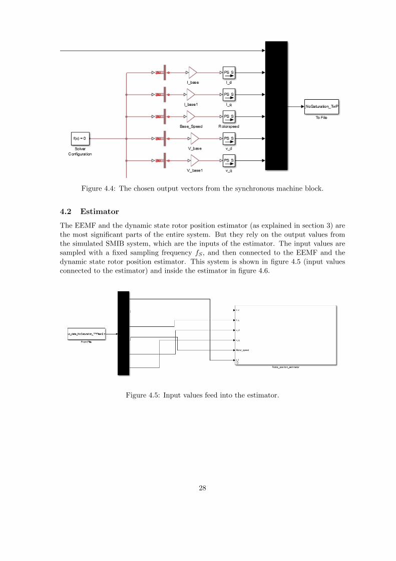
The output vectors should represent the three phase stator voltages and currents, alongwith the field current. Since the SimPowerSystems synchronous machine block only out-puts dq0 quantities, the actual rotor position is needed in order to obtain the abc or α-βcomponents. The rotor position is not an output vector and thus it has to be obtainedfrom the rotor speed. The conversion from dq0 to α-β components is done in the sameSimulink file where the estimator is located at. This choice was done arbitrarily to ex-clude further configurations for the simulation. As seen in figure 4.4 the chosen outputvectors are converted from per unit quantities to their physical quantities. This was alsoan arbitrary choice due to the EEMF estimator using physical quantities.
27
Figure 4.4: The chosen output vectors from the synchronous machine block.
4.2 Estimator
The EEMF and the dynamic state rotor position estimator (as explained in section 3) arethe most significant parts of the entire system. But they rely on the output values fromthe simulated SMIB system, which are the inputs of the estimator. The input values aresampled with a fixed sampling frequency fS , and then connected to the EEMF and thedynamic state rotor position estimator. This system is shown in figure 4.5 (input valuesconnected to the estimator) and inside the estimator in figure 4.6.
Figure 4.5: Input values feed into the estimator.
28
Figure 4.6: The estimator function blocks, where the dq-αβ transform is marked with red,the sampling blocks in blue, the estimator blocks in green and computing the actual rotorposition in magenta.
Considering figure 4.5, the input values are loaded from a file and connected to a demulti-plexer block, which splits the different input values to be feed into the estimator. In figure4.6, the d- and q-axis currents and voltages are converted into α-β components beforesampling (marked with a red square) with the help of the actual rotor speed, which rep-resent the two-phase equivalent values which can be measured. As mentioned previously,the Simulink application SimPowerSystems only outputs dq components.
The actual rotor speed is the integral of the output rotor speed. To limit the rotor positionwithin the range [−π, π] the rotor speed after it is integrated is separated into its sineand cosine values, where the rotor position is then calculated with the help of the arctan2function. This will limit the rotor position within this interval and is necessary in order tocalculate the estimated rotor position error.
All input values are sampled, except the actual rotor speed where the actual rotor po-sition is obtained by the integrator. The rotor position is used for obtaining the rotorposition error by subtracting the actual rotor position from the estimated. The EEMF andthe dynamic estimators are marked with green.
4.2.1 Designing the EEMF subsystem
The EEMF system is based on equation (3.11) for solving the EEMF terms.
29
Figure 4.7: EEMF based rotor position estimator.
The current derivative is solved by using the backward Euler’s method. As shown in figure4.7 the [k − 1] sample is obtained from the delay block. The current as sample k − 1is subtracted from the current at sample k and then divided by the sampling time Ts.However the multiplication of Ld and the division of Ts are done simultaneously at thegain blocks Ld/Ts. The rotor angular speed is represented as a constant input value of thebase angular speed, which is a valid assumption in steady state. The final step consists ofsolving equation (3.12) from the equivalent EEMF terms.
4.2.2 Designing the dynamic state rotor position estimator
The dynamic state rotor position estimator is the most complex part, hence it will benecessary to explain the design in different parts, rather than explaining the function asa whole. The first part is where all the initial values are defined. The initial values aredefined when the difference of the field current at sample k and k−1 reaches a certain value.To compensate for the loss of accuracy during this initial dynamic state, the input valuesare calculated by using a previous rotor position value and then predicted by assuming therotor speed maintains its constant steady state value during the beginning of the dynamic
30
state.
Figure 4.8: Initial dynamic state observer (green), Initial state estimation (blue) and theestimated rotor speed from the EEMF (red).
In the blue region in figure 4.8, the initial d-axis current is estimated with the help ofequation (3.15), assuming the d-axis damper winding current is zero. The initial dynamicstate is detected by the configuration shown in the green region. Since the differencebetween the field winding current at the current and previous sample is not exactly zero atsteady state, thus the dynamic state boundary for the current difference is chosen arbitrarilyat a certain level. As seen in figure 4.8, the dynamic state rotor position estimator isactivated for current difference values higher than 0.0001 pu. During this case the switchconnects the output to the uppermost input and thus integrates a positive value. Theintegrator is floored at zero, so that the output is limited to a digital output signal of 0and 1. Any positive value at the output of the integrator will generate an output signalas 1. When the current difference is below the boundary value, the switch will connectthe output to the second port, which is connected to a constant negative value. Theoutput value from the integrator will decrease until it reaches zero, thus the dynamic staterotor position estimator will be switched off after a certain amount of time. The currentdifference will reach values under the boundary limit for short periods of time, therefore itis necessary to have a lower constant negative input value to make sure the output valuedoesn’t drop to zero during a period of dynamic operation.
31
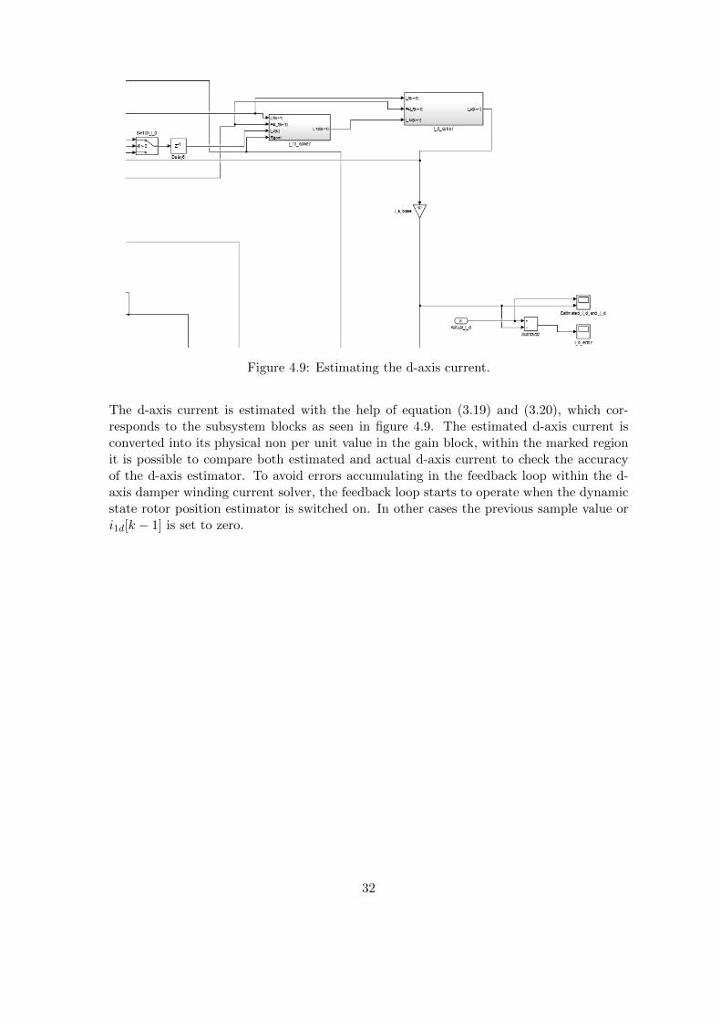
Figure 4.9: Estimating the d-axis current.
The d-axis current is estimated with the help of equation (3.19) and (3.20), which cor-responds to the subsystem blocks as seen in figure 4.9. The estimated d-axis current isconverted into its physical non per unit value in the gain block, within the marked regionit is possible to compare both estimated and actual d-axis current to check the accuracyof the d-axis estimator. To avoid errors accumulating in the feedback loop within the d-axis damper winding current solver, the feedback loop starts to operate when the dynamicstate rotor position estimator is switched on. In other cases the previous sample value ori1d[k − 1] is set to zero.
32
Figure 4.10: Detecting the correct solution from the two calculated rotor positions fromthe d-axis current.
The red marked region in figure 4.10 is the entire system of detecting the right solutionbetween equation (3.23) and (3.24). The green arrow points out where the output valueof equation (3.23) is located. Similarly the blue arrow points out where the output ofequation (3.24) is. The system which solves the inequality (3.25) is in the magenta region.
As mentioned previously in section 3.2.2 the estimated rotor position will experience inac-curacies when the q-axis current is close to zero. The integrating part which functions byintegrating from the initial rotor position with an angular rotor speed assumed to be therated angular speed, when the q-axis current gets close to zero, along with a high derivativeof the rotor position. Figure 4.11 shows the input ports to the integrating part. Figure4.12 is the inside of the subsystem of the integrating part.
33
Figure 4.11: Input values for the integrating part.
Figure 4.12: Integrating part.
The output from the corrected rotor position estimation is feed into a block that switchesthe dynamic state rotor position and the integrator. The other is feed into an speed observer(marked in red) which purpose is to detect high or low rotor speeds below rated speed.The green region includes the predicted q-axis current and the inequality (3.27) withinthe magenta colored region. Since the estimated rotor position at sample k is unknown, apredicted rotor position at sample k is used instead. The integrator is shown in the blueregion and consists of an initial rotor position detector and the integrator itself. To avoid
34
large initial value errors, the initial rotor position is predicted from previous sample values.For this case from the previous 5 samples or k− 5 samples, which gives a predictor term of5 · ωbase. When the inequality is less than ”a” the predicted rotor position is continuouslyupdated in the sample and hold block. At the moment when the inequality is higher than”a” the switching signal for the sample and hold block is zero, hence the rotor positionmaintains a constant value which is equal to the last sample value when the input signalwas one. This serves as the constant term θre[k
′] in equation (3.26). When the integratingpart is switched off, the input for the integrator is switched to a constant negative value,high enough to drive the output value quickly to zero (where the minimum output valuefrom the integrator is set to zero).
4.2.3 Calculating the rotor position estimation error
Figure 4.13: Calculating the rotor position error.
To determine if the estimated rotor position is accurate it has to be compared to the actualrotor position. Since the estimated rotor position is a discrete quantity, for conveniencethe actual rotor position were sampled as well, in order to reduce the in between sampleerrors. If necessary the estimated rotor position could be reconstructed to generate a nondiscrete output value. In figure 4.13 the subsystem in the green area is where the actualrotor position is sampled, the red area is the EEMF based rotor position estimation, theblue is the dynamic state rotor position estimator. To compare the performance betweenthe different steps of how to estimate the rotor position, from top to bottom in the right offigure 4.13, only the EEMF estimator is used, then with the included dynamic state rotorposition estimator and the final step of estimating the rotor position error.
35
5 Results and discussion
5.1 Input data
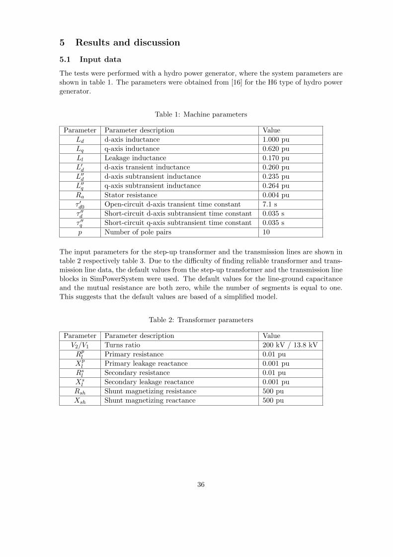
The tests were performed with a hydro power generator, where the system parameters areshown in table 1. The parameters were obtained from [16] for the H6 type of hydro powergenerator.
Table 1: Machine parameters
Parameter Parameter description Value
Ld d-axis inductance 1.000 pu
Lq q-axis inductance 0.620 pu
Ll Leakage inductance 0.170 pu
L′d d-axis transient inductance 0.260 pu
L′′d d-axis subtransient inductance 0.235 pu
L′′q q-axis subtransient inductance 0.264 pu
Ra Stator resistance 0.004 pu
τ ′d0 Open-circuit d-axis transient time constant 7.1 s
τ ′′d Short-circuit d-axis subtransient time constant 0.035 s
τ ′′q Short-circuit q-axis subtransient time constant 0.035 s
p Number of pole pairs 10
The input parameters for the step-up transformer and the transmission lines are shown intable 2 respectively table 3. Due to the difficulty of finding reliable transformer and trans-mission line data, the default values from the step-up transformer and the transmission lineblocks in SimPowerSystem were used. The default values for the line-ground capacitanceand the mutual resistance are both zero, while the number of segments is equal to one.This suggests that the default values are based of a simplified model.
Table 2: Transformer parameters
Parameter Parameter description Value
V2/V1 Turns ratio 200 kV / 13.8 kV
Rpl Primary resistance 0.01 pu
Xpl Primary leakage reactance 0.001 pu
Rsl Secondary resistance 0.01 pu
Xsl Secondary leakage reactance 0.001 pu
Rsh Shunt magnetizing resistance 500 pu
Xsh Shunt magnetizing reactance 500 pu
36
Table 3: Line parameters
Parameter Parameter description Value
R Line resistance 0.02 Ω/km
L Line inductance 0.5 mH/km
M Mutual inductance 0.1 mH/km
Cl Line-line capacitance 0.3µF/km
Cg Line-ground capacitance 0µF/km
Rm Mutual resistance 0 Ω/km
Rp Parasitic series resistance 1µΩ/km
Gp Parasitic parallel conductance 1µS/km
Ns Number of segments 1
The estimator input data are the same as the values presented in table 1, except the othercircuit parameters have been determined by the time constants, transient and subtransientinductances. The machine parameters derived from the given time constants, transient andsubtransient inductances are refered to appendix A.2. As for the constants for equation(3.25) and the integrating part in equation (3.27), the constant values were chosen as follows
ε = 10, a = 6, b = 60, c = 10
Other input data included the initial conditions for the synchronous generator, step uptransformer and the infinite bus. The choice of initial can be chosen so that the syn-chronous generator starts from a steady state condition. As long as the system convergesto a steady state relatively fast, it is not necessary to make the work more complicated inorder to stabilize the system at start. The initial values were chosen by trial an error tomake the system stable enough for it to converge fast. The initial conditions are shown intable 4.
Table 4: Initial conditions
Type Parameter description Value
Generator Terminal voltage magnitude 13.80 kV
Generator Terminal voltage angle 0 deg
Generator Terminal active power 0.5 pu
Generator Terminal reactive power 0 pu
Transformer Initial primary currents [53.8558,−53.8558, 0] A
Transformer Initial secondary currents [107.7116,−53.8558,−53.8558] A
Transformer Initial magnetizing currents [0, 0, 0] A
Transformer Initial fluxes [0, 0, 0] Wb
5.2 Simulation results
The simulations were carried out for a maximum of 15 seconds. During start, the generatorstarts from a non steady state operation, over time it will settle down to steady stateoperation. Three different cases of faults consisting of line-to-ground, phase-to-phase and
37
three phase fault were considered when running the simulation. The faults were generatedat t = 13 s where after 50 ms from the beginning of the fault line 2 is disconnected by thecircuit breakers. The purpose is to check how the rotor position estimator will react fordifferent types of faults and how accurate the estimated rotor position is.
5.2.1 Single-phase-to-ground fault
The phase-to-ground fault occurs from phase a to ground as shown in figure 5.1.
Figure 5.1: Illustration of a single-phase-to-ground (P-G) fault.
From the EEMF based method, the resulting rotor position error is shown in figure 5.2.During start the stator and rotor quantities are not at their steady state levels, hencewhy the estimation error is very high. Subsequently when the system has converged tosteady state, the error maintains a very low level, which is shown more in detail in figure5.4 with the included dynamic state rotor position estimator before fault. As observedat t = 13 s, the fault will cause the system to go into non steady state, hence why theerror during the fault is very high, which after clearing the fault quickly reaches steadystate. The dynamic state rotor position estimator is set to operate at t > 12 s, in order toavoid it to operate at start. The resulting rotor position estimation error with the includeddynamic state rotor position estimator is shown in figure 5.3. For t = 13 s when the faultoccurs there is a very small change in the rotor position error. A closeup between thefault intervall figure 5.4 shows clearly how the error behaves during pre-fault, during faultand post fault. During pre fault at steady state operation, the estimated rotor positionerror oscillates with an amplitude of approximately 0.001 rad/s, observed between 12 and 13seconds. This is observed to be caused by the step up transformer, as mentioned previously.During fault there are positive and negative error spikes present, these correspond to theinaccuracies caused by the q-axis passing the zero boundary. At the peak values of thespikes the integrator is switched on, otherwise they would continue up to very high values.During post fault (after the fault is cleared) the system is stabilizing and the estimatedrotor position error maintains a steady value. When the dynamics of the field current hasmaintained low values, the dynamic state rotor position estimator is switched off, as seenaround t = 13.65 s.
38
Figure 5.2: Rotor position estimation error for a P-G fault without the dynamic state rotorposition estimator.
Figure 5.3: Rotor position estimation error for a P-G fault without the dynamic state rotorposition estimator.
39
Figure 5.4: Rotor position estimation error for a P-G fault with the dynamic state rotorposition estimator.
Figure 5.5: Rotor position estimation error for a P-G fault with the dynamic state rotorposition estimator (close to fault).
5.2.2 Phase-to-phase fault
For this case the phase-to-phase (or line-to-line) fault occurs from phase a to b as shownin figure 5.4.
40
Figure 5.6: Illustration of a phase-to-phase (P-P) fault.
Considering the case for the single-phase-to-ground fault, during fault the shape of theestimation error as function of time displayed an high frequency oscillation, combined withspikes or pulses. The same form can be observed in the phase-to-phase fault as shown infigure 5.8. The difference is the larger spikes during a fault, which suggests that the q-axiscurrent not only passes through the zero boundary for the peak value to reach a relativelyhigh negative value, but the peak value to reach relatively close to the zero boundary. Thed- and q-axis currents as a function of time is referred to the appendix.
During post fault the offset error is larger than that of the single-phase-ground fault.The reason might be due to a larger error when estimating the initial value for the d-axis damper winding current. The initial d-axis current should not make that much of adifference since it is based on a predicted value from a previous sample data.
Figure 5.7: Rotor position estimation error for a P-P fault without the dynamic state rotorposition estimator.
41
Figure 5.8: Rotor position estimation error for a P-P fault without the dynamic state rotorposition estimator.
Figure 5.9: Rotor position estimation error for a P-P fault with the dynamic state rotorposition estimator.
42
Figure 5.10: Rotor position estimation error for a P-P fault with the dynamic state rotorposition estimator (close to fault).
5.2.3 Three-phase-fault
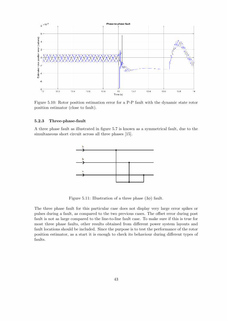
A three phase fault as illustrated in figure 5.7 is known as a symmetrical fault, due to thesimultaneous short circuit across all three phases [15].
Figure 5.11: Illustration of a three phase (3φ) fault.
The three phase fault for this particular case does not display very large error spikes orpulses during a fault, as compared to the two previous cases. The offset error during postfault is not as large compared to the line-to-line fault case. To make sure if this is true formost three phase faults, other results obtained from different power system layouts andfault locations should be included. Since the purpose is to test the performance of the rotorposition estimator, as a start it is enough to check its behaviour during different types offaults.
43
Figure 5.12: Rotor position estimation error for a 3φ fault without the dynamic state rotorposition estimator.
Figure 5.13: Rotor position estimation error for a 3φ fault without the dynamic state rotorposition estimator.
44
Figure 5.14: Rotor position estimation error for a 3φ fault with the dynamic state rotorposition estimator.
Figure 5.15: Rotor position estimation error for a 3φ fault with the dynamic state rotorposition estimator (close to fault).
5.3 Discussion
5.3.1 Choice of power system model
The choice of simulation environment for the power system was done to make it behaveas realistically as possible. Such a system would be incredibly complicated and futile ifaccurate results can be achieved from a much simpler system. The simulation environmentwas designed in Simulink with the help of the built in package ”simpowersystems”. Ascompared to a real system, the salient pole synchronous generator was modeled on theclassical system and a simple field saturation model. Hence, if further tests were to beperformed considering the effects of saturation, an analysis should be made to determine
45
if a more detailed saturation model will be necessary in order to obtain more realisticresults. The type of step up transformer commonly used between a generator and thetransmission network is of the ∆−Y type, which was the most important considerationwhen choosing the right transformer model. Although the transformer block from theSimPowerSystems was an ideal transformer model in the sense that the effects of iron coresaturation were neglected. However the model did consider non-ideal properties such asleakage inductance, eddy currents etc. The notion that a large power system network canbe represented as a constant ac voltage source, hence an infinite bus saves a lot of timeand reduces computational effort to run such a system.
5.3.2 Choice of estimator model
The most difficult part of this thesis was the choice of the right type of estimator design,best adapted to a salient pole synchronous generator. A lot of studies have been made toestimate the rotor position for a permanent magnet synchronous machine, with no presenceof damper windings. This is the reason why the choice of estimation model was difficultfor a more complicated synchronous generator. A lot of effort went to directly estimatingthe rotor position from the known machine parameters and the measured rotor and statorcurrents and voltages. The final choice was to split the estimator into two parts, the firstone considering steady state operation and the second one using the initial values fromthe first estimator to solve a set of differential equations to calculate the d-axis current,which contains the information of the rotor position. This was not enough considering thatby calculating the d-axis current by itself would yield two different solutions to the rotorposition. The method was to analyze the behavior of the rotor speed, for both solutionsand chose the one that gave the most reasonable behavior for a synchronous generator,regarding its rate of acceleration and angular speed. For a generator with high inertia,rapid accelerations should not be expected. For a machine connected to the power system,a speed close to the rated speed is expected, unless during a case when the synchronousmachine loses synchronism, then higher rotor angular speeds are expected.
46
6 Conclusion and future work
6.1 Conclusion
The results from the three cases of line faults shows that the rotor position is improvedtremendously with the added dynamic state rotor position estimator for all three differenttypes of faults, with the effects of saturation disabled. The EEMF based rotor positionestimator worked well during steady state operation, however the intended purpose fromthe beginning was to estimate the rotor position for both steady-state and dynamic cases,which turned out to be impossible due to the present d-axis field and damper windingcurrent dynamics, along with the q-axis damper winding current. A much simpler methodfor estimating the rotor position could have been utilized, but due to the versatility of theEEMF method it was used instead, presumably since it is independent of the d and q axiscurrent dynamics. The dynamic state rotor position estimator could have been made evenmore accurate by adjusting the integrating setting constants to more optimal values. Asseen for the phase to phase fault there are still instances when the initial rotor positionduring the integrating phase has a relatively high error. An another method to improve theestimation of the initial values for the dynamic state rotor position estimator is to make itoperate before a fault occurs. An another possible method is to start estimating the d-axiscurrent from previous sample data to the current sample data, within the sampling timeinterval from the time the dynamic state rotor position estimator starts to operate. Dueto the time constraint, any further improved estimator designs/models were not consid-ered. More details on how to make the rotor position estimation more suited for practicalapplications will be discussed in Future work.
6.2 Future work
As an continuation with the current estimator design, the most important addition is toinclude a method for estimating the d-axis mutual inductance to account for the effects ofsaturation. If it is necessary, other methods could be chosen to estimate the rotor positionwhich are more suitable for taking the effects of saturation into account. Further it couldbe useful to only limit the use for a sensor-less rotor position estimator for only a certaincases. As example the rotor position could be estimated during normal operation only,hence assuming that the rotor position should only operate when no faults occurs close tothe synchronous generator. What this implies is that the rotor position should not only beestimated during steady state operation, but during power swings from other generatorsor machines close to the generator from which the rotor position is estimated.
There is also a possibility for estimating the load angle with the swing center voltagemethod. The load angle could be proven useful for estimating the rotor position.
47
Appendix A
A.1 Per Unit System for Stator and Rotor Quantities
es,base =11267.7 V
is,base =2070.82 A
fbase =60 Hz
ωbase =2πfbase
Zs,base =es,baseis,base
Ls,base =Zs,base
ωbase
Ψs,base =Ls,baseis,base =es,baseωbase
ifd,base =1300 A
efd,base =13.5926 V
A.2 Derived Standard parameters from time constants
The following parameters are derived from (2.87) with the classical expression
Lfd =0.1009 pu
L1d =0.2342 pu
Rfd =3.4779 · 10−4 pu
R1d =0.0222 pu
L11d =Lad + L1d pu
48
Appendix B
B.1 Complementary results for P-G fault
Figure B.1: Measured field current ifd in per-unit.
Figure B.2: Estimation error for the d-axis current [A] rms.
49
Figure B.3: Predicted q-axis current [A] rms.
B.2 Complementary results for P-P fault
Figure B.4: Measured field current ifd in per-unit.
50
Figure B.5: Estimation error for the d-axis current [A] rms.
Figure B.6: Predicted q-axis current [A] rms.
B.3 Complementary results for 3φ fault
51
Figure B.7: Measured field current ifd in per-unit.
Figure B.8: Estimation error for the d-axis current [A] rms.
52
Figure B.9: Predicted q-axis current [A] rms.
53
Appendix C
C.1 Calculating id and i1d in Simulink
Figure C.1: Calculating the d-axis damper winding current i1d.
Figure C.2: Calculating the d-axis stator current id.
C.2 Other Simulink systems
54
Figure C.3: dq to α− β transform.
Figure C.4: α− β to dq transform.
55
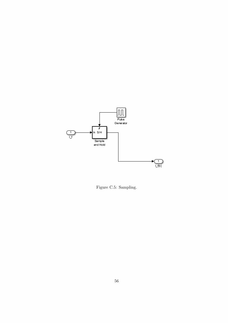
Figure C.5: Sampling.
56
Appendix D
D.1 Magnetic saturation
The model used in [14] to account for the effects of saturation is based on the followingassumptions.
1. Leakage inductances are independent of saturation
2. Leakage fluxes do not contribute to the iron saturation.
3. The saturation relationship under loaded conditions is the same as under no-loadconditions. Hence the open-circuit saturation curve can be used to simulate theeffects of saturation.
4. There is no magnetic cross coupling between the d- and q-axes.
5. Saturation effects for the quadrature axes are neglected, due to a salient pole rotorhaving a larger air gap at the q-axis.
From the above assumptions, only the d axis inductance is affected by saturation. Hencethe effects of saturation is modeled as
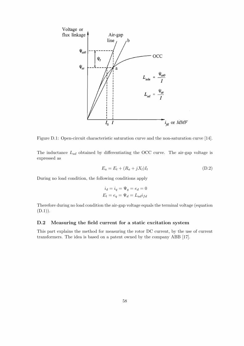
Lad = KsdLadu (D.1)
whereKsd is the saturation factor and Ladu is the unsaturated value of Ladu. The saturationfactor is a function of the d- and q-axis flux linkage Ψat, where the saturation factor curveis obtained from the open-circuit characteristics (assumption 3). Under no load conditions,the open circuit characteristics curve is obtained by expressing the air-gap voltage Ea as afunction of field current ifd, in per unit the air gap voltage is equal to the flux linkage Ψat.During OCC the air gap voltage is equal to the terminal voltage, which makes it possibleto express Lad as a function of the flux linkage.
57
Figure D.1: Open-circuit characteristic saturation curve and the non-saturation curve [14].
The inductance Lad obtained by differentiating the OCC curve. The air-gap voltage isexpressed as
Ea = Et + (Ra + jXl)It (D.2)
During no load condition, the following conditions apply
id = iq = Ψq = ed = 0
Et = eq = Ψd = Ladifd
Therefore during no load condition the air-gap voltage equals the terminal voltage (equation(D.1)).
D.2 Measuring the field current for a static excitation system
This part explains the method for measuring the rotor DC current, by the use of currenttransformers. The idea is based on a patent owned by the company ABB [17].
58
Figure D.2: Structure of a static excitation system, together with a current measuringdevice [17].
The idea is illustrated in figure D.2, where a three phase signal port is connected to anexternal IED (intelligent electronic device) is connected between the secondary side of therotor excitation transformer and the thyristor bridge. Alternatively between the stator andthe primary side of the excitation transformer.
The dc side current denoted as IDC is calculated from the following equation
IDC =| Ia | + | Ib | + | Ic |
2(D.3)
59
References
[1] Y. Zhao, Z. Zhang, W. Qiao, et al. “An Extended Flux Model-Based Rotor PositionEstimator for Sensorless Control of Salient-Pole Permanent-Magnet Synchronous Ma-chines”. In: IEEE Transactions on Power Electronics 30.8 (Aug. 2015), pp. 4412–4422. issn: 0885-8993. doi: 10.1109/TPEL.2014.2358621.
[2] Zhiqian Chen, M. Tomita, S. Doki, et al. “An extended electromotive force modelfor sensorless control of interior permanent-magnet synchronous motors”. In: IEEETransactions on Industrial Electronics 50.2 (Apr. 2003), pp. 288–295. issn: 0278-0046. doi: 10.1109/TIE.2003.809391.
[3] Y. Lee, Y. C. Kwon, and S. K. Sul. “Comparison of rotor position estimation per-formance in fundamental-model-based sensorless control of PMSM”. In: 2015 IEEEEnergy Conversion Congress and Exposition (ECCE). Sept. 2015, pp. 5624–5633.doi: 10.1109/ECCE.2015.7310451.
[4] Y. Zhao, Z. Zhang, W. Qiao, et al. “An extended flux model-based rotor positionestimator for sensorless control of interior permanent magnet synchronous machines”.In: 2013 IEEE Energy Conversion Congress and Exposition. Sept. 2013, pp. 3799–3806. doi: 10.1109/ECCE.2013.6647204.
[5] J. Liu, T. A. Nondahl, P. B. Schmidt, et al. “Rotor Position Estimation for Syn-chronous Machines Based on Equivalent EMF”. In: IEEE Transactions on IndustryApplications 47.3 (May 2011), pp. 1310–1318. issn: 0093-9994. doi: 10.1109/TIA.2011.2125935.
[6] Chuanyang Wang and Longya Xu. “Investigation of a practical approach for rotorposition estimation of PM machines without rotor saliency”. In: Power Electronicsand Motion Control Conference, 2000. Proceedings. IPEMC 2000. The Third Inter-national. Vol. 1. Aug. 2000, 329–335 vol.1. doi: 10.1109/IPEMC.2000.885424.
[7] M. J. Corley and R. D. Lorenz. “Rotor position and velocity estimation for a salient-pole permanent magnet synchronous machine at standstill and high speeds”. In:IEEE Transactions on Industry Applications 34.4 (July 1998), pp. 784–789. issn:0093-9994. doi: 10.1109/28.703973.
[8] R. V. Jacomini and E. Bim. “Sensorless rotor position based on MRAS observer fordoubly fed induction generator”. In: 2015 IEEE 13th Brazilian Power ElectronicsConference and 1st Southern Power Electronics Conference (COBEP/SPEC). Nov.2015, pp. 1–6. doi: 10.1109/COBEP.2015.7420139.
[9] M. Tomita, T. Senjyu, S. Doki, et al. “New sensorless control for brushless DC motorsusing disturbance observers and adaptive velocity estimations”. In: IEEE Transac-tions on Industrial Electronics 45.2 (Apr. 1998), pp. 274–282. issn: 0278-0046. doi:10.1109/41.681226.
[10] J. P. Johnson, M. Ehsani, and Y. Guzelgunler. “Review of sensorless methods forbrushless DC”. In: Industry Applications Conference, 1999. Thirty-Fourth IAS An-nual Meeting. Conference Record of the 1999 IEEE. Vol. 1. 1999, 143–150 vol.1. doi:10.1109/IAS.1999.799944.
60
[11] V. Hubik, M. Sveda, and V. Singule. “On the development of BLDC motor con-trol run-up algorithms for aerospace application”. In: Power Electronics and MotionControl Conference, 2008. EPE-PEMC 2008. 13th. Sept. 2008, pp. 1620–1624. doi:10.1109/EPEPEMC.2008.4635499.
[12] S. Morimoto, K. Kawamoto, M. Sanada, et al. “Sensorless control strategy for salient-pole PMSM based on extended EMF in rotating reference frame”. In: IEEE Trans-actions on Industry Applications 38.4 (July 2002), pp. 1054–1061. issn: 0093-9994.doi: 10.1109/TIA.2002.800777.
[13] S. Koonlaboon and S. Sangwongwanich. “Sensorless control of interior permanent-magnet synchronous motors based on a fictitious permanent-magnet flux model”. In:Fourtieth IAS Annual Meeting. Conference Record of the 2005 Industry ApplicationsConference, 2005. Vol. 1. Oct. 2005, 311–318 Vol. 1. doi: 10.1109/IAS.2005.
1518326.
[14] P. Kundur. Power System Stability and Control. McGraw Hill, 1994.
[15] H. Saadat. Power System Analysis. PSA Publishing, 2010.
[16] A. A. Fouad Paul M. Anderson. Power System Control and Stability. Wiley-IEEEPress, 2002.
[17] Z. Gajic, D. Trisic, and S. Roxenborg. “Rotor DC current measurement by utilizingcurrent transformers”. In: Developments in Power System Protection (DPSP 2014),12th IET International Conference on. Mar. 2014, pp. 1–6. doi: 10.1049/cp.2014.0023.