Page 1
Syndrome decoding of binary convolutional codes
Citation for published version (APA):Vinck, A. J. (1980). Syndrome decoding of binary convolutional codes. Eindhoven: Technische HogeschoolEindhoven. https://doi.org/10.6100/IR148801
DOI:10.6100/IR148801
Document status and date:Published: 01/01/1980
Document Version:Publisher’s PDF, also known as Version of Record (includes final page, issue and volume numbers)
Please check the document version of this publication:
• A submitted manuscript is the version of the article upon submission and before peer-review. There can beimportant differences between the submitted version and the official published version of record. Peopleinterested in the research are advised to contact the author for the final version of the publication, or visit theDOI to the publisher's website.• The final author version and the galley proof are versions of the publication after peer review.• The final published version features the final layout of the paper including the volume, issue and pagenumbers.Link to publication
General rightsCopyright and moral rights for the publications made accessible in the public portal are retained by the authors and/or other copyright ownersand it is a condition of accessing publications that users recognise and abide by the legal requirements associated with these rights.
• Users may download and print one copy of any publication from the public portal for the purpose of private study or research. • You may not further distribute the material or use it for any profit-making activity or commercial gain • You may freely distribute the URL identifying the publication in the public portal.
If the publication is distributed under the terms of Article 25fa of the Dutch Copyright Act, indicated by the “Taverne” license above, pleasefollow below link for the End User Agreement:www.tue.nl/taverne
Take down policyIf you believe that this document breaches copyright please contact us at:[email protected] details and we will investigate your claim.
Download date: 16. Apr. 2020
Page 3
SYNDROME DECODING OF BINARY CONVOLUTIONAL CODES
PROEFSCHRIFT
ter verkrijging van de graad van doctor in de
technische wetenschappen aan de Technische
Hogeschool Eindhoven, op gezag van de rector
magnificus, prof.ir. J. Erkelens, voor een
commissie aangewezen door het college van
dekanen in het openbaar te verdedigen op
dinsdag 26 februari 1980 te 16.00 uur
door
Adrianus Johannes Vinck
geboren te Breda.
@) 1980 by A.J. Vinck, Eindhoven, The Netherlands.
Druk: J. van Haaren b.v.
Page 4
DIT PROEFSCHRIFT IS GOEDGEKEURD
DOOR DE PROMOTOREN
Prof.dr.ir. J.P.M. Schalkwijk
en
Prof. R. Johannessen.
Page 5
aan Marty,
aan mijn moeder en
ter gedachtenis aan mijn vader.
Page 6
Contents.
Chapter I.
Chapter II.
Chapter III.
Chapter IV.
Introduction.
Syndrome former analysis for
rate (n-1)/n codes.
Algorithm.
Special R=(n-1)/n codes-metric/path
register savings.
9
16
27
Chapter v. Sequential decoding 33
Chapter VI. Simulation of the stack decoding algorithm. 41
Chapter VII. Channel model. 51
Chapter VIII. Two important distance measures. 56
Chapter IX. Truncation error probability. 65
Conclusions.
Acknowledgements.
References.
Abstract.
Curriculum vitae.
71
72
73
75
76
Page 7
I. Introduction.
This thesis concerns the decoding of convolutional codes. Two
new decoding methods are developed that are both making use of a
channel noise generated syndrome . The first decode r i s based on the
polynomial parity matrix HT, whereas the second one uses the matrix
(H-l)T, i.e. the transpose of the right inverse of H. Hence, the code
generator G does not play the prominent role that it does in conven
tional decoders. In the remainder of this Chapter we introduce some
mathematical notation that will be useful in the sequel. Chapter II
gives a description of the state space of the syndrome former. Using
this state space f ormalism, Chapters III and IV present a maximum
likelihood (ML) decoding algorithm that allows savings in the complex
ity of a Viterbi like syndrome decoder . The above results a re partly
given in [1) - [3]. Chapter V gives a class of codes that yields a n
improved performance in conjunction with sequential stack decoding.
In particular, the distribution of the number of computations per
i n formation frame is improved by an order of magnitude. The simulation
results of Chapter VI indicate that the memory size of a s tack d ecoder
can approxi mately be reduced by a fac tor of 5 . Chapter VI discusses
two distance measures that are important for both the ML decoder and
the sequential decoder. Chapter VII gives a more extensive view on the
channel model that is used throughout this thesis . We give a way to
u se cha nnel me asurement information in syndrome decoding. In
Chapter VIII we derive upper bounds on the error r ate of a Viterbi like
ML decoder with finite path register memory. These bounds a re compared
with simulation res ults.
Page 8
Fig. 1 shows a conventional [4) binary rate 2/3 convolutional
encoder with two memory elements. The inputs to this encoder are two
binary message sequences
< m.> l
i=l '2
The outputs are t!1ree binary codeword sequences <c1>, <c?, and <c
3>
(hence the rate is 2/3). The elements of the three output sequences
where $ denotes modulo-2 addition.
Fig. 1. Rate 2/3 convolutional encoder.
2
Page 9
We express the input and output sequences in terms of the
delay operator D :
m. (D) -1 •• •+ mi._1D + miD +
1.
2 i=1,2 milD + mi2D + ... ,
c. (D) -1 2
j =l ,2,) ••• + cj,-1D + cjO + cj 1D + cj 2D + ... , J
Fo r notational convenience we shall generally suppress the parenthetical
D in subsequent references to sequences; thus mi means mi (D),
c. c. (D) , a nd so forth, >~here the fact that a letter represents a J J
sequence (transform) should be clear from the context. The input/
/output relationships are expressed concisely as
£ mG
G = (g . . (D)] is l.J
D
and formal power series multiplication with coeffic ient operations
modulo-2 is applied . In genera l , there are k inputs and n outputs . If
we define the cons traint lengt h f or the i-th input as
\!. 1.
max [deg gij (Dl]
Page 10
then the overall constrain' ! 'r .. 1t.!·.
(v=2 for the encoder of Fig. 1) equals the number of memory elements
for what Forney [4] calls the obvious realization of the encoder. Note
that in the obvious realization there are as many shift registers as
inputs. If the number of shift registers is equal to the number of
outputs, then the realization is called adjoint obvious. Fig. 2
represents the adjoint obvious realization of the encoder of Fig. 1.
Fig. 2. Adjoint obvious realization of the encoder
of Fig. 1.
The dual code CJ_ to a convolutional code C, generated by an
encoder G, is the linear space generated by the set of all n-tuples
of finite sequences 'i.• such that the inner product (:!!,,x_l ~ ~·'j_T
(where T means transpose) is zero for all x in C. The dual code of
4
Page 11
a rate k/n convolutional code can be generated by a rate (n-k)/n
encoder H such that G•HT = O. The n-input, {n-k)-output linear
sequential circuit whose transfer function matrix is HT, is called a
syndrome former, and has the property that xHT Q. iff ~ E C . The
desired matrix HT can be obtained from the inverse of the B matrix
in an invariant factor decomposition [4] , G = AfB of the encoder
matri·x G by taking the last (n-k) columns of B-l. In [ 4], Forney also
proves that the first k rows of the matrix B generate the same code
as G.
For the encoder G of Fig. 1 we have an HT matrix
Fig. 3 and Fig. 4 give the obvious and adjoint obvious realization
<W>
'-~~~~~~~~~~~~~-<~>
Fig. 3. Syndrome former in obvious realization.
Page 12
<W:>
Fig. 4. Syndrome former in adjoint obvious realization.
of the syndrome former. Note that the realization of Fig. 4 requires
as many memory elements as does the encoder realization of Fig. 1.
Let G be a convolutional encoder represented by the first k
rows of a polynomial n x n - matrix B with polynomial inverse • If
we define to be fonned by the first k columns of B-1 , then
-1 xGG ~for all~· Sirnularely, for the last (n-k) rows (H-l)T of B,
and the last (n-k) columns HT of B-l we have y_(H-l)T = y_ for all 'i..:
Summarizing
B -1
B -1
BB -1
B B I . n
Let n be the error vector sequence generated by the channel,
and let !. = £ + ~be the received data vector sequence. Given r and
the estimate n Of the channel noise, one can form an estimate m Of the
6
Page 13
message vector as follows.
m + e + e
where ~ is defined as the message correction vector sequence estimate.
The syndrome vector sequence w is defined as
{:,. T w rH
T (~ + .!!_)H
T nH
The task of an ML decoder is now to find an error vector sequence
estimate !!_ of minimum Hamming weight that may be a cause of the
(la)
syndrome vector sequence ~· Chapter III gives a decoding method that
can be described in terms of the state space of the syndrome former HT
Note that
n -1
nB B -1 T
eG + ~(H ) • (lb)
Hence alternatively, in terms of (lb) we can formulate the ML decoding
-1 T algorithm as that of finding the codeword eG closest to ~(H ) . Then
the resulting message correction vector sequence estimate ~corresponds
again to a noise estimate !!_of minimum Hamming weight. Note that in
the classical Viterbi decoder the received data vector sequence
(!!!_G + .!!_) is compared with a possible transmitted codeword ~G, without
using the matrix [G-lHT].
For an additive white Gaussian noise channel (AWGN) with hard
quantization at the matched filter output, the previously mentioned
encoding and syndrome forming circuits, together with the invertor G-l,
7
Page 14
are used as indicated in Fig. 5.
Fig. 5. Possible decoder implementation.
8
Page 15
II. Syndrome former analysis for rate (n-1)/n codes.
The algorithm of Chapter III allows a description based on the
state space of the syndrome former. This is the subject of the present
Chapter. The syndrome former HT of a rate (n-1)/n code can be realized
in an adjoint obvious realization involving only one shift register of
length V • Fig. 6 illustrates the adjoint obvious realization for the
syndrome former HT, where H [ 1 + D + n2 , 1 + Dz , 1] •
Fig. 6. Adjoint obvious realization of a syndrome former.
The physical state of a linear sequential network such as the
syndrome former of Fig. 6 is defined as the contents o1
= [s1
, s2
,
'" , \!] of its memory elements. The abstract state is defined as the
output of the syndrome former in response to a sequence of all zero input
vectors. Hence, the physical state directly determines the abstract state.
States are denoted by lower case Greek letters with a subscript, e.g.,
9
Page 16
and its left shifts
a2 ~ [s2 t SJ ' ... ,
"' [s3 a3 t 54
and so on. occasionally, if sv
e.g.,
, O]
, 0 , O]
0 , we also write the right shift,
00
Fig. 7. State diagram of syndrome fonner.
10
Page 17
For a state space analysis, it is convenient to represent the
syndrome former of a rate (n-1)/n code by an n-tuple (A,B,C,•••,D) of
binary connection polynomials. The coefficients of A,B,C,•••,D are the
states generated by the system, and are denoted by
Without loss of generality we assume av= 1. This assumption is
justified by the definition of V and implies that the state space has
dimension v.
The syndrome digit w, and the new state T1
are completely
determined by the present,state cr1
and the noise vector [x,y,z,•••,t],
[x , y , z , ••• , t]
(2)
w
Fig. 7 gives the state diagram of the syndrome former of Fig. 6.
Solid lines correspond to a syndrome digit w O, and dashed lines
correspond to a syndrome digit w = 1. The decimal values indicated
along the edges are the noise vector and the message correction vector,
respectively, to be interpreted as binary numbers. 'The fact that the
message correction vector is solely determined by the next state of
11
Page 18
the syndrome former follows from Forney [5). He proves that the
inverter G-l can be constructed by a combinatorial network connected
to the memory elements of HT. Hence, the contents of these memory
elements, i.e. the physical state of HT, determines the output of G-l
Now consider the linear subspace L[a1
, $1
, y1
, ••• , o1
] spanned
by the generators a1
, S1 , y1 , ••• , o1 • If this subspace has
dimension q, then according to (2), each state a1
has exactly 2q state
transition images. Again by (2), these images form a coset of
o1
) • This coset will be called the "sink
tuple" of a 1 • To see, how many preimages a given state has, two
transitions to sink states are given below.
n = [x , y , z , ••• , t]
w
n 1 ;;;; [x' , y' , z 1
, ••• , t']
l a•t-=---1 "-....
T' 1
w' (3)
As a2
and crz have a rightmost component equal to zero, the noise vector
input n' must give rise to the same rightmost component as does!!• in
order for 'i• to equal -r 1 . In addition, for each possible!!', we can
find two possible states such that Ti = -r1
, i.e. two states that differ
12
Page 19
only in the leftmost component. Note that for av = 1, the vectors
S1 + b\IC!l 1 Yl + CVC!l , ••• , o1 + d\lal have a rightmost coordinate
equal to zero. Thus these vectors have a right shift. If we define
l1 El = [1,0,0, •••,O] as a row vector of length v, then dim L[a
1 , B1
y l , • • • , o1] = dim L(E l , (B+bva) O , (y+cva) O , • •• , (O+dva) 0]
and, hence, the state r1
has 2q preimages, i.e., all the states in the
coset· of L[E 1 , (S+bva) 0 , (y+cvaJ0
, ••• , (o+dva)0
] that contains
the preimage cr1
as is given in (3). This coset is called the "source
tuple" of r1
• It is easily verified that each element cr1
of a source-
tuple has the same sink-tuple.
It is this source/sink-tuple description of the state space
that will play an important rol in the remainder. To make things more
concrete we give a specific example for the syndrome former of Fig. 8.
Fig. 8. Syndrome former for the rate ~ convolutional code
with generator [l+D+D2+o
4 , l+D+D
4] .
Page 20
We have
al [1 0 1 ] 2 13
El [1 0 0 0] 2 8
131 [1 0 0 1 ] 2
9
(a+i3)o [O 0 0 l 2 2
Also,
Partition Source-tuples Sink-tuples
I { Q, 2, 8, 10} 0, 4, 9, 13}
II { 1, 3, 9,11} 2' 6,11,15}
III 4, 6,12,14} 1, 5, 8, 12}
IV 5, 7,13,15} 3, 7,10,14}
Fig. 9. shows a partition of the state space in source/sink-tuples.
Anticipating the results of Chapter IV, the states in Fig. 9 have
been geometrically arranged in such a way that the metric equivalence
classes {o} , {4} , {B} , {12} , {9,13} , {6,14} , {1,5} , {2,10} ,
and {3,7,11,15} are easily distinguishable. Two states that are in the
same metric equivalence class have the same metric value [ 7] , irrespe< -
tive of the noise vector sequence.
14
Page 21
source· tuples
I 11 I IV Ill
I
I 0 9 I 13 4 I I I
II 2 11 I 15 6 I
- -------+---"""'---10 3
I 7 14 IV I I
\\J 8 1 i 5 12 I I
Fi . 9. State space partition in source/sink-tuples for the
code of Fig. 8.
15
Page 22
III. Algorithm.
Given the syndrome sequence of a rate (n-1)/n code the
estimator must determine the state sequence that corresponds to a
noise vector sequence estimate of minimum Hamming.eight that may be
a possible cause of the syndrome sequence. As the estimation algorithm
to be described in this section is similar to Viterbi's [7], we can ~e
very brief. To find the required state sequence we introduce the
concept of a "metric function". A metric function is defined as a
nonnegative integer-valued function on the states. With every state
transition we now associate the Hamming weight WH of its noise vector
[x , y , ••• , t]
PROBLEM: Given a metric function f and a syndrome digit w,
find a metric function g that is state-wise minimal, and for every
state is consistent with at least one of the values of f on its
preimages under syndrome digit w, increased by the weight of its
corresponding state transition. The solution to this problem expresses
g in terms of f and w and can be formulated in terms of the source/
/sink-tuples of Chapter II. In fact, the values of g on a sink-tuple
Ti are completely determined by the values of f on the corresponding
source-tuple Si and by the syndrome digit w. The equations that
express g in terms of f and ware called "metric equations". They have
the form
[x,y,z, • • • ,t]
' I o1~'1 }. \
w (4)
16
Page 23
The particular preimage cr1
in (4) that realizes the minimum is called
the "survivor". When there are more preimages for which the minimum is
achieved: one could flip a multi-coin to determine the survivor.
However, we will shortly discover that a judicious choice of the
survivor among the candidate preimages offers the possibility of
significant savings in decoder hardware. The constructions of (4) can
be repeated, i.e., starting with a metric function f0
, given a
syndrome sequence w1
, w2
, w3
, • • •, one can form a sequence of metric
functions f 1 , f2
, f 3 , •••, iteratively by means of the metric equations.
The metric function fs' whose value fs(cr 1) at an arbitrary state cr1
equals the Hamming weight of the lightest path from the zero-state to
cr1
under an all-zero syndrome sequence w1
,w2
,w3,•••, = 0,0,0,••• , is
called the "stable metric function". It has the property
w = 0
Note that
f s
w 0
In order to make things more concrete we now give a specific example.
Fig. 10 represents one section of the trellis diagram [7] corresponding
to the state diagram of Fig. 7. From Fig. 10 we find for the metric
equations:
17
Page 24
g(O) w min [f(O), f(l) + 2 f(2) + 1 f 3) + 3]
+ w min [f (0) + 1 f (1) + 3 f(.2) f(3) + 2] (5a)
g(l) w min [f(O) + 2 , f (1) + 2 , f(2) + 1 , f (3) + 1]
+ w min (t(O) + 1 , f (1) + 1 ' f(2) + 2 , f (3) + 2]
(5b)
g(2) w min [f(O) + 2 , f ( 1) , f (2) + 3 ' f (3) + 1]
+ w min [f(O) + 3 ' f (1) + 1 , f(2) + 2 ' f(3)] (5c)
g(3) w min [f(O) + 2 , f(l) + 2 , f(2) + 1 , f(3) + 1}
+ w min [f(O) + 1 , f (1) + 1 , f (2) + 2 , f(3) + 2]
(5d)
"""]
Fig. 10. One section of the trellis diagram.
where w 1 - w. Note that for each value w 0 or w _;_ four arrows
18
Page 25
impinge on each image Tl. The preimage cr1 associated with the minimum
within the relevant pair of brackets in (5) is the, survivor. The case
where we have more candidates for a survivor among the preimages will
be considered shortly.
In the classical implementation of the Viterbi algorithm [7],
each state Tl (j) , j = 0,1,2,3 has a metric register MRj and a path
register PRj associated with it. The metric register is used to store
the current value of the metric function f. As only the differences
between the values of the metric function matter in the decoding
algorithm,
min {f[T1
(j)]}
0 ~ j ~ 3
is subtracted from the contents of all metric registers, thus bounding
the value of the contents of the metric registers. The path register
PRj stores the sequence of survivors leading up to state T1
(jl •
Observe that the right side of (5bl and (5d) are identical.
Hence the states Tl (1) and Tl (3) have identical metric register
contents. Moreover, selecting the identical survivor cr 1 in case of
a tie, Tl (1) and Tl (3) also have the same path register contents. The
metric register and the path register of either state T1 (1) or state
T1 (3) can be eleminated. Apparently certain symmetries in the state
space of the syndrome former can be exploited to reduce the amount
of decoder hardware. In the next Chapter we further explore this
possibility of reducing decoder hardware by introducing certain
19
Page 26
symmetries in the state space.
So far, the syndrome decoder has only been of theoretical
interest as a possible alternative to the classical Viterbi decoder.
We will now study a practical implementation. Using (5) we construct
Table I. The first column just numbers the rows of the Table. The
TABLE I
METRIC TRANSITIONS
1 w"' a w • l
old new ! new row number survivpr metrics
survivors metrics metrics
t___,
0 0 2 2 2 0 0 (0.ll 0 0 2 2 2 0 0 3 0 0 0 l 0
l 0 0 1 0 0 3 l 3 0 1 0 1 (0,2) (0,1) 3 (0, 11 l l 0 1
2 0 1 u 1 0 2 1 2 0 l 1 l 2 0 3 0 0 l l 1
J Q 1 1 l 0 (0,2,3) 1 (0 l,3) c 2 l 2 (0,2) 0 3 0 0 Q 0 0
• 0 2 1 2 0 (0,2) (0,1) (",2) 0 2 2 2 (0,2) 0 3 0 0 Q l 0
5 l l 0 1 (0,ZJ 2 2 0 0 0 0 2 !O, I ,2,J J {O, t ,2) 0 2 I 2
6 ;) 0 0 0 0 (2,3) l 12 ,3) Q 1 0 1 2 (0, ll J tO,U J l •c 1
PR[O 0·1] lgl ~
w PR[o 1:1 t- selector e tk·Dl ROM
l?I jm
I 0
OR
Fig. 11. Block diagram of the core of the syndrome decoder.
20
Page 27
second column lists all possible metric combinations f(O), f(l), f(2),
f(3). We start with the stable metric combination. As only the
differences between the metric values of a quadruple matter, we sub-
tract from each member of a quadruple the minimum value of the
quadruple, i.e., all quadruples of metrics in Table I have one or more
zeros. Columns 3 and 4 apply to the case that w = 0 and columns 5 and
6 to the case that w 1. Columns 3 and 5 list the survivors and
columns 4 and 6 the new metric values g(O), g(l), g(2) and g(3) as
given by (4). If there is a choice cf survivors, the candidates are
placed within parenthesis in the survivor columns.
Table I contains more information than is necessary for the
actual implementation of the syndrome decoder. As explained, knowledge
of the survivor leading to each state, together with the minimum
within each new quadruple of metric values, suffices to determine the
state sequence that corresponds to a noise vector sequence estimate
of minimum Hamming weight that may be a possible cause of the syndrome
s.equence. Bence, we omit the quadruples from Table I and store the
'fABLE II
CONTENTS OF THE ROM
., • 0 w"' 1
old ROM siurvivors new ROM U>dex gurv:l.vors r.ew ROM index address address jm address. l,.
0 0 0 (0,1) 0 0 0 0 0 3 0 1 (0, l ,3j
1 0 3 1 3 2 (0,2) (0,2) (0,ll 3 (0, ll 5 2
I 2 0 2 l 2 3 0 2 0 3 0 l 0
3 Q (0,2 ,3) 1 (0,2,3) • 0 (0,21 0 l 0 6 (0,1,2,3)
4 0 (0,2) (0, l) (0,2) 0 0 (0,2) 0 l 0 l 10, l ,J)
5 (0,2) 2 1 2 6 (0, 1,2' lJ 2 1011,:Z) 3 10, l,2) 4 0
I 6 0 (2, l) l (2 ,J} 2 {012) 2 (0t1) J 10,l) " (0,2)
'·--
21
Page 28
resulting Table II in a read-only memory (ROM.) • The operation of the
core part of the syndrome decoder can now be explained using the block
diagram of Fig. 11.
Assume that at time k the ROM address register AR contains
(AR) = 2 and the ROM data register DR contains (DR) (ROM,2). Note,
see Fig. 7 that thee-values to be shifted into PR0
[0:0) , PR1
[0:0),
PR2
[0:0], PR3
[0:0] arE!«0,0}, (1,1), (0,1), (1,0) respectively. Let
w = 1 at time t = k. Then according to row 2 and column 5 of Table II,
or according to the contents (DR) of the DR, replace
If,we let
PR0 [1 :D-1] - CONTENTS PR2[0:D-2]
PRl (1 ;D-1] - CONTENTS PR0[0:D-2]
PR2
[ 1 : D-1) - CONTENTS PR3
[ Q: D-2]
PR3
[1 :D-l] - CONTENTS PR0[0:D-2]
e(k-D) CONTENTS PRj(k)[D-l:D-1),
where j (k) minimizes MRj (k+l), i.e.,
MRj {k) {k+l) min MR. {k+l) J
then the selector determines e(k-d), using as j(k) the entry in row 2
and column 7, i.e. jm = 0, of Table II, which can also be found in
the DR. To complete the k-th cycle of the syndrome decoder, set
(AR) = 3 and read DR-{ROM,3).
22
Page 29
The ROM-implementation of the syndrome decod~r as described
above has been realized for the rate ~ codes listed in column 2 of
Table IIi. We will discuss some interesting aspects of the Table.
TABLE III
CODES REALIZED
code connection number of minumum distance number of total num-
polynomials; metric com- number of path paths at ber of as-0-th order right binations registers given dis- sociated
ta nee bit errors
101 12
111
10011 1,686 12
11011 12
10011 1,817
10111 10
10011 11,304 12
11101 12
Column 3 lists the number of metric combinations of the various codes.
The classical Viterbi decoder [7) can also be realized using a ROM
in the above manner. However, the Viterbi decoder for code has 31
metric combinations, whereas the syndrome decoder has only 12 metric
combinations. For the v = 4 codes this difference is even more
pronounced. For codes 2 and 3 the syndrome decoder has, respectively,
1686 and 1817 metric combinations, whereas the classical Viterbi
decoder for either of these codes has more than 15000 metric
combinations. Note that in columns 5, 6, and 7 both error events at
the free distance and error events at the free distance plus one are
considered. In a binary comparison with the no~rror sequence, an
error event at distance 2k has the same probability of occurrence
[8)as an error event at distance 2k - 1 , k = 1,2,•••. Thus, in the
case that the free distance is odd, error events at the free distance
23
Page 30
plus one should also be considered when comparing codes as to the bit
error probability Pb. Studying columns 5, 6, and 7 of Table III, we
observe that as far as the bit error probability is concerned code 4
is indistinguishable from codes 2 and 3. However, the syndrome decoder
for code 4 requires 11304 ROM-locations and code 4 is thus, from a
complexity point of view, inferior to codes 2 and 3.
The number of metric combinations increases rapidly with the
constraint length v of the code. Hence, for larger values of v the
size of the ROM in the implementation according to this Chapter soon
becomes prohibitive.
In 1978, Schalkwijk [9] used the ROM implementation to
construct a "metric x abstract state-diagram" in order to give an
exact evaluation of the error rate for ML decoders. This method of
calculating the error rate even applies to soft decisions. In soft
decision decoding not only a noise digit is hypothized to be either
0 or 1, but we have degrees of 0-ness, and 1-ness based on measurement
of the decision variable. This soft decision information increases
the number of rows in the ROM-·implementation and, hence, the number
of nodes in the metric x abstract state-diagram.
Reference [15] describes a coding strategy for duplex
channels that enables one to transfer the hardware of the program
complexity from the passive (receiving) side to the active (trans
mitting) side of the duplex channel. As pointed out in reference (15],
this coding strategy can be used to great advantage in a computer
network with a star configuration. For the information flow from the
24
Page 31
central computer to the satellites one us.es. the duplex strategy thus
only requiring one complex one-way decoder at the central facility.
For the information flow from a satellite computer towards the central
facility one uses one-way coding, again using the complex one-way
decoder at the central computer. One thus saves a nwnber of complex
one-way decoders equal to the nwnber of satellite computers in the
multiple dialog system (MDS). The duplex strategy [15] requires at
the active (transmitting) side of duplex channel an estimate of the
forward noise n1
. To form this estimate n1
, the data received at the
passive station are scrambled hy a convolutional scrambler g and sent
hack to the active station. At the active station one can now form
the estimate n1
using the Viterbi decoder for the "systematic"
convolutional code generated hy an encoder with connection polynomials
g1
= 1 , g2
= g. It is well known that "nonsystematic" convolutional
codes.are more powerful than systematic convolutional codes. With our
syndrome decoder we are now able fo find n1
according to a non
systematic code. To this end we modify the feedback-free scrambler
[15] into a feedback scrambler g2/g1, see Fig. 12. Note that w
Fig. 12. Duplex channel with. feedback scramblers.
25
Page 32
according to Fig. 12 is equal to n1
g2
+ . Hence, we can use our
syndrome decoder to obtain n1
• Fig. 13 gives the feedback scrambler
for the convolutional codes generated by G 2 2
ll+D I l+D+D ] •
y
Fig. 13. Feedback scrambler with g1
1+D+D2 •
Note that a syndrome former for a rate n-1/n code has n
input sequences and one output sequence. Thus the syndrome former
compresses n binary streams into one stream w and, hence, achieves
a data compression of a factor of n. The estimator part of the syndrome
decoder can with high probability of being correct recover the
original input sequence, given the compressed data sequence w. The
use of a syndrome decoder for data compression has also been studied
by Massey [16].
26
Page 33
IV. Special R = (n-1) /n codes""1l!etri.c/path register savings.
Without further ado we introduce the class rn,v,JI, of rate
(n-1)/n binary convolutional codes (A,B,c,•••,D) that exhibits the
state-space symmetries that will allow for an exponential reduction
of decoder hardware. The definition is that (A,B,C,•••,D)E rn,v,)1, if
and only if A ~ B, and
av
aj bj 0 ~ j ., i-1
a. bj , v-i+l ., j ~ v J
C,*••,D all have degree~ v-11,
gcd (A,B,c,··•,D) = 1 •
Conditions (6a) - (6c) and (6e) reduce to known sufficient conditions
for the rate ~ case. Condition (6d) will be discussed in Theorem 4.
The code of Fig. 3 is an element of r31211
, and the code of Fig. 8.
is an element of r214
,2
As a consequence of (6) we have
If condition (6e) is satisfied, then it follows from the invariant
(6a)
(6b)
(6c)
(6d)
(6e)
(7)
factor theorem [4] that then-tuple (A,B,C,•••,D) is a set of syndrome
polynomials for some noncatastrophic rate (n-1)/n convolutional code
(in fact, for a class of such codes).
Assume fn,v,,t F rp. For (A,B,C,•••,D)E fn,v,)1, an "i-singleton
state" is defined to be a state the last JI, components of which
27
Page 34
vanis.h. Linear combinations and left shifts of .!1.-singleton states are
also .!1.-singleton states. For every state $1
, the left shifts $i(i~J1.+1)
are .!!.-singleton states,. We state the following lemma and theorems
without proof.
Lemma : For every state cr1
, there exists a unique .!!.-singleton
state $.!1.+l and a unique index set I c{l,2,•••,.!1.} such that
a.. 1
Using this lemma, we now associate with the state cr1
the set [cr1
] (.!!.)
defined by
{$.!1.+l + E [a.i + ri (a.+tlli] lri E {0,1}, for all i}. iEI
Then we have the following theorem.
(8)
Theorem 2: The collection of all sets [cr1J (.!!.) forms a partition
of the state space.
Corollary: Based on the partition of the state space according
to Theorem 2, an equivalence relation Rn,v,.!1. can be defined where two
t t O d 0 1 11 d R ' 1 t iff [rl1
] (J!.) = frr1•] (J!.) s a es ·1 an 1 are ca e n,v,.!1.-equiva en v v
of The one-element equivalence classes of Rn,v,.!1. consist
exactly one .!!.-singleton state. Examples are the states O, 4, 8, and
12 in Fig. 9. The number Nn,v,.!1. of Rn,v,.!1.-equivalence classes can be
found as follows. First, take Ic {1,2,••.,J!.} in (8) fixed, and let
28
Page 35
J denote the cardinalLty of I, The last !I, components of an J!.~i;dngleton
v-.J!. j state are zero. H.ence there are 2 · J!.-singleton states. Now 2 of these
2v-J!. J!.-singleton states correspond to the same Rn,v, 2-equivalence class,
i.e. all J!.-singleton states differing by a linear combination of
{ ( 0 ) I . } h 2\1-J!.-j . l l f a+., i J. E. I • Hence t ere are Rn, \I, JI. -equi va ence c asses or
each I of cardinality j. Thus
2 E
j=O
Theorem 3: Let (A,B,C,•••,D) fn,v,J!.' and assume that
1 $JI.' $ 2. Then every Rn,v, 2-equivalence class of (A,B,c,•••,D) is a
union of Rn,v, 2 ,-equivalence class of (A,B,C,••o,DJ (see (7)).
In Fig. 9, we exhibit the R21412
-equivalence classes for the
syndrome former of Fig. 8. We claimed that any two states within the
same equivalence class have the same metric value irrespective of the
noise vector sequence. We are now ready to prove this result.
Theorem 4: Assume that (A,B,.C,•••,D)E.fn,v,2
• Let f0
be any
starting metric function, and let w1
, w2
, w3
; ••• be any syndrome
sequence. Then every iterate fu is constant on the Rn,v,u-equivalence
classes of (A,B,c,•••,D), 1 < u < JI,.
Proof: The proof is by induction on u. Consider the two
Rn,v,l-equivalent states ~ 2 + a 1 , and ~ 2 + $1
• Obviously they belong
to the same sink-tuple. We list their preimages, corresponding noise
vectors, and syndrome digits according to (3) in Table IV. We see
that on every line, i.e. for every preimage, the syndrome bits and
29
(9)
Page 36
Pre image
<P1 +zyo+ .. •+t<So
<P1 +{a.+Slo+zyo+•••+too
<P1+e1 +zyo+• .. +tllo
<P1+e1+{a+S)o+zyo+·••+t60
TABLE IV
<P2 +a.1
Noise;Syndrome <P2+fl1
Noise;Syndrome
T [0,1,z,""' 1 t] ;w
1 T
[1,0,z,•••,t] ;w1 T -[0,1,z,•••,t] ;w
1 [ T -1,0,z,•••,t] ;w
1
the Hamming weights of the state transitions t~ cp2
+ a.1
, and
and every w1• This proves the assertion for u: 1. Note that the
survivors for state <P2 + a. 1 and for state ~2 + S1
always can be chosen
in such a way, that they are identical. Thus roughly speaking, we need
one path register for each Rn,v, 1-equivalence class of states.
We now proceed by induction w.r.t. u. Let o1 and n1
be two
Rn,v,u+l-equivalent states that are not Rn,v,u-equivalent. Then
"' "' where I c {1,2,•••,u}. It is easy to find preimages o1
and n1
of o1
and n1 respectively, viz:
30
Page 37
cp +a + i: a. u+l u iEI\{l} i-1
(10)
"' "' "' "' Obviously o1
and n 1 are Rn,V,u-equivalent, thus ql and n 1 have the same
metric value. Furthermore, we observe that
+ t 0 if 1 i I
"' 01 = 02 if 1 E I al
+ l 0 if 1 i I "' n1 = n2
+ r 1 (a+Sl 1 if 1 E I al
Now consider the cosets Sand S' of L[E1
, (a+Sl0
, y0
, ••• , o0
] to
"' "' which o1
and n1
belong, respectively, and compare them element-wise.
The states
are obviously R -equivalent for all p,q,r,• .. ,sE{0,1}, since by n,v,u
the definition of El and by (6c), (6d) the last u components of
PE1 + q(a+Sl0
+ ry0
+•••+ so0
vanish. Furthermore, by (6b) we have
l: iEI
a, i
l: [ai + ri (ai+bil] iEI
Hence by (3) the preimages, in (10) give rise tc identical syndrome
31
Page 38
digits to an input vector [x , y , z , ••• , t] • These arguments
together however, imply that the values of fu+l on the corresponding
state transition images are equal, and hence fu+l is constant on the
Rn,v,u+l-equivalence classes. Furthermore, if a survivor for one state
in an Rn,v,u+l-equivalence class is chosen, the survivors for all
other states in this equivalence class can be chosen Rn,v,u-equivalent.
Q.E.D.
Corollary: Rn,v,i-equivalent states have the same path
register contents irrespective of-the noise vector sequence up to the
last i stages. By Theorem 4 and the corollary, only one metric register
and about one path register is needed for each Rn,v,i-equivalence
class. Hence, the complexity of a syndrome decoder for a code
(A,B,c,•••,D) fn,v,i is proportional to the number of Rn,v,i
equivalence classes Nn,v,i' i.e. by (9) the complexity is proportional
to 2v-2i3i.
The extension to rate k/n convolutional codes is due to
Karel Post, [3]. The syndrome former of a rate k/n convolutional code
consists of (n-k) syndrome formers, (s1 ,s2 ,•••,Sn-k), of the type
considered in Chapter II. One of the syndrome formers, s 1 , belongs to
fn,v,i' and hence, its abstract state space is of dimension v. If the
abstract state space of the set of syndrome former (S1 ,s2 ,·••,Sn-k)
is of dimension v, thenthe abstract state of s1
gives the abstract
1 state of the whole system. As S f n,v,i' its symmetries can be used
to reduce the complexity of a syndrome decoder for rate k/n convol-
utional codes.
32
Page 39
v. Sequential decoding.
In a Viterbi like ML decoder, the complexity grows linearly
with the number of states of the trellis diagram. For each state and
each decoding step, the likelihood or metric, and the survivor must
be calculated. As all survivor paths have the same length, the likeli-
hood function in a hard decision decoder is proportional to the Hamming
weight of the estimated channel noise. Fano, [6], introduced a metric
that can be used in sequential decoding of tree codes, where paths
could be of unequal length. For binary rate k/n tree codes, used on a
BSC, the Fano metric of a path through the tree is
P(y. lx.j) ] J.
{log P(y.) J
- k/n) I
where N. is the length of_!.., and y. the received symbol at time J. -~ ] .
instant j, 1 ~ j S Ni • Note that p(yjlxij) is equal to p(nj), where
nj is the channel noise. The "obvious" sequential decoding algorithm
is the one which stores the Fano metric for all paths that have already
been explored, and then extends the path with the highest metric. As
convolutional codes can be considered as a special class of tree codes,
namely linear trellis codes, the above method can be used as a
technique for the sequential decoding of convolutional codes.
We now give a short description of sequential stack decoding
(SSD). The stack decoder stores in.order of decreasing metric the
explored paths in a stack. At each step the top path of the stack is
extended. The extensions of a given path are regarded as new paths,
and the old path is deleted from the stack, The decoder continues
33
Page 40
in the above way until the end of the trellis is reached. The case
where the trellis has both a starting and an end point is referred to
as frame decoding. The major problem with SSD is that of stack over
flow. This occurs if the channel is noisy, and the stack size
relatively small. Overflow means that the bottom path has been deleted.
If the number of computations is so large that the end of the trellis
can not be reached within a certain time interval, a frame erasure
occurs. The particular information block must then be retransmitted,
thus lowering the effective rate. one could also simply take the
inverse to the received code sequence as an estimate for the information
block, but then the error probability increases.
In contrast with SSD, for the Fano algorithm (6], progress
in the decoding tree is made one node at a time, forward as well as
backward. This leads to an algorithm with smaller memory requirements,
but many more computations for a frame to be decoded.
As stated before, the SSD algorithm tries to find a "good"
path through the tree. At each step in the decoding algorithm, the top
path !("""'. ; t) of the stack is extended. For rate k/n, 2k successors
are restored in the stack. If the dimension of the encoder state space
is equal to v, only v components of !(..oo ; t) suffice to compute the
metric values of the above successors. Fig. 14 gives a flowchart of
the algorithm.
Message correction decoding according to (lb) can be used in
conjunction with either Fano- or stack decoding as described above.
State space symmetries of the syndrome former HT can be used to reduce
34
Page 41
initialize by pl acing zero pa th w th zero me r c i k
take top pa.th from stack with corres ondin metric
generate 2 successors and calculate corresponding enerator out uts
compare each output with the respec live (H"')' n-tuple, and compute the new ano-metric
reor er stack according to the metric v
no
decode and start with new f
-1 T Fig. 14. SSD algorithm using the inverse to [G H } •
the complexity (hardware) of the ML-syndrome decoder. In the sequel
we use state space symmetries of the encoder G to obtain savings in
sequential decoding.
In Chapter IV, we introduced the class f n,~,t of binary
rate (n-1)/n convolutional codes that allowed a Viterbi like syndrome
decoder of reduced complexity. Similarly, one can now define a
class Ln,v,t of rate 1/n convolutional codes that allows a stack
decoder of reduced complexity. To wit (A,B,c,•••,O) E Ln,v,t iff
35
Page 42
dE '.ay (A ti) B,C,• •• ,D) (12al
god· (A,B,C,• •• ,D) 1 • {12b)
If condition (12b) is satisfied, then it follows from the invariant
factor theorem [4] that then-tuple (A,B,C,•••,D) is a set of generator
polynomials for some non-catastrophic rate 1/n convolutional code
(in fact, for a class of such codes). Note that because of {12a) these
codes have a bad distance profile, see Chapter VIII, and hence, it is
somewhat surprising that they yield such good performance in conjunction
with sequential decoding.
We will now explain how the symmetries of Ln,v,J!. can be used
to advantage in stack decoding. Let
e <t-R.+1 t) t 2:
i=t-J!.+1 e.Di
1. t •••,-1,0,+l,•··
represent the last J!, elements up to and including the present of a
message error sequence estimate e(..ro; t). Given the syndrome sequence
~(-oo ; tl, let .!!:,(--00 ; t) be the corresponding noise vector sequence
estimate. Now consider a vector sequence
~(t-J!.+1 t) t •••, .... 1,0,1, ••• , ( 13)
where
e{(0,0,••-,0), (1,1,0,•••,0J} for all i.
36
Page 43
There are } such vector sequences 'ii.<t-.e.+1 ; t). Further note t iat
because of (12a,b) we can always find an ~(t-R-+1 ; t) such that
}!.<t-R,+1 ; t) = ~ (t-£+1 t) G. Now given our original message error
sequence estimate e(-"' t) we can find }-1 new estimates e' (-"' ;t)
= e(-oo; t) + ~(t-R,+1 ; t), one for each nonzero value of 'Ji<t-£+1 ; t).
If we define the metric f[ e (-<» ; t)] to equal the Fano metric of the
corresponding noise sequence, _i!(-ro; t) -1 T
e(-ro ;t)G + ~(-"' ;t) (H )
(which metric is finite as we assume that all sequences start some
finite time in the past), then the metric, f[e' (- 00 ;tl] of e' (-"'; t) =
= e(-<» ;t) + i;(t-£+1 ; t) follows easily from the metric f[e(- 00 ; t)].
To wit
f[e' (-oo; t)] f(e<-"'; tl J + t '\, l: ll[.!!.J_
i=t-£+1 (14)
where
1-p '\, -2 log if E.i. (1,1,0,• .. ,0) and p
ii. -i
(0,0,• .. )
'\, ~ '\,
ll[!}i ~] 2 log I if n. (1, 1, O, •"" • ,0} and p -].
ii. -].
(1, 1, .. •)
0 otherwise.
R, A class of 2 message error sequence estimates, e(-"' ;t), upon
extension gives rise to two new classes of 2£ message error sequence
estimates, e(-oo; t+l), each. One new class contains the extensions,
e(- 00 ; t+l), of those members, e(-"'; t), of the old class for which
~-R,+l = (0•, ••"), and the other new class contains the extension of
37
Page 44
those memb,ers of the old class that have i\-.t+l (1•,•••). With each
class of 2.t message error sequence estimates we can associate a
representative member. A whole parent class of 2.t message error
sequence estimates can now be extended into two image classes by finding
the representative and its associated metric for each image class
given the representative and its metric for the parent class. We
select as the class representative that estimat;'e e (- oo : t) fo,r which
the correspcnding fi = eG + w(H-l)T satisfies fi.E {(O,O,•••) - -:I.
(0,1,•••)}, t-R.+1 ~ i < t. Note that the class representative,
e (-,oo : t), has the maximum metric within the class. Let !!_(-oo ; t)
-1 T = e (- oo ; t) G + !!. ( - oo ; t) (H ) be the noise vector sequence estimate
that corresponds to the representative e (-oo ; t) of the parent class.
Then for one of the image classes the representative e' (-oo; t+l) has
an associated noise sequence .!i' {- 00 ; t+1) that coincides over (-m; t]
with .!i {- oo ; t) . The other images class, however, has a representative
e"(-oo; t+l) for which the associated noise sequence .!i"!- 00 ; t+l)
"' "' coincides over (- 00,,t] with f!_(-oo; t) +!!.•where!!_= (1,1,0,• .. ,0)
Dt-R.+l. By (14), addition of!!, results in a metric decrease (because
the representative had the highest metric within the parent class)
of -2 log and only if the representative e{- 00 ; t) of the parent
class had an associated noise vector sequence estimage, f!. ( - "' ; t) ,
such that f!t-.t+l = (0,0,•••). Note that for a representative,
e(-oo; t), the associated noise vector sequence estimate, f!_(- 00 ; t) ,
has .!iiE {(o,o,.••) , (0,1, .. •)} , t-R.+1 ~ i ~ t. Hence, in the stack
decoder we need an indicator register I [ 0 : J!.-1], where the contents
C(I[i:i]) equals O, or l according to whether equals ( 0 , 0, • • • ) ,
or (O,l,•") .
38
Page 45
Table v traces the steps of the competing stack decoders in
decoding a specific data vector sequence "i..· The left hand part of
Table v that applies to the classical stack decoder is taken from [ 17].
TABLE V
STACK CONTENTS AFTER REORDENING
Information 1 0 1 0 O
Transmitted 11 10 00 10 11
Received £1 10 0.!_ 10 11
time:
Classical stack algorithm
Stack content after reordening
.1 o,-9 ; 1,-9
1,-9 ; 00,-18 '01,-18
10, ·7 ; 00,-18 ; 01,-18 ; 11,-29
100,-16 ; 101,-16; 00,·18 ; 01,.,.18
11,-29
101.-16 ; 00,-18 ; 01,-18 ' 1000,-25
1001.-25 ; 11,-29
1010,-14 • 00,-18 ; 01,-18 ; 1000,-25
1001,-25 ' 11, -29 ' 1011,-36
10100,-12; 00,-18 1 01,..:.10 ' 1000,-25
1001,·25 ' 11, -29 ; 10101,-34' 1011,-36
Encoder G '"' {1+D+o2
, 1+02
)
time:
0 1 1 1 0
Mo?i~ied stack algorithm
stack content after reordeninq
I (1) ,-9
01 (0) ,-7 ; 10(1) ,-18
011 {1) ,-16 ; 10(1) ,-18
0111(0) ,-14 ; 1~0).~18
000(0) ,-27
'000(0) ,·27 ;
'0100(1),-25'
Of110{0) ,-12; 10(1) ,·18 ; 0100(1) ,-25;
000(0) ,-27 ; 01101 (1) ,-45;
The right hand part applies to our modified stack decoder. Indicated
between parentheses following the stack contents is C(I[~-1 : ~-1)l.
As described above, this digit is in computing the metric,
f [e" (-"'; t+1)), of one of the two new representatives .• From Table V
39
Page 46
we see that for this specific decoding job the modified stack decoder
requires both fewer computations, and less storage. In the next
Chapter we describe some results of comparative simulations of the
classical and the modified stack decoding algorithm.
40
Page 47
VI. Simulation of the stack decoding algorithm.
The decoding method of Chapter v, has been applied to SSD.
The encoded information is transmitted over a BSC. A particular
simulation run consists of 10,000 decoded frames of 256 information
digits followed by v tail digits each. The maximum size of the decoder
stack was set equal to 1,000. The simulation results are summarized
in the Figs. 15 through 23. We plot the distribution of the normalized
number of computations, N/L, per frame, where L = 256 is the frame
length.
Pssc' o 0312s
10 20
Fig. 15. Distribution of the number of computations per frame
for ODP codes with classical stack decoding and
PBSC 0.03125.
41
Page 48
Fig. 16. Distribution of the number of computations per frame
for ODP codes with classical stack decoding and
PBSC = 0.045.
The ODP [11,12] is an important parameter in sequential
decoding. Hence, our initial simulation runs apply to ODP codes. The
results are given in Figs. 15, and 16. Observe that the distribution
of the number of computations does not change appreciable is we
increase v beyond the value v 10. The dependance of the results in
Figs. 15, and 16 on v for small values of v < 10 is a result of the
trellis structure of convolutional codes. If we neglect the effect of
frame erasures, the advantage that accrues from using long constraint
length codes is an improvement in the Wldetected error rate. The
\i = 10 ODP code is taken as a reference code in later simulation runs.
42
Page 49
This code has a free distance, {7], of 14.
Fig. 17 illustrates the performance of codes in the class
Lz,v.~' using classical stack decoding. Note the influence of the
distance profile for large values of ~. see also Chapter VIII.
i
11 ' 0.03125 BSC
Fig. 17. Distribution of the number of computations per frame
for Lz,v,~· with classical stack decoding.
43
Page 50
Figs .. 18, and 19 apply to the stack decoders, that make use
of the "metric equivalence" (f 2
,v,R.) as defined in Chapter IV. In stack
decoding a further reduction in the number of computations can be
obtained by using the results (L2 ,v,R.) described in Chapter v. These
latter results are given in Figs. 20, and 21. Note that these results
are better than those obtained with ODP· codes, and classical stack
decoding. Figs. 22, and 23 show the effect of the stack size on the
distribution of the number of computations. Finally, Table VI compares
our modified stack decoder and the classical one both with regard to
errors and to erasures for various values of stack size.
PBSC 0.03125
1~L-~~~~-'-~~-'-~--'-~.J__J..~....'lo,_J.."""-........ ~~~--'-~~-' 1
~L -10 20 30
Fig. 18. Distribution of the number of computations per frame
with a stack decoder that uses "metric equivalence",
and PBSC = 0.03125.
44
Page 51
Fig. 19. Distribution of the numbeL of computations per frame
with a stack decoder that uses "metric equivalence",
and PBSC = 0.045.
45
Page 52
10 with \assicat d cod ng
P. = 003125 BSC
f..1..1.JJ
102 1--~__,~_,..+-',.._--..,1--~+---+~1--1--1--1-+~~~~-+~~-1
ryl - 10 20 30
Fig. 20. Distribution of the number of computations per frame
for codes in L2 ,v,i and decoding according to
Chapter V with PBSC = 0.03125.
46
Page 53
i.l:.'1
10~1--~~~~+-~~+--_,.,.t---+~t-~t-1r--t~~--,-------t~~=::1
Fig. 21. Distribution of the number of computations per frame
for codes in L2 ,v,~ and decoding according to
Chapter v with 0.045.
' 47
Page 54
P. • 003125 SSC
ODP, 11~10
Fig. 22. Distribution of the nUll'.ber of computations per frame
for the ODP v = 10 code with classical stack decoding
at various values of the stack depth.
48
Page 55
\ 00 \
, '\I , 10 w th eta sic
\ 2 0 \
\ \
'\
P. .o 03125 BSC
1~1--~-+~-+-~-~~-~-+~t----t-t-t--r-t-~~~-r~--=i
~·.ig. Ll. Distribution of the n~er of computations per frame
for the code in L2130 , 15 , with decoding according to
Chapter V at various values of the stack depth.
49
Page 56
TABLE VI
ERASURES AND ERRORS FOR DIFFERENT
STACK SIZES ; Pase = 0.03125
stack number of frames number of frames depth in error with N/L > 30
classical modified classical modified
25 515 39 0 0
50 170 13 30 2
75 49 7 64 3
100 20- 5 57 2
200 3 5 23
500 4 5 5
1000 3 5 2 0
ERASURES AND ERRORS FOR DIFFERENT
STACK SIZES ; Pase = 0.045
stack number of frames number of frames depth in error with N/L > 30
classical modified classical modified
25 2120 375 0 0
50 1019 131 101 30
75 433 43 315 68
100 204 29 367 59
200 55 31 220 32
500 31 39 100 11
1000 32 42 46 8
50
Page 57
VII Ch.annel model.
In the previous chapters we assumed that binary digits are to
be transmitted over a BSC. The BSC model arises when one uses hard
(two level) quantization at the receiver. This quantization entails a
loss in signal to nois.e ratio (SNR) that can be partly recovered by
using more (soft decisions) quantization levels. Assume, that the j-th
binary digit of the code stream is modulated into a signal component
s.,s.E{+ J J
, - ~} . These signal components are then
transmitted over an additive white Gaussian noise (AWGN) channel. Each
signal component is independently corrupted by an addition of a Gaussian
noise variable with mean 0 and variance N0/ 2 • The j-th component of the
received data stream has a conditional density function
~~ l = - 1- eicp{
.w;;-+fi)
N
p (p) r.
J
+ P I <Pis. rj sj J
12 • _1_{
.w;;-
12 we have
-~) • P(s. J
-(p-fi)2 eicp [ N
NO
Fig. 24 gives pr. (p} as a function of p. J
51
} .
+~) +
-~)
2 -(p+~l
] + eicpl ] } . NO
Page 58
Fig. 24. (pl as a function of p.
With hard decision detection (two level quantization), the decision
rules are
p >, 0
p <: 0
This results in a BSC with transition probability
where
+~) dp
2 Q(<Y.) ~ -
1- ! exp (-~ ) as . l2iT a
£ Qi/~)'
0
In the case of more level quantization one speaks of a soft
decision receiver. For a ternary quantizer having decision levels at
-J, and +J, the decision rules are
52
Page 59
s. -r.::- p < -J J N
s. !.IJL -J ~ p < J, each with probability ~ J N
sj +~ p <: J
one thus arives at the binary symmetric erasure channel (BSEC), see
Fig. 25.
Fig. 25. Binary symmetric erasure channel (BSEC).
The transition probabilities are
p' 1
~
-(p+ I exp{---"'--
+J NO
2
dp
and
E ;
+J -(p+/JL)2 /exp{ N }dp
~ -J
The optimum value of J is the one that maximizes the error exponent for
binary signaling, see Wozencraft and Jacobs f14). Extension to eight
level quantization results into a loss of 0.25 dB in SNR as compared
to infinitely fine quantization.
53
Page 60
In the previous decoding algorithm we used the BSC, as a
syndrome former only excepts the symbols 0 and 1. The transmission
model for more level quantization is as follows. First make a hard
decision on the received signal. Then, we can calculate the probability
that a noise digit equal to either zero or one is fed into the
syndrome former. These probabilities are then used to calculate the
respective metric contributions, corresponding with a particular state
transition.
In Chapter IV, we developed a class of codes with reduced
ML decoder complexity. The reduction was mainly based on the fact
that the branch metric contributions of the noise pairs (0,1) and
(1,0) were equal. With more than two level quantizations this
symmetry is lost.
In order to obtain reduction in sequential decoding, we
also used the above mentioned symmetry. However, if we extend a class
of paths, we may store as a representative the element with the
highest Fano metric. The index register now indicates that there is
another possible extension, in the same sence as described in
Chapter V, but with lower metric. This means that the essence of
the algorithm remains unchanged. Unlikely paths are again extended
together with the more likely one(s), Table VII gives the possible
metric contributions of the relevant noise pairs in the case of a
rate ~ code, 4 level quantization and a SNR of 4 dB. The respective
intervals 80
, 81, 82
and 83
can be found in Fig. 24.
54
Page 61
TABLE VII
Contribution to the Fano metric of noise pairs (0,0) ' (0, 1) , (1,0)
and ( 1, 1) , in the case of 4 level quantization and a SNR of 4 dB.
intervals contribution for the noise pairs of received data pair 00 01 10 11
Lio , Lio -8.5 -8.5 -18
Lio I [11 0.0 -2.5 -8.7 -12
ll0 I ll2 0.0 -2.5 -a. 7 -12
fl0 I [13 -8.5 -a.5 -18
[11 . Lio 0.0 -8.7 -2.5 -12
[11 . [11 0.6 -2.7 -2. 7 - 6
[11 . [12 0.6 -2.7 -2. 7 - 6
[11 . [13 0.0 -8.7 -2.5 -12
[12 . Lio 0.8 -8.7 -2.5 -12
[12 I [11 0.6 -2.7 -2.7 - 6
[12 [12 0.6 -2.7 -2.7 - 6
[12 , [13 0.8 -8.7 -2.5 -12
[13 . Lio -8.5 -a.5 -18
[13 , [11 o.8 -2.5 -S.7 -12
[13 , [12 0.8 -2.5 -8.7 -12
[13 . [13 -8.5 -8.5 -18
Note that an extension according to Chai:ter V is very easy. We store
the best successor. As is apparent from Table VII the complementary
transition has a metric contribution that is easy to calculate from
the one already stored.
55
Page 62
VIII. Two important distance measures.
For block codes, the error probability after decoding is
mainly determined by the minimum Hamming distance, dmin' between any
two codewords. For convolutional codes, however, no fixed codeword~
lenghts exist. It is shown in {7] that the minimum distance over the
unmerged span between any two remerging encoder outputs determines
to a large extend the error rate in the case of ML decoding. This
distance is called the free distance (dfree). Good mathematical
techniques for constructing encoders with large dfree do not exist.
Hence, one has to attempt search procedures. As convolutional encoders
exhibit an exponential growth in the number of states with increasing.
memory length, computing free distance is an horrendeous job for long
encoders. The search algorithm used, resembles the Fane 16] algorithm,
i.e. no excessive memory requirements.
First, we investigated the whole class of binary rate ~
encoders to find the encoder with the largest for lengths up
to 15. Earlier results [10] only used the first term of Van de
Meeberg'.s bound 18]. our program uses as many terms as.needed to
yield a unique code for each V 2,3,•••,14. The class of systematic
encoders has one output equal to the input. This property can be
used for easy data recovery at the receiver. For completeness, we
also list the properties of this class of encoders. In Tables VIII
and IX, the columns g1
and g2
give the connection polynomials in
octal notation. The column lists the Column B gives
the total number of bit errors in error events of weight dfree if
dfree is even, or in error events of weight dfree and if
56
Page 63
TABLE VIII
List of best systematic codes
\) gl g2 dfree B
3 13 4
4 33 5 8
5 53 5 3
6 123 5
7 267 7 17
8 647 7 6
9 1447 7 3
10 3053 7
11 5723 9 25
12 12237 9 14
13 27473 9 5
14 51667 11 95
TABLE IX
List of best non systematic codes
\) gl g2 dfree B
2 5 7 5 5
3 15 17 6 2
4 23 35 7 16
5 43 65 7
6 115 147 9 14
7 233 305 9
8 523 731 11 14
9 1113 1705 11
10 2257 3055 13 19
11 4325 6747 15 164
12 11373 . 12161 15 33
13 22327 37505 16 2
14 43543 71135 17 56
57
Page 64
dfree is odd. In this latter case error events at distance dfree and
dfree +1 have the same probability of occurance in a binary comparison
with the no error sequence, see Van de Meeberg I 8].
As was shown in Chapter III, syndrome decoding is an
alternative to the classical Viterbi decoding scheme. In Chapter IV,
we derived a class of encoders rn,v,!' such that they permit decoders
V-22 ! with complexity proportional to 2 3 • However, when making
constraints on the encoder, it is questionable whether the optimal
dfree can be attained. Therefore, we have investigated the class
r2,v,2 of rate ~ convolutional encoders for various values of v and L
TABLE X
Free distance for the class r 2 ,V,!
2 2 3 4 5 6 bound
v
2 5 5
3 6 6
4 7 7 7
s 8 8 8
6 10 9 8 10
7 10 10 10 10
8 12 11 10 10 12
9 12 12 12 11 12
10 14 14 12 12 12 14
11 15 14 14 14 14 15
12 15 15 15 15 15 13 15
13 16 16 16 16 15 14 16
58
Page 65
Table X gives these results. For a Viterbi decoder, the number of
different decoder states is equal to 2v. Table XI gives the number
of different decoder states needed to implement syndrome decoders
with V = 1,2,•••,l¥J
TABLE XI
Number of different decoder states needed to implement f2 ,V,~
v
2
3
4
5
6
7
8
9
10
11
12
13
3
6
12
24
43
96
192
384
768
1536
3U72
6144
2
9
18
36
72
144
576
11'i2
2304
4608
3
27
54
108
216
432
864
1728
3456
4
81
162
324
648
1296
2592
5
243
486
972
1944
6 Viterbi
4
8
16
32
64
128
256
512
1024
2048
4096
8192
In practice, one is interested in the minimum number of
different states needed to implement a decoder for a convolutional
code with a given dfree' This number of states is given in Table XII,
for the Viterbi- as well as for the syndrome decoder. From Table XII
one qan observe that given dfree' the Viterbi decoder roughly needs
twice as many states as does the syndrome decoder.
59
Page 66
TABLE XII
States needed to implement decoders with the given dfree
free distance 5 6 7 8 9 10 11 12 13 14 15
minimum # of states
Viterbi 4 8 16 32 64 128 256 256 1024 1024 2048
Syndrome 3 6 9 18 36 48 144 192 486 486 972
Using the criterion mentioned in the second paragraph of this
chapter, we also investigated the class of encoders for rate 1-'§ and
rate ~. Again, these codes were found by an exhaustive search. The
unique results are given in Tables XIII and XIV.
TABLE XIII
Eest rate ~ codes in octal notation
#paths/#bit errors if necessary \) gl g2 g3
on dfree/dfree+l #paths/#bit errors on
2 7 5 5 7 1/
3 9 11 15 17 2/ 3
4 11 25 27 33 3/ 6 4/ 13
5 13 47 55 67 3/ 6
6 15 123 135 157 5/13
7 17 211 327 353 1/ 6/ 17
8 17 455 623 727 1/ 12/ 46
9 19 1075 1127 1663 2/ 3 16/ 61
10 21 2127 3323 3751 4/ 7 21/ 89
11 23 4257 5575 6262 8/20 30/151
12 23 10063 15275 17051 1/ 1 10/ 35
60
Page 67
TABLE XIV
Best rate \i codes in octal notation
#path/#bit errors if necessary v g1 g2 g3 g4 #path/#bit errors
on'dfree/dfree~ 1 on dfree+2/dfree+3
2 9 5 5 7 7 1/ 2/ 4
3 13 13 13 15 17 3/ 6 3/10
4 15 23 25 35 37 3/ 5 2/ 7
5 17 47 53 71 75 2/ 3 3/ 8
6 19 117 133 145 165 1/ 4/11
7 21 225 271 323 357 1/ 4/10
8 23 427 565 633 751 1/ 3/ 7
9 27 1133 1271 1517 1675 7/16 2/ 8
10 29 2327 2471 3133 3575 6/14 4/14
As was shown in {3], syndrome decoding is also an alternative
for Viterbi decoding in the rate k/n case. The following tables give
the distances obtainable for rate 1--s and rate 2'1 in the relevant
class rn-k . 3,v,i
TABLE XV
dfree obtainable for rate 13 codes with metric/path register savings
t 2 3 4 bound on dfree
v
2 7 8
3 9 10
4 11 10 12
5 12 12 13
6 14 14 14 15
7 16 16 15 16
8 18 17 16 16 18
9 20 19 18 18 20
61
Page 68
TABLE XVI
d free
obtainable for rate '4 codes
with metric/path register savings
!l 2 3 4 bound on dfree \)
2 3 3
3 4 4
4 5 5 5
5 6 6 6
6 6 6 6 7
7 8 7 6 8
8 8 8 8 6 8
9 8 8 8 6 9
In sequential decoding, the most important parameter is the
column distance function (CDF) . It is defined as
d (r) c
min d ij ,. 0
1
d ij s
where d ij denotes the Hamming distance between the s branches of s
two encoder output sequences ~i and ~j' respectively. Johannessen [11]
introduced the distance profile of a rate 1/n convolutional code as
the (\1+1)-tuple S!_ = (dc(1) , dc(2) ,•••, dc(\1+1)). He defined a
distance profiled to be superior to £ 1 if dc(j) > I (j), for the
smallest index j , 1 ~ j S \1+1 , where dc(j) ,_ '(j). It has been
shown 112], that the rapid colum distance growth minimizes the !
decoding effort, and therefore the probability of decoding failure.
An ODP ensures that for the first constraint length, the column
distance grows as rapidly as possible. However, the class of codes
62
Page 69
TABLE XVII
Listing of distance profile in the class L212 ~.~
distance profile
I 2 3
2 2 2 3 4 4
32223455
4222234555
522222345566
62222223455677
7 2222222345567~/7
8 22222222345567788
9 2 2 2 2 2 2 2 2 2 3 4 5 5 6 7 7 8 8
10 2 2 2 2 2 2 2 2 2 2 3 4 5 5 6 7 7 8
II 2 2 2 2 2 2 2 .,
2 2 2 3 4 5 5 6 7 7
12 2 2 2 2 2 2 2 2 2 2 2 2 3 4 5 5 6 7
13 2 2 2 2 2 2 2 2 2 2 2 2 2 3 4 5 5 6
14 2 2 2 2 2 2 2 2 2 2 2 2 2 2 3 4 5 5
15 2 2 2 2 2 2 2 2 2 2 2 2 2 2 2 J' 4 5
8
8 9 9
8 8 9 9 9
7 8 8 9 9 10 10
7 7 8 8 9 9 10 10 10
6 7 7 8 8 9 910101111
5 6 7 7 8 8 9 9 10 10 11 11 11
with an ODP, is quite different from the class L2 ,v,~ of codes that
leads to savings in decoder complexity, L2 ,v,l' being the only
exception. Table XVII gives the distance profile for the class
L212 ~.~· for various values of ~. It is obvious that de(~) = 2, and
hence, the distance profile gets worse for increasing ~- Table XVIII
lists the distance profile for some classes Ln,v,~' 4 $ ~ $ 22, and
some values of ~. 1 $ ~ $ 10. The searches were not exhaustive.
63
Page 70
TABLE XVIII
Listing 6f distance profile for some classes, 4 ~ \! ~ 22
\) R, distance profile
4 2 3 3 4 4
6 2 2 2 3 4 4 4 5
6 2 3 3 4 4 5 5
8 3 2 2 2 3 4 5 5 5 5
8 2 2 2 3 4 4 4 5 5 6
8 2 3 3 4 4 5 5 6 6
10 4 2 2 2 2 3 4 5 5 5 6 6
10 3 2 2 2 3 4 5 5 5 5 6 6
10 2 2 2 3 4 4 4 5 5 6 6 6
10 2 3 3 4 4 5 5 6 6 6 7
12 5 2 2 2 2 2 3 4 5 5 6 6 6 6
14 6 2 2 2 2 2 2 3 4 5 5 6 7 7 7 7
14 2 3 3 4 4 5 5 6 6 6 7 7 8 8 8
16 7 2 2 2 2 2 2 2 3 4 5 5 6 7 7 7 8 8
18 8 2 2 2 2 2 2 2 2 3 4 5 5 6 7 7 8 8 8 8
20 9 2 2 2 2 2 2 2 2 2 3 4 5 5 6 7 7 8 8 8 a 8
22 10 2 2 2 2 2 2 2 2 2 2 3 4 5 5 6 7 7 8 8 9 9 9 9
64
Page 71
IX Truncation error probability.
The complexity of a Viterbi like ML decoder strongly depends
on the path register length. Heller and Jacobs 113], indicated that
it does not pay to increase the decoder path register length beyond
4 or 5 times the encoder memory length v. This Chapter describes a
method to derive upper bounds on the bit error probability for decoders
with finite path register length. The-bounds are compared to simulation
results for two different encoders of memory length V = 2 and V = 4,
respectively.
Assume that we received a certain syndrome sequence w. The
ML decoder gives a noise sequence estimate !!_of minimum Hamming
weight, and a message sequence correction estimate e = fiG-1
• Note
that if the true noise sequence n differs from !!_, this difference
~T ~T n + n = eG + w(H l + eG + w(H l
(e + e)G ,
~s a codeword sequence. Merged differences are called "error
events". The instances where e and e do not agree, are called bit
errors. Now, for simplicity, let the received syndrome sequence be
equal to zero for all time instants. Theil, the decoder decodes n _Q_,
and computes e = !!_G-l = O. The H~ing weight x and number of bit
errors y of a certain error event A are denoted by a term D~y in
the formal parameters D and N. The event A can cause a bit error in
a certain data interval for y different values of its phase, see
65
Page 72
data interval t ..
\ \ \ \ .. A
Fig. 27. Error event A in the bit error causing phase for
infinite path register length.
Fig. 27 where y = 3. The probability that event A occurs, can be
bounded by the two binary codeword error probability
p < 12/p(l-p)] x x
where p denotes the transition probability of the BSC. Viterbi [7]
upperbounded the'overall bit error probability by the union bound
. dT(D,N) I Pb<~
N 1,D
where T(D,N) is the generating function for the error events.
The above derivation is valid for a Viterbi like ML decoder
with infinite path register length. When reducing this length to
some finite value L, the situation is as indicated in Fig. 28.
66
(15)
(16)
Page 73
\ ,, \
data interval
A I /1.' I ...
L=3
I ...
Fig. 28. Error event A in the bit error causing phases
for finite path register length.
Note that we considered the same event A. The different phases are
marked A, A', and A", respectively. Now the original event A can
cause the same nwnber of bit errors in the given data interval.
However, the bound on the probabilities of the different phases of
the event are not longer equal. For instance, the probability that
bit error 1 lies in the given data interval is bounded by the two
binary codeword error probability of the all zero sequence, and error
event A". Error event A" is shorter than error event A, hence, its
weight is le·ss than or equal to the Hamming weight of event A. Thus
we have to find a new generating function for the error events. The
problem of finding a new generating function consists of two parts.
First we have to know whether an error event causes a bit error in
the given data interval or not. Secondly, if it does, we have to
determine the weight of the event.
When observing the state diagram of a rate 1/n convolutional
67
Page 74
encoder, one can number states such that transitions to states with
an input bit equal to one, are odd states. Hence, one only has to
know the weight of those error events that in the given data interval
pass through an oddnumbered state. Given any odd numbered state, we
are able to calculate the generating function for paths from state
zero to that particular odd numbered state. The second part of the
error event consists of paths leaving the particular odd numbered
state, and returning to the all zero state within L-1 steps, or to
any other state in exactly L-1 steps. The generating function of the
second part depends on the decoding length L, and can easily be
determined by computer. Multiplying both generating functions one
obtains the total generating function of all error events that for
the given odd numbered state cause a bit error in the given data
interval. Summation over all odd numbered states leads to the
following result,
T(D) G (Pl • G L (D) (17) 0,2j+l 2j+l,O
where G (D) is the generating function for paths from state zero 0,2j+1
to state· 2j+1, and G L (D) the generating function for paths from 2j+1, 0
state 2j+1 to state zero in 1,2,•••,L-1 steps, or state i i
i = 1,2,•••,2v-1, in exactly L-1 steps. By substituting (17) in (16),
.«n upperbound
< T(P) ID I2 (18)
on the bit error probability for decoders with finite path register
length is obtained. These calculations can also be done for rate k/n
68
Page 75
codes, by defining the states in a proper way. The bound (18) has been
evaluated for a code with generators (l+D+D2
, l+D2 J, and for a code
3 4 with generators (l+D+D +D l+D+D
4J. Figures 29, and 30 give the
measured bit error rate Pb for various values of the path register
length L as a function of the channel transition probability p. Note
that the bounds are in close agreement with the measurements.
1ri 7
H] 7. 11-·
Fig. 29. Bit error rate Pb versus transition probability p
for code with generators (l+D+D2 , l+D2).
69
Page 76
Fig. 30. Bit error rate Pb versus channel transition
probability p for the code with generators
(l+D+D3+n4 , 1+D+D4).
70
Page 77
Conclusions.
In Chapter I, it has been shown that either the polynomial
matrix HT alone or both HT and (H-l)T can be used to decode convol"'
utional codes. we developed an ML decoding scheme based on the state
space of the syndrome former HT. Table III shows that the number of
metric combinations of the syndrome decoder is small compared to the
number of metric combinations of the corresponding Viterbi decoder.
For the constraint length v 4 code of Row 3 of Table III, for
example, the number of metric combinations with syndrome decoding is
1817, whereas the Viterbi decoder for this same code has over 15,000
metric combinations. This relatively small number of metric combinations
for small constraint length codes enables the ROM implementation of
the decoder as described in Chapter III. For larger constraint lengths,
the storage requirements of the ROM would become excessive. By putting
constraints on the syndrome former, it is possible to eliminate metric
and path registers. In Chapter IV, we derived a class of codes,
V-2£ £ rn,v,£' that needs 2 •3 different metric and path registers.
Thus, obtaining significant savings in decoder complexity. The class
rn,v,£ is close to optimal, as far as free distance is concerned. For
sequential decoding, we developed the class Ln,v,£" The distribution
of the number of computations per frame decoded for L2 ,v,£-codes with
modified stack decoding compares favourable with a similar distribu~
tion for ODP-codes decoded in the classical manner. The L2 ,v,£-codes
can also be used to advantage in soft decision decoding.
71
Page 78
Acknowledgements.
I am deeply indepted to Professor J.P.M. Schalkwijk for
introducing me to the subject of Convolutional Codes. Without his
personal contributions to my education in Information Theory and to
the research repcrted here, this thesis would not have been pcssible.
I am also very grateful to Karel Post for his mathematical suppcrt
and influence during the preparation of this thesis. Thanks are also
due to all present and past members (including students) of the
group "Information and Communication Theory", at the University of
Technology, Eindhoven, The Netherlands, especially Andre de Paepe
and Leo Rust for their contributions to the computer simulations,
and Gwenny Driever-van Hulsen for typing the manuscript.
72
Page 79
References
[ 1] J.P.M. Schalkwijk and A.J. Vinck, "Syndrome decoding of
convolutional codes", IEEE Trans. Commun. (Corresp.),
Vol. COM-23, pp. 789-792, July 1975.
[2] "Syndrome decoding of
binary rate 1i convolutional codes", IEEE Trans. Commun.,
Vol. COM-24, PP• 977-985, Sept. 1976.
[3] J.P.M. Schalkwijk, A.J. Vinck, and K.A. Post, "Syndrome
decoding of binary rate k/n convolutional codes", IEEE
Trans. Inform. Theory, Vol. IT-24, pp. 553-562, Sept. 1978.
[4] G.D. Forney, Jr., "Convolutional Codes I : Algebraic
Structure", IEEE Trans. Inform. Theory, Vol. IT-16,
pp. 720-738, Nov. 1970; and Vol. IT-17, p. 360, May 1971.
[5] G.D. Forney, Jr., "Structural analysis of convolutional
codes via dual codes", IEEE Trans. Inform. Theory, vol.
IT-19, pp. 512-518, July 1973.
[6] R.M. Fano, "A heuristic discussion of probabilistic decoding",
IEEE Trans. Inform. Theory, Vol. IT-9, pp. 64-73, April 1973.
[7] A.J. Viterbi, "Convolutional codes and their performance in
communication systems", IEEE Trans. Commun. Technol. (Special
Issue on Error Correcting Codes - Part II), Vol. COM-19,
pp. 751-772, Oct. 1971.
[8] L. Van de Meeberg, "A tightened upper bound on the error
probability of binary convolutional codes with Viterbi
decoding", IEEE Trans. Inform. Theory, vol. IT-20, pp. 389-391,
May 1974.
73
Page 80
[9] J .• P.M. Schalkwijk, "On the Performance of a Maximum Likelihood
Decoder for Convolutional Codes", Proceedings of the AGARD
Meeting on Dig~tal Communication in Avionics, Munich,
w. Germany, June 5-8, 1978.
(10] J.P. Odenwalder, "Optimal decoding of convolutional codes",
Ph.D. dissertation, Dept. of System Science, School of
Engineering and Applied Science, University of California,
Los Angeles, 1970.·
[11] R. Johannesson, "Robustly-optimal rate one-half binary convol
utional codes", IEEE Trans. ·Inform. Theory, Vol. IT-21,
pp. 464-468, July 1975.
(12] P.R. Chevillat and D.J. Costello, Jr., "A Non-Random Coding
Analysis of Sequential Decoding", IEEE Trans. Inform. Theory,
Vol. IT-24, pp. 443-451, July 1978.
(13] J.A. Heller and I.M. Jacobs, "Viterbi decoding for satellite
and space communication", IEEE Trans. on Commun. Technol.,
Vol. COM-19, pp. 835-848, October 1971.
[14) J.M. Wozencraft and I.M. Jacobs, "Principles of Communication
Engineering", Wiley 1975.
[15) J.P.M. Schalkwijk, "A coding scheme for duplex channels",
IEEE Trans. Commun. (Special Issue on Communications in
Europe), vol. COM-22, pp. 1369-1374, Sept. 1974.
[16 J J .L. Massey, "The codeword and syndrome methods for data
compression with error-correcting codes", in Proc. NATO
Advanced Study Institute on New Directions is Signal
Processing in Communications and Control, Darlington, England,
Aug. 5-17, 1974.
[17] A.J. Viterbi and J.K. Omura, "Principles of digital Communication
and Coding", Wiley 1979.
74
Page 81
Abstract.
This thesis concerns the decoding of conventional convolutional
codes. Two new decoding methods are developed that both use a channel
noise generated syndrome. The first decoder is based on the polynomial
parity matrix HT, whereas the second one uses both the matrices BT and
(H-l)T, i.e. the transpose of the right inverse of H. Hence, the code
generator G does not play the prominent role that it does in convent
ional decoders. we derive a maximum likelihood (ML) decoding algorithm
based on the state space of HT. This algorithm allows savings in the
decoding complexity when used in conjunction with a special class,
fn,v,t' of convolutional codes. For sequential decoding, we introduce
the class Ln,v,t of codes, that yields an improved distribution of the
number of computations per information frame. Simulation results
indicate that the memory required for a stack decoder can be reduced
considerably. Tables give the free distance and the column distance
function for the classes fn,v,t and L2 ,v,t' respectively, for several
values of the constraint length v. In addition a method of using
channel measurement information in syndrome decoding is described.
Upper bounds on the error rate of a Viterbi like ML decoder with
finite path register length are compared with simulation results.
75
Page 82
Curriculum vitae.
Adrianus Johannes Vinck
was born in Breda, The Netherlands, on May 15, 1949. He received
the M.S. degree in electrical engineering from the Eindhoven
University of Technology, Eindhoven, The Netherlands, in 1974.
He is currently working at the Department of Electrical
Engineering, Eindhoven University of Technology, where he is
involved in research on the complexity of source- and channel coding.
76
Page 83
26 Februari 1980
STELLINGEN
bij het proefschrift van
A.J. Vinck
Technische Hogeschool Eindhoven
Page 84
I
Indien men de resultaten van Chevillat en Costello betreffende
het sequentieel decoderen van vaste convolutie codes graf isch
, blijken theorie en praktijk erg ver van elkaar ver-
wijderd te zijn.
P.R. Chevillat and D.R. Costello, "An Analysis of Sequential
Decoding for Specific Time - Invariant Convolutional Code.s",
IEEE Trans. on Information Theory, July 1978.
II
De complexiteit van een Viterbi decoder kan gereduceerd worden
door toepassing van de klasse L2 1 van convolutie codes ,v,v-en "message correcting decoding", zonder dat de foutencorrigerende
.eigenschappen belangrijk slechter worden.
A.J. Vinck, A.J.P. de Paepe and J.P.M. Schalkwijk, "A Class of
Binary Rate ~ Convolutional Codes that Allows an Improved
Stack.Decoder", IEEE Trans. on Information Theory, July .1980.
III
De complementaire code met geheugenlengte 16, zeals gegeven
door Bahl en Jelinek in 1971, is "catastrophic".
L. Bahl and F. Jelinek, "Rate ~ Convolutional Codes with
Complementary Generators", IEEE Trans. on Information Theory,
November 1971 .
IV
De. klasse r 2 , 2 .e,, .e, van convolutie codes is een klasse van
optimale type B2 "burst error" corrigerende codes.
A.D. Wyner and R. Ash, "Analysis of Recurrent Codes",
IEEE Trans. on Information Theory, July 1963.
Page 85
v
Random nummer generatoren kunnen in computer simulaties van
decOdeer strategien aanleiding geven tot misleidende resultaten.
"Random numbers should not be generated with a method chosen
at random';.
o. Knuth, "The Art of Programming", Addison-Wesley Publishing
Company.
VI
Toepassingen van de informatie theorie worden talrijker naarmate
de micro electronica in staat is om complexere en snellere
IC's te realizeren.
VII
Sonunige spreekwoorden of gezegden, zoals b.v. "het klokje rond
slapen", dreigen hun intuitieve betekenis te verliezen door de
huidige ontwikkelingen in de uurwerk-industrie.


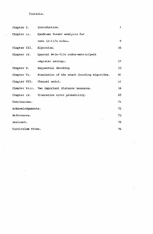
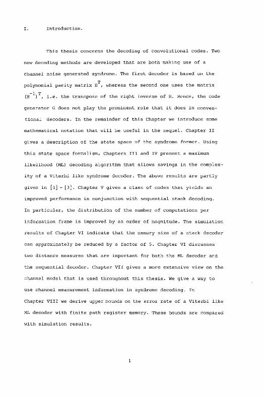

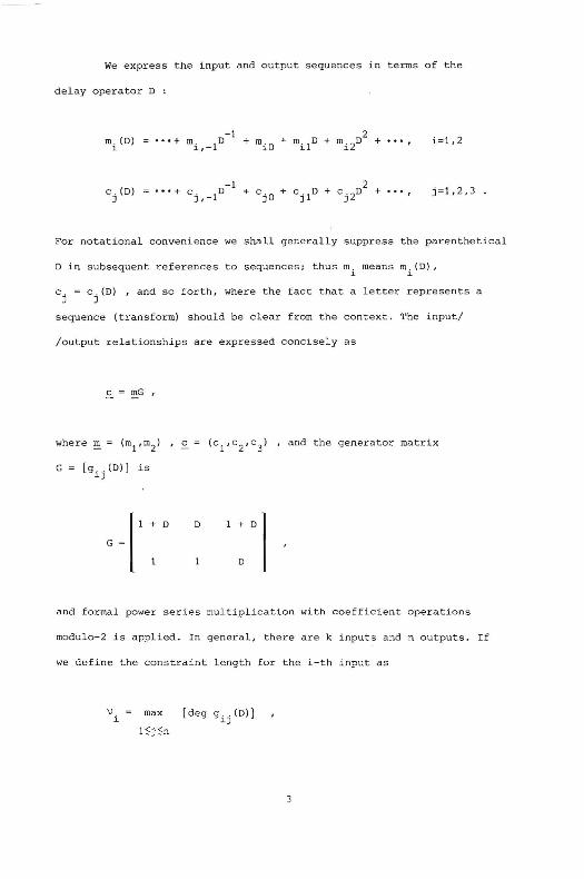
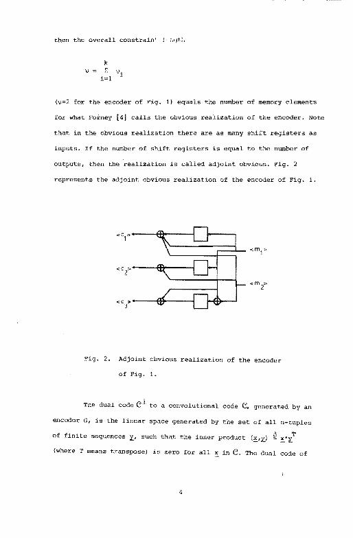
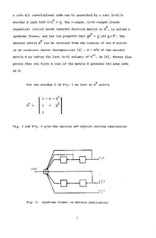
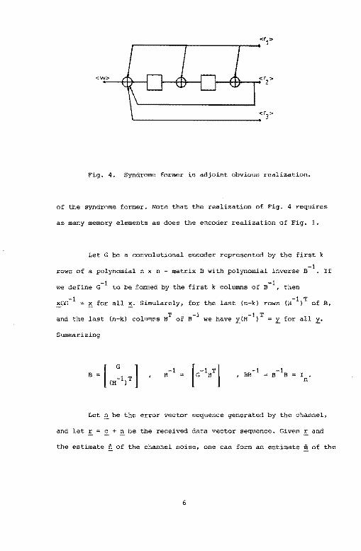
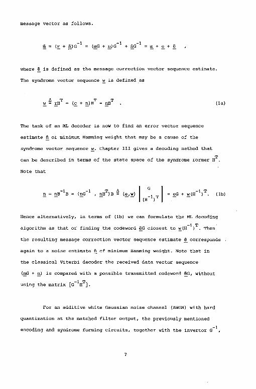
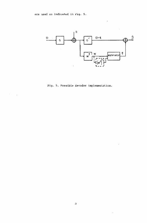
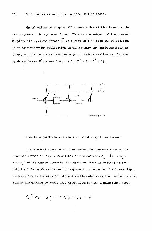
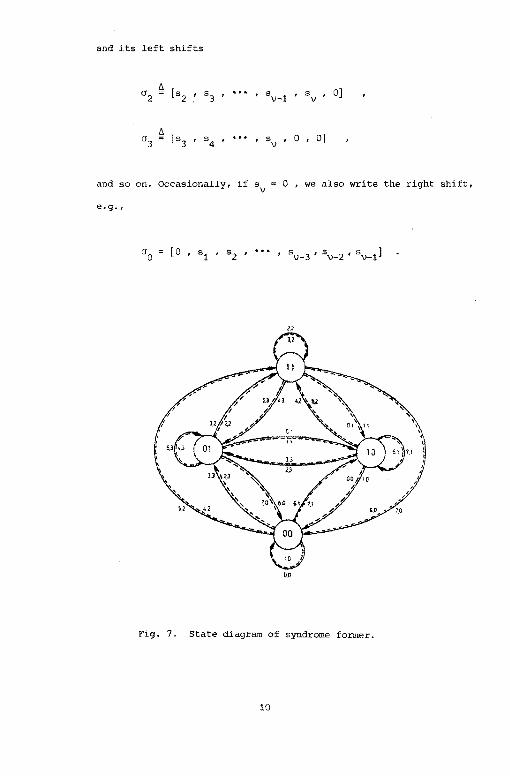
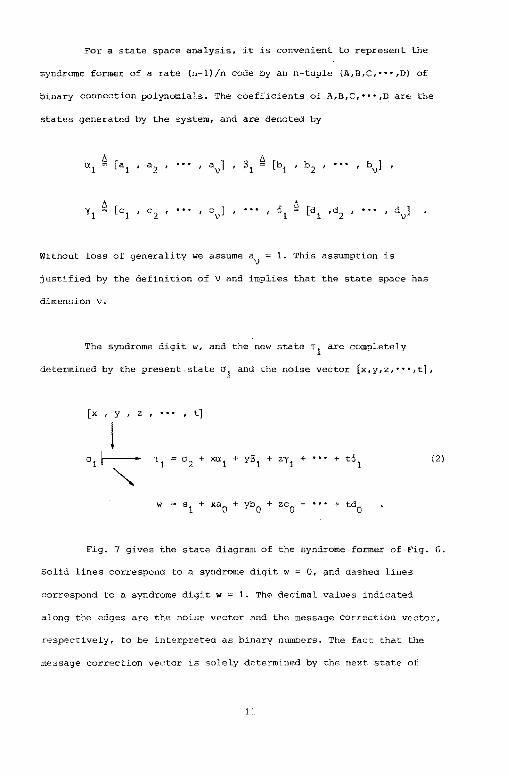

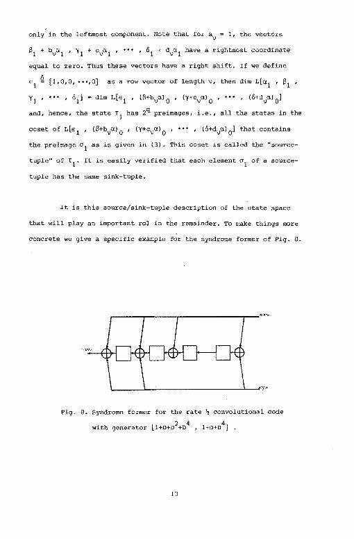
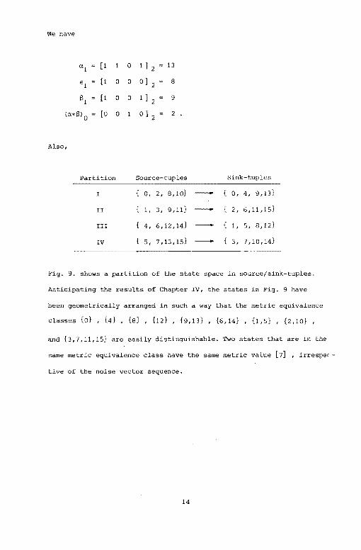

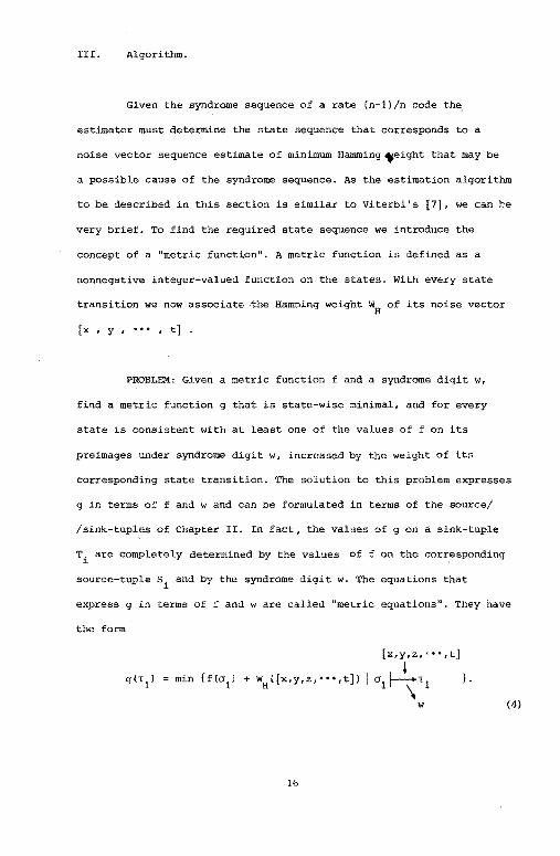
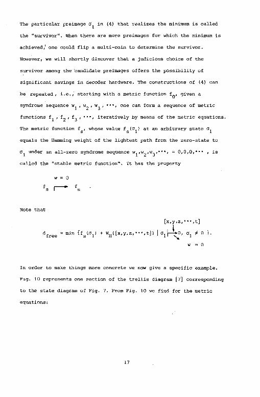
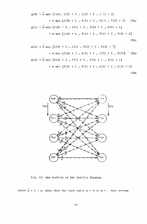
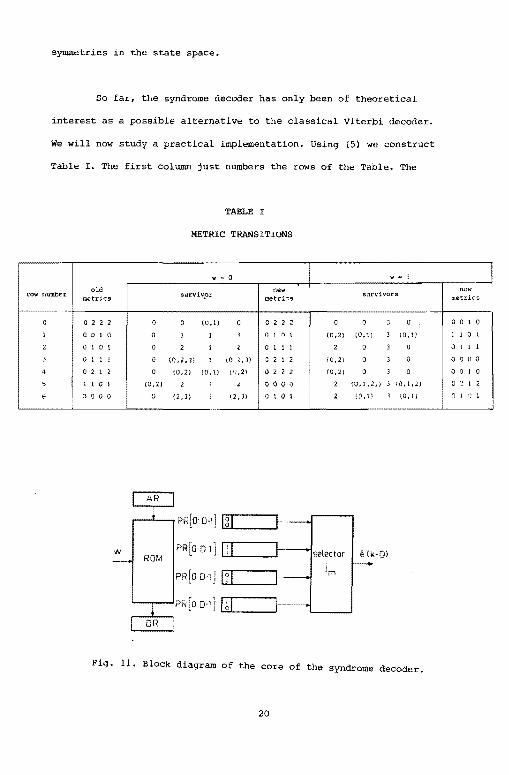
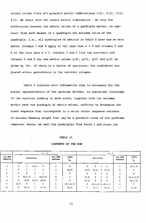
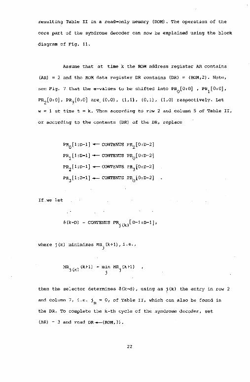
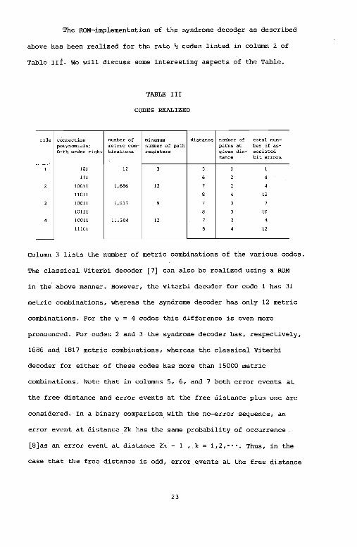
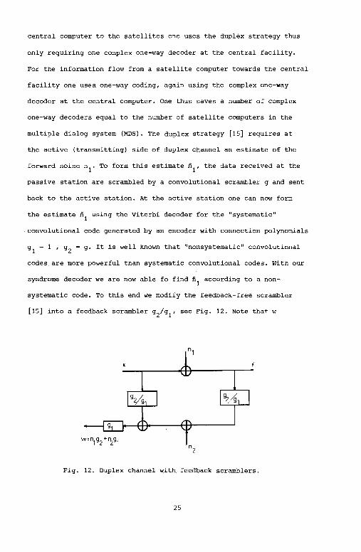
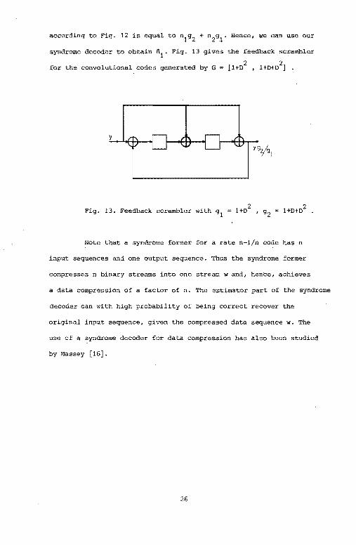
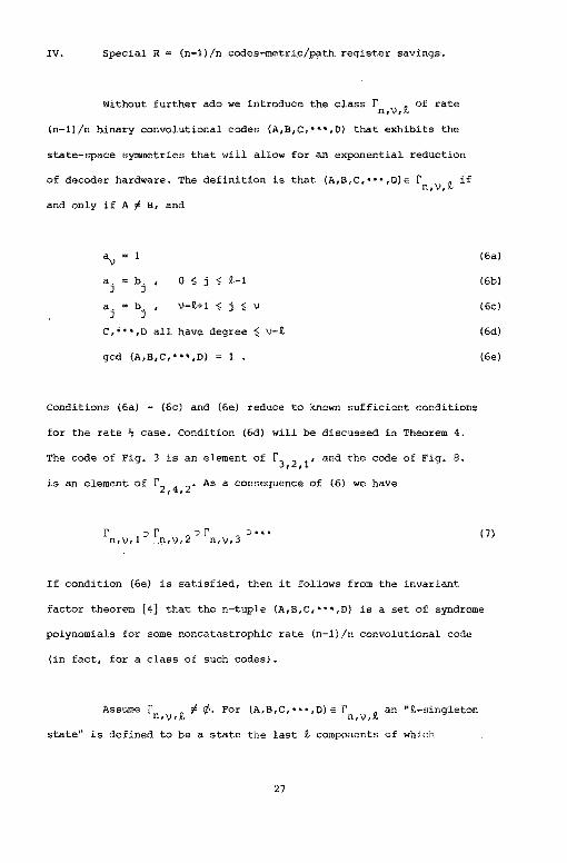

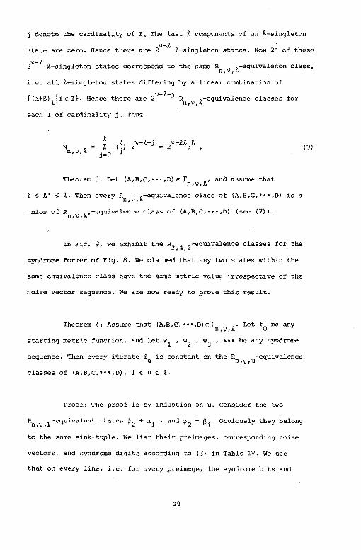
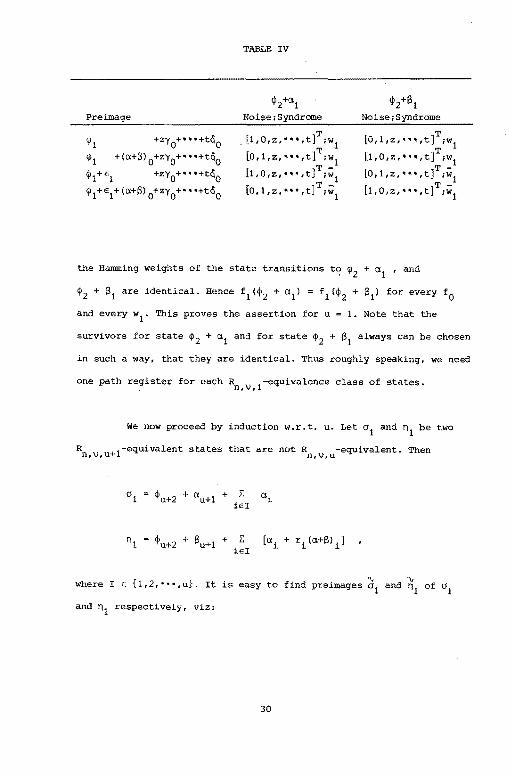
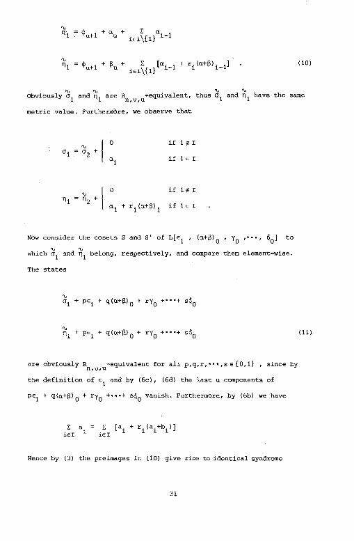
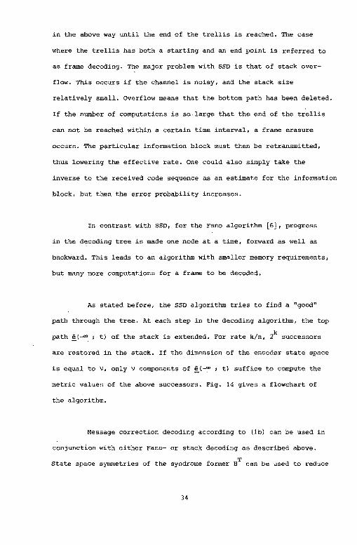
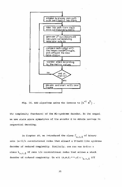
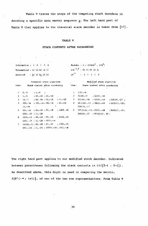

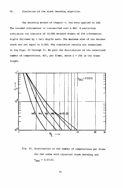
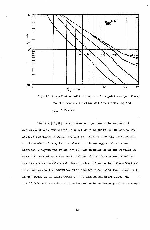
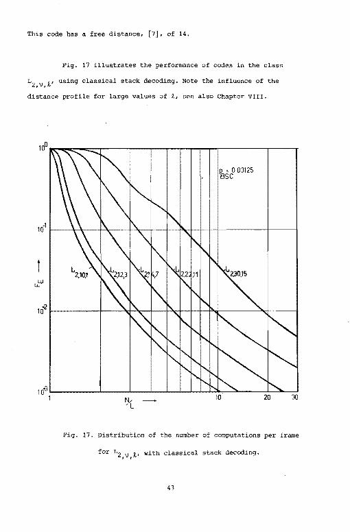
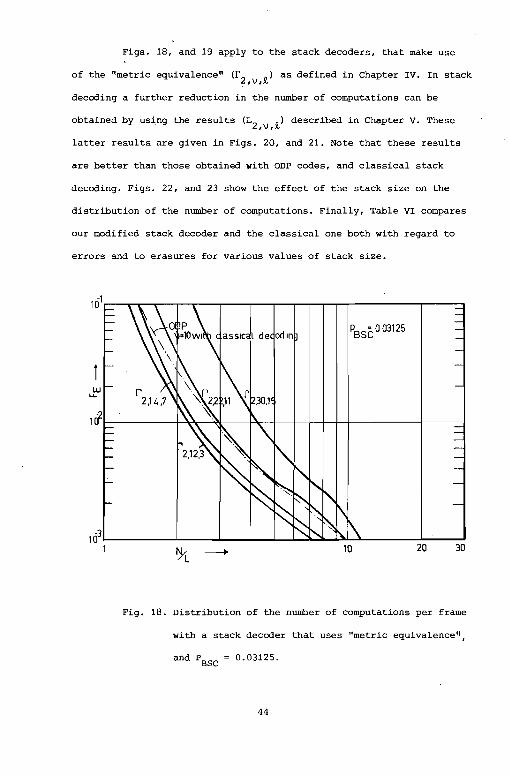
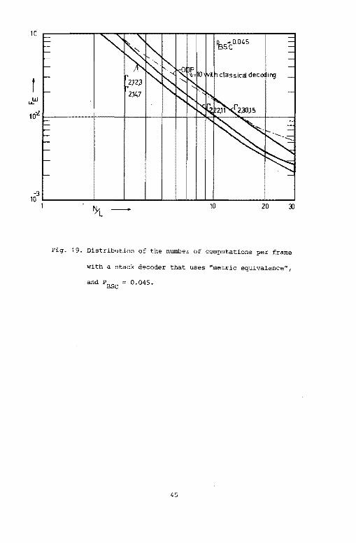
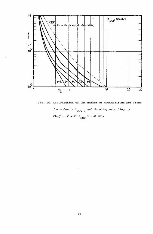
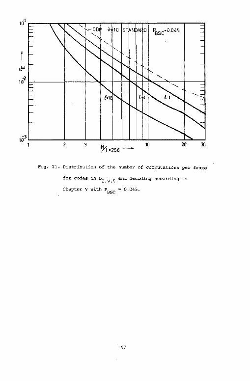
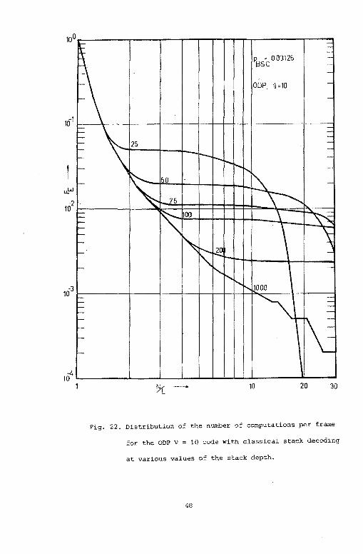
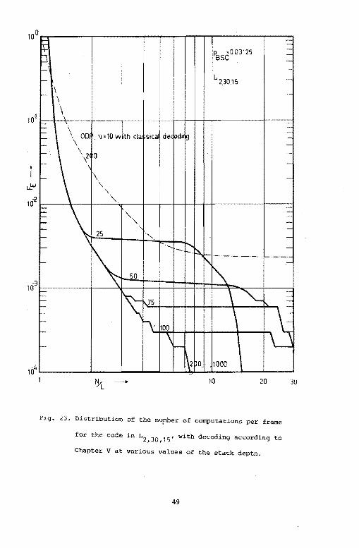
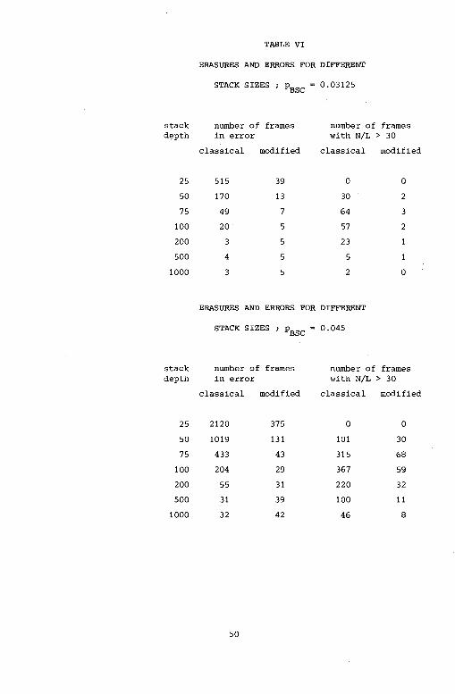
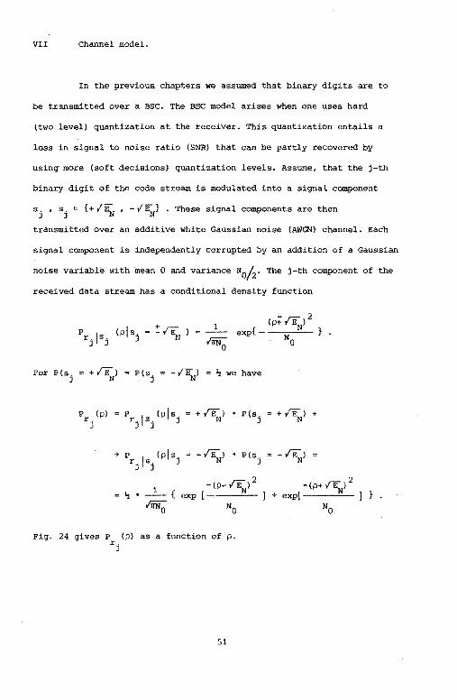
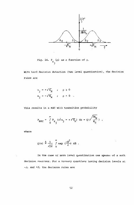
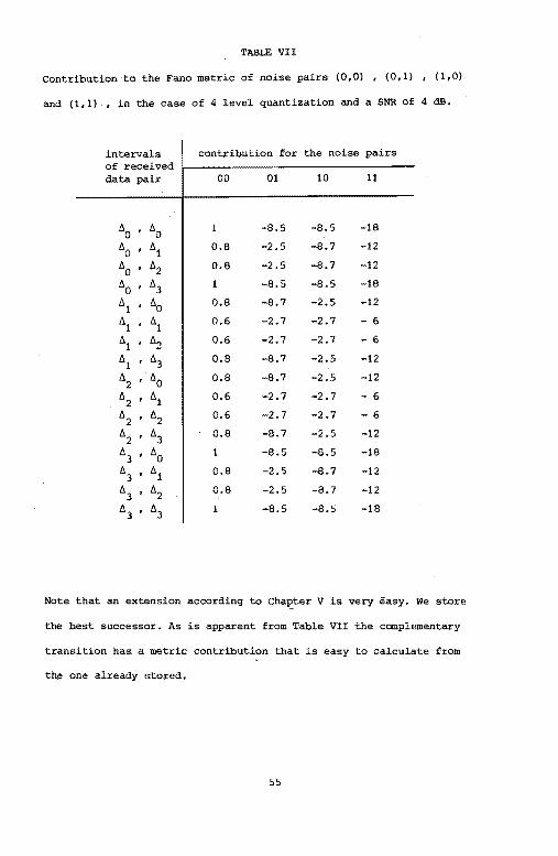
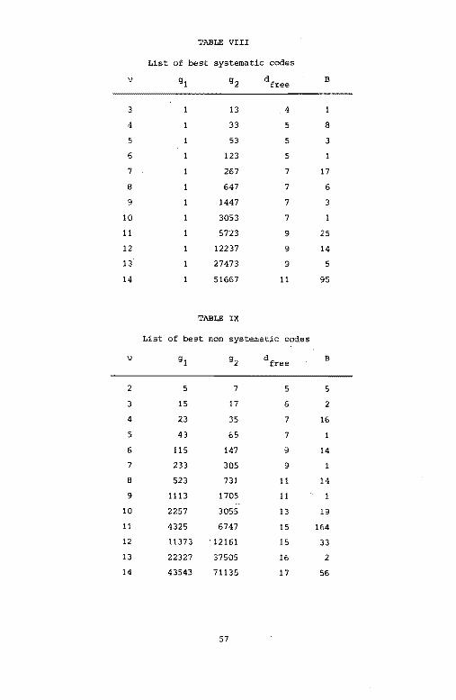
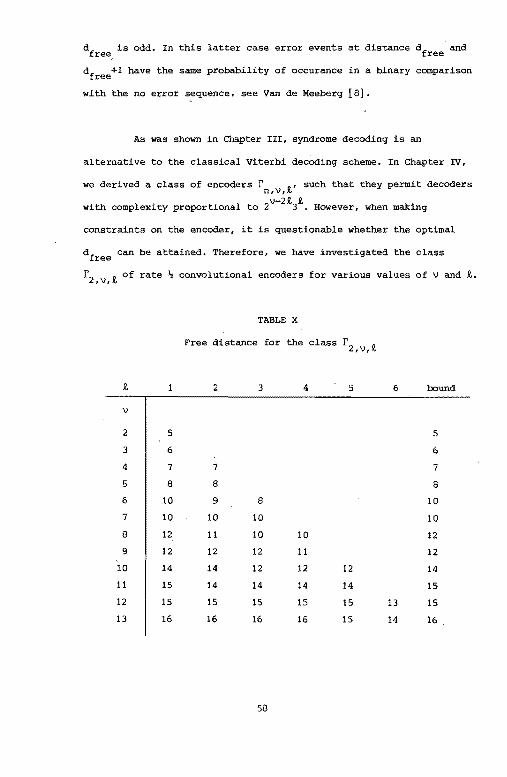
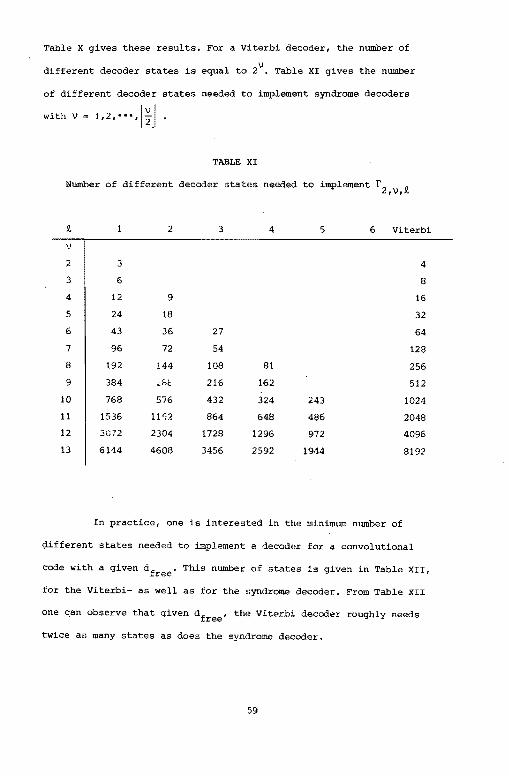
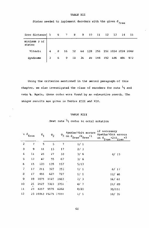
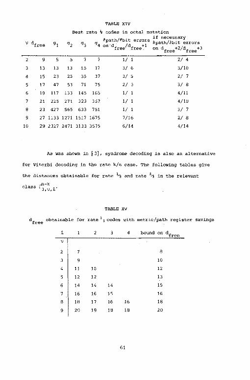
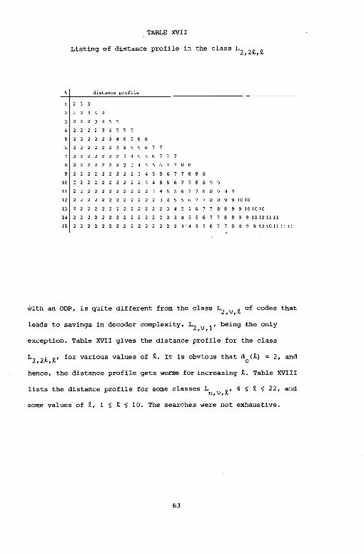
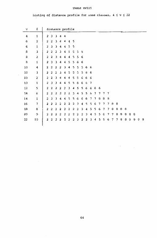
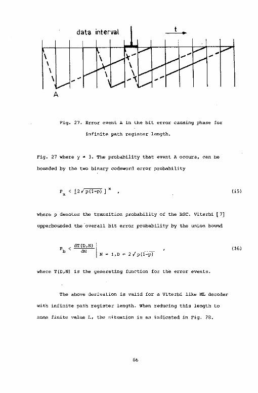
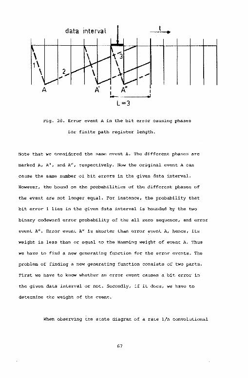
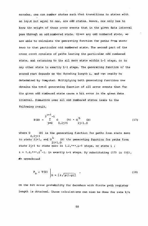
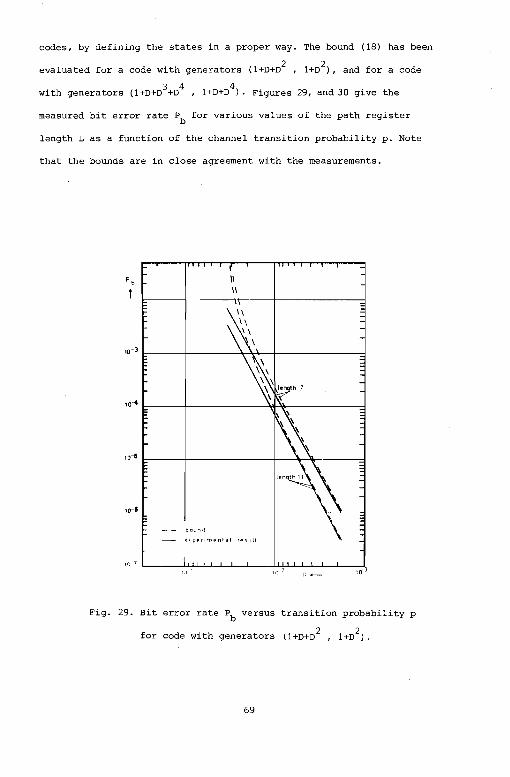
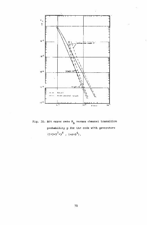


![Convolutional Codes. p2. OUTLINE [1] Shift registers and polynomials [2] Encoding convolutional codes [3] Decoding convolutional codes [4] Truncated.](https://static.documents.pub/doc/80x56/56649ec95503460f94bd6446/convolutional-codes-p2-outline-1-shift-registers-and-polynomials-.jpg)


