SYNTHESIS AND CHARACTERISATION OF MATERIALS WITH POTENTIAL MULTIFERROIC BEHAVIOUR by RHYS D’SOUZA A thesis submitted to The University of Birmingham for the degree of Master of Research School of Chemistry The University of Birmingham September 2008
Transcript
SYNTHESIS AND CHARACTERISATION OF MATERIALS
WITH POTENTIAL MULTIFERROIC BEHAVIOUR
by
RHYS D’SOUZA
A thesis submitted to
The University of Birmingham
for the degree ofMaster of Research
School of Chemistry
The University of Birmingham
September 2008
University of Birmingham Research Archive
e-theses repository This unpublished thesis/dissertation is copyright of the author and/or third parties. The intellectual property rights of the author or third parties in respect of this work are as defined by The Copyright Designs and Patents Act 1988 or as modified by any successor legislation. Any use made of information contained in this thesis/dissertation must be in accordance with that legislation and must be properly acknowledged. Further distribution or reproduction in any format is prohibited without the permission of the copyright holder.
Acknowledgements
I would like to thank my supervisor, Professor Greaves for his indispensable
advice and help during this project. When I started my project I did not know how to
use all the laboratory facilities that were necessary for my project. Therefore, I would
also like to take this opportunity to thank Jenny Readman for showing me how to use
the D5000 and Fiona Coomer for helping me to take magnetic measurements on the
PPMS and the SQUID. Special thanks goes to Ryan Bayliss for risking life and limb
when operating the high pressure oxygen furnace. The friendly atmosphere on level 5
has made my work really enjoyable.
i
Abstract
The ceramic method has been used to produce Aurivillius1 phase materials,
Bi3NbTiO9 and Bi4Ti3O12. The structures have been refined in A21am and Fmmm symmetry,
respectively. In addition, the fractional co-ordinates of the constituent atoms of these materials
has been calculated by Rietveld refinement.
A range of materials of general formula Bi5Fe1+xTi3-xO15 was produced with a value of
x ranging from 0 to 2.5, which is higher than has been previously been reported. Attempts to
produce Bi5Fe4O15, with all the Ti4+ sites occupied by iron atoms proved unsuccessful. The
space group of Bi5FeTi3O15 was determined to be A21am, however, the other 4-layer bismuth
phases proved to difficult to characterise without more data.
Increasing the number of pseudo-perovskite layers from 2 to 3 to 4 (from Bi3NbTiO9
to Bi4Ti3O12 to Bi5FeTi3O15 respectively) had a notable effect in increasing the size of the unit
cell along the z-axis, going from c=25.192(1)Å to c=32.785(1)Å to c = 41.179(1)
The magnetic properties of Bi5FeTi3O15, Bi5Fe2Ti2O15 and Bi5Fe3TiO15 have been
recorded, as part of an attempt to find multiferroic materials. The information collected would
suggest that Bi5FeTi3O15 and Bi5Fe3TiO15 display some degree of anti-ferromagnetic
behaviour, whereas Bi5Fe2Ti2O15 appears to be a paramagnet.
Failure to produce Bi5MnTi3O15 , using methods outlined by other researchers2,3, raises
doubts about the viability of manganese substitution into the bismuth-layer structure.
3.3.4.1 Magnetic Characterisation of Bi5Fe2Ti2O15 and Bi5Fe3TiO15 45
3.3.5 Attempted Synthesis of Bi5Fe4O15 47
3.4 Attempted Synthesis and Characterisation of Bi5Mn1+xTi3-xO15 48
4. Conclusions and Further Work 51
4.1 Conclusions 51
4.2 Further Work 52
5. References 54
Appendix A: X-ray Powder Diffraction Patterns
Appendix B: Mössbauer Spectroscopy
iv
Section 1: Introduction
1.1 Multiferroics
This project reports the study of a series of layered bismuth compounds, with
structures related to Aurivillius phases1 The main aim of this project was to achieve
significant substitution of magnetic ions into the aforementioned Aurivillius phases,
which will hopefully then have the potential to display multiferroic properties.
Multiferroic materials are commonly defined as those which simultaneously
display the properties of ferroelectricity and some form of magnetic ordering, either
ferromagnetism or anti-ferromagnetism. Some have included ferroelasticity as one of
the properties of multiferroic materials, however this property is not included in this
study.
Ferroelastic, ferroelectric and ferromagnetic properties can all have their
behaviour described by a phenomenon known as hysteresis. In fact, the reason that the
ferro- prefix is common for all three of these separate properties has its roots in the
fact that all properties share hysteresis behaviour. A hysteresis loop shows how two
parameters are related, such as the relationship between strain and mechanical stress
displayed by ferroelastic materials. Hysteresis behaviour can be described graphically
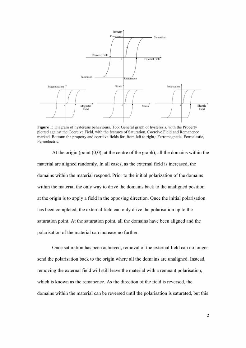
(Figure 1).
1
At the origin (point (0,0), at the centre of the graph), all the domains within the
material are aligned randomly. In all cases, as the external field is increased, the
domains within the material respond. Prior to the initial polarization of the domains
within the material the only way to drive the domains back to the unaligned position
at the origin is to apply a field in the opposing direction. Once the initial polarisation
has been completed, the external field can only drive the polarisation up to the
saturation point. At the saturation point, all the domains have been aligned and the
polarisation of the material can increase no further.
Once saturation has been achieved, removal of the external field can no longer
send the polarisation back to the origin where all the domains are unaligned. Instead,
removing the external field will still leave the material with a remnant polarisation,
which is known as the remanence. As the direction of the field is reversed, the
domains within the material can be reversed until the polarisation is saturated, but this
2
Figure 1: Diagram of hysteresis behaviours. Top: General graph of hysteresis, with the Property plotted against the Coercive Field, with the features of Saturation, Coercive Field and Remanence marked. Bottom: the property and coercive fields for, from left to right,: Ferromagnetic, Ferroelastic, Ferroelectric.
time saturation is achieved in the negative direction. The coercitivity of the material
relates to the coercive field, that is, the magnitude of the field that is required to
negate the behaviour induced in the material, after saturation.
If the external field is cycled between the positive and negative directions,
with a sufficiently powerful field, the polarisation of the material will rotate around
the hysteresis loop in an anti-clockwise direction. The area of the hysteresis loop is
proportional to the energy absorbed for each cycle of the hysteresis loop.
Smaller hysteresis loops are described as 'soft', where the polarisation of the
material can be switched comparatively easily. Soft hysteresis finds uses in
applications where the alignment has to be changed quickly, for instance transistors
use soft ferromagnets. Hysteresis loops described as 'hard' have much larger loops and
consequently altering the polarisation of these materials requires a greater amount of
energy. Hard hysteresis is useful for applications where a material has to be able to
retain its alignment for a significant amount of time. Obviously, not all materials
display either hard or soft hysteresis, and there are plenty of uses for materials that
display neither hard nor soft hysteresis.
Ferroelasticity is the property of displaying a spontaneous strain when stress is
applied. The property of ferroelasticity was first recognised in 19692. A ferroelastic
crystal is able to adopt two or more stable orientation states, specifically in the
absence of any mechanical stress or electric field. A ferroelastic material also has the
ability to convert between these multiple orientation states whenever mechanical
stress is applied3.
3
The property of ferroelectricity refers to a spontaneous polarization that can be
altered by an applied electrical field. Ferroelectricity occurs when cations are
displaced from their ideal sites in the unit cell, creating domains of dipoles which can
then be manipulated by an electric field.
When an electric field, E, is applied there is polarisation, P, which aligns the
domains in the ferroelectric material. More importantly, after the electrical
polarizations of many unit cells are aligned there exists a remanent polarization, so the
domains remain aligned, even when the electrical field is removed, which leads to
hysteresis behaviour.
The perovskite structure is typified by large A cations at the corners of the unit
cell with a smaller B cation at the centre of an
octahedron of oxygen anions in the middle of the unit
cell (Figure 2). In ferroelectric perovskites the central B
cation moves from its ideal position, giving rise to a
dipole moment. Ferroelectricity can exist in perovskite
and pseudo-perovskite structures due to ligand field
stabilization, as electron density from the oxygen 2p
state can be
donated to the formally vacant d-sub-shells of
the cation as it moves from its undistorted
position.
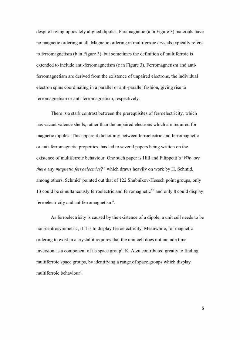
Ferrimagnetism (d in Figure 3) occurs in
situations where overall there is a net dipole,
4
Figure 2: An example of the perovskite unit cell (centred on B), with the blue spheres representing oxygen, black spheres representing the B cation and the white sphere representing the A cation.
Figure 3: Ordering of dipoles in magnetic materials. a) Paramagnetism, b) Ferromagnetism, c) Anti-ferromagnetism, d) Ferrimagnetism.
despite having oppositely aligned dipoles. Paramagnetic (a in Figure 3) materials have
no magnetic ordering at all. Magnetic ordering in multiferroic crystals typically refers
to ferromagnetism (b in Figure 3), but sometimes the definition of multiferroic is
extended to include anti-ferromagnetism (c in Figure 3). Ferromagnetism and anti-
ferromagnetism are derived from the existence of unpaired electrons, the individual
electron spins coordinating in a parallel or anti-parallel fashion, giving rise to
ferromagnetism or anti-ferromagnetism, respectively.
There is a stark contrast between the prerequisites of ferroelectricity, which
has vacant valence shells, rather than the unpaired electrons which are required for
magnetic dipoles. This apparent dichotomy between ferroelectric and ferromagnetic
or anti-ferromagnetic properties, has led to several papers being written on the
existence of multiferroic behaviour. One such paper is Hill and Filippetti’s ‘Why are
there any magnetic ferroelectrics?'4 which draws heavily on work by H. Schmid,
among others. Schmid5 pointed out that of 122 Shubnikov-Heesch point groups, only
13 could be simultaneously ferroelectric and ferromagnetic6,7 and only 8 could display
ferroelectricity and antiferromagnetism6.
As ferroelectricity is caused by the existence of a dipole, a unit cell needs to be
non-centrosymmetric, if it is to display ferroelectricity. Meanwhile, for magnetic
ordering to exist in a crystal it requires that the unit cell does not include time
inversion as a component of its space group8. K. Aizu contributed greatly to finding
multiferroic space groups, by identifying a range of space groups which display
multiferroic behaviour9.
5
The reason for the interest in multiferroic materials is due to their potential use
in commercial applications. The ability to utilise both magnetic and electric
polarisation opens many options in the field of data storage. For instance, using the
different hysteresis behaviours allows multiple memory state components, capable of
storing data in both the magnetic and the electric polarisations. Current memory
systems only allow data to be stored in either polarisation, but not both, depending on
the type of memory being used. Another possibility would be that multiferroic
materials would provide a pathway to non-volatile memory systems (NVRAM) that
would allow data to be stored, even in situations where the power supply is
interrupted10.
6
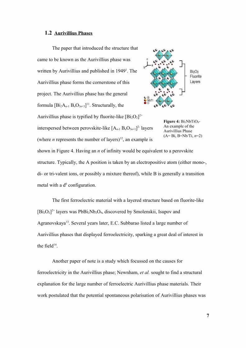
1.2 Aurivillius Phases
The paper that introduced the structure that
came to be known as the Aurivillius phase was
written by Aurivillius and published in 19491. The
Aurivillius phase forms the cornerstone of this
project. The Aurivillius phase has the general
formula [Bi2An-1 BnO3n+3]11. Structurally, the
Aurivillius phase is typified by fluorite-like [Bi2O2]2+
interspersed between perovskite-like [An-1 BnO3n+1]2- layers
(where n represents the number of layers)12, an example is
shown in Figure 4. Having an n of infinity would be equivalent to a perovskite
structure. Typically, the A position is taken by an electropositive atom (either mono-,
di- or tri-valent ions, or possibly a mixture thereof), while B is generally a transition
metal with a d0 configuration.
The first ferroelectric material with a layered structure based on fluorite-like
[Bi2O2]2+ layers was PbBi2Nb2O9, discovered by Smolenskii, Isupov and
Agranovskaya13. Several years later, E.C. Subbarao listed a large number of
Aurivillius phases that displayed ferroelectricity, sparking a great deal of interest in
the field14.
Another paper of note is a study which focussed on the causes for
ferroelectricity in the Aurivillius phase; Newnham, et al. sought to find a structural
explanation for the large number of ferroelectric Aurivillius phase materials. Their
work postulated that the potential spontaneous polarisation of Aurivillius phases was
7
Figure 4: Bi3NbTiO9- An example of the Aurivillius Phase(A= Bi, B=Nb/Ti, n=2)
largely due to the displacement of octahedral cations (B in the general structure) from
their ideal position at the centre of oxygen octohedra15.
While this work was influential in attempting to find a structural cause for the
high proportion of ferroelectric Aurivillius phases, it was superseded by a paper
suggesting a revised structure for Bi3NbTiO9. Thompson, et al., later reviewed the
structure and concluded that it was the displacement of Bi3+, rather than octahedral
cations that was the major contributing factor to ferroelectric behaviour16. Thompson,
et al. later showed that this was also true of other Aurivillius phase crystals,
challenging previous notions17. This theory is also supported by research into
multiferroic perovskite structures, such as BiMnO3, and BiFeO3, whose ferroelectric
behaviour is also the result of A cation displacement18.
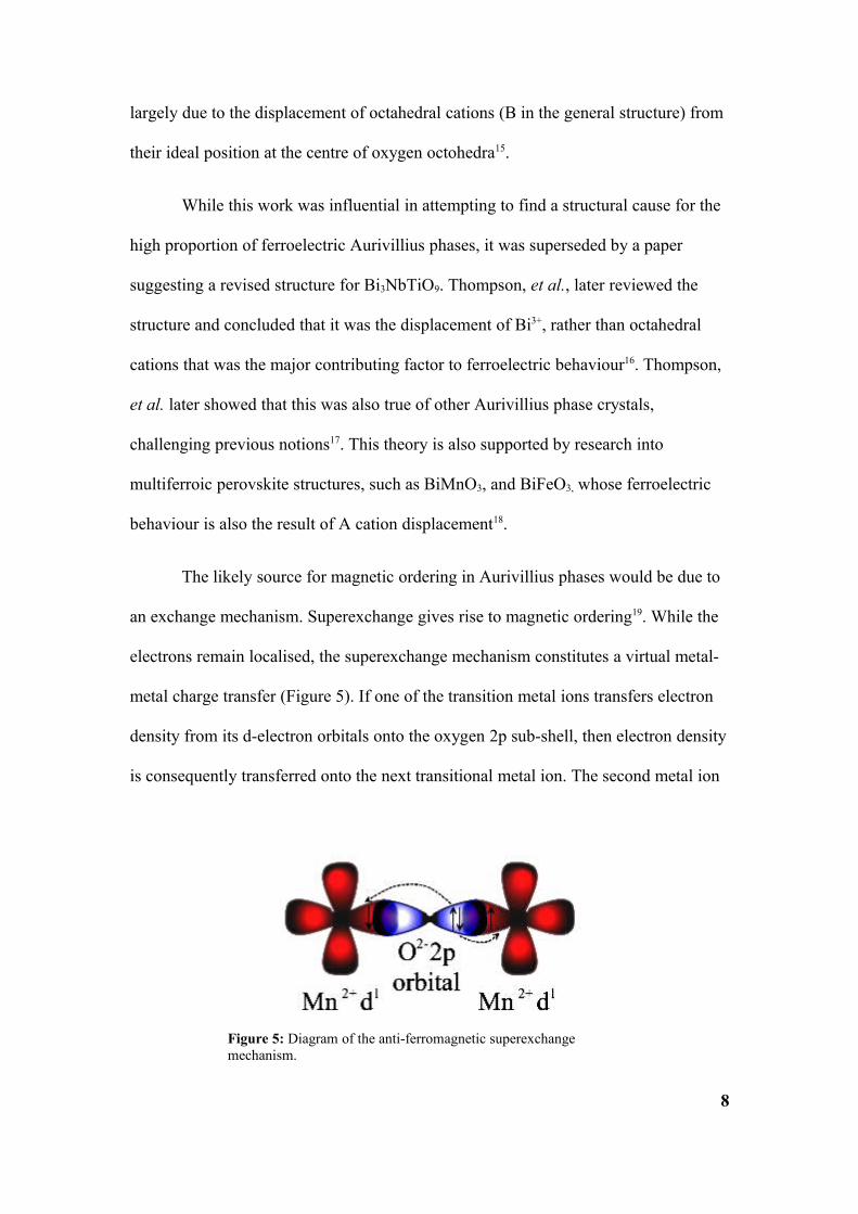
The likely source for magnetic ordering in Aurivillius phases would be due to
an exchange mechanism. Superexchange gives rise to magnetic ordering19. While the
electrons remain localised, the superexchange mechanism constitutes a virtual metal-
metal charge transfer (Figure 5). If one of the transition metal ions transfers electron
density from its d-electron orbitals onto the oxygen 2p sub-shell, then electron density
is consequently transferred onto the next transitional metal ion. The second metal ion
8
Figure 5: Diagram of the anti-ferromagnetic superexchange mechanism.
must have an opposite electron spin, otherwise superexchange cannot occur, as the
electron density cannot be transferred. As the transition metal ions have opposite spin,
this gives rise to anti-ferromagnetic ordering.
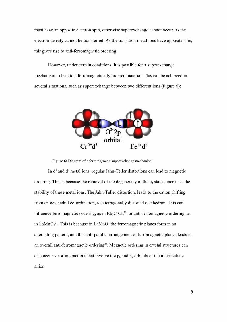
However, under certain conditions, it is possible for a superexchange
mechanism to lead to a ferromagnetically ordered material. This can be achieved in
several situations, such as superexchange between two different ions (Figure 6):
In d4 and d9 metal ions, regular Jahn-Teller distortions can lead to magnetic
ordering. This is because the removal of the degeneracy of the eg states, increases the
stability of these metal ions. The Jahn-Teller distortion, leads to the cation shifting
from an octahedral co-ordination, to a tetragonally distorted octahedron. This can
influence ferromagnetic ordering, as in Rb2CrCl420, or anti-ferromagnetic ordering, as
in LaMnO321. This is because in LaMnO3 the ferromagnetic planes form in an
alternating pattern, and this anti-parallel arrangement of ferromagnetic planes leads to
an overall anti-ferromagnetic ordering22. Magnetic ordering in crystal structures can
also occur via π-interactions that involve the px and py orbitals of the intermediate
anion.
9
Figure 6: Diagram of a ferromagnetic superexchange mechanism.
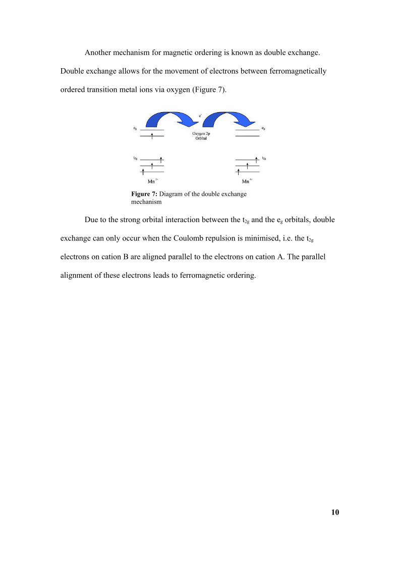
Another mechanism for magnetic ordering is known as double exchange.
Double exchange allows for the movement of electrons between ferromagnetically
ordered transition metal ions via oxygen (Figure 7).
Due to the strong orbital interaction between the t2g and the eg orbitals, double
exchange can only occur when the Coulomb repulsion is minimised, i.e. the t2g
electrons on cation B are aligned parallel to the electrons on cation A. The parallel
alignment of these electrons leads to ferromagnetic ordering.
10
Figure 7: Diagram of the double exchange mechanism
1.3 B-Cation Doping in Bismuth Titanates
In bismuth titanate, Bi4Ti3O12, the Bi3+ cation has been replaced, at least to
some extent, by a variety of lanthanoids, including La3+, Pr3+, Nd3+, Sm3+, Eu3+,
Gd3+, Tb3+, Dy3+, Ho3+, Er3+, Tm3+, Yb3+, Lu3+. As the radius of the dopant
decreases, the amount by which it can substitute for Bi3+ also decreases.
As well as lanthanoids, alkali metals, Na+, K+, Li+, have been used as dopants
for bismuth ions to induce piezoelectric behaviour in Aurivillius phase materials. The
piezoelectric behaviour of the alkali metal substituted materials can be further
improved by doping with cerium oxide23.
Substituting a metal cation for Ti4+ in the bismuth titanate structure requires
certain criteria to be met. The first consideration is the balancing of electronic
charges. Although only ions with a 4+ charge can be switched on a like-for-like basis,
by mixing dopants, it is possible to use cations with various oxidation states. For
instance, doping may involve a mixture of 3+ and 5+ ions, or a variety of A cation
substitutions to balance the charges involved.
The second consideration for substitution is the size of the ionic radius. The
tolerance factor ( t=r a1.40
2 rb1.40 ) of the pseudo-perovskite layer is a smaller
range than that of a standard perovskite (0.81-0.93 as opposed to 0.77-1.0124). This
means that the ionic radius of the octahedral cation must be within a range of
0.58-0.65Å. The lower limit of this range is caused by the loss of stability of the
pseudo-perovskite structure, due to the internal strain induced when attempting to fit
11
smaller cations. Meanwhile, the upper limit is a result of the potential mismatch in
size between the (Am-1BmO3m+1) pseudo-perovskite and (Bi2O2)2+ layers; if the
layers cannot align then a stable structure cannot be formed25.
This factor is seen in the cases of Ge4+, whose ionic radius of 0.54 Å is outside
the range that can be substituted, as it is too small. Other examples include Sn4+, Hf4+
and Zr4+, whose radii of 0.69Å, 0.71Å and 0.72Å respectively, put them outside the
appropriate range, but this time at the opposite end of the scale, being too large for
substitution.
An alternative to A site or B site cation substitution would be double
substitution. Examples of double substitution, where both the bismuth and titanium
cations are substituted, include the substitution of Ca2+, Sr2+, Ba2+ and Pb2+ for
bismuth, with a complementary substitution of titanium for either niobium or tantalum
to balance the charges involved.
The relationship between ionic radius and lattice a parameter for the layer has
been observed to be a= 0.6rA + 1.33rB + 2.36Å. Ideally, the parameter, a, is as close
to the lattice parameter of the Bi2O2 layer (3.80Å) as possible. Any a calculated to be
over 4Å causes enough internal strain to destabilise the structure25. From the
coefficients, it is quite clear that the size of the B site cation is a more significant
factor in regards to stability than the A site cation.
Therefore, Co3+ (0.61Å), Cr3+ (0.615Å), Fe3+ (0.645Å), Fe4+ (0.585Å) and
Mn3+ (0.645Å) have potential for substantial substitution. Compounds that have been
12
synthesised include Bi4Ti(3-2x)NbxFexO12 (x= 0.25, 0.5)26 and Bi4Ti(3-x)MnxO12 (x=
0.05, 0.1, 0.2)27.
Another possibility is to combine Bi4Ti3O12 and relatively easy to form
Bi5Ti3BO15 (where B= Mn, Fe, Cr, etc.) through
perovskite layer intergrowth, where the perovskite layer
alternates between the two Aurivillius phases.
In this way, two Aurivillius phases can be
combined to make a larger layered structure, as long as
the constituent phases differ in size by only one layer,
e.g. (Bi2O2)(Am-1BmO3m+1) + (Bi2O2)(A’mB’m+1O3m+4) =
Bi4A2m-1B2m+1O6m+928.This intergrowth method has been
used to create Bi9Ti6CrO27, amongst others29. With
careful planning it is possible to use intergrowth
structures (Figure 8), to improve the properties of existing Aurivillius phase materials
by creating stronger hysteresis30.
13
Figure 8: Diagram of an intergrowth structure.
1.4 Aims of this Project
This thesis will focus on several key areas:
● The attempt to form and characterise Bi3TiNbO9.
● The attempt to form and characterise Bi4Ti3O12.
● The attempted synthesis and characterisation of Bi5Fe1+xTi3-xO15 compounds.
These compounds feature higher Fe content than has previously been reported.
The characterisation of these materials also includes the magnetic
characterisation, to indicate possible multiferroic behaviour.
● An attempt to synthesise Bi5Mn1+xTi3-xO15 using similar methods to the
production of Bi5Fe1+xTi3-xO15 compounds.
14
Section 2: Experimental
2.1 Preparation Techniques
The means by which all samples were prepared is known as the ceramic
method. The ceramic method involves the grinding of stoichiometric quantities of
powders to form a homogeneous mixture. Although grinding can be done by
mechanical means, the grinding used in this thesis was done by hand, using a mortar
and pestle. The various reagents used were all 99.999% oxide powders from Sigma-
Aldrich.
The homogeneous mixture was then heated in a furnace. Typically, several
different heating stages using different temperatures, heating rates, and durations were
used to achieve the desired effect. In between heat treatments the mixture was ground
again to refresh the reaction interfaces between the various powders. This ensures the
best rate of reaction, as it improves the surface area and mobility of the reagents.
Reaction conditions were altered by using oxygen and 10% hydrogen/90%
nitrogen gas when appropriate. The Bi5Fe1.5Ti2.5O15 and Bi5Fe2Ti2O15 were both treated
using a high oxygen pressure furnace. In the high oxygen pressure furnace, oxygen is
supplied to a regulator at 220 bars of pressure. The oxygen is then pumped into the
furnace, creating a much higher overall pressure, due to the higher temperature.
Using the combined gas law the pressure inside the furnace can be
calculated. The combined gas law, is itself, an amalgam derived of Boyle’s Law,
Charles’s Law and Guy-Lussac’s Law. Each of these thermodynamic laws
demonstrates how one variable is affected by change in the other. For instance,
Boyle’s Law shows the relationship between pressure and volume, Charles’s Law
15
shows the relationship between volume and temperature and Gay-Lussac’s Law
demonstrates how pressure and temperature are related. The combined gas law is:
P1 V 1
T 1=
P2V 2
T 2
As the volume of the furnace chamber remains constant, i.e. V1=V2, so this variable
can be removed from both sides of the equation. This gives us:
P1
T 1=
P2
T 2
The initial pressure, P1, is 220 bar, the initial temperature, T1, is room temperature at
298 K. The temperature inside the furnace increases to 1123 K, increasing the furnace
pressure to 829 bar.
2.1.1 Preparation of Bi 3NbTiO9
To prepare Bi3NbTiO9, stoichiometric amounts of Bi2O3, Nb2O5 and TiO2 were
ground together, for 30 minutes in a mortar and pestle, before being placed in a
furnace. The homogeneous ground mixture was then fired in a Carbolite CWF 1300
furnace at 1160°C for 10 hours. This temperature was chosen due to work performed
showing the relationship between sintering temperature and percentage yield31.
2.1.2 Preparation of Bi 4Ti3O12
Bismuth titanate was prepared in a similar manner to Bi3NbTiO9, but without
Nb2O5 as a reagent. In addition, for bismuth titanate the stoichiometric amounts of
Bi2O3 and TiO2 in the furnace were only heated to 1000°C for 10 hours, the same
duration as the synthesis of Bi3NbTiO9.
16
2.1.3 Preparation of Bi 5Fe1+xTi3-xO15
The majority of the various samples of Bi5Fe1+xTi3-xO15 (with x ranging from 0
to 1 and increasing in increments of 0.1) were prepared with two separate firings of
stoichiometric amounts of Bi2O3, Fe2O3 and TiO2. The two firings took place at 850°C
in oxygen at atmospheric pressure, with the first firing lasting for 10 hours, then the
second lasting for 8 hours.
The exceptions to this method are Bi5FeTi3O15, Bi5Fe1.1Ti2.9O15 and
Bi5Fe1.6Ti2.4O15. The sample of Bi5FeTi3O15 was formed by a single 12 hour firing at
1050°C in air. The sample of Bi5Fe1.1Ti2.9O15 was formed by a 12 hour firing at
1050°C in air, followed by two firings in oxygen at atmospheric pressure at 850°C,
first for 10 hours and then for 8 hours. To prepare Bi5Fe1.6Ti2.4O15, following two
separate firings at 850°C in oxygen at atmospheric pressure, first for 10 hours, then
for 8 hours; it was found that an initial 8 hour firing under the same reaction
conditions was necessary.
2.1.4 Preparation of Bi 5Fe2.5Ti1.5O15 and Bi5Fe3TiO15
For these samples, stoichiometric amounts of Bi2O3, Fe2O3 and TiO2 were
used. The pre-sintering was carried out at 800°C for 12 hours, while sintering was
carried out at 850°C for 12 hours. A fifteen minute period of grinding with a mortar
and pestle took place between the pre-sintering and sintering phases. It is important to
note that both the heat treatments took place in air, rather than in oxygen (as was used
previously) therefore, for future reference, those materials may not require an
atmosphere of oxygen when being fired, although this is unknown without any further
evidence.
17
2.2 Characterisation Techniques
2.2.1 X-ray Diffraction and Rietveld Refinement
2.2.1.1 X-ray Diffraction
The primary method used for determining the size and symmetry of unit cells
is X-ray diffraction. Crystalline structures are comprised of many unit cells, a unit cell
being the smallest arrangement of atoms that can be used to recreate the crystal purely
by translational displacements. As the atoms form repeating units in space, it can be
related to a space lattice of points, known as a Bravais lattice. In three dimensions,
there are a total of fourteen distinct Bravais lattices32.
Due to the periodicity of the repeating unit cells, there are repeating planes
made up of atoms, whose electron density has the effect of scattering X-rays. A
crystal lattice will have many sets of planes, each with their own interplanar spacing.
These sets of planes act as a diffraction grating for X-rays of the appropriate
wavelength.
A plane is defined by its Miller indices, a set of three values, (hkl), which give
the reciprocal lattice vector that lies perpendicular to the plane in question. Each plane
has a unique reciprocal lattice vector, so an individual unit cell can be determined by
its Miller indices.
If we consider two parallel planes inside a crystal, which are both incident to
two monochromatic X-rays (as seen in Figure 9); the path difference for wave b, as
opposed to wave a, has to be equal to an integer number of wavelengths (nλ) for it to
lead to constructive interference. The path difference between a and b is equal to 2l.
18
As d is the hypotenuse of a right-angled triangle made by the perpendicular to the
plane and the vectors of waves a and b, l is closely related to d, the distance between
the planes, given by the equation:
l=d sin
From this information, Bragg's law can be calculated, which is used to
interpret the XRD data:
2 d sin =n
Where
d = Distance between planes (Å)
θ = Angle of refection
n = Order of Diffraction (an
integer, which can be controlled
for calculation purposes)
λ = Wavelength of source
(1.5406Å)
As the value of λ is known, n is set to 1 and the θ values are the data collected
by XRD, it is possible to calculate the d-spacing. This in turn, allows the
determination of the unit cell parameters, symmetry, atomic positions and unit cell
size.
The intensity of the reflection depends on a variety of different factors and is
given by:
I hkl=m F hkl2 ALp
19
Figure 9: Diagram showing the interaction between two X-rays (waves a and b) and two parallel planes, separated by distance d, to demonstrate Bragg's Law
Where m represents the multiplicity of the unit cell, Fhkl is the structure factor, A
represents absorption and Lp is the Lorentzian polarisation factor. Absorption
increases for heavier atoms. The structure factor, Fhkl, takes into account the resultant
effect of wave scattering by all the atoms in the unit cell, in the (hkl) direction. It is
given by the following equation for n atoms in a unit cell:
F hkl=∑1
n
f n exp[2 i hxnkynlzn]exp[−Bnsin 22 ]
The factor fn refers to the scattering factor, a measure of how effectively an
atom scatters X-rays, largely based on the number of electrons the atom contains. The
position of the atom is given by its coordinates, xn, yn, zn. The Debye-Waller
temperature factor has the symbol Bn, which is related to the displacement of an atom.
Bn=82 U
Where U is the mean square amplitude of atom vibration, which is given in Å2.
With all this information, X-ray diffraction is a powerful technique which can tell us a
great deal about the unit cell.
There are two different types of X-ray diffraction, X-ray powder diffraction
(XRPD) and single crystal diffraction. Single crystal data allows the user to accurately
determine each hkl reflection and its intensity. Analysis of these data allow the precise
determination of the space group and thus, its atomic positions and lattice parameters.
The major drawback however, is that single crystal data require the growth of a large
crystal, which in practise can be quite difficult.
X-ray powder diffraction, as the name suggests, allows the use of powders to
derive the structural information, which are easier to prepare as opposed to single
crystals. The XRPD data can be compared to a database containing a large number of
20
powder diffraction files, which allows for relatively easy identification of the different
phases that are present in the powder sample. The database contains data collated by
the International Centre for Diffraction Data33.
All XRPD data in this thesis are from a Siemens D5000 diffractometer using
Cu Kα1 radiation (λ = 1.5406Å) with a Ge primary beam monochromator and position
sensitive detector. The X-rays are generated by bombarding Cu with high energy
electrons. This causes the Cu to lose an electron from the K shell (1s orbital), creating
a vacancy. This partial vacancy of the K shell leads to the transition of an electron
from either the 2p or 3p shells. This transition leads to the emission of radiation in the
X-ray region of the electromagnetic spectrum.
For Cu, three intense X-ray wavelengths arise, namely Cu Kα1, Cu Kα2 and Cu
Kβ. The Cu Kβ wavelength is generated by the transition of electrons from the 3p
orbital, while the Cu Kα1 and Cu Kα2 wavelengths are generated by transition of
electrons from the 2p orbital, differentiated due to the different spin states of electrons
in the 2p subshell. The Ge monochromator removes the less intense Cu Kα2, Cu Kβ
and white X-rays, leaving the more intense Cu Kα1 radiation.
21
2.2.1.2 XRPD analysis and Rietveld Refinement
Initial analysis was carried out by comparing powder diffraction files in the
Diffracplus EVA database to the XRPD data collected from the powder samples.
Subsequently, Rietveld refinement was carried out using the GSAS suite of
programmes34. It is important to note that Rietveld refinement is precisely that, a
refinement technique; the starting point for determining the unit cell will come from
another source. In the case of this thesis, all starting unit cell information was taken
from appropriate published research found using the Inorganic Crystal Structure
Database (ICSD), which contains 89,064 inorganic structures35.
Heavy metals, such as bismuth, are very good at absorbing and scattering X-
rays, which leads to a change in intensity for certain peaks. Therefore, prior to
Rietveld refinement it is necessary to perform an absorption correction.
Rietveld refinement is a least-squares method of calculating and refining
lattice parameters, atom positions and thermal vibrations, which was developed by
H.M. Rietveld in 196732,36.
Rietveld refinement takes into account the intensity at each XRPD data point
and then uses a least-squares method to estimate the structural parameters. Rietveld
refinement allows for a more advanced analysis than an integration method, as it
allows for impurities and overlapping peaks caused by the same phase, which would
be difficult to separate through other means.
The strength of the least-squares method is that it is a method for solving
overdetermined systems. For powder diffraction the equations represent powder
profile points and the variables refer to parameters.
22
The least squares method is the minimization of the following equation:
M=∑ w y iobs−y icalc2
The variable w is the weighted mean and yi(obs) and yi(calc) are the observed and
calculated intensities for the ith point, respectively. Minimization of this equation
gives parameter estimates for the set of linear equations. The minimum for the
equation can be found by calculating where the first derivative of M is equal to 0, i.e.:
∑ w y iobs−y icalc 2y icalc
p j=0
Where δpj, represents a parameter shift. The downside of this method is that it
may lead to a false minima, that is, a solution for the above equation, but not the
optimal (and sometimes not even physically possible) solution for the equation.
The parameters which indicate whether a calculated pattern is a good fit to the
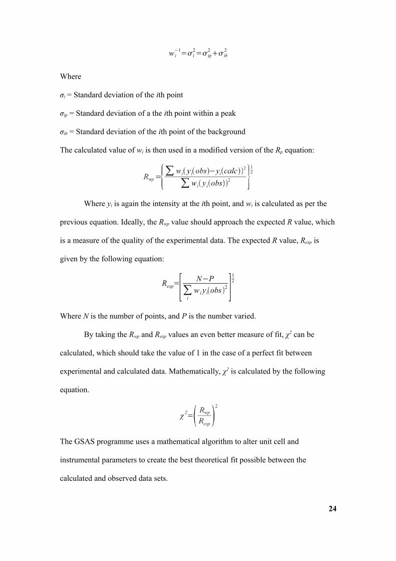
observed pattern are Rp, Rwp and χ2. The Rp value gives the difference between the
calculated and observed pattern with no bias given to any specific point, giving a
measure of how similar the two patterns are, in general. The equation used is:
R p=∑∣y iobs − y icalc∣
∑ y iobs
Where yi is the intensity for a given point i.
In a similar manner, Rwp gives a similar measure to Rp of the difference
between the observed and calculated values. However, Rp does not take into account
the standard deviation of peak heights and background radiation which makes Rwp a
more useful measure of similarity between the two data sets. Via the following
formula Rwp can be calculated:
23
w i−1=i
2=ip2 ib
2
Where
σi = Standard deviation of the ith point
σip = Standard deviation of a the ith point within a peak
σib = Standard deviation of the ith point of the background
The calculated value of wi is then used in a modified version of the Rp equation:
Where yi is again the intensity at the ith point, and wi is calculated as per the
previous equation. Ideally, the Rwp value should approach the expected R value, which
is a measure of the quality of the experimental data. The expected R value, Rexp is
given by the following equation:
Rexp=[ N−P∑
iw i y iobs 2 ]
12
Where N is the number of points, and P is the number varied.
By taking the Rwp and Rexp values an even better measure of fit, χ2 can be
calculated, which should take the value of 1 in the case of a perfect fit between
experimental and calculated data. Mathematically, χ2 is calculated by the following
equation.
The GSAS programme uses a mathematical algorithm to alter unit cell and
instrumental parameters to create the best theoretical fit possible between the
calculated and observed data sets.
24
A key danger when using GSAS is that the χ2 value can adopt a false
minimum. In this situation, the χ2 value sits in a 'well' of possible χ2 values and needs
to adopt a higher value than the false minimum to move to a superior fit. As the
algorithm seeks to find the lowest χ2 value, adopting a higher value is seen as sub-
optimal, even though it is necessary in the long-term.
25
2.2.2 Physical Properties Measurement System
Magnetic measurements were performed using a Quantum Design Model 6000
Physical Properties Measurement System (PPMS) using AC Susceptibility and DC
Magnetisation (ACMS) method. Measurements were carried out, both in zero-field
cooled (ZFC) and field-cooled (FC) conditions, using the DC extraction or induction
method. The AC magnetic susceptometer (ACMS) uses sensing coils to measure the
changes in magnetic flux that are caused by a magnetised sample.
The sample is inserted into a straw and lowered into position inside a pick-up
coil. The pick-up coil is designed to detect any flux changes as the magnetised sample
is moved through the coil37. The external magnetic field is applied by a niobium-
titanium alloy, which acts as a superconducting magnet. The ZFC measurement is
taken initially, after the sample is cooled to 3-4K, it is warmed without any external
magnetic field. Once warmed, the sample is then cooled in the presence of an external
field, which allows the FC measurements to be taken on warming. By calculating the
magnetic susceptibility of a material, its magnetic properties can be defined.
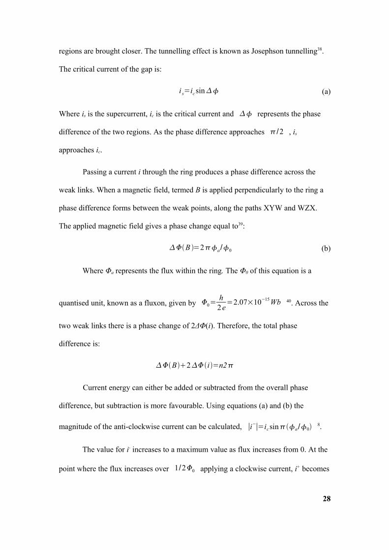
To measure magnetic interactions within a material a Superconducting
Quantum Interface Device (SQUID) is sometimes used. A SQUID measures magnetic
fields indirectly, via a superconducting ring.
A SQUID uses the properties of Cooper pairs
and Josephson tunnelling to measure
magnetic fields (Figure 10). The
superconducting ring contains weak links
(Josephson junctions) at two opposite points.
At the weak links the critical current is much
lower than the rest of the ring. The lower
critical current at the weak points decreases
the current density, which in turn lowers the
momentum of the electron pairs, so their
wavelengths are long, which gives a relatively
uniform phase within the ring.
The current of superconducting materials is carried by pairs of electrons,
known as Cooper pairs. Cooper pairs have wavelengths that are coherent over long
distances, unlike normal conducting pairs which lose coherence due to scattering.
If two superconducting regions are separate, there is no interaction between
their electron pairs. However, due to the long range coherence of Cooper pairs, if the
two regions are brought in close proximity, it is possible for electron pairs to tunnel
across the gap and couple the electron pair waves; this coupling effect increases as the
27
Figure 10: Schematic illustration of the superconducting ring of a SQUID. Edited from (http://www.cmp.liv.ac.uk/frink/thesis/thesis/img360.png) Accessed 14/08/09.
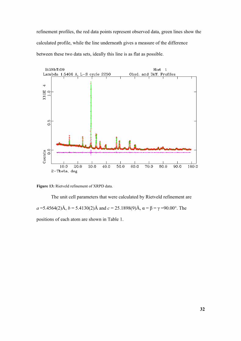
Table 1: Unit cell data for Bi3NbTiO9. aFixed to define origin of the polar axis.
The values for the unit cell obtained by Rietveld refinement correspond well
to the figures on which the refinement was based. The published figures, that were
used as a basis for refinement, are a = 5.440(7)Å, b = 5.394(7)Å and c = 25.099(5)Å,
33
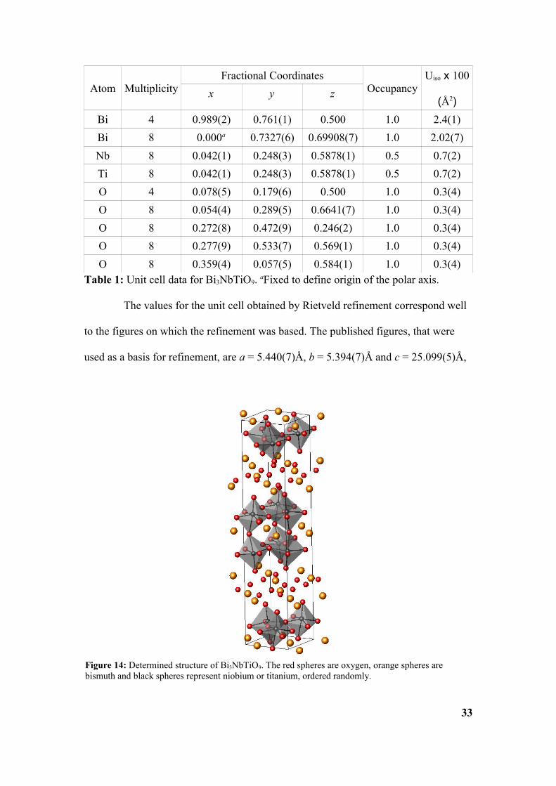
Figure 14: Determined structure of Bi3NbTiO9. The red spheres are oxygen, orange spheres are bismuth and black spheres represent niobium or titanium, ordered randomly.
α = β = γ =90.00°16. The data from the Rietveld refinement gives rise to the unit cell
described by Figure 14.
3.2 Bi 4Ti3O12 Characterisation
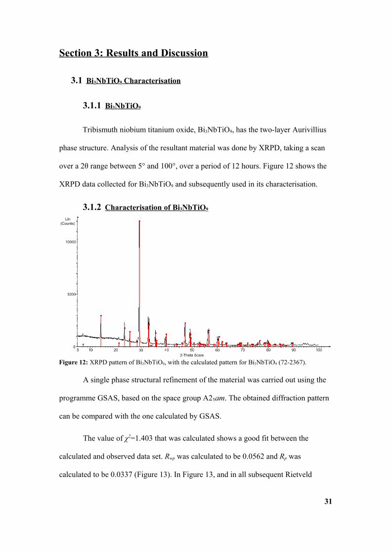
3.2.1 Bi 4Ti3O12
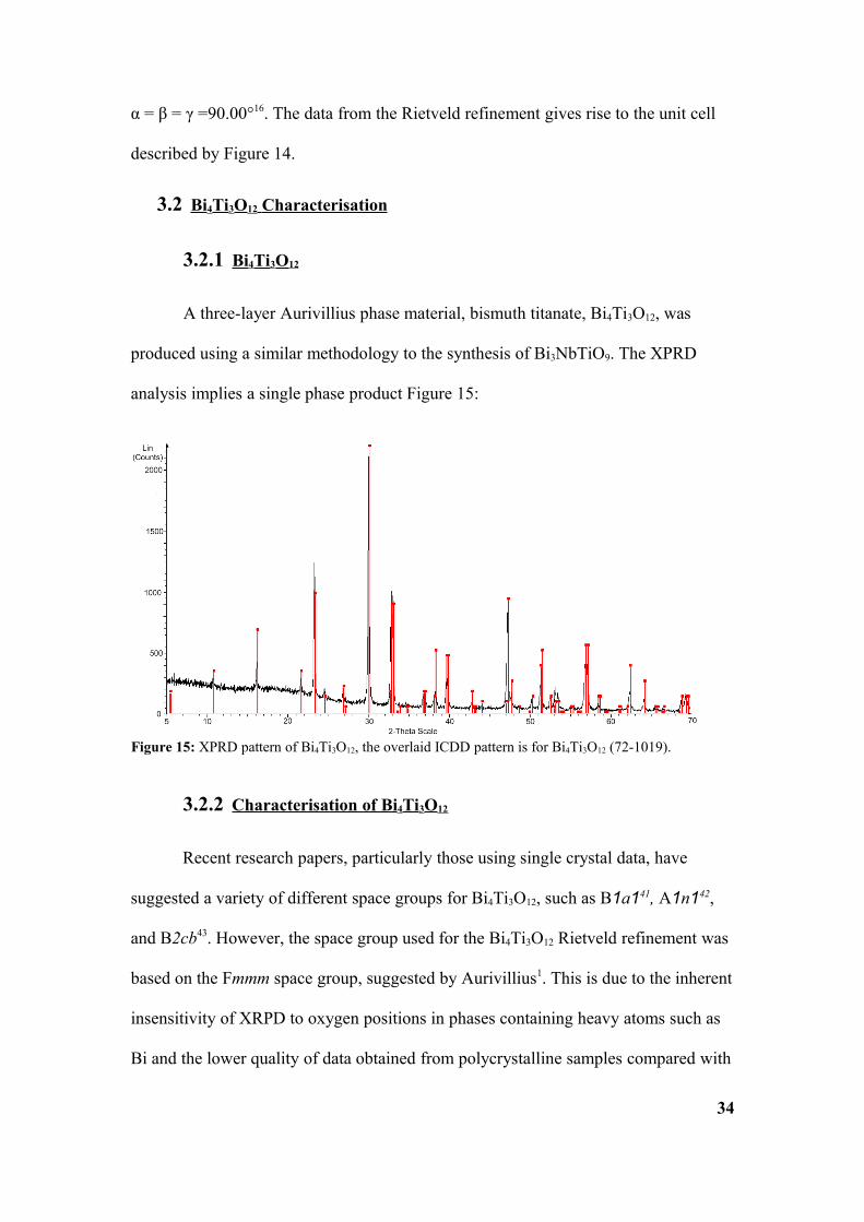
A three-layer Aurivillius phase material, bismuth titanate, Bi4Ti3O12, was
produced using a similar methodology to the synthesis of Bi3NbTiO9. The XPRD
analysis implies a single phase product Figure 15:
3.2.2 Characterisation of Bi 4Ti3O12
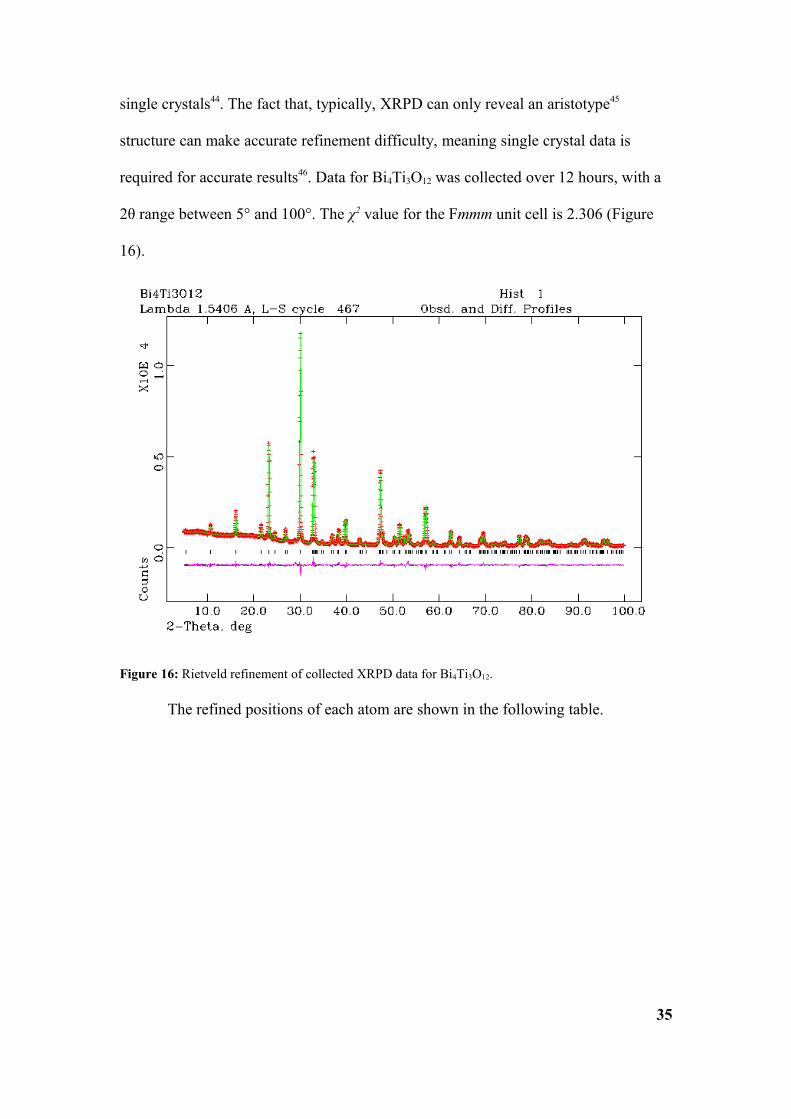
Recent research papers, particularly those using single crystal data, have
suggested a variety of different space groups for Bi4Ti3O12, such as B1a141, A1n142,
and B2cb43. However, the space group used for the Bi4Ti3O12 Rietveld refinement was
based on the Fmmm space group, suggested by Aurivillius1. This is due to the inherent
insensitivity of XRPD to oxygen positions in phases containing heavy atoms such as
Bi and the lower quality of data obtained from polycrystalline samples compared with
34
Figure 15: XPRD pattern of Bi4Ti3O12, the overlaid ICDD pattern is for Bi4Ti3O12 (72-1019).
single crystals44. The fact that, typically, XRPD can only reveal an aristotype45
structure can make accurate refinement difficulty, meaning single crystal data is
required for accurate results46. Data for Bi4Ti3O12 was collected over 12 hours, with a
2θ range between 5° and 100°. The χ2 value for the Fmmm unit cell is 2.306 (Figure
16).
The refined positions of each atom are shown in the following table.
35
Figure 16: Rietveld refinement of collected XRPD data for Bi4Ti3O12.
The calculated unit cell parameters are a = 5.4043(1)Å, b = 5.4432(1)Å and
c = 32.785(1)Å, α = β = γ =90.00°. The values that were suggested by Aurivillius
(1949) are quite similar, being a = 5.41Å, b = 5.448Å and c = 32.84Å,
α = β = γ =90.00°.
3.3 Characterisations of Bi 5Fex+1Ti3-xO15
36
Figure 17: Graphical representation of the structure of Bi4Ti3O12. The red spheres are oxygen, orange spheres are bismuth and black spheres represent titanium.
3.3.1 Bi 5FeTi3O15
The compound Bi5Ti3FeO15 is one example of a whole family of Aurivillius
phase materials which are based on bismuth titanate, with iron acting as a magnetic
ion with the general formula Bix+4FexTi3O3(x+4). This four layer member of the bismuth
iron titanate family (where x=1) has a proportion of its B sites doped with Fe. The
ferroelectric behaviour of Bi5FeTi3O15 has been relatively well documented47-52.47,48,
49,50,51,52
3.3.1.1 Characterisation of Bi 5FeTi3O15
X-ray powder diffraction data for Bi5FeTi3O15 was carried out over a period of
12 hours, with a 2θ range from 5° to 95°. Structural data for the Rietveld refinement
of Bi5FeTi3O15 was based on structural data provided by previous work, based on the
37
Figure 18: Rietveld refinement of Bi5FeTi3O15.
A21am space group53. The refinement profile had a χ2 value of 1.224, which indicates
a good fit between the observed and calculated data sets (Figure 18).
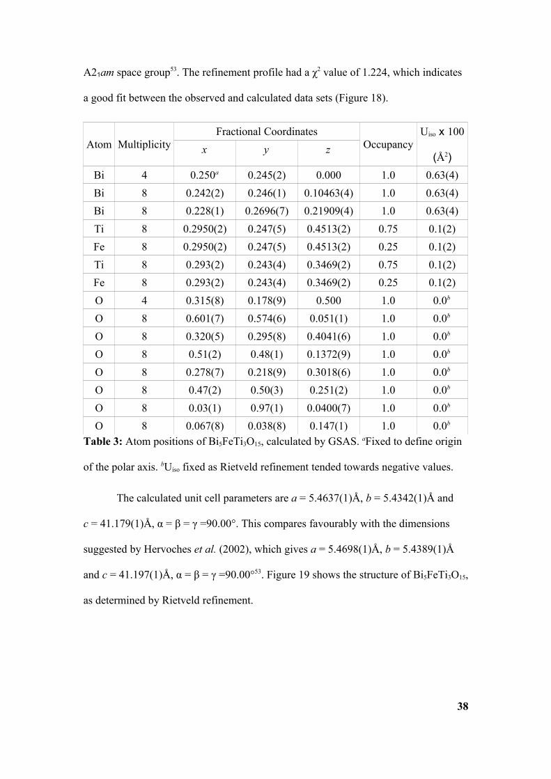
Table 3: Atom positions of Bi5FeTi3O15, calculated by GSAS. aFixed to define origin
of the polar axis. bUiso fixed as Rietveld refinement tended towards negative values.
The calculated unit cell parameters are a = 5.4637(1)Å, b = 5.4342(1)Å and
c = 41.179(1)Å, α = β = γ =90.00°. This compares favourably with the dimensions
suggested by Hervoches et al. (2002), which gives a = 5.4698(1)Å, b = 5.4389(1)Å
and c = 41.197(1)Å, α = β = γ =90.00°53. Figure 19 shows the structure of Bi5FeTi3O15,
as determined by Rietveld refinement.
38
The Bi5FeTi3O15 sample was placed into the PPMS and cooled to 4K and a
field of 1000Oe was applied, before the sample was allowed to heat up to room
temperature. By plotting the magnetic dipole moment in electromagnetic units against
temperature in Kelvin (Figure 20) it can be seen that the magnetic dipole moment
increases as temperature decreases, which is clearly a sign of paramagnetic behaviour.
By plotting χ against temperature in Kelvin, a plot is obtained that can be interpreted
by using the Curie-Weiss law. The Curie-Weiss law:
χ= CT−
To more accurately calculate the magnetic properties it is necessary to add a constant
to represent temperature independent properties, such as the inherent diamagnetism of
paired electrons. Adding a constant to the Curie-Weiss law gives:
39
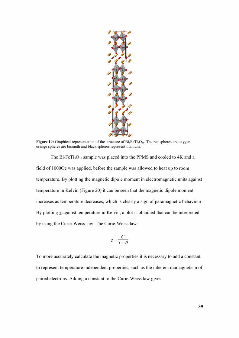
Figure 19: Graphical representation of the structure of Bi5FeTi3O15. The red spheres are oxygen, orange spheres are bismuth and black spheres represent titanium.
χ= CT−
χ0
Where χ is the magnetic susceptibility, T is the temperature (in K) and θ represents
the critical temperature. The constants C and χ0 represent the material-specific Curie
constant and the temperature independent magnetic characteristics, respectively. The
calculated variables tell us several things about the magnetic properties of
Bi5FeTi3O15. A positive θ indicates that the predominant interactions are
ferromagnetic even though magnetic ordering may not occur. A negative θ implies
predominantly anti-ferromagnetic interactions.
The fitted curve (the red
line in Figure 20) for χ plotted
against T, has a R2 value of
0.99982, which indicates a high
goodness of fit. The equation of
the fitted curve gives a θ value of
-5.282K, indicative of latent anti-
ferromagnetic character. With a
value of C determined to be 1.573x10⁻⁵, the paramagnetic moment has been calculated
to be 3.164μB. This is lower than the calculated and experimental values for the
magnetic moment of Fe3+, 5.92μB and 5.9μB54, respectively. This would appear to
indicate that the Fe cations adopt an intermediate spin-state55, which has also been
suggested in other iron-substituted Aurivillius phase materials, such as
Bi2Sr2Nb2.5Fe0.5O1256.
40
Figure 20: Graph showing the relationship between magnetic susceptibility and temperature for Bi5FeTi3O15.
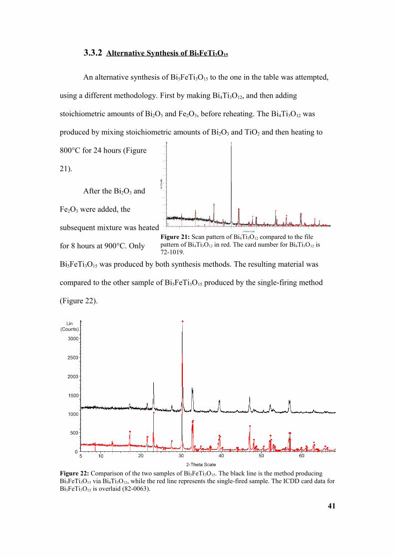
3.3.2 Alternative Synthesis of Bi 5FeTi3O15
An alternative synthesis of Bi5FeTi3O15 to the one in the table was attempted,
using a different methodology. First by making Bi4Ti3O12, and then adding
stoichiometric amounts of Bi2O3 and Fe2O3, before reheating. The Bi4Ti3O12 was
produced by mixing stoichiometric amounts of Bi2O3 and TiO2 and then heating to
800°C for 24 hours (Figure
21).
After the Bi2O3 and
Fe2O3 were added, the
subsequent mixture was heated
for 8 hours at 900°C. Only
Bi5FeTi3O15 was produced by both synthesis methods. The resulting material was
compared to the other sample of Bi5FeTi3O15 produced by the single-firing method
(Figure 22).
41
Figure 21: Scan pattern of Bi4Ti3O12 compared to the file pattern of Bi4Ti3O12 in red. The card number for Bi4Ti3O12 is 72-1019.
Figure 22: Comparison of the two samples of Bi5FeTi3O15. The black line is the method producing Bi5FeTi3O15 via Bi4Ti3O12, while the red line represents the single-fired sample. The ICDD card data for Bi5FeTi3O15 is overlaid (82-0063).
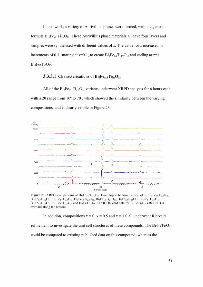
In this work, a variety of Aurivillius phases were formed, with the general
formula Bi5Fex+1Ti3-xO15. These Aurivillius phase materials all have four layers and
samples were synthesised with different values of x. The value for x increased in
increments of 0.1, starting at x=0.1, to create Bi5Fe1.1Ti2.9O15 and ending at x=1,
Bi5Fe2Ti2O15.
3.3.3.1 Characterisations of Bi 5Fex+1Ti3-xO15
All of the Bi5Fex+1Ti3-xO15 variants underwent XRPD analysis for 6 hours each
with a 2θ range from 10º to 70º, which showed the similarity between the varying
compositions, and is clearly visible in Figure 23:
In addition, compositions x = 0, x = 0.5 and x = 1.0 all underwent Rietveld
refinement to investigate the unit cell structures of these compounds. The Bi5FeTi3O15
could be compared to existing published data on this compound, whereas the
42
Figure 23: XRPD scan patterns of Bi5Fe1+xTi3-xO15. From top to bottom, Bi5Fe2Ti2O15, Bi5Fe1.9Ti2.1O15, Bi5Fe1.8Ti2.2O15, Bi5Fe1.7Ti2.3O15, Bi5Fe1.6Ti2.4O15, Bi5Fe1.5Ti2.5O15, Bi5Fe1.4Ti2.6O15, Bi5Fe1.3Ti2.7O15, Bi5Fe1.2Ti2.8O15, Bi5Fe1.1Ti2.9O15 and Bi5FeTi3O15. The ICDD card data for Bi5FeTi3O15 (38-1257) is overlaid along the bottom.
refinement of the Bi5Fe1.5Ti2.5O15 and Bi5Fe2Ti2O15 compositions provided new data on
these previously unreported compounds, opening up new lines of inquiry.
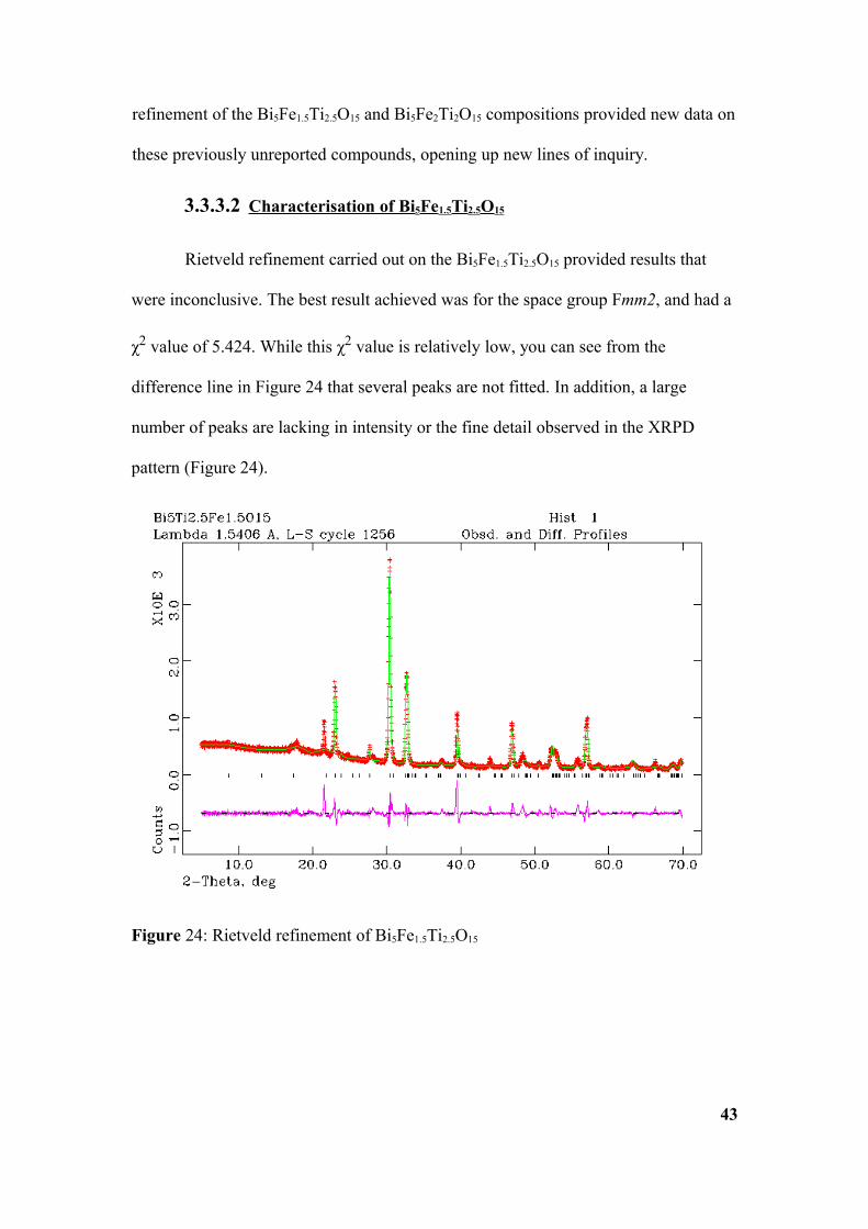
3.3.3.2 Characterisation of Bi 5Fe1.5Ti2.5O15
Rietveld refinement carried out on the Bi5Fe1.5Ti2.5O15 provided results that
were inconclusive. The best result achieved was for the space group Fmm2, and had a
χ2 value of 5.424. While this χ2 value is relatively low, you can see from the
difference line in Figure 24 that several peaks are not fitted. In addition, a large
number of peaks are lacking in intensity or the fine detail observed in the XRPD
pattern (Figure 24).
43
Figure 24: Rietveld refinement of Bi5Fe1.5Ti2.5O15
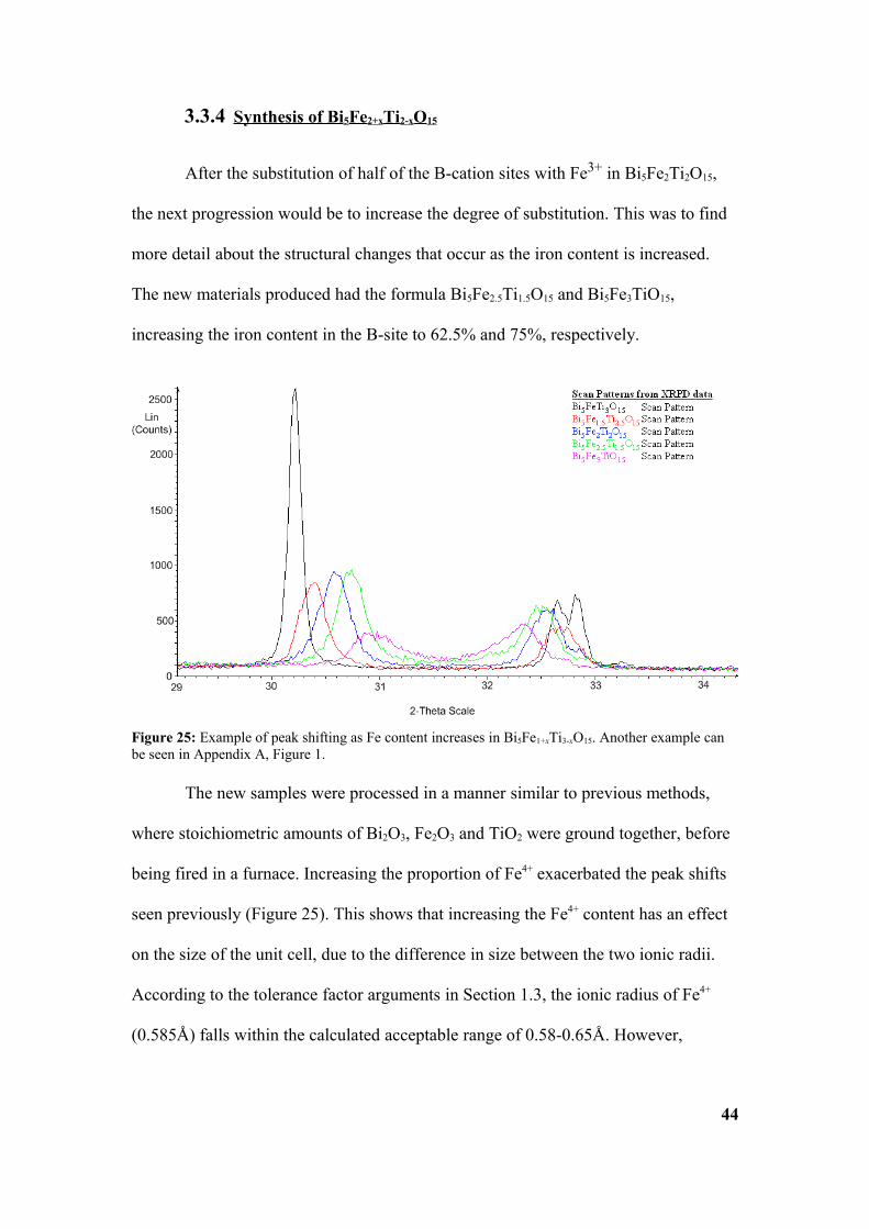
3.3.4 Synthesis of Bi 5Fe2+xTi2-xO15
After the substitution of half of the B-cation sites with Fe3+ in Bi5Fe2Ti2O15,
the next progression would be to increase the degree of substitution. This was to find
more detail about the structural changes that occur as the iron content is increased.
The new materials produced had the formula Bi5Fe2.5Ti1.5O15 and Bi5Fe3TiO15,
increasing the iron content in the B-site to 62.5% and 75%, respectively.
The new samples were processed in a manner similar to previous methods,
where stoichiometric amounts of Bi2O3, Fe2O3 and TiO2 were ground together, before
being fired in a furnace. Increasing the proportion of Fe4+ exacerbated the peak shifts
seen previously (Figure 25). This shows that increasing the Fe4+ content has an effect
on the size of the unit cell, due to the difference in size between the two ionic radii.
According to the tolerance factor arguments in Section 1.3, the ionic radius of Fe4+
(0.585Å) falls within the calculated acceptable range of 0.58-0.65Å. However,
44
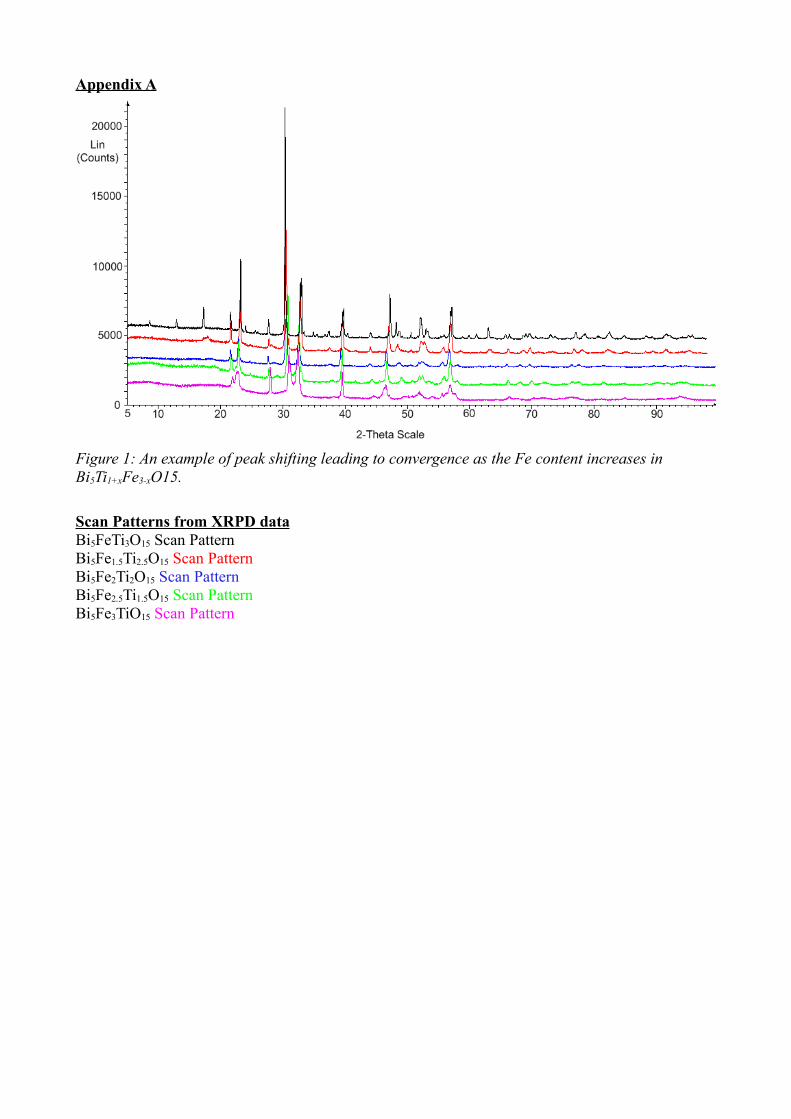
Figure 25: Example of peak shifting as Fe content increases in Bi5Fe1+xTi3-xO15. Another example can be seen in Appendix A, Figure 1.
without the acquisition of further data, the exact effects of increasing the iron content
are unknown, including the possibility of oxygen deficiencies occurring, which would
give a possible non-stoichiometric formula of Bi5Fe3TiO15-δ.
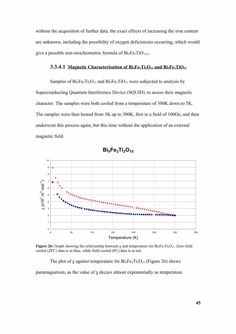
3.3.4.1 Magnetic Characterisation of Bi 5Fe2Ti2O15 and Bi5Fe3TiO15
Samples of Bi5Fe2Ti2O15 and Bi5Fe3TiO15 were subjected to analysis by
Superconducting Quantum Interference Device (SQUID), to assess their magnetic
character. The samples were both cooled from a temperature of 300K down to 5K.
The samples were then heated from 5K up to 300K, first in a field of 100Oe, and then
underwent this process again, but this time without the application of an external
magnetic field.
The plot of χ against temperature for Bi5Fe2Ti2O15 (Figure 26) shows
paramagnetism, as the value of χ decays almost exponentially as temperature
45
Figure 26: Graph showing the relationship between χ and temperature for Bi5Fe2Ti2O15. Zero-field cooled (ZFC) data is in blue, while field cooled (FC) data is in red.
Bi5Fe2Ti2O15
0
1
2
3
4
5
6
7
8
9
10
0 50 100 150 200 250 300 350
Temperature (K)
χ (x
107 m
3 mol
-1)
increases. However, the FC data retains a gradient, whereas the ZFC data reaches a
plateau.
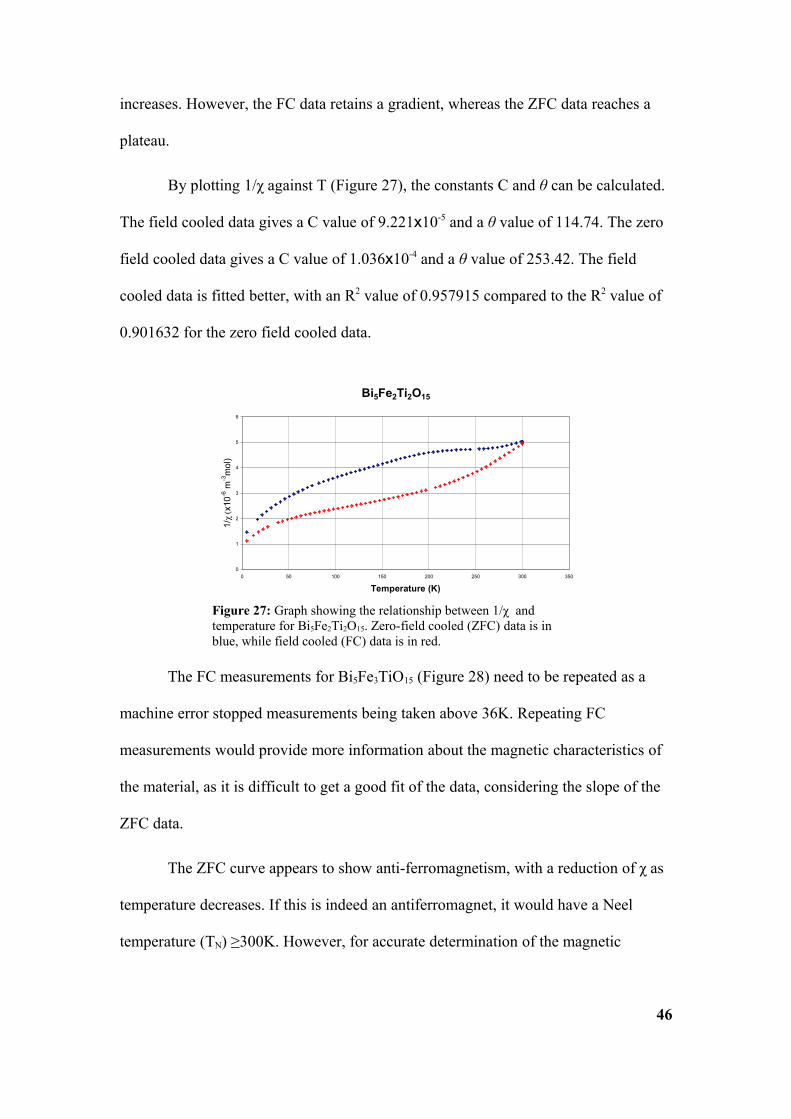
By plotting 1/χ against T (Figure 27), the constants C and θ can be calculated.
The field cooled data gives a C value of 9.221x10⁻⁵ and a θ value of 114.74. The zero
field cooled data gives a C value of 1.036x10⁻⁴ and a θ value of 253.42. The field
cooled data is fitted better, with an R2 value of 0.957915 compared to the R2 value of
0.901632 for the zero field cooled data.
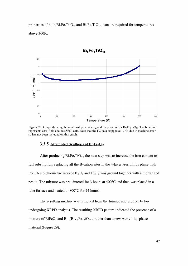
The FC measurements for Bi5Fe3TiO15 (Figure 28) need to be repeated as a
machine error stopped measurements being taken above 36K. Repeating FC
measurements would provide more information about the magnetic characteristics of
the material, as it is difficult to get a good fit of the data, considering the slope of the
ZFC data.
The ZFC curve appears to show anti-ferromagnetism, with a reduction of χ as
temperature decreases. If this is indeed an antiferromagnet, it would have a Neel
temperature (TN) ≥300K. However, for accurate determination of the magnetic
46
Figure 27: Graph showing the relationship between 1/χ and temperature for Bi5Fe2Ti2O15. Zero-field cooled (ZFC) data is in blue, while field cooled (FC) data is in red.
Bi5Fe2Ti2O15
0
1
2
3
4
5
6
0 50 100 150 200 250 300 350
Temperature (K)
1/χ
( x10
-6 m
-3m
ol)
properties of both Bi5Fe2Ti2O15 and Bi5Fe3TiO15, data are required for temperatures
above 300K.
3.3.5 Attempted Synthesis of Bi 5Fe4O15
After producing Bi5Fe3TiO15, the next step was to increase the iron content to
full substitution, replacing all the B-cation sites in the 4-layer Aurivillius phase with
iron. A stoichiometric ratio of Bi2O3 and Fe2O3 was ground together with a mortar and
pestle. The mixture was pre-sintered for 3 hours at 400°C and then was placed in a
tube furnace and heated to 800°C for 24 hours.
The resulting mixture was removed from the furnace and ground, before
undergoing XRPD analysis. The resulting XRPD pattern indicated the presence of a
mixture of BiFeO3 and Bi12(Bi0.5,Fe0.5)O19.5, rather than a new Aurivillius phase
material (Figure 29).
47
Bi5Fe3TiO15
0
0.5
1
1.5
2
2.5
3
3.5
0 50 100 150 200 250 300 350
Temperature (K)
χ (x
107 m
3 mol
-1)
Figure 28: Graph showing the relationship between χ and temperature for Bi5Fe3TiO15. The blue line represents zero-field cooled (ZFC) data. Note that the FC data stopped at ~36K due to machine error, so has not been included on this graph.
3.4 Attempted Syntheses of Bi 5Mn1+xTi3-xO15
The formation of another 4-layer Aurivillius phase with the same structure as
Bi5Fey+1Ti3-yO15, except with Mn3+/4+ ions instead of Fe3+/4+ ions, Bi5Mnx+1Ti3-xO15 was
attempted. Again, the value of x was varied between 0 and 1, again increasing by
intervals of 0.1, in an attempt to produce samples ranging from Bi5MnTi3O15 to
Bi5Mn2Ti2O15. The Mn-doped samples were fired in similar conditions to the Fe-
doped samples. Reaction conditions were similar to those of Bi5Fe1+xTi3-xO15, as
outlined by previous studies50,57.
Samples were fired at 850°C for 8 hours in oxygen under atmospheric
pressure. The samples were then ground for 15 minutes. The samples were
subsequently fired at 900°C for 6 hours, again in oxygen under atmospheric pressure.
The samples were then ground and before the treatment at 900°C was then repeated.
48
Figure 29: XRPD pattern of attempted Bi5Fe4O15 sample, the vertical blue lines show the patterns on file for BiFeO3 (71-2494) and the red lines are associated with Bi12(Bi0.5,Fe0.5)O19.5 (77-0568).
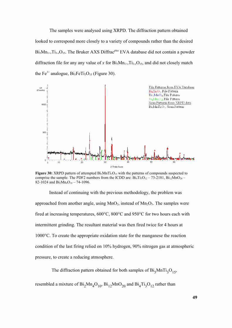
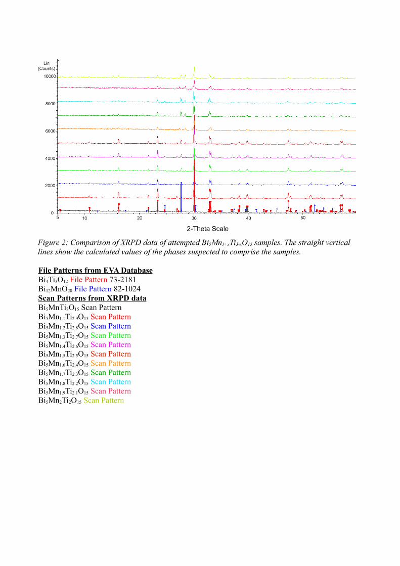
The samples were analysed using XRPD. The diffraction pattern obtained
looked to correspond more closely to a variety of compounds rather than the desired
Bi5Mn1+xTi3-xO15. The Bruker AXS Diffracplus EVA database did not contain a powder
diffraction file for any any value of x for Bi5Mn1+xTi3-xO15, and did not closely match
the Fe3+ analogue, Bi5FeTi3O15 (Figure 30).
Instead of continuing with the previous methodology, the problem was
approached from another angle, using MnO2, instead of Mn2O3. The samples were
fired at increasing temperatures, 600°C, 800°C and 950°C for two hours each with
intermittent grinding. The resultant material was then fired twice for 4 hours at
1000°C. To create the appropriate oxidation state for the manganese the reaction
condition of the last firing relied on 10% hydrogen, 90% nitrogen gas at atmospheric
pressure, to create a reducing atmosphere.
The diffraction pattern obtained for both samples of Bi5MnTi3O15,
resembled a mixture of Bi2Mn4O10, Bi12MnO20 and Bi4Ti3O12 rather than
49
Figure 30: XRPD pattern of attempted Bi5MnTi3O15 with the patterns of compounds suspected to comprise the sample. The PDF2 numbers from the ICDD are: Bi4Ti3O12 – 73-2181, Bi12MnO20 – 82-1024 and Bi2Mn4O10 – 74-1096.
Bi5MnTi3O15, using diffraction data from the EVA database. Diffraction patterns for
Bi5Mn1+xTi3-xO15 are included in Appendix A.
While Mn3+ appears to fulfil the criteria for successful (and significant) B-
site substitution, the methodology outlined would appear to be unsuccessful. Although
manganese cation substitution into Aurivillius phase structures is technically possible
(as in the radius and charge of Mn3+ would make it a suitable cation for the position),
without further verification of these papers by another source, it would suggest that
the most prudent course of action would be to remain incredibly sceptical of the
findings of these papers.
Several papers advise the use of a modest excess of Bi2O3 to offset the losses
of Bi2O3. Also, as Bi2O3 has a melting point of approximately 825°C, the excess
molten Bi2O3 can allow the reaction to be self-fluxed. Considering the reaction
conditions, extra Bi2O3 can reliably form a range of compounds with TiO2 and Mn2O3,
including a 3-layer Aurivillius phase, Bi4Ti3O12, which would make the
characterisation of any collected data more difficult.
50
Section 4: Conclusions and Further Work
4.1 Conclusions
The production and synthesis of both Bi3TiNbO9 and Bi4Ti3O12 is a relatively
routine procedure, when using the ceramic method. Substitution of Fe3+/4+ into the four
layer Aurivillius phase structure is possible to levels beyond those previously
reported. However, the modifications to the structure that occur are possibly outside
those that are calculable by GSAS refinement of powder data.
There are multiple possibilities for the change between the Bi5Fe1+xTi3-xO15
phases as the Fe:Ti proportion increases. To determine how the change in structure
takes place will require more data and possibly the use of additional techniques, as
outlined in the section entitled 'Further Work'.
The inability to produce Bi5Mn1+xTi3-xO15 raises doubts about previous
papers50,57. Based on the data collected as part of this project it is unlikely to be
possible using the methodologies outlined. The papers in question certainly require a
greater degree of scrutiny to ascertain the veracity of their conclusions.
However, the possibility to achieve significant manganese substitution should
not be overlooked because of this. The techniques used may require more severe
reaction conditions, or possibly co-substitution with another cation, in either the A or
B sites as manganese ions typically prefer a higher oxidation state than Mn3+.
It is therefore clear that bismuth layer structure ferroics contain a great deal of
potential. Their flexibility and versatility should not be overlooked when designing
51
materials for various applications. In the future, it may be possible to tailor Aurivillius
phase structure materials for specific uses.
4.2 Further Work
Further work should focus on obtaining more information about the structure
of the Bi5Fe1+xTi3-xO15 phases where x is greater than 0. While the unit cell structure of
the Bi5FeTi3O15 phase is relatively well-documented the new phases derived from this
material may have diverged in a variety of ways.
Single crystal X-ray diffraction or neutron diffraction may be necessary to
eliminate various permutations of the unit cell, for instance the tilting and twisting of
the (Ti, B)O6 can make accurate determination of the unit cells of various Aurivillius
phases more difficult. A degree of structural degeneracy could account for the
difficulty in refining the unit cells.
Another possibility would be that the materials with increased iron content
create an intergrowth phase, containing an increasing proportion of BiFeO3 sub-
layers. In this instance electron microscopy techniques, such as Scanning Electron
Microscopy (SEM), or Transmission Electron Microscopy (TEM) may be necessary
to determine the layer structure of the newly-created phases. Electron microscopy has
been used for this purpose, to great effect, in observing the layering in materials such
as Bi7Ti4NbO2158.
After submission, Mössbauer spectroscopy is due to be carried out on the
Bi5FeTi3O15, Bi5Fe2Ti2O15, Bi5Fe3TiO15 and Bi5Fe4O15 samples. Appendix B contains
information on the Mössbauer spectroscopy technique. The primary information that
is obtainable from Mössbauer spectroscopy is the oxidation state of the Fe cations.
52
Additionally, information about whether or not electron exchange is occurring and
magnetic interactions can be collected, amongst other details.
Further work should also consider the substitutions of other magnetic ions and
also possibilities involving co-substitution. The substitution for other ions in the place
of Bi3+ should also be attempted to alter the properties of Aurivillius phase materials.
Additional lines of enquiry would include increasing the number of layers within the
Aurivillius phase structure and using intergrowth behaviours to modify the properties
of materials.
As well as cations, the anion sites of bismuth layer structure can have the
oxygen replaced by other anions, as witnessed in Bi2TiO4F2 and Bi2NbO5F59. This
provides another option in altering the properties of the layered structure. In
conclusion, the versatility of Aurivillius phase materials provides a wealth of potential
and opportunity for any chemist.
53
1B. Aurivillius, (1949), Arkiv for Kemi, Volume 1, Iss. 6, p499-5122K. Aizu, (1969), Journal of the Physical Society of Japan, Vol. 27, p387
3S.C. Abrahams, (1971), Materials Research Bulletin, Vol. 6, p881-890
4N.A. Hill, A. Filippetti, (2002), Journal of Magnetism and Magnetic Materials,
Volume 242, p976
5H. Schmid, (1994), Bulletin of Material Sciences, Volume 17, Iss. 7, p1411
6H. Schmid, (1973), International Journal of Magnetism, Volume 4, p3377E. Ascher, (1973), International Journal of Magnetism, Volume 5, p287
Volume 6, p1029-104616J.G. Thompson, A.D. Rae, R.L. Withers and D.C. Craig, (1990), Acta
Crystallographica, Volume B47, p174
17J.G. Thompson, R.L. Withers and A.D. Rae, (1991), Journal of Solid State
Chemistry, Volume 94, Issue 2, p404
18D.I. Khomskii, (2005), Journal of Magnetism and Magnetic Materials, Vol. 306,
p1-819P.A. Cox, Insulating Oxides, In J.S. Rowlinsin, M.L.H. Green, J. Halpern, S.V. Ley,
T. Mukaiyama, R.L. Schowen, J.M. Thomas, A.H. Zewail, editors, Transition Metal
Oxides: An Introduction to Their Electronic Structure and Properties, 1st Ed.
(Paperback), Biddles Ltd., 1995, p149-153
20P. Day, M.T. Hutchings, E. Janke, P.J. Walker, (1979), Journal of the Chemical
Society: Chemical Communications, Issue 16, p71121G. Matsumoto, (1970), Journal of the Physical Society of Japan, Volume 23,
Number 9, p60622E.O. Wollan, W.C. Koehler, (1955), Physical Review, Volume 100, Number 2, p54523C. Wang, J. Wang, Z. Gai, (2007), Scripta Materiala, Vol. 57, p789-79224E.C. Subbarao, (1962), Journal of the American Ceramic Society, Vol. 45, Iss. 4,
p166
25R.A. Armstrong, R.E. Newnham, (1972), Material Research Bulletin, Vol. 7, p1025
26M. Tripathy, R. Mani, J. Gopalakrishnan, (2007), Material Research Bulletin, Vol.
42, p950
27H. Hara, Y. Noguchi, M. Miyayama, (2004), Key Engineering Materials, Vol. 269,
p27
28B. Frit, J. Mercurio, (1992), Journal of Alloys and Compounds, Vol. 188, p27
29J. Gopalakrishnan, A. Ramanan, C. Rao, D. Jefferson, D. Smith, (1984), Journal of
Solid State Chemistry, Vol. 55, p101
30M. Miyayama, (2006), Journal of the Ceramic Society of Japan, Vol. 114, Iss. 7,
p583-58931A. Lisińska-Czejak, D. Czejak, M.J.M. Gomes, M.F. Kupriamov, (1999), Journal of
the European Ceramic Society, Iss. 19, p969 32M.M. Woolfson, An Introduction to X-ray Crystallography, 2nd Ed., Cambridge
University Press, 199733ICDD, http://www.icdd.com/ , accessed 23/08/0834A.C. Larson and R.B. Von Dreele, (2000), General Structure Analysis System
(GSAS), Los Alamos National Laboratory Report LAUR 86-748
B. H. Toby, (2001), EXPGUI, a graphical user interface for GSAS, Journal Of
Applied Crystallography, Vol. 34, p210
35ICSD, http://cds.dl.ac.uk/cds/datasets/crys/icsd/llicsd.html , accessed 23/08/0836H.M. Rietveld, (1967), Acta Crystallographica, Volume 22, p15137J. Crangle, The Magnetic Properties of Solids, 1st Ed., Edward Arnold: London,
Aquino, L.E. Fuentes-Cobas, (2004), Revista Mexicana de Fisico, Volume 50, p42-4543P. Lightfoot, C.H. Hervoches, (2003), Proceedings of the 10th International
Ceramics Congress, Volume 10, p623-63044J.G. Thompson, R.L. Withers, A.C. Willis, A.D. Rae, (1990), Acta
Crystallographica, Volume B4, p474-487
45Megaw H., (1973), Crystal Structures, London: W.B. Saunders, p. 216, 28246R.H. Mitchell, Perovskites: Modern and Ancient, 1st Ed., Almaz Press: Thunder Bay,
200247X.W. Dong, K.F. Wang, J.G. Wan, J.S. Zhu, and J. Liu, (2008), Journal of Applied
Physics, Volume 10348S. Zhang, Y. Chen, Z. Liu, N. Ming, J. Wang, G. Cheng, (2005), Journal of Applied
Physics, Volume 97
49A. Snedden, C.H. Hervoches, P. Lightfoot, (2003), Physical Review B, Volume 6750S. Ahn, Y. Noguchi, M. Miyayama, T. Kudo, (2000), Materials Research Bulletin,
Figure 2: Comparison of XRPD data of attempted Bi5Mn1+xTi3-xO15 samples. The straight vertical lines show the calculated values of the phases suspected to comprise the samples.
Figure 3: Close up of the XRPD data of attempted Bi5Mn1+xTi3-xO15 samples. The straight vertical lines show the calculated values of the phases suspected to comprise the samples.
Appendix B: M ö ssbauer Spectroscopy
The Mössbauer Effect
Mössbauer spectroscopy is an analytical technique that is used to determine the magnetic
and time-dependent properties of a material by the effects of recoilless gamma ray emission and
absorption. The Mössbauer effect is based on the resonant absorption of gamma rays in crystalline
structures.
A nuclei can occupy a variety of energy levels, and it is possible to split or alter these energy
levels based on the surrounding electronic and magnetic environment, however these hyperfine
interactions with the environment of the nuclei are extremely small and difficult to observe. In a
variety of different circumstances, transitions between different energy levels can be caused or
evidenced by the absorption or emission of a gamma ray.
A free nucleus will undergo a certain degree of recoil in order to conserve momentum, when
absorbing or emitting a gamma ray. A gamma ray that is absorbed and then subsequently emitted
will have less energy, because the recoil of the nucleus results in an overall loss of kinetic energy.
The recoil effect means that there is no resonance of nuclei, the loss of kinetic energy due to the
conservation of momentum needs to be overcome to provide useful resonance effects.
A resonant signal is important because individual nuclei will be moving in random
directions, giving the gamma ray a variety of different energy values based on the Doppler effect.
Overlap between different signals leads to resonance, but with freely moving nuclei this effect is
low because at most only a millionth of the gamma rays have overlapping signals, making this
technique impractical for detecting hyperfine interactions.
However in 1957, Ernst Mössbauer discovered what would be known as the Mössbauer
Effect. When a gamma ray is absorbed by a nucleus in a crystal lattice the recoiling effect is
massively limited as the mass of the entire lattice is much greater than the mass of a single nucleus.
As the recoil of the lattice approaches zero, the difference in energy between absorbed and emitted
gamma rays approaches zero. At zero, the gamma ray absorbed and the gamma ray emitted have the
same energy, and resonance is achieved.
In a cubic environment, if the absorbing and emitting nuclei are identical, then the spectrum
will show a single absorption line. An excited energy level for a nucleus has a finite lifetime before
a gamma ray is emitted. The average lifetime of an excited state prior to gamma ray emission
determines the linewidth of the spectrum. As the natural linewidth of the most commonly used
Mössbauer isotope, 57Fe is approximately 5x10⁻⁹ eV, whereas Mössbauer gamma rays have an
energy of 14.4keV. This difference, of 12 orders of magnitude, gives resolution sufficient to detect
the hyperfine interactions of the nucleus.
Mössbauer Spectroscopy
By oscillating a radioactive source towards and away from the target material at a low
velocity ( a few millimetres per second), the Doppler effect leads to an energy shift of the gamma
ray. This energy shift is minute enough to observe the hyperfine interactions. The oscillating effect
also allows for slight incremental modulation of the gamma ray.
When you get resonant absorption of the gamma ray, i.e. when the gamma ray energy
matches an energy level transition of the sample material, you can see a peak in the spectra.
Obviously, the sample has to be thin enough to allow the gamma rays to pass through. The energy
levels of the absorbing nuclei are altered by their environment in three main ways, namely, isomer
shift, magnetic splitting and quadrupole splitting.
Differences between the s-electron environments of the source and the receiver produces a
shift in the resonance energy. The shift in transition energy, caused by this difference in electron
charge density, is what is known as isomer shift. This shift is relative to a known absorption, it
cannot be measured directly. Isomer shift is particularly useful for determination of valency state as
ferrous ions have larger positive shifts than ferric ions. This is because ferrous ions have less
influence from the s-electrons at the nucleus due to the screening effects of the greater number of d-
electrons. The formula for calculating isomer shift is given by the formula belowi:
=Ze2 R2 c50 E [a 0−s0][R
R ] mm s−1
Where Z is the atomic number, e is the electronic charge, R is the effective nuclear radius, c
is the speed of light, Eγ is the energy of the Mössbauer gamma ray, the ρa(0) and ρs(0) terms are the
total electron densities at the nucleus for absorber and source, respectively and ΔR = Rexcited –
Rground.
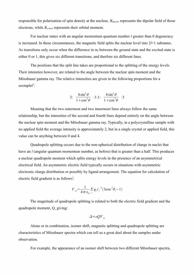
Magnetic splitting is a result of Zeeman splitting, the dipolar interaction with a magnetic
field experienced by the nuclear spin moment. The magnetic field experienced by the nucleus is
given by:
Beff =BcontactBdipolarBorbitalBapplied
As you can see the effective magnetic field is the total combination of the atoms own forces
(in brackets) and an applied magnetic field. Bcontact is the result of spin on the electrons that are
responsible for polarisation of spin density at the nucleus. Bdipolar represents the dipolar field of those
electrons, while Borbital represents their orbital moment.
For nuclear states with an angular momentum quantum number l greater than 0 degeneracy
is increased. In these circumstances, the magnetic field splits the nuclear level into 2l+1 substates.
As transitions only occur when the difference in ml between the ground state and the excited state is
either 0 or 1, this gives six different transitions, and therfore six different lines.
The positions that the split line takes are proportional to the splitting of the energy levels.
Their intensties however, are related to the angle between the nuclear spin moment and the
Mössbauer gamma ray. The relative intensities are given in the following proportions for a
sextupletii:
3:4 sin2
1cos2:1:1:
4 sin21cos2
:3
Meaning that the two outermost and two innermost lines always follow the same
relationship, but the intensities of the second and fourth lines depend entirely on the angle between
the nuclear spin moment and the Mössbauer gamma ray. Typically, in a polycrystalline sample with
no applied field the average intensity is approximately 2, but in a single crystal or applied field, this
value can be anything between 0 and 4.
Quadrupole splitting occurs due to the non-spherical distribution of charge in nuclei that
have an l (angular quantum momentum number, as before) that is greater than a half. This produces
a nuclear quadrupole moment which splits energy levels in the presence of an asymmetrical
electrical field. An asymmetric electric field typically occurs in situations with asymmetric
electronic charge distribution or possibly by ligand arrangement. The equation for calculation of
electric field gradient is as followsi:
V zz=1
40i
qi r i−33cos 2i−1
The magnitude of quadrupole splitting is related to both the electric field gradient and the
quadrupole moment, Q, giving:
=eQV zz
Alone or in combination, isomer shift, magnetic splitting and quadrupole splitting are
characteristics of Mössbauer spectra which can tell us a great deal about the samples under
observation.
For example, the appearance of an isomer shift between two different Mössbauer spectra,
taken before and after calcination, can be indicative of a second compound with a different
oxidation state being formed. Similarly, if an atom moves from it's central position in a unit cell
there will be a corresponding change in the electronic charge distribution, making it asymmetric and
therefore leading to quadrupole splitting. Obviously, the property indicated by magnetic splitting is
a display of whether or not a sample is magnetically ordered.
i R.V. Parish, Mössbauer Spectroscopy and the Chemical Bond; In: D.P.E. Dickson, F.J. Berry,
editors, Mössbauer Spectroscopy, 1st Ed., Cambridge University Press, 1986, p21
ii M.F. Thomas, C.E. Johnson, Mössbauer Spectroscopy of Magnetic Solids; In: D.P.E. Dickson,