Paper ID #32026

Synthesis of a Correcting Equation for 3 Point Bending Test Data

Mr. Jacob Allen Poremski, Geneva College

Jacob A. Poremski is currently an undergraduate student at Geneva College. He is a senior pursuing aBachelor of Science in Engineering (Concentration in Mechanical Engineering) and a Bachelor of Sciencein Applied Mathematics. He has worked as an Apprentice Product Engineering Intern at Kennametal INCduring the summers of 2018 and 2019.

I am interested in the mechanics side of mechanical engineering. More specifically, I seek to pursue acareer that deals with the design, optimization, and analysis of products. My professional developmentat Kennametal over the past two summers has focused on analyzing both the static and fatigue propertiesassociated with products during operation. Verification of results and generating technical analysis reportsfollowed all completed analyses. Currently, I am working on a senior design project focused on the designand analysis of robotic end of arm tooling to help Kennametal automate a specific pick and place processin a manufacturing facility. I seek to attend graduate school to obtain a Master of Science in MechanicalEngineering part time while working full time as a Mechanical Engineer.

Dr. Christopher Charles Jobes P.E., Geneva College

Dr. Jobes is a Professor of Mechanical Engineering at Geneva College in Beaver Falls, Pennsylvania, aProfessional Engineer certified in Pennsylvania with his own consulting company, and is a Research En-gineer for the National Institute for Occupational Safety and Health (NIOSH) Pittsburgh Research Center.He worked for the U. S. Bureau of Mines in control and navigation of a computer-assisted mining machinefrom 1987 through 1997 earning his Professional Engineering certification from Pennsylvania in 1989.Dr. Jobes has since been working for NIOSH in Mining Equipment Safety, Jolting and Jarring Abatementin Mining Machinery, underground refuge alternatives, and Interventions to Enhance Continuous MinerOperator Safety developing Proximity Detection technology. He is currently a Research Engineer study-ing EMI and performing FMEA analyses for underground coal equipment. Dr. Jobes has been teachingin Geneva College’s Engineering Department since 2007 and has been a full-time professor since 2015.His areas of interest lie in Engineering Mechanics, Machine Component Design, FInite Element Analysis,Kinematics, Robotics, Digital Systems Design, Mechanical Vibrations and Control Theory.

c©American Society for Engineering Education, 2020

Synthesis of a Correcting Equation for 3 Point Bending Test Data

Abstract

A frequent requirement of a Mechanics of Deformable Bodies course is for students to complete

an experiment using a compression/tension test fixture incorporating a 3-point flexure fixture.

The prominent goals of such an assignment are to understand the basic concepts of

load/deflection relationships for pure bending situations, to calculate and correlate theoretical

analysis with experimental results, and to use computer software to plot and analyze data. Once

completed, students should be able to compare theoretical and experimental modulus of elasticity

values. The student should then be able to not only determine the type of material used in the 3-

point bending test but also discuss any discrepancies between theoretical and experimental

values.

During the preparation of lab materials for such an experiment, it was noticed that the data

collected from the instrument produced incorrect modulus of elasticity values for all specimens.

Extension values suggested that there was more deflection occurring in the test specimen than

predicted resulting in modulus of elasticity values lower than expected. In fact, the modulus of

elasticity values could be so low that a student could not correctly determine the material type of

the specimen being analyzed. In order to correct the extension data, a system deflection analysis

was initiated.

First, internal displacements occurring within the 3-point flexure fixture members were

determined by calculating the deflections produced during experimental loading. Next, the

remaining sources of internal displacements within the system were investigated with the results

being fitted to a curve. A correction equation with support separation distance, applied load, and

specimen weight as independent variables was generated by summing all the internal

displacements found. The original extension data could then be adjusted by subtracting this

correction displacement. The resulting correction equation was validated using specimens with a

known modulus of elasticity. Successful completion of this project would allow students to

appropriately correct the 3-point bending extension data collected during an experiment and

more accurately calculate an unknown specimen's modulus of elasticity.

Introduction

Typical curricula for students pursuing a degree in an engineering mechanics field includes the

study of load/deflection relationships for certain materials. These relationships include, but are

not limited to, axial, torsional, and lateral loading of members. Deflection equations are

developed during instruction that allows students to calculate the theoretical deflection of objects

so loaded. Regardless of the form these deflection equations take, students can use them to

determine the modulus of elasticity for the material comprising the member, an important

concept when dealing with unknown materials. While some students can grasp the fundamental

concepts of load and deflection just by studying theoretical material, some students learn more

easily by completing hands-on experiments. Students who learn more easily using hands-on

methods are referred to as kinesthetic learners. Whatever mode of learning works best for these

students, all students benefit from performing physical experiments that apply the theoretical

material to a physical experiment. The truth in this fact is because “Over 80 percent of college

faculty use lecture as their primary instructional method. At its core, kinesthetic learning gives

students the opportunity to move out from behind their desks and to interact with their

surroundings” [1]. Therefore, even if laboratory experiments are not required by a traditional

class curriculum, incorporating them is beneficial for illustrating a concept. An additional

benefit is that engineering students may be introduced to the types of load/deflection tests that

they may deal with in their professional careers after graduation.

The strength of a material is inherent in the material itself and must be determined by

experiment. Hibbeler [2] explains, “One of the most important tests to perform in this regard is

the tension or compression test.” There are others but utilizing a 3-point bending test provides

additional benefits. Three of these benefits are due to test specimen geometry, machining

capability, and student instruction. University engineering mechanics laboratories differ

concerning the type and capacity of test equipment available. To test material such as steel using

a tension test, the diameter of the test sample would be determined by the load capacity of the

test equipment available. If the diameter of the test specimen were too large, the test may fail

due to no yielding or fracture occurring. So, if a smaller test specimen is required, it would need

to be machined to a smaller, non-standard, diameter to conduct a successful experiment. Surface

imperfections play a large part in inaccurate results from tension tests due to the stress

concentrations they cause which are traditionally reduced by polishing the surface to a smooth

mirror finish. This treatment is difficult for specimens small enough to be used in some of the

lower capacity test equipment available.

Using a 3-point bending test, the material cross-section can be non-circular and of a larger size in

comparison to an equivalent pure tension test. Therefore, less machining capability would be

needed to yield a successful test. Good results could be obtained using commercially available

stock of various materials, sizes, and geometries. This has the benefit of the 3-point bending test

being more usable across a wider array of testing equipment for less setup and material cost.

Also, student measurement of the cross-section is made simpler since nonuniform dimensions

would be less likely. One of the main instructional results of the 3-point bending test would be

to analyze the experimental data to determine the test sample’s modulus of elasticity.

Determining the modulus of elasticity would require the manipulation of the deflection equation

and evaluating it using the specimen’s geometric properties along with the experimental loads

and resulting deflection values obtained during the test.

There are three main outcomes from incorporating a strength testing lab into an engineering

mechanics curriculum. First, the student will gain familiarity with strength testing. Up to this

point in the student’s study, they would most likely have only been exposed to the pure tension

test. Through exposure to the 3-point bending test method, the student would be made aware of

alternative strength testing types used in industry. Next, the modulus of elasticity of an unknown

material can be determined using experimental data. Typical engineering mechanics problems

supply the student the material to be used with its respective modulus of elasticity value so they

may determine a deflection for a given load. Requiring the student to determine the modulus of

elasticity of an unknown material given the load and deflection turns typical problems upside

down. Lastly, this type of experiment necessitates the completion of an in-depth error analysis.

This lab requires the student to compare theoretical and experimental modulus of elasticity

values. The probability that theoretical and experimental values will match up with no error is

very low. Therefore, the reasons behind the discrepancy need to be investigated by the student,

encouraging them to perform error analysis. This task challenges the student to evaluate each

detail of the experiment, apparatus and test specimen to determine what types of errors may have

occurred to cause the difference between experimental and theoretical modulus of elasticity

values.

During the preparation of lab materials for such a 3-point bending test, it was discovered that the

testing system reported data that produced incorrect modulus of elasticity values. The deflection

values reported suggested that all the test samples were deflecting more than they experienced.

Therefore, a lower modulus of elasticity values was produced for all test samples. At times, the

values were so low that the student was unable to make an accurate determination of the test

specimen’s material. Initial analysis suggested that there was a proportional correlation in the

size of the error to the stiffness of the specimen (defined as the modulus of elasticity multiplied

by the specimen’s second moment of area). Therefore, an investigation as to the major possible

errors existing in the 3-point bending lab setup was undertaken to determine a correction

factor/equation for the deflection data.

Background

Materials testing is a fundamental concept that must be understood by those practicing in the

field of engineering mechanics. The strength of a material depends on its ability to sustain a load

without undue deformation or failure. Although several important mechanical properties of a

material can be determined from materials testing, it is used primarily to determine the

relationship between the average normal stress and average normal strain in many engineering

materials such as metals, ceramics, polymers, and composites.

The purpose of this study was to determine a correction factor/equation for the 3-point bending

test data obtained through experimentation. For these experiments, the deflection data was

obtained from an Instron 3345 Single Column Universal Testing System (hereafter referred to as

the Instron) with a 5 kN Static 3-Point Flexure Fixture (Figure 1). Both the Instron and the 3-

Point Flexure Fixture limited experiments to

loads of no more than 5kN. This limitation was

a major contributing factor to the necessity of the

3-point bending test experiment (fixture set-up

during operation can be seen in Figure 3).

In the 3-point bending test procedure, a

specimen of a known cross-section is positioned

between two supports, and a load is applied at its

center [3]. As mentioned, this test can be used to

determine the modulus of elasticity of a material.

This value is the constant of proportionality

which relates stress and strain within the elastic

region of a stress-strain curve (Figure 4). There

are several drawbacks to using a 3-point bending

Figure 1 - 5kN Flexure Fixture [6]

test, one of which is that unless a

steel test specimen has low

stiffness, it does not show the

classic yield point phenomenon

since the material is not yielding

uniformly throughout its cross-

section (Figure 2). While the yield

point can be identified by the point

at which the stress-strain curve

becomes nonlinear, its

determination isn’t as exact as in

tension tests. Finally, all deflection

equations in common usage assume

small deflections, so it is unlikely

that a determination can be made

for the ultimate strength or fracture

strength of the material with any

confidence.

Before going any further, it is important to delineate the types of deflections existing in the test

setup since they make up a majority of the predictable error. Axial deflection was determined to

be the dominant source of error in the 5kN flexure fixture. Hibbeler [2] explains the axial

loading process experienced in most components of the 5kN flexure fixture by saying, “In many

cases, the bar will have a constant cross-sectional area A; and the material will be homogeneous,

so E [the Modulus of Elasticity] is constant. Furthermore, if a constant external force is applied

at each end, Figure 5, then the internal force P throughout the length of the bar is also constant.”

Equation 1 (models the deflection that occurs in an axially loaded member. It was used to

determine many of the individual deflections found in the 5kN flexure fixture under load.

Figure 3 - Fixture during operation.

Figure 4 - Generic stress-strain diagram.

Figure 2 - Types of steel yield point phenomena:

.750x.250 (distinct), .500x.357 (indistinct), and

.500x.500 (none).

The deflection of one

member of the 5kN flexure

fixture, as well as the test

sample, are not represented

by Equation 1. These

components can be modeled

as a simply supported beam

with an idealized concentrated center load. Hibbeler [2] explains loaded beam analysis as,

“Using tabulated results for various beam loadings, it is therefore possible to find the slope and

displacement at a point on a beam subjected to several different loadings by algebraically adding

the effects of its various parts.” If there is only one load on a beam, there is no need to use a

superposition method. And, if that load is located centrally on the beam, a simpler form of the

deflection equation results. The deflection equation (Equation 2) for this condition can be found

in tables (Figure 6) or derived. The maximum deflection could then be determined by

substituting the necessary variable values.

𝛿 =

𝑃𝐿

𝐴𝐸 (1)

Where:

δ = displacement of one point of the bar relative to another point

L = original length of the bar

P = internal axial force at the section

A = cross-sectional area of the bar

E = modulus of elasticity for the material

𝛿 =

𝑃𝐿3

48𝐸𝐼

(2)

Where:

δ = maximum displacement of the beam compared to its unloaded state

L = original length of the bar

P = external load acting at the center of the beam

I = moment of inertia of the beam

E = modulus of elasticity for the material

Figure 5 - Elastic deformation of an axially loaded member [2].

Figure 6 - Tabulated equations for a concentrated center loaded simply supported beam [4].

The maximum deflection equation found in most tables is only part of the actual maximum

deflection equation since there exists a second term (Equation 3) found through derivation using

Castigliano’s method (or others).

It is not that there is an error in the textbook, but it was determined by the authors that the second

term wouldn’t have much of an effect on the final answer. In their textbook, Juvinall and

Marshek [4] demonstrate that this is the case and further bolster their opinion by stating “For

rectangular-section beams of length at least eight times depth, transverse shear deflection is less

than 5 percent of bending deflection.” Still, by removing that second term, the model is no

longer an idealization model, it becomes an approximation model. Since the deflections in this

lab are on such a small order

of magnitude, considering the

more exact maximum

deflection was appropriate.

Having defined how the

deflection of the test specimen

could be theoretically obtained

(Equation 2), the method used

to determine the specimen’s

modulus of elasticity could be

presented. The student must

follow a prescribed process

(Table 1) to complete the lab.

Using this method, the student

could complete one of the

main outcomes of the

experiment by calculating the

measured modulus of elasticity

value from experimental 3-

point bending data.

Method

The methodology to determine an error correction equation consisted of two parts. The first

dealt with determining the predictable internal displacements occurring within the 3-point

flexure fixture members by calculating the deflections produced during experimental loading.

The second was to obtain the repeatable errors that existed in the remaining experimental setup

through experimentation. Combining the findings of the predictable and repeatable

displacements would form the error correction equation to be applied to data resulting from 3-

point bending tests.

𝛿 =

𝑃𝐿3

48𝐸𝐼+

3𝑃𝐿

10𝐺𝐴

(3)

Where:

A = cross-sectional area of the beam

G = modulus of rigidity for the material

Table 1 - Lab procedure to determine modulus of elasticity.

1. Determine the necessary properties:

a. Width of beam: b

b. Height of beam: h

c. Theoretical modulus of elasticity for the beam

material: E

2. Complete beam characteristic calculations:

a. Calculate moment of inertia: I=b∙h3/12

3. Determine the measured spring constant of the material

a. Determine Δy from the linear portion of the given

Force vs Deflection graph

b. Determine Δx from the linear portion of the given

Force vs Deflection graph

c. Determine kmeas by calculating the linear portion’s

slope Δy/Δx

4. Calculate the modulus of elasticity by rearranging

Equation 2 and substituting kmeas for P/δ

a. Ecalc = (L3∙kmeas)/(48∙I)

5kN Flexure Fixture Displacements

The reasoning behind investigating the 5kN Flexure Fixture displacements is explained by

Hibbeler [2]. “Whenever a force is applied to a body, it will tend to change the body’s shape and

size. These changes are referred to as deformation, and they may be either highly visible or

practically unnoticeable.” So, even though deflections in the 5kN Flexure Fixture would be

unnoticeable to the human eye, they would likely affect the Instron’s extension data.

Determining the internal displacements of the fixture required that the dimensions of the flexure

test components be known. These dimensions would both aid in hand calculations and the three-

dimensional modeling of the system. Using a digital dial caliper and a standard ruler, the

necessary measurements of the 5kN Flexure Fixture components (shown in Figure 1 and Figure

3) were recorded in SI units (Figure 7).

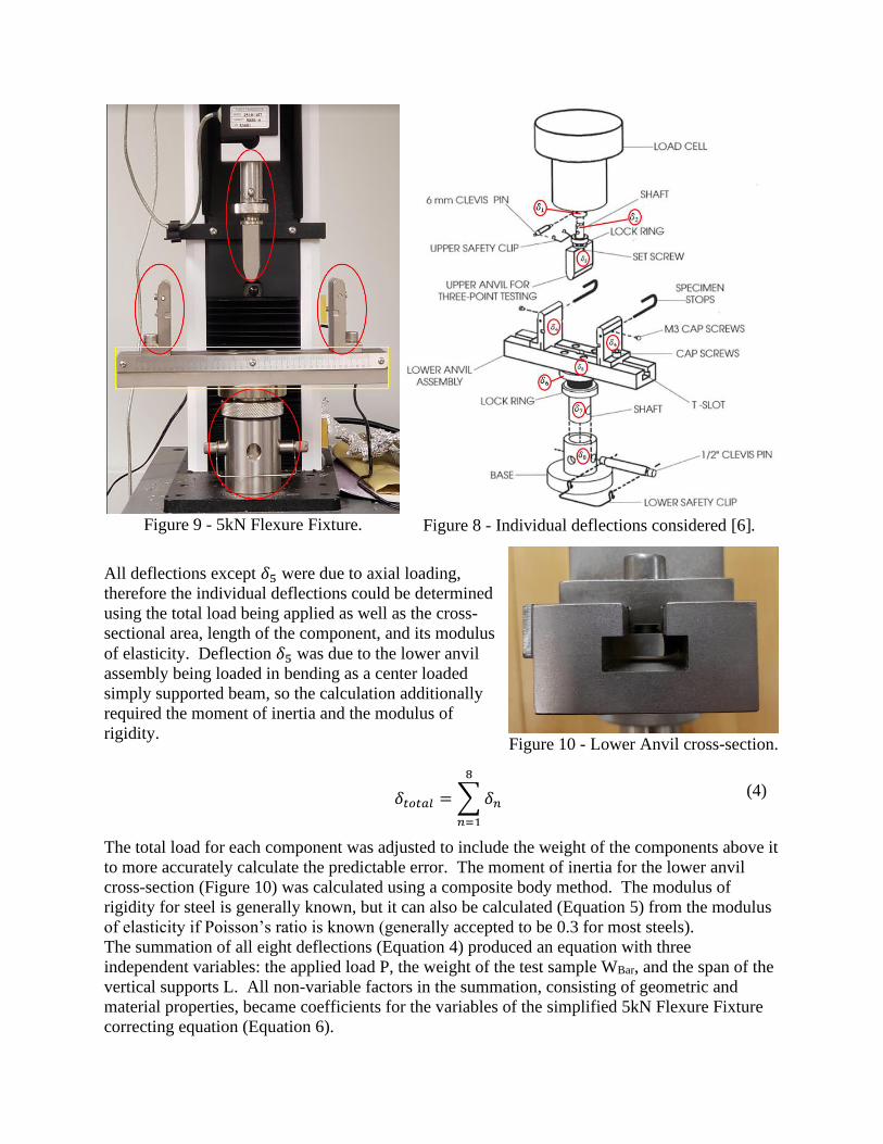
Hand calculations to determine the internal deflections within the 5kN Flexure Fixture (Figure 9)

for every component between the load cell and the Instron base plate was performed. All

components of the flexure fixture were made of steel, therefore a modulus of elasticity of 2x1011

Pascals was used for these calculations. The axially loaded member’s deflections (circled in red)

were calculated using Equation 1 while the deflection for the lower anvil assembly experiencing

bending (circled in yellow) was calculated using Equation 3. The eight individual deflections

(Figure 8) were then summed to create the deflection equation (Equation 4).

Figure 7 - Dimensions of 5kN Flexure Fixture components in millimeters.

UPPER ANVIL UPPER SHAFT

VERTICAL SUPPORTS

LOWER ANVIL ASSEMBLY

BASE ADAPTER

All deflections except 𝛿5 were due to axial loading,

therefore the individual deflections could be determined

using the total load being applied as well as the cross-

sectional area, length of the component, and its modulus

of elasticity. Deflection 𝛿5 was due to the lower anvil

assembly being loaded in bending as a center loaded

simply supported beam, so the calculation additionally

required the moment of inertia and the modulus of

rigidity.

The total load for each component was adjusted to include the weight of the components above it

to more accurately calculate the predictable error. The moment of inertia for the lower anvil

cross-section (Figure 10) was calculated using a composite body method. The modulus of

rigidity for steel is generally known, but it can also be calculated (Equation 5) from the modulus

of elasticity if Poisson’s ratio is known (generally accepted to be 0.3 for most steels).

The summation of all eight deflections (Equation 4) produced an equation with three

independent variables: the applied load P, the weight of the test sample WBar, and the span of the

vertical supports L. All non-variable factors in the summation, consisting of geometric and

material properties, became coefficients for the variables of the simplified 5kN Flexure Fixture

correcting equation (Equation 6).

𝛿𝑡𝑜𝑡𝑎𝑙 = ∑ 𝛿𝑛

8

𝑛=1

(4)

Figure 9 - 5kN Flexure Fixture.

Figure 8 - Individual deflections considered [6].

Figure 10 - Lower Anvil cross-section.

To verify this correction equation, a bar that was unlikely to bend due to a very high moment of

inertia (weighing 75.4978 N) was chosen to be the test specimen (Figure 11) for both the hand

calculation and an ANSYS Workbench analysis (Figure 12).

The force placed on the top face of the 5kN Flexure Fixture was 4000 N. Standard Earth gravity

was applied so that the weight of the bar and the individual components figured into the final

deflection solution since the correction equation considered them as well. ANSYS Mechanical

was set up to solve for two directional deformations: the y-axis for the entire body and just the

top face. The top face was where the deflection values would be comparable to the correcting

equation results. When the solution was complete, contour plots showing the directional

deformation of the body (Figure 13) and the top face (Figure 14) were produced. The result of

the comparison of the top face directional deformation with the error correction calculation was

then performed (Table 2). The maximum percent error between ANSYS and the hand

calculation values was 1.598% with the average percent error being 0.457% validating this

correction equation component.

𝐺 =

𝐸

2(1 + 𝑣)

(5)

Where:

G = the modulus of rigidity

E = the modulus of elasticity

v = Poisson’s ratio

5𝑘𝑁 𝐹𝑙𝑒𝑥𝑢𝑟𝑒 𝐹𝑖𝑥𝑡𝑢𝑟𝑒 𝐶𝑜𝑟𝑟𝑒𝑐𝑡𝑖𝑜𝑛= 1.67 ∗ 10−6𝑃𝐿3 + 1.67 ∗ 10−6𝑊𝑏𝑎𝑟𝐿3 + 1.57 ∗ 10−5𝐿3

+ 3.69 ∗ 10−9𝑃𝐿 + 3.69 ∗ 10−9𝑊𝑏𝑎𝑟𝐿 + 3.46 ∗ 10−8𝐿 + 2.98∗ 10−9𝑃 + 7.47 ∗ 10−10𝑊𝑏𝑎𝑟 + 8.87 ∗ 10−9

(6)

Figure 11 - Verification setup.

Figure 12 - ANSYS model boundary conditions.

Repeatable Errors

With the 5kN Flexure Fixture deflections accounted for, the

remaining repeatable deflections in the system needed to be

determined. An experimental setup (Figure 15) was

generated to determine the remaining system deflection.

The bar of very high moment of inertia was once again

utilized since its internal deflections due to axial loading

could be considered negligible due to its large cross-

sectional area. Due to the geometric trait that the

compression test plate’s diameter was large compared to its

Figure 15 - Experimental setup

for remaining system deflection.

Figure 16 - Remaining system deflection analysis results.

Figure 13 - Total system directional deformation.

Figure 14 - Top face directional deformation.

Table 2 - ANSYS and Hand Calculation Comparison.

height, its internal deflections could also be deemed negligible. Therefore, most of the reported

deflection should be from the remainder of the system. It was expected that the remaining

repeatable system deflection would be comprised of the deflection in the load cell and the

Instron’s column. Due to the nature of the suspected remaining deflections, it was suspected that

the results would be nonlinear, and a cubic polynomial approximation appeared to fit best. Also,

given that there should be no deflection when there was no load, a zero intercept was specified.

The resulting deflection data was processed, and a zero-intercept linear regression analysis was

performed (Figure 16) to generate the remaining system correction equation (Equation 7).

Results

With the total system deflection analysis completed, the total system correction equation

(Equation 8) was created by summing Equations 6 and 7. The impact of the test specimen’s

weight was investigated by letting Wbar = 0. Since the test specimen would not typically weigh

more than 2 N, and since doing so resulted in a difference approximately equal to 0, a simplified

total system corrections equation resulted (Equation 9).

A graphical representation of the

total system corrections equation

was generated (Figure 17) using

MATLAB to investigate the

sensitivity of the correction

equation to the different

independent variables. As

expected, the correction equation is

more sensitive to load than the span

of the vertical supports.

With the final total system

correction equation developed,

verification was sought through

experimental testing. Several

materials were selected for testing

𝑅𝑒𝑚𝑎𝑖𝑛𝑖𝑛𝑔 𝑆𝑦𝑠𝑡𝑒𝑚 𝐶𝑜𝑟𝑟𝑒𝑐𝑡𝑖𝑜𝑛 = 3.2228 ∗ 10−15𝑃3 − 2.5081 ∗ 10−11𝑃2 + 2.2097 ∗ 10−7𝑃

(7)

𝑇𝑜𝑡𝑎𝑙 𝑆𝑦𝑠𝑡𝑒𝑚 𝐶𝑜𝑟𝑟𝑒𝑐𝑡𝑖𝑜𝑛= 1.67 ∗ 10−6𝑃𝐿3 + 3.22 ∗ 10−6𝑃3 + 1.57 ∗ 10−5𝐿3 − 2.51∗ 10−11𝑃2 + 3.69 ∗ 10−9𝑃𝐿 + 3.46 ∗ 10−8𝐿 + 2.24 ∗ 10−7𝑃+ 8.87 ∗ 10−9

(9)

𝑇𝑜𝑡𝑎𝑙 𝑆𝑦𝑠𝑡𝑒𝑚 𝐶𝑜𝑟𝑟𝑒𝑐𝑡𝑖𝑜𝑛= 1.67 ∗ 10−6𝑃𝐿3 + 3.22 ∗ 10−6𝑃3 + 1.67 ∗ 10−6𝑊𝑏𝑎𝑟𝐿3

+ 1.57 ∗ 10−5𝐿3 − 2.51 ∗ 10−511𝑃2 + 3.69 ∗ 10−9𝑃𝐿 + 3.69∗ 10−9𝑊𝑏𝑎𝑟𝐿 + 3.46 ∗ 10−8𝐿 + 2.24 ∗ 10−7𝑃 + 7.47∗ 10−10𝑊𝑏𝑎𝑟 + 8.87 ∗ 10−9

(8)

Figure 17 - 3D Plot of Total System Correction Equation.

with different geometric and modulus of elasticity properties (Table 3) to be evaluated at

different vertical spans to determine how close the correction equation modified data predicted

the test specimen’s known moduli of elasticity.

The testing sequence desired was as follows:

1. Set vertical support span to 10 cm

2. Bend 9 test samples (three geometries of three materials) until yielding or 4000 N

3. Export data to correcting excel spreadsheet

4. Repeat steps 1-3 for vertical spans of 12 cm and 14 cm

Table 3 - Test Sample Geometric and Mechanical Properties.

Material Width (in) Thickness (in) Modulus of Elasticity (psi)

4140 Steel

0.25 0.25

2.97x107 [5] 0.25 0.5

0.5 0.25

6061 T6 Aluminum

0.25 0.25

1.00x107 [5] 0.25 0.5

0.5 0.25

360 HO2 Brass

0.25 0.25

1.41x107 [5] 0.25 0.5

0.5 0.25

Table 4 - Modulus of elasticity verification test results.

Two of the material/geometry combinations did not yield useable results. The 0.25 x 0.5 4140

steel specimens were too stiff to give useable results. In retrospect, milder steel should have

been chosen so that useable results could have been obtained from this geometry. The 0.25 x

0.25 360 H02 brass specimens did not appear to be the same material as the other two brass

geometries since the modulus of elasticity was half that of the others and none were close to

what was expected from the specific material ordered. This was possibly due to a quality control

issue. These values were all reported as N/A in the verification of test results (Table 4).

The percent error improved by 13.98% (on average from an original percent error of 23.21% to a

corrected percent error of 9.92%). The percent difference improved by 17.02% (on average from

an original percent difference of 27.79% to a corrected percent difference of 10.77%). Overall, a

reasonable improvement. If one were to discount the brass tests (due to suspected quality control

issues regarding the material received), the percent error improvement would be 11.8% (on

average from an original percent error of 16.40% to a corrected percent error of 4.62%) and the

percent difference improved by 13.99% (on average from an original percent difference of

18.55% to a corrected percent difference of 4.56%). Much better results, as the remaining errors

were under 5%.

Several other observations were obtained from the results of this verification testing. The first

being that the Load–Deflection curves (Figure 18) showed linear segments whose slopes were

the spring constant (k) for that material and geometry combination. Each of the three test

specimens for this material and span showed different k values because they had different

stiffnesses. Second, the stiffer the specimen, the more error there was to be corrected.

Next, the corrected curves show a higher

modulus of elasticity (slope) and lay close to

each other (Figure 19). The uncorrected

curves show that the stiffer the specimen, the

lower the slope value. Only the linear portion

of the curves from the load-deflection results

was used for this graph. Note: the horizontal

axis represents the deflection modified by a

constant determined by Equation 10 and has

the units of in2, which when combined with

the vertical axis units of lbf, results in the

slope of the curves having the units of psi, for

modulus of elasticity.

Lastly, with the material and specimen

geometry held constant, the effect of the span

could be observed (Figure 20). As with the

previous results, the corrected curves were

very close to each other. The remaining

𝐴𝑑𝑗𝑢𝑠𝑡𝑒𝑑 𝐷𝑒𝑓𝑙𝑒𝑐𝑡𝑖𝑜𝑛 = 𝛿 ∗

48 ∗ 𝐼

𝐿3 (10)

Figure 18 – Load-deflection curves.

curves had a slope whose values became lower as their span decreased. This was to be expected

since the specimen becomes harder to bend and thus behaved as if it was stiffer.

Figure 19 - Modulus of elasticity slopes (original and corrected).

Figure 20 - Modulus of elasticity slopes (original and corrected) for various spans.

Discussion

This verification process showed that an error still existed between theoretical and experimental

modulus of elasticity values. This trait of the data was noted but no additional correction was

applied to further address the remaining discrepancies. The reasoning behind this decision was

that if all the error was accounted for, the students would have no error analysis section in their

lab reports. The originally identified purpose of the developed correction equation was to correct

most of the errors in the testing system (the predictable and repeatable errors, specifically).

Therefore, the ability of the student to correctly determine the unknown material used during

testing would be substantially improved using this correcting equation. The minor error

remaining could be due to errors in the load cell, the weight of the specimen, variation in the

specimen’s length during deflection, and others. It remains for the student to acknowledge the

existence of these minor errors and report them in their findings along with their reasoning

behind the differences between theoretical and measured modulus of elasticity values.

Conclusions

A correction equation was found that reduced errors existing in testing data from an Instron 3345

Single Column Universal Testing System with a 5 kN Static 3 Point Flexure Fixture to under

5%. This allows the student to more accurately determine the modulus of elasticity and, thus,

determine the material (or its alloy) being tested. Introducing this type of experiment to the

engineering mechanics curriculum would enhance a student’s ability to obtain the course

objectives by allowing them to demonstrate their level of knowledge of the strengths of

materials.

References

[1] K. Mobley and S. Fisher, "Ditching the Desks: Kinesthetic Learning in College

Classrooms," The Social Studies, vol. 105, no. 6, pp. 301-309, 2014.

[2] R. C. Hibbeler, Statics & Mechanics of Materials, 4th ed., Upper Saddle River, New Jersey:

Pearson, 2014.

[3] M. P. Groover, Fundamentals of Modern Manufacturing, 2nd ed., New York, New York:

John Wiley & Sons, 2002.

[4] R. C. Juvinall and K. M. Marshek, Fundamentals of Machine Component Design, 5th ed.,

Hoboken, New Jersey: John Wiley & Sons, 2012.

[5] "MatWeb Material Property Data," MatWeb, [Online]. Available:

http://www.matweb.com/search/search.aspx. [Accessed 16 2 2020].

[6] Instron, TS M10-82810-11 Reference Manual, Canton, Massachusetts: Worldwide

Headquarters, 2017.