50
Synthesis Techniques Juan P Bello

Synthesis Techniques
Juan P Bello

Synthesis• It implies the artificial construction of a complex body by
combining its elements. Complex body: acoustic signal (sound) Elements: parameters and/or “basic signals”
• Motivations: Reproduce existing sounds Reproduce the physical process of sound generation Generate new pleasant sounds Control/explore timbre
Model / representation Sound
Synthesis

• Oscillators are used to generate a raw repeating signal/waveform.
Oscillators
oscAmplitude
FrequencyOutput signal
Wavetable

Oscillators• Can use any waveform stored in a memory list (wavetable)
• Called back whenever necessary (table look-up)• Repetitive scanning (at a variable phase increment) produces a
pitched sound
Over-sampling and interpolation are combined to maximise its use
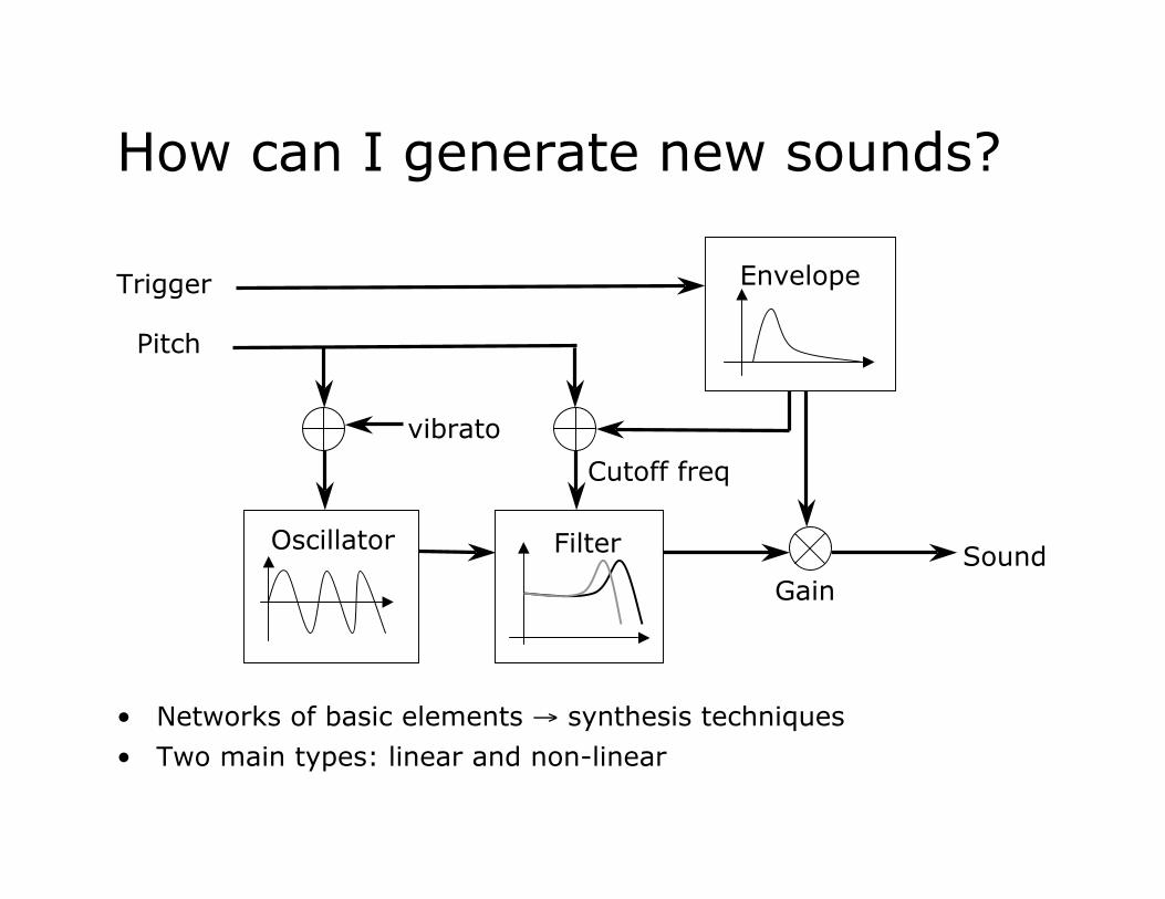
How can I generate new sounds?
FilterOscillator
Envelope
vibrato
Pitch
Trigger
Cutoff freq
GainSound
• Networks of basic elements → synthesis techniques
• Two main types: linear and non-linear

Additive Synthesis• It is based on the idea that complex waveforms can be created by
the addition of simpler ones.• It is a linear technique, i.e. do not create frequency components
that were not explicitly contained in the original waveforms• Commonly, these simpler signals are sinusoids (sines or cosines)
with time-varying parameters, according to Fourier’s theory:
( )!=
+=0
2sin)(i
iii tfAts "#
Amp1(t)Freq1(t)
Amp2(t)Freq2(t)
AmpN(t)FreqN(t)
Σ

Additive Synthesis:
A Pipe Organ

Additive Synthesis• Square wave: only odd harmonics. Amplitude of the nth harmonic= 1/n

Time-varying sounds
AmpFreq
Amp1(t)
Freq1(t)
AmpFreq
Amp2(t)
Freq2(t)
AmpFreq
AmpN(t)
FreqN(t)
Σ
• According to Fourier, all sounds can be described and reproducedwith additive synthesis.
• Even impulse-like components can be represented by using ashort-lived sinusoid with “infinite” amplitude.
• Additive synthesis is very general (perhaps the most versatile).• Control data hungry: large number of parameters are required to
reproduce realistic sounds

Analysis/Resynthesis
• Different techniques that employ a lossy parameterisation of asound to facilitate its manipulation and reproduction
• The concept applies to additive synthesis, subtractive synthesis,combinations of the two, etc.
• Examples include the phase-vocoder and sinusoidal modelling
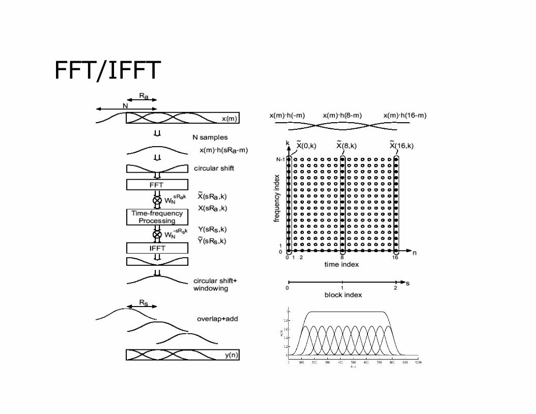
FFT/IFFT

Sinusoidal + Noise model (1)
Sinusoidal modellingsignal
Residual(mostly transients)
Tonal part
-

Sinusoidal + Noise model (2)

• Filtering with arbitrary resolution
• Partial dependant frequency scaling
SMS Transformations
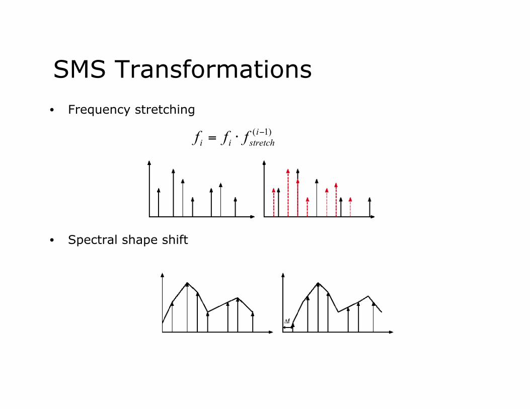
• Frequency stretching
• Spectral shape shift
SMS Transformations
)1( !"=
i
stretchii fff

Examples
water
guitar
flute
transSMSstochdetorig

SMS Effects
• Content-dependent processing, e.g. real-time singing voiceconversion (vocaloid)

Summary: additive synthesis• Probably the most versatile synthesis method as any sound (old or
new) can be represented
• Unusually accurate: even small variations can be reproduced
• Too much control data, and only changes in large amounts of thisdata bring perceptually-relevant sound modifications
• Thus, requires the use of analysis/resynthesis methodologies (e.g.phase vocoder, SMS, etc) to simplify control
• It is not well suited to deal with stochastic (impulse-like)components and highly transient signals

• Is another linear technique based on the idea that sounds can begenerated from subtracting (filtering out) components from a veryrich signal (e.g. noise, square wave).
• Its simplicity made it very popular for the designof analog synthesisers (e.g. Moog)
Subtractive Synthesis
fA Sound
GainParameters
ComplexWaveform Filter Amplifier

The human speech system• The vocal chords act as an oscillator, the mouth/nose cavities,
tongue and throat as filters• We can shape a tonal sound (‘oooh’ vs ‘aaah’), we can whiten the
signal (‘sssshhh’), we can produce pink noise by removing highfrequencies

Source-Filter model• Subtractive synthesis can be seen as a excitation-resonator or
source-filter model• The resonator or filter shapes the spectrum, i.e. defines the spectral
envelope

What is the spectral envelope?
• It is a smoothing of the spectrum that preserves its general formwhile neglecting its spectral line structure

Source-Filter model
Envelope estimation
Whitening of the signal Transformations
Analysis Processing Synthesis
!=
"=
p
k
k
k zazP1
)(
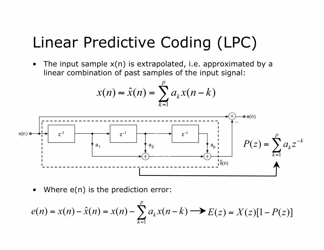
Linear Predictive Coding (LPC)• The input sample x(n) is extrapolated, i.e. approximated by a
linear combination of past samples of the input signal:
• Where e(n) is the prediction error:
!=
"=#p
k
k knxanxnx1
)()(ˆ)(
!=
""="=p
k
k knxanxnxnxne1
)()()(ˆ)()( )](1)[()( zPzXzE !=

Linear Predictive Coding (LPC)• For synthesis, we just inverse the process :
• H(z) is an IIR filter known as the LPC filter which represents thespectral model of x(n).
H(z))(1
)(zP
GzH
!=

Linear Predictive Coding (LPC)• With optimal coefficients -> prediction error energy is minimised• The higher the coefficient order p, the closer the approximation is
to |X(k)|
• Thus the problem of linear prediction becomes the estimation ofthe set of coefficients ak from the input signal x(n).
• This can be efficiently solved using the Yule-Walker equations

Summary: subtractive synthesis• Low-order filtering is very intuitive, hence easy to use.
• Most parameters directly map to psychophysical concepts (e.g. thefrequency of the oscillator to pitch, the filter shaping to timbre).
• Our ears are used to sounds generated following these principlesas this is the working principle of speech.
• That also impose limitations on the versatility of the approach.
• As in additive synthesis it requires the use of analysis-resynthesistechniques to control accurate sound simulations using a fewparameters.

Amplitude modulation• Non-linear technique, i.e. results on the creation of frequencies
which are not produced by the oscillators.• In AM the amplitude of the carrier wave is varied in direct
proportion to that of a modulating signal.
Ampm(t)
Freqm(t)
Ampc(t)
Freqc(t)
modulator carrier
bipolar unipolar
Bipolar -> Ring modulationUnipolar -> Amplitudemodulation

• Let us define the carrier signal as:
• And the (bipolar) modulator signal as:
• The Ring modulated signal can be expressed as:
• Which can be re-written as:
• s(t) presents two sidebands at frequencies: ωc - ωm and ωc + ωm
Ring Modulation
)cos()( tAtccc
!=
)cos()( tAtmmm
!=
( ) ( )tAtAtsmmcc
!! coscos)( "=
[ ]( ) [ ]( )[ ]ttAA
tsmcmc
mc !!!! ++"= coscos2
)(

Ring Modulation
freq
amp
fc
fc - fm fc + fm

Single-sideband modulation
m(t)
!"#
<+
>$=
0
0)(
%
%%
j
jjH
sinωct
cosωct
s(t)
|H(jω)|
ω
1
∠H(jω)
ω
π/2
-π/2
90° phase-shifts1(t)
s2(t)

Single-sideband modulationM(ω)
ω
1
S1(ω)
ω
--1/2
ωc-ωc
S2(ω)
ω
--1/2
ωc-ωc
S (ω)
ω
--1
ωc-ωc
With changes of ωc the spectrumof m(t) will be shifted accordingly,so SSB modulation is also knownas frequency shifting

• Let us define the carrier signal as:
• And the (unipolar) modulator signal as:
• The amplitude modulated signal can be expressed as:
• Which can be re-written as:
• s(t) presents components at frequencies: ωc , ωc - ωm and ωc + ωm
Amplitude Modulation
)cos()( ttcc
!=
)cos()( tAAtmmmc
!+=
( )[ ] ( )ttAAtscmmc
!! coscos)( +=
( ) [ ]( ) [ ]( )[ ]ttA
tAtsmcmc
m
cc!!!!! ++"+= coscos
2cos)(

Modulation index• In modulation techniques a modulation index is usually defined such
that it indicates how much the modulated variable varies around itsoriginal value.
• For AM this quantity is also known as modulation depth:
c
m
A
A=!
• If β = 0.5 then thecarrier’s amplitudevaries by 50% aroundits unmodulated level.
• For β = 1 it varies by100%.
• β > 1 causes distortionand is usually avoided

C/M frequency ratio
• Lets define the carrier to modulator frequency ratio c/m (= ωc /ωm) for a pitched signal m(t)
• If c/m is an integer n, then ωc, and all present frequencies, aremultiples of ωm (which will become the fundamental)
• If c/m = 1/n, then ωc will be the fundamental
• When c/m deviates from n or 1/n (or more generally, from aratio of integers), then the output frequencies becomes moreinharmonic
• Example of C/M frequency variation

Summary: AM synthesis• Easy to implement and extremely low computational cost
• A few parameters with direct control on the sonic output: Amaffects the depth of change of Ac (modulation depth), fm affectsthe rate of change of Ac and c/m determines the perceivedfrequency of the sound
• Requires caution: fc+fm exceeding fs/2 causes aliasing, whilesmall fc-fm may not be audible or cause inharmonicity
• Little possibilities given the simplicity of the method (not enoughspectral complexity to synthesise rich timbres)

Frequency Modulation• Frequency modulation (FM) is a form of modulation in which the
frequency of a carrier wave is varied in direct proportion to theamplitude variation of a modulating signal.
• When the frequency modulation produces a variation of lessthan 20Hz this results on a vibrato.
Ampm(t)
Freqm(t)
Ampc(t)
Freqc(t)
modulator carrier
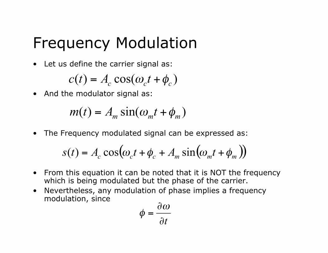
• Let us define the carrier signal as:
• And the modulator signal as:
• The Frequency modulated signal can be expressed as:
• From this equation it can be noted that it is NOT the frequencywhich is being modulated but the phase of the carrier.
• Nevertheless, any modulation of phase implies a frequencymodulation, since
Frequency Modulation
)cos()(ccc
tAtc !" +=
)sin()(mmm
tAtm !" +=
( )( )mmmccc
tAtAts !"!" +++= sincos)(
t!
!=
"#

• Let us re-write the expression of the modulated signal as:
• Where Ac = 1, φc = φm = 0 and Am is renamed β for simplicity. Usingphasor analysis and the 2-sided Laurent expansion:
• we can derive the expression:
• Where Jk(β) are known as the Bessel functions of the first kind, k istheir integer order and β is the argument. Jk(β) is real, and J-k(β) =(-1)kJk(β).
Frequency Modulation
( )( )tttsmc
!"! sincos)( +=
( )[ ]!"
#"=
+=k
mcktkJts $$% cos)()(
!"
#"=
=k
tjk
k
tj mm eJe$$% % )()sin(

• If β ≠ 0 then the FM spectrum contains infinite sidebands atpositions ωc± kωm.
Frequency Modulation
β k
Jk
• The amplitudes of each pair ofsidebands are given by the Jkcoefficients which are functionsof β

Modulation index
• As in AM we define a FM modulation index that controls themodulation depth.
• In FM synthesis this index is equal to β, the amplitude of themodulator and is directly proportional to Δf.
• As we have seen the value of β determines the amplitude of thesidebands of the FM spectrum
• Furthermore the amplitude decreases with the order k.• Thus, although theoretically the number of sidebands is infinite, in
practice their amplitude makes them inaudible for higher orders.• The number of audible sidebands is a function of β, and is
approximated by 2β+1• Thus the bandwidth increases with the amplitude of m(t), like in
some real instruments

C/M frequency ratio• The ratio between the carrier and modulator frequencies c/m
is relevant to define the (in)harmonic characteristic of s(t).
• The sound is pitched (harmonic) if c/m is a ratio of positiveintegers: ωc / ωm = Nc / Nm
• E.g. for fc = 800 Hz and fm = 200 Hz, we have sidebands at600Hz and 1kHz, 400Hz and 1.2kHz, 200Hz and 1.4kHz, etc
• Thus the fundamental frequency of the harmonic spectrumresponds to: f0 = fc / Nc = fm / Nm
• If c/m is not rational an inharmonic spectrum is produced
• If f0 is below the auditory range, the sound will not beperceived as having definitive pitch.

Sideband reflection
• For certain values of the c/m ratio and the FM index β,extreme sidebands will reflect into the audible spectrum(aliasing)
• The modulation may generate negative frequencies.Depending on the phase of the carrier and the modulator, wemight end up with an expansion containing only sines.
• As: sin(-α) = -sin(α), the lower sidebands might reflect backinto the spectrum in 180-degree phase inverted form: a halfcycle (π) phase shift implying negative amplitude.
• These reflected sidebands could add richness to the spectrum• Also they could cancel out components if they overlap exactly
with positive components.

FM examples

Summary: FM synthesis• Cost efficient and easy to implement
• Due to a strong mathematical formulation, the effects of parameterchange are, in a sense, easy to predict.
• c/m determines the location of frequency components and βdetermines their amplitude prominence
• It is well-suited for original synthesis
• The synthesis procedure bears no resemblance to the formation ofsound in nature. Hence, the method is poorly suited to simulationof acoustical instruments
• It has a distinctive sound which is difficult to escape (an possiblyannoying in the long run) mostly due to the symmetric spectrum

• Also known as non-linear distortion• It is a synthesis method where the sound signal is passed through
a function (a distortion box), such that the function w maps anyinput value x in [-1,1] to an output value w(x) in the same range.
• W is the shaping function.
• The value of A is of great importance as the scaling of the inputsignal makes it reference to different regions of W.
Waveshaping synthesis
ω
A
Wx W(x)
x

• If W is a straight diagonal line from -1 to 1, then the process islinear, otherwise x is distorted by W.
Waveshaping synthesis

• Waveshaping is amplitude sensitive.• This is useful to simulate the behaviour of acoustic instruments’
sounds: the harder an instrument is played the richer its spectrum• An input signal with time-varying amplitude, produces an output
whose spectrum changes according to that variation.• A variation in the time-domain is translated into a variation in the
frequency domain.• Thus, waveshaping produces a variety of waveforms with simple
amplitude variations at the input (very efficient).
Waveshaping synthesis
-1 1-1
1

• LeBrun (1979) and Arfib (1979) demonstrated that it is possibleto predict the output spectrum of the waveshaped signal if x is acosine wave and W belongs to the Chebyshev family ofpolynomials
• The kth Chebyshev polynomial of the first kind Tk is definedthrough the identity:
• Thus, if we apply the kth Chebyshev polynomial to a sinusoid weobtain a cosine wave at the kth harmonic.
• Each Chebyshev polynomial, when used as W, produces aparticular harmonic of x.
• A weighted combination of Chebyshev polynomials as W, willproduce a corresponding harmonic mixture, E.g.:
Chebyshev functions
)cos()cos( !! kTk
=
42025.05.0 TTT ++

Closing remarks
Modulation methodsModulation methods
Subtractive synthesisSubtractive synthesis
Additive SynthesisAdditive Synthesis
IncreasinglyIncreasingly General General
Fewer ControlFewer Control Parameters Parameters


