Synthesising Model Projections of Future Climate ChangeMat Collins, Exeter Climate Systems, College of Engineering, Mathematics and Physical Sciences, University of Exeter and Met Office Hadley Centre

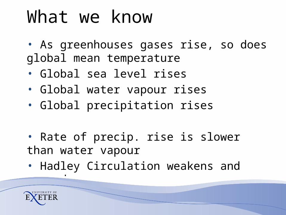
What we know

• As greenhouses gases rise, so does global mean temperature• Global sea level rises• Global water vapour rises• Global precipitation rises

• Rate of precip. rise is slower than water vapour• Hadley Circulation weakens and expands• …

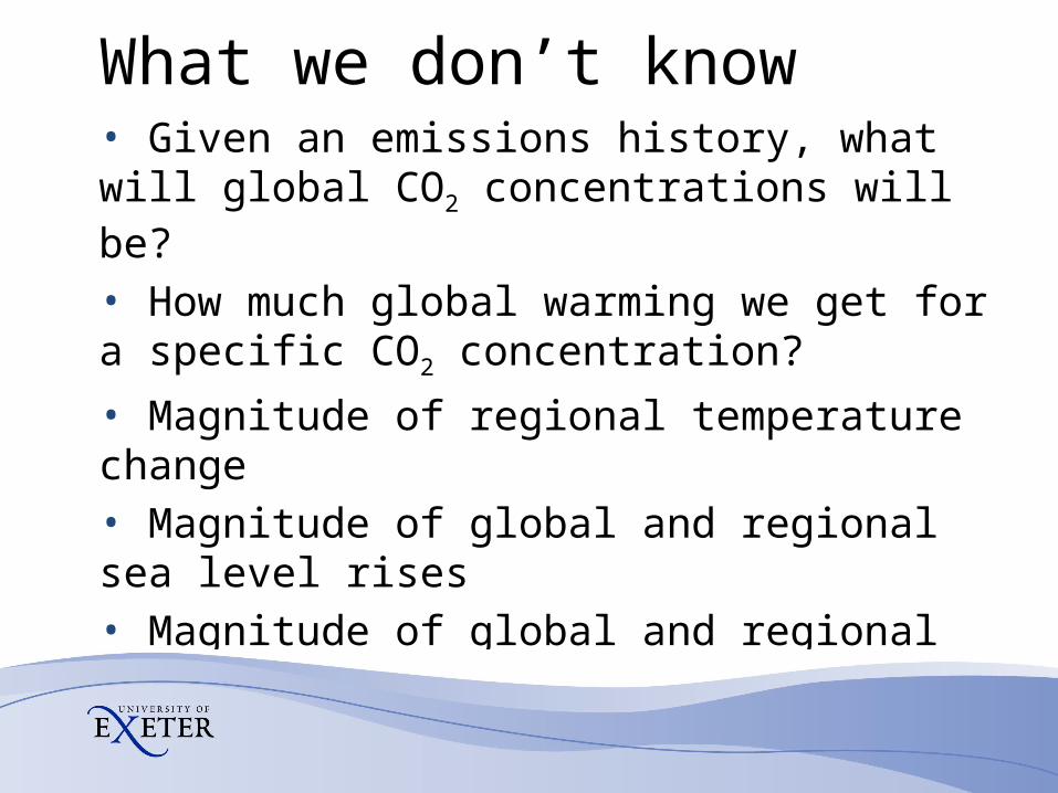
What we don’t know• Given an emissions history, what will global CO2 concentrations will be?

• How much global warming we get for a specific CO2 concentration?

• Magnitude of regional temperature change• Magnitude of global and regional sea level rises• Magnitude of global and regional precipitation change• …

© Crown copyright Met Office

• The Coupled Model Intercomparison Project (CMIP) collects output from the climate models from all over the world and provide web access• This has become the “gold standard” in assessing uncertainties in projections• CMIP5 will produce 2.3 Pb data*• However, should all models be treated as equally likely?• Is the sample somehow representative of the “true” uncertainty?• Could there be surprises and unknown unknowns?

Models, models, models

* 25 years to download on home broadband link, Internet archive = 3Pb, LHC will produce 15 Pb of data, World of Warcraft = 1.3 Pb (source Wikipedia).

Figure 8.5

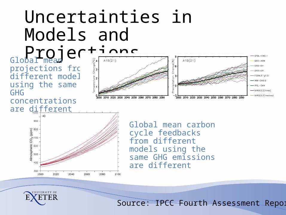
Uncertainties in Models and Projections

Source: IPCC Fourth Assessment Report

• Models have “errors” i.e. when simulating present-day climate and climate change, there is a mismatch between the model and the observations

• Differences in model formulation can lead to differences in climate change feedbacks

• Cannot post-process projections to correct errors

Figure 10.20

Uncertainties in Models and Projections

Global mean projections from different models using the same GHG concentrations are different

Figure 10.5

Global mean carbon cycle feedbacks from different models using the same GHG emissions are different

Source: IPCC Fourth Assessment Report

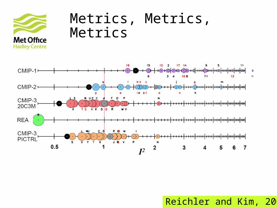
Metrics, Metrics, Metrics

Reichler and Kim, 2008

Techniques for Projections(projection = dependent on emissions scenario)

• Extrapolation of signals (e.g. ASK)• The meaning of simple ensemble averaging• Emergent constraints• Single-model Bayesian approaches (including “objective” Bayes)• Challenges

© Crown copyright Met Office

Robust quantification of contributors to past temperature change enables quantification of likely future rates of warming (ASK)

Global mean NH - SH

Land - ocean MTG

© Crown copyright Met Office

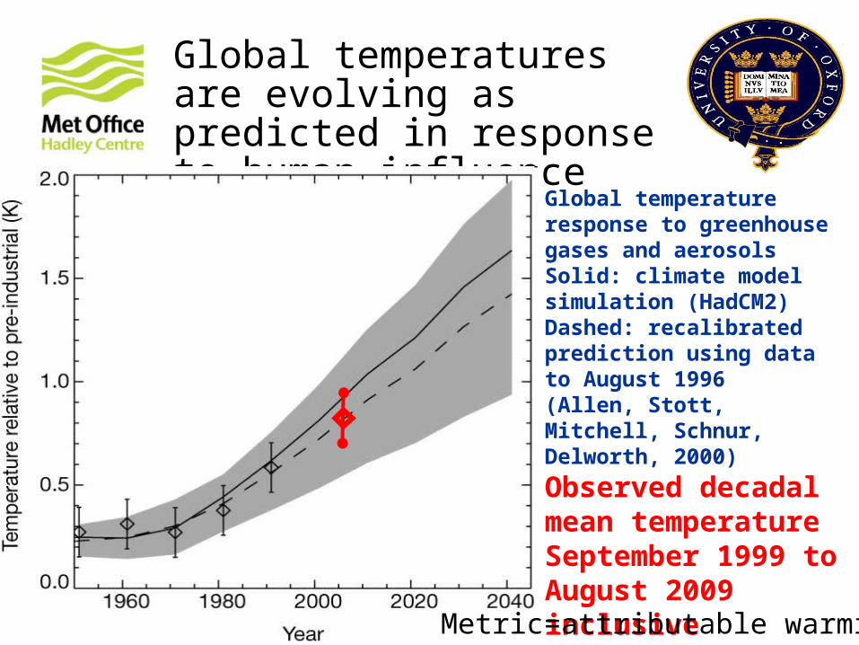
Global temperatures are evolving as predicted in response to human influence

Global temperature response to greenhouse gases and aerosolsSolid: climate model simulation (HadCM2)Dashed: recalibrated prediction using data to August 1996(Allen, Stott, Mitchell, Schnur, Delworth, 2000)

Observed decadal mean temperature September 1999 to August 2009 inclusive

Metric=attributable warming

What about regional information?

Figure 10.9

Source: IPCC Fourth Assessment Report

How do we interpret the ensemble mean and spread?

Rank histograms from CMIP3 output

Loop over grid points and rank the observation w.r.t. ensemble members, compute histogram

Uniform histogram is desirable

U-shaped = too narrow

Domed = too wide

Tokuta Yokohata, James D. Annan, Julia C. Hargreaves, Charles S. Jackson, Michael Tobis, Mark J. Webb, David Sexton, Mat Collins

Emergent Constraints: Schematic

• Find relationship• Find observed value• Read off prediction• Find observational

uncertainty• Add onto prediction• Add “statistical” uncertainty

from scatter

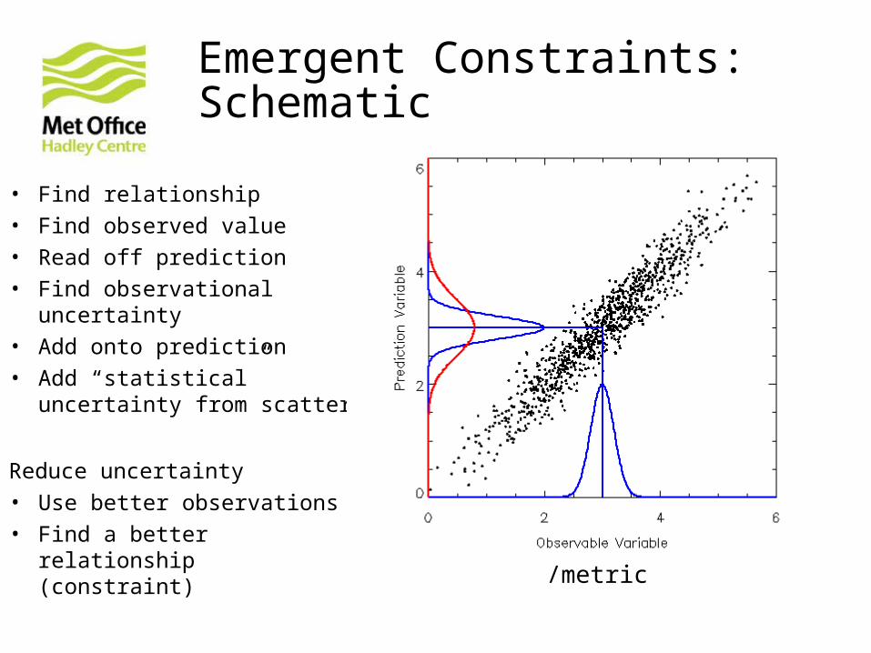
Reduce uncertainty• Use better observations• Find a better relationship

(constraint)/metric

• Boé J, Hall A, Qu X (2009), September Sea-Ice Cover in the Arctic Ocean Projected to Vanish by 2100, Nature Geosci, 2: 341-343

• Hall A, Qu X (2006) Using the current seasonal cycle to constrain snow albedo feedback in future climate change. Geophys. Res. Lett., 33, L03502

Emergent Constraints

PalaeoQUMP: QUEST Project

• Tamsin Edwards, Sandy Harrison, Jonty Rougier, Michel Crucifix, Ben Booth, Philip Brohan, Ana María García Suárez, Mary Edwards, Michelle Felton, Heather Binney, …

• Aim: To use palaeoclimate data and simulations to constrain future projections

Feedback parameter (climate sensitivity) vs different metrics

Single Model Bayesian Approches: The Perturbed Physics Ensemble

• Take one model structure and perturb uncertain parameters and possible switch in/out different subroutines

• Can control experimental design, systematically explore and isolate uncertainties from different components

• Potential for many more ensemble members

• Unable to fully explore “structural” uncertainties

• HadCM3 widely used (MOHC and climateprediction.net) but other modelling groups are dipping their toes in the water

Some Notation

y = {yh,yf} historical and future climate variables (many)

f = model (complex)

x = uncertain model input parameters (many)

o = observations (many, incomplete)

• Our task is to explore f(x) in order to find y which will be closest to what will be observed in the past and the future (conditional on some assumptions)

• Provide probabilities which measure how strongly different outcomes for climate change are supported by current evidence; models, observations and understanding

f(x)y

Probabilistic Approach

f(x)}y,{y fh

x yh

yf

input space

historical/observable climate

future climate

of(x1)

f(x1)

f(x2)

f(x2)

x1

x2

)|(o)(o)|( ypypyp

x

© Crown copyright Met Office

Emulator Schematic

• Use regression trained on ensemble runs to estimate past and future variables, {yh,yf} at any point of parameter space, x

• Use transformed variables and take into account some non-linear interaction terms

• Note – might need to run models at some quite “remote” regions of parameter space

• Keep account of emulator errors in the final PDFs

e.g. Rougier et al., 2009

Estimating Likelihood

V = obs uncertainty + emulator error

(yh-o)

(yh -o)

log L0(x) ~

V is calculated from the perturbed physics and multi-model ensembleIt is a very complicated metric

V-1

+ discrepancy

o)(yo)(y2

1||log

2(x)log h

1h0 VV Tn

cL

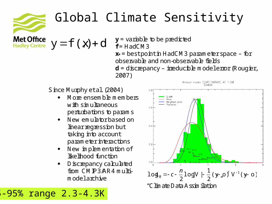
Enhancement of “Standard” Approach (Rougier 2007)

y = {yh,yf} climate variables (vector)

f = HadCM3

x* = best point in HadCM3 parameter space – for observable and non-observable fields

d = discrepancy – irreducible/”structural” model error (vector)

d)f(xy *

Estimating Discrepancy

• Use the multi-model ensemble from IPCC AR4 (CMIP3) and CFMIP (models from different centres)

• For each multi-model ensemble member, find point in HadCM3 parameter space that is closest to that member

• There is a distance between climates of this multi-model ensemble member and this point in parameter space i.e. effect of processes not explored by perturbed physics ensemble

• Pool these distances over all multi-model ensemble members

• Uses model data from the past and the future

© Crown copyright Met Office

Global Climate Sensitivity

d)f(xy * y = variable to be predicted f = HadCM3 x* = best point in HadCM3 parameter space – for observable and non-observable fields d = discrepancy – irreducible model error (Rougier, 2007)

Since Murphy et al. (2004)

More ensemble members with simultaneous perturbations to params

New emulator based on linear regression but taking into account parameter interactions

New implementation of likelihood function

Discrepancy calculated from CMIP3/AR4 multi-model archive

o)(yVo)(y2

1|V|log

2log h

1h0 Tn

cL

“Climate Data Assimilation” 5-95% range 2.3-4.3K

Page 26

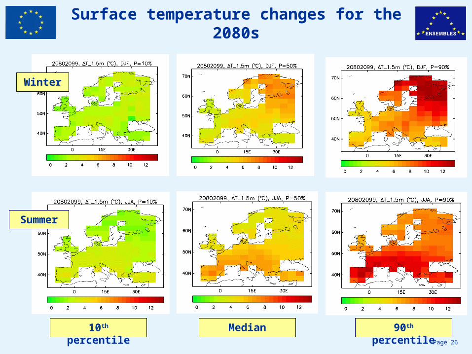
Surface temperature changes for the 2080s

10th percentile 90th percentileMedian

Winter

Summer

Page 27

Probabilistic projections in response to A1B emissions

Changes in temperature and precipitation for future 20 year periods, relative to 1961-90, at 300km scale.

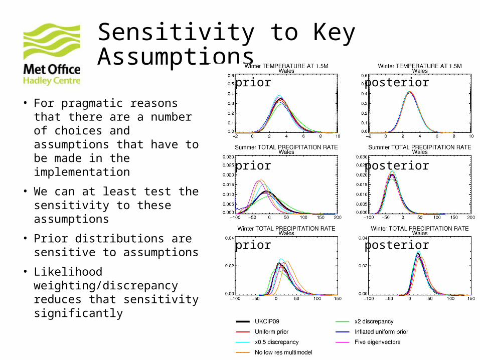
Sensitivity to Key Assumptions

• For pragmatic reasons that there are a number of choices and assumptions that have to be made in the implementation

• We can at least test the sensitivity to these assumptions

• Prior distributions are sensitive to assumptions

• Likelihood weighting/discrepancy reduces that sensitivity significantly

prior

prior

prior

posterior

posterior

posterior

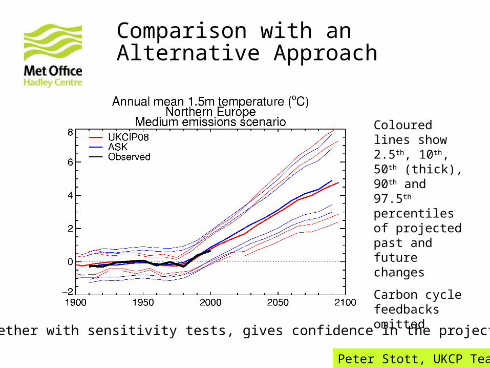
Comparison with an Alternative Approach

Coloured lines show 2.5th, 10th, 50th (thick), 90th and 97.5th percentiles of projected past and future changes

Carbon cycle feedbacks omitted

Together with sensitivity tests, gives confidence in the projections

Peter Stott, UKCP Team

Oxford University

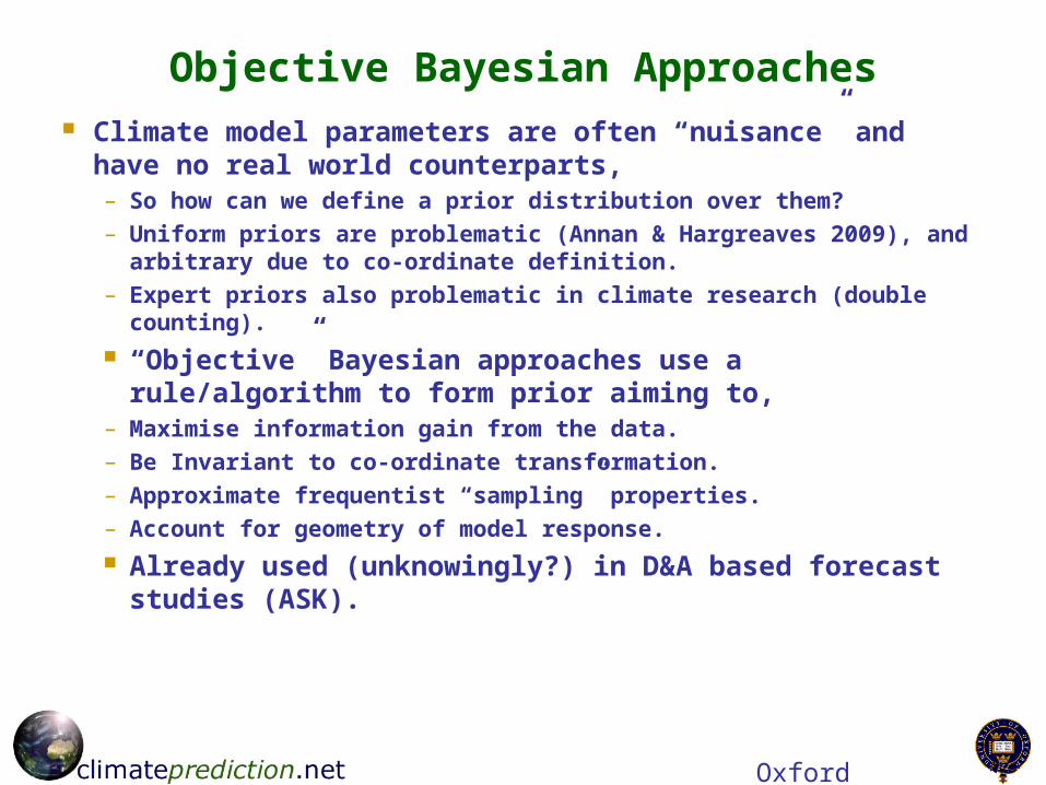
Objective Bayesian Approaches Climate model parameters are often “nuisance” and have no

real world counterparts,– So how can we define a prior distribution over them?– Uniform priors are problematic (Annan & Hargreaves 2009), and

arbitrary due to co-ordinate definition.– Expert priors also problematic in climate research (double counting).

“Objective” Bayesian approaches use a rule/algorithm to form prior aiming to,

– Maximise information gain from the data.– Be Invariant to co-ordinate transformation.– Approximate frequentist “sampling” properties.– Account for geometry of model response.

Already used (unknowingly?) in D&A based forecast studies (ASK).

Oxford University

EBM example (Rowlands 2010 in prep)

Jeffreys’ prior is the simplest approach (reference priors for the statistics aficionados).

Gives 5-95% credible interval of 2.0-4.9 K for CS. Approximately matches likelihood profile.

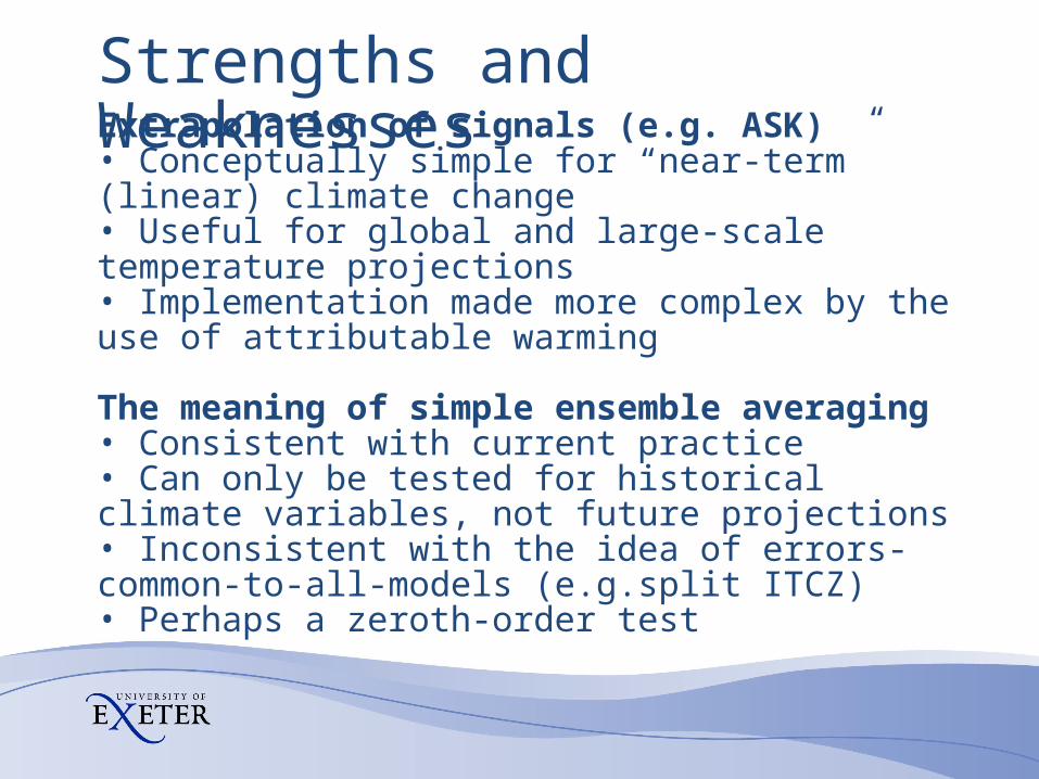
Strengths and WeaknessesExtrapolation of signals (e.g. ASK)• Conceptually simple for “near-term” (linear) climate change• Useful for global and large-scale temperature projections• Implementation made more complex by the use of attributable warming The meaning of simple ensemble averaging• Consistent with current practice • Can only be tested for historical climate variables, not future projections• Inconsistent with the idea of errors-common-to-all-models (e.g.split ITCZ)• Perhaps a zeroth-order test

Strengths and WeaknessesEmergent constraints• Strength in simplicity• Will not work for all variables (e.g. climate sensitivity)• Consistency of projections of different variables? Single-model Bayesian approaches (including “objective” Bayes)• Rigorous statistical approach• Can be implemented for “exotic” variables• Weak observational constrains • Estimating discrepancy

Challenges• Technique to produce robust, transparent, quantitative, multivariate, self-consistent projections, combining information from understanding, models and observations, agreed on by everyone

• Quantitative techniques to use metrics to improve climate models (like data assimilation in weather forecasting)• Techniques for relating present day metrics to projection skill that produce self-consistent projections of many variables

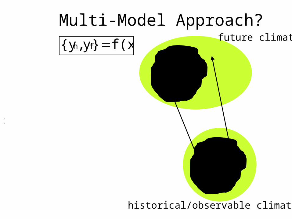
Multi-Model Approach?

f(x)}y,{y fh

x yh

yf

input space

historical/observable climate

future climate

o

Systematic Errors in All Models

Collins et al. 2010

Bayesian Approach

• Vary uncertainty model input parameters x (prior distribution of y)• Compare model output, m (‘internal’ model variables) with

observations, o, to estimate the skill of each model version (likelihood)

• Form distribution of y weighted by likelihood (posterior)

Bayesian Notation:

the posterior is proportional to the prior times the likelihood

Likelihood:

)|(o)(o)|( ypypyp

)()|(o 0 yLyp

o)g(mlog 0 L o))exp(g(m/1 w

,

,

f(x)y