Synthetic Aperture Radar Polarimetric Tomography Practical session Stefano Tebaldini Dipartimento di Elettronica, Informazione e Bioingegneria – Politecnico di Milano 5 th Advanced Training Course in Land Remote Sensing
Transcript
Synthetic Aperture Radar Polarimetric Tomography
Practical session Stefano Tebaldini
Dipartimento di Elettronica, Informazione e Bioingegneria – Politecnico di Milano
5th Advanced Training Course in Land Remote Sensing
5th Advanced Training Course in Land Remote Sensing
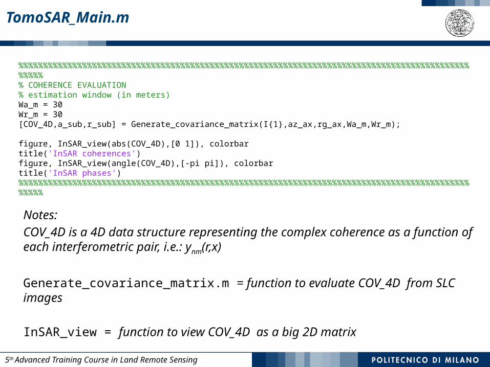
TomoSAR_Main.m
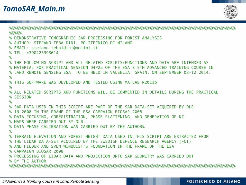
%%%%%%%%%%%%%%%%%%%%%%%%%%%%%%%%%%%%%%%%%%%%%%%%%%%%%%%%%%%%%%%%%%%%%%%%%%%%%%%%%%%%%%%%%%%%%%%%%% DEMONSTRATIVE TOMOGRAPHIC SAR PROCESSING FOR FOREST ANALYSIS% AUTHOR: STEFANO TEBALDINI, POLITECNICO DI MILANO% EMAIL: [email protected]% TEL: +390223993614%% THE FOLLOWING SCRIPT AND ALL RELATED SCRIPTS/FUNCTIONS AND DATA ARE INTENDED AS% MATERIAL FOR PRACTICAL SESSION D4P2a OF THE ESA'S 5TH ADVANCED TRAINING COURSE IN% LAND REMOTE SENSING ESA, TO BE HELD IN VALENCIA, SPAIN, ON SEPTEMBER 08-12 2014.%% THIS SOFTWARE WAS DEVELOPED AND TESTED USING MATLAB R2011b %% ALL RELATED SCRIPTS AND FUNCTIONS WILL BE COMMENTED IN DETAILS DURING THE PRACTICAL% SESSION%% SAR DATA USED IN THIS SCRIPT ARE PART OF THE SAR DATA-SET ACQUIRED BY DLR % IN 2008 IN THE FRAME OF THE ESA CAMPAIGN BIOSAR 2008% DATA FOCUSING, COREGISTRATION, PHASE FLATTENING, AND GENERATION OF KZ % MAPS WERE CARRIED OUT BY DLR.% DATA PHASE CALIBRATION WAS CARRIED OUT BY THE AUTHOR% %% TERRAIN ELEVATION AND FOREST HEIGHT DATA USED IN THIS SCRIPT ARE EXTRACTED FROM % THE LIDAR DATA-SET ACQUIRED BY THE SWEDISH DEFENCE RESEARCH AGENCY (FOI)% AND HILDUR AND SVEN WINQUIST'S FOUNDATION IN THE FRAME OF THE ESA% CAMPAIGN BIOSAR 2008% PROCESSING OF LIDAR DATA AND PROJECTION ONTO SAR GEOMETRY WAS CARRIED OUT% BY THE AUTHOR%%%%%%%%%%%%%%%%%%%%%%%%%%%%%%%%%%%%%%%%%%%%%%%%%%%%%%%%%%%%%%%%%%%%%%%%%%%%%%%%%%%%%%%%%%%%
5th Advanced Training Course in Land Remote Sensing
Data
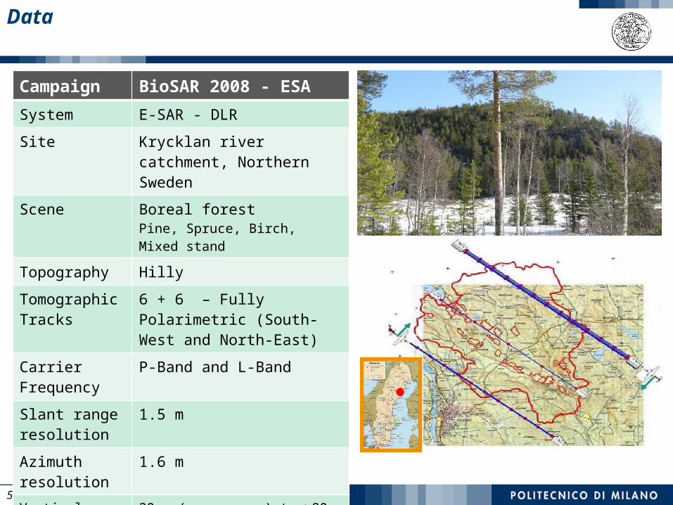
Campaign BioSAR 2008 - ESA
System E-SAR - DLR
Site Krycklan river catchment, Northern Sweden
Scene Boreal forestPine, Spruce, Birch, Mixed stand
Topography Hilly
Tomographic Tracks
6 + 6 – Fully Polarimetric (South-West and North-East)
Carrier Frequency
P-Band and L-Band
Slant range resolution
1.5 m
Azimuth resolution
1.6 m
Vertical resolution (P-Band)
20 m (near range) to >80 m (far range)
Vertical resolution (L-Band)
6 m (near range) to 25 m (far range)
5th Advanced Training Course in Land Remote Sensing
slant range, r
cross range,
v
Track 1
Track n
Track N
ground range
heig
ht
azimuth
Baseline
aperture
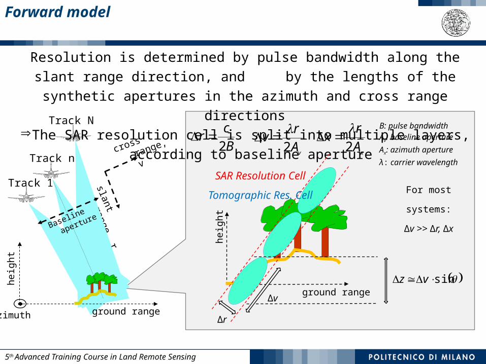
Resolution is determined by pulse bandwidth along the slant range direction, and
by the lengths of the synthetic apertures in the azimuth and cross range directionsÞ The SAR resolution cell is split into multiple layers, according to baseline aperture
B: pulse bandwidthAv: baseline aperture
Ax: azimuth aperture
λ: carrier wavelength
heig
ht
ground range
Δr
Δv
sin vz
For most systems:
Δv >> Δr, Δx
SAR Resolution Cell
Tomographic Res. Cell
B
cr
2
vA
rv
2
x
A
rx
2
Forward model
5th Advanced Training Course in Land Remote Sensing
yn(r,x) : SLC pixel in the n-th image
s(r,x,v): average complex reflectivity of the scene
within the SAR 2D resolution cell at (r,x)
bn : normal baseline for the n-th image
λ : carrier wavelength
dvvbr
jvxrsxrynn
4
exp,,,
Each focused SLC SAR image is obtained as the Fourier Transform of the scene
complex reflectivity along the cross-range coordinate
Vertical wavenumber
dzznjkzxrsxry zn exp,,,
sin
4 nz
b
rnk
Change of variable from cross range to height
kz is usually referred to as vertical wavenumber
or phase to height conversion factor
sinvz
cros
s ra
nge,
v
transmitted
pulse
Δr
Radar Line
of Sight
heig
ht, z
5th Advanced Training Course in Land Remote Sensing
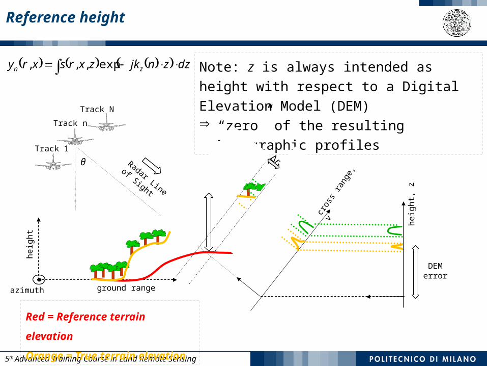
Reference height
dzznjkzxrsxry zn exp,,, Note: z is always intended as height with respect to
a Digital Elevation Model (DEM)Þ “zero” of the resulting Tomographic profiles
Track 1
Track n
Track N
ground range
heig
ht
azimuth
θ
cros
s ra
nge,
v
ΔrRadar Line
of Sight
heig
ht,
z
DEM error
Red = Reference terrain elevation
Orange = True terrain elevation
5th Advanced Training Course in Land Remote Sensing
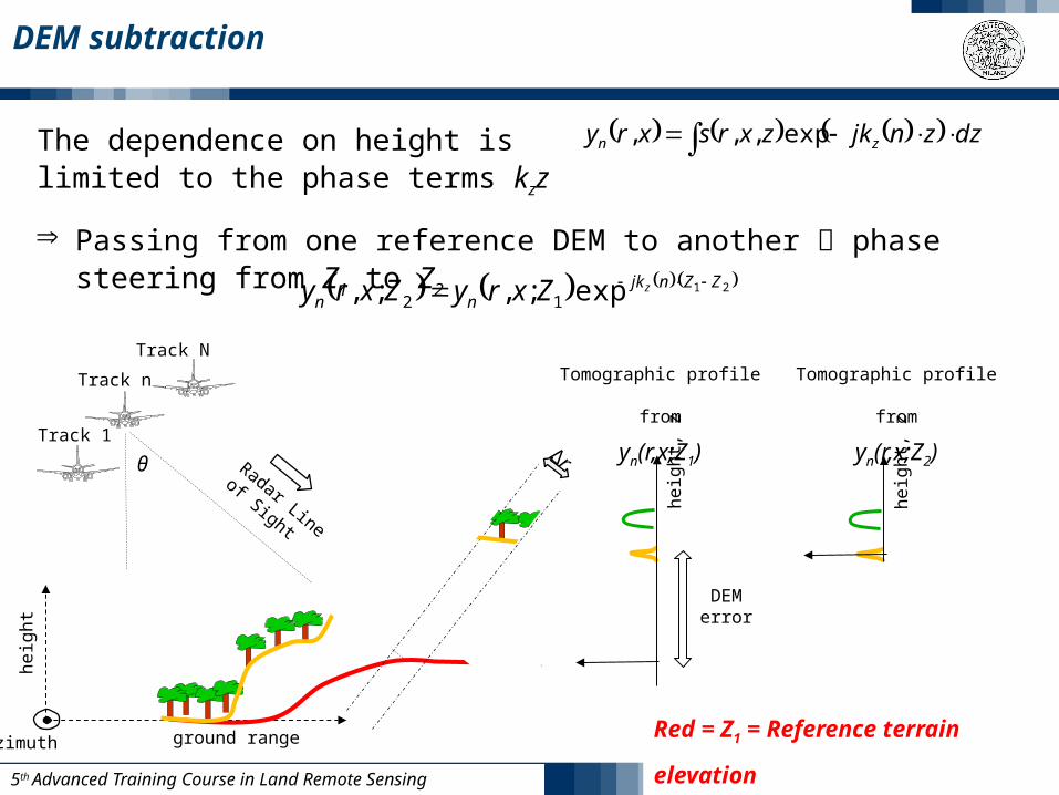
DEM subtraction
dzznjkzxrsxry zn exp,,,The dependence on height is limited to the phase terms kzz
Þ Passing from one reference DEM to another phase steering from Z1 to Z2
21exp;,;, 12ZZnjk
nnzZxryZxry
Red = Z1 = Reference terrain elevation
Orange = Z2 = True terrain elevation
Track 1
Track n
Track N
ground range
heig
ht
azimuth
θΔrRadar Line
of Sight
DEM error
heig
ht,
z
heig
ht,
z
Tomographic profile from
yn(r,x;Z1)
Tomographic profile from
yn(r,x;Z2)
5th Advanced Training Course in Land Remote Sensing
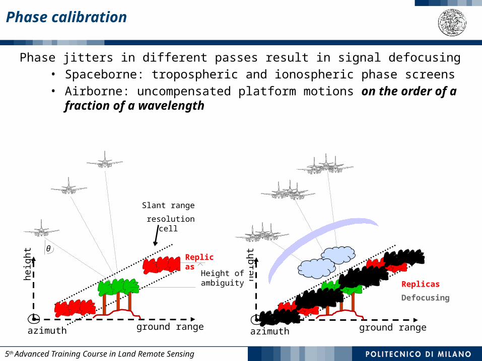
Phase calibration
ground range
heig
ht
azimuth
Slant range
resolution cell
ground range
heig
ht
azimuth
Replicas
Replicas
Defocusing
θ
Phase jitters in different passes result in signal defocusing• Spaceborne: tropospheric and ionospheric phase screens • Airborne: uncompensated platform motions on the order of a fraction of a
wavelength
Height of ambiguity
5th Advanced Training Course in Land Remote Sensing
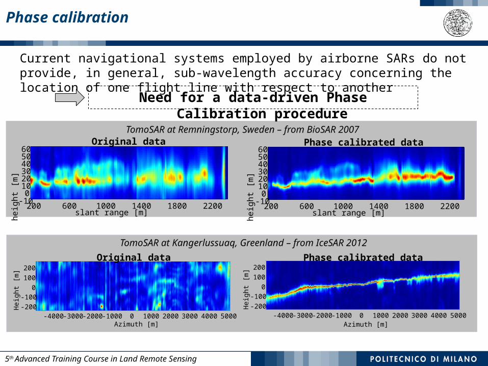
TomoSAR at Kangerlussuaq, Greenland – from IceSAR 2012
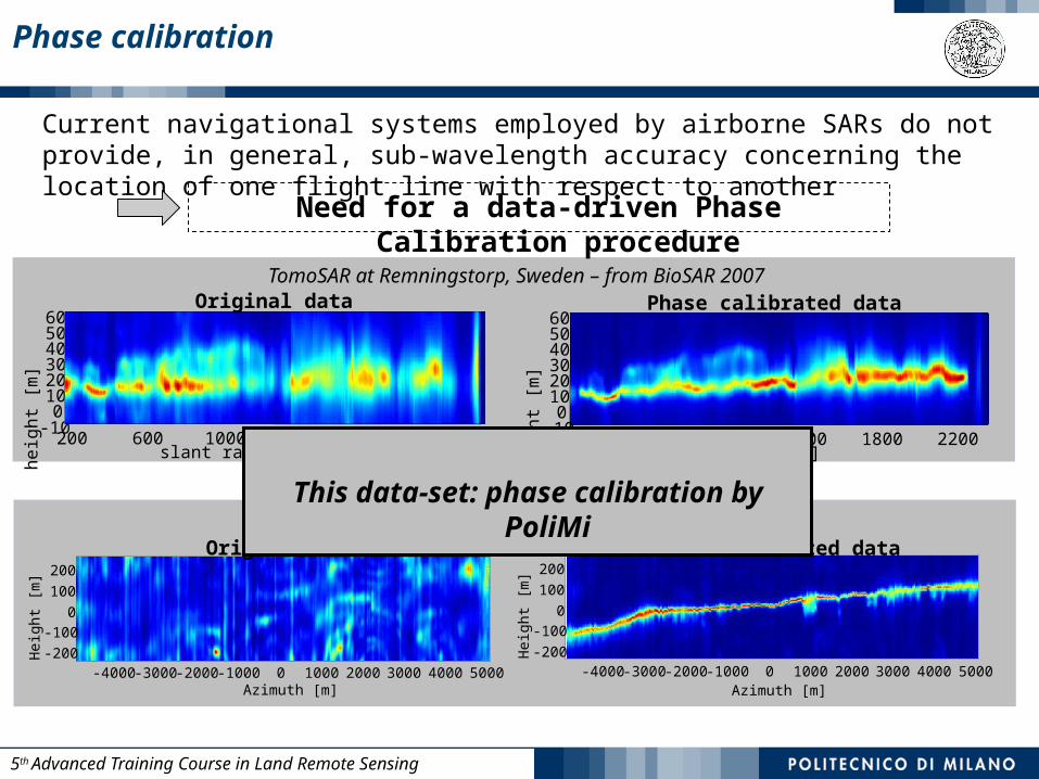
TomoSAR at Remningstorp, Sweden – from BioSAR 2007
slant range [m]he
igh
t [m
]
200 600 1000 1400 1800 2200-10
0102030405060
slant range [m]he
igh
t [m
]
200 600 1000 1400 1800 2200-10
0102030405060
Original data Phase calibrated data
Current navigational systems employed by airborne SARs do not provide, in general, sub-wavelength accuracy concerning the location of one flight line with respect to another
Need for a data-driven Phase Calibration procedure
5th Advanced Training Course in Land Remote Sensing
TomoSAR at Kangerlussuaq, Greenland – from IceSAR 2012
TomoSAR at Remningstorp, Sweden – from BioSAR 2007
slant range [m]he
igh
t [m
]
200 600 1000 1400 1800 2200-10
0102030405060
slant range [m]he
igh
t [m
]
200 600 1000 1400 1800 2200-10
0102030405060
Original data Phase calibrated data
Current navigational systems employed by airborne SARs do not provide, in general, sub-wavelength accuracy concerning the location of one flight line with respect to another
Need for a data-driven Phase Calibration procedure
This data-set: phase calibration by PoliMi
5th Advanced Training Course in Land Remote Sensing
TomoSAR_Main.m
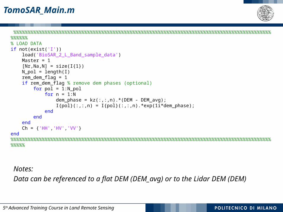
%%%%%%%%%%%%%%%%%%%%%%%%%%%%%%%%%%%%%%%%%%%%%%%%%%%%%%%%%%%%%%%%%%%%%%%%%%%%%%%%%%%%%%%%%%%%%%%%%% LOAD DATAif not(exist('I')) load('BioSAR_2_L_Band_sample_data') Master = 1 [Nr,Na,N] = size(I{1}) N_pol = length(I) rem_dem_flag = 1 if rem_dem_flag % remove dem phases (optional) for pol = 1:N_pol for n = 1:N dem_phase = kz(:,:,n).*(DEM - DEM_avg); I{pol}(:,:,n) = I{pol}(:,:,n).*exp(1i*dem_phase); end end end Ch = {'HH','HV','VV'}end%%%%%%%%%%%%%%%%%%%%%%%%%%%%%%%%%%%%%%%%%%%%%%%%%%%%%%%%%%%%%%%%%%%%%%%%%%%%%%%%%%%%%%%%%%%%%%%%%
Notes:
Data can be referenced to a flat DEM (DEM_avg) or to the Lidar DEM (DEM)
5th Advanced Training Course in Land Remote Sensing
TomoSAR_Main.m
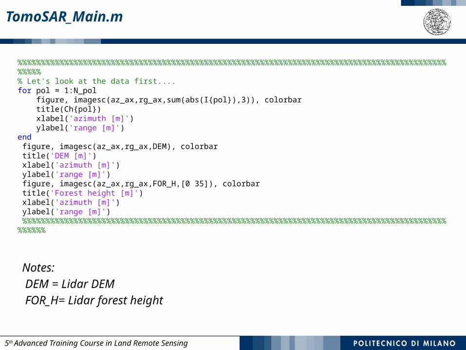
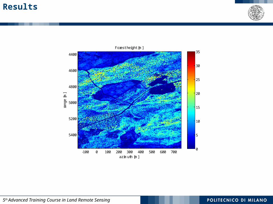
%%%%%%%%%%%%%%%%%%%%%%%%%%%%%%%%%%%%%%%%%%%%%%%%%%%%%%%%%%%%%%%%%%%%%%%%%%%%%%%%%%%%%%%%%%%%%%%%%% Let's look at the data first....for pol = 1:N_pol figure, imagesc(az_ax,rg_ax,sum(abs(I{pol}),3)), colorbar title(Ch{pol}) xlabel('azimuth [m]') ylabel('range [m]')end figure, imagesc(az_ax,rg_ax,DEM), colorbar title('DEM [m]') xlabel('azimuth [m]') ylabel('range [m]') figure, imagesc(az_ax,rg_ax,FOR_H,[0 35]), colorbar title('Forest height [m]') xlabel('azimuth [m]') ylabel('range [m]') %%%%%%%%%%%%%%%%%%%%%%%%%%%%%%%%%%%%%%%%%%%%%%%%%%%%%%%%%%%%%%%%%%%%%%%%%%%%%%%%%%%%%%%%%%%%%%%%%
Notes:
DEM = Lidar DEM FOR_H= Lidar forest height
5th Advanced Training Course in Land Remote Sensing
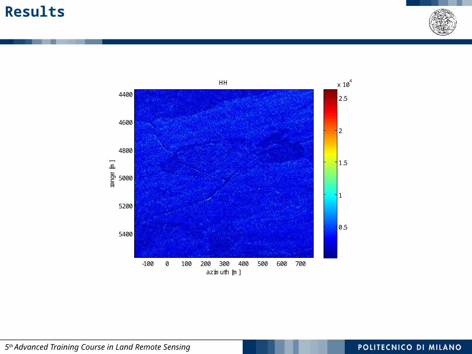
Results
azimuth [m]
rang
e [m
]
HH
-100 0 100 200 300 400 500 600 700
4400
4600
4800
5000
5200
54000.5
1
1.5
2
2.5
x 104
5th Advanced Training Course in Land Remote Sensing
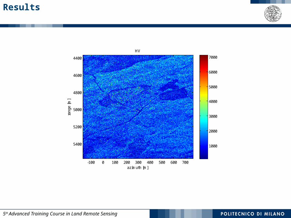
Results
azimuth [m]
rang
e [m
]
HV
-100 0 100 200 300 400 500 600 700
4400
4600
4800
5000
5200
5400 1000
2000
3000
4000
5000
6000
7000
5th Advanced Training Course in Land Remote Sensing
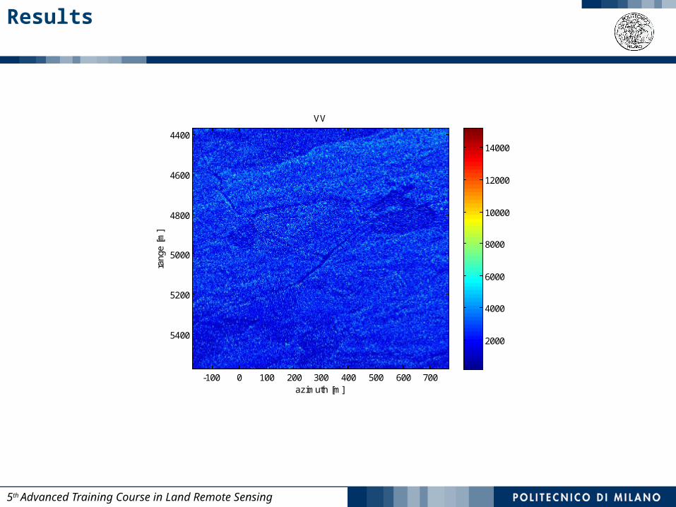
Results
azimuth [m]
rang
e [m
]
VV
-100 0 100 200 300 400 500 600 700
4400
4600
4800
5000
5200
54002000
4000
6000
8000
10000
12000
14000
5th Advanced Training Course in Land Remote Sensing
Results
azimuth [m]
rang
e [m
]
Forest height [m]
-100 0 100 200 300 400 500 600 700
4400
4600
4800
5000
5200
5400
0
5
10
15
20
25
30
35
5th Advanced Training Course in Land Remote Sensing
Results
azimuth [m]
rang
e [m
]
DEM [m]
-100 0 100 200 300 400 500 600 700
4400
4600
4800
5000
5200
5400
190
200
210
220
230
240
250
260
270
280
290
5th Advanced Training Course in Land Remote Sensing
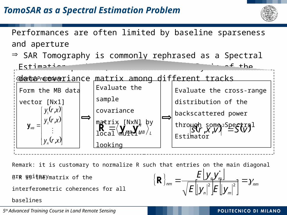
COV_4D is a 4D data structure representing the complex coherence as a function of each interferometric pair, i.e.: ynm(r,x)
Generate_covariance_matrix.m = function to evaluate COV_4D from SLC images
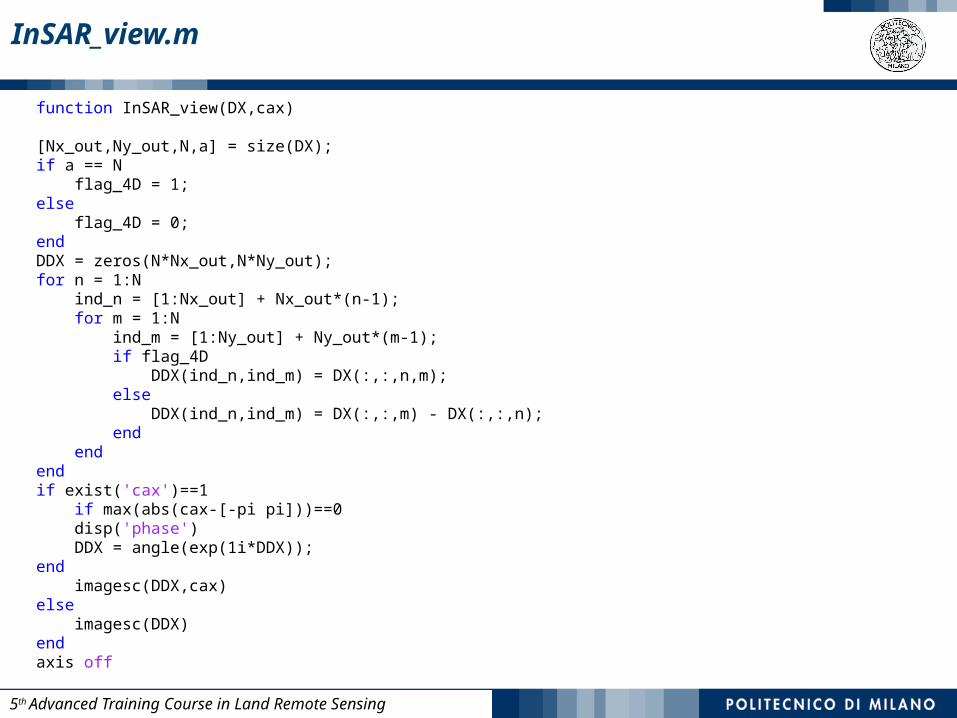
InSAR_view = function to view COV_4D as a big 2D matrix
5th Advanced Training Course in Land Remote Sensing
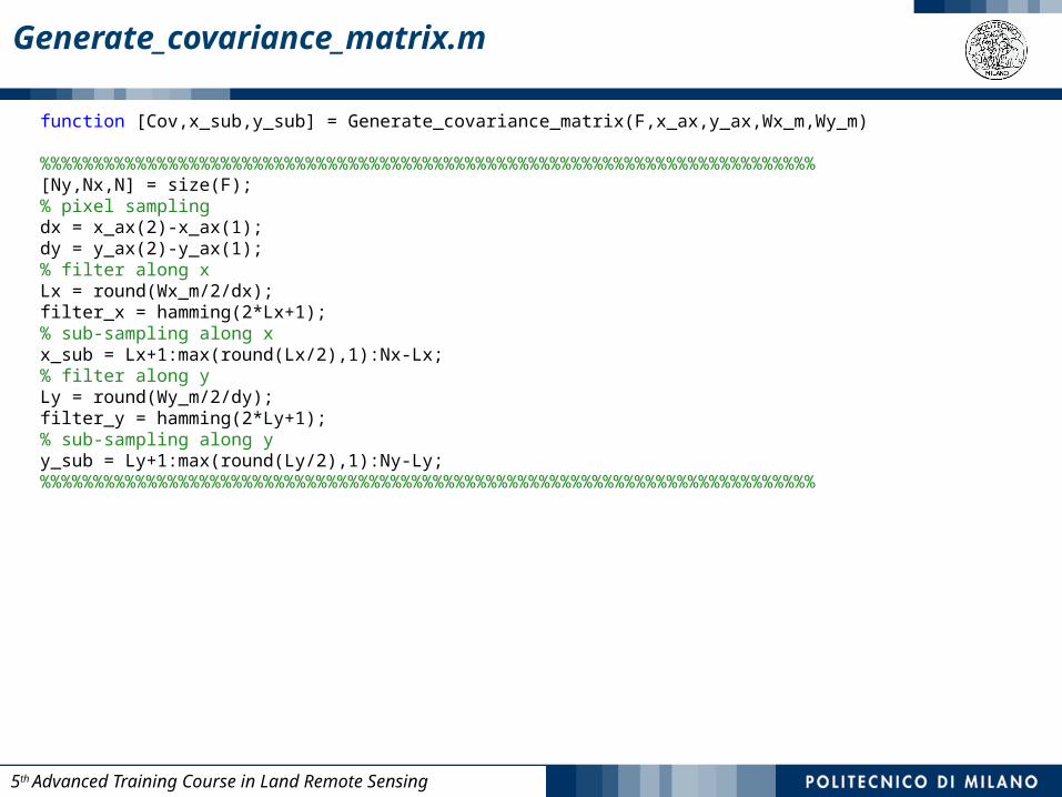
Generate_covariance_matrix.m
function [Cov,x_sub,y_sub] = Generate_covariance_matrix(F,x_ax,y_ax,Wx_m,Wy_m) %%%%%%%%%%%%%%%%%%%%%%%%%%%%%%%%%%%%%%%%%%%%%%%%%%%%%%%%%%%%%%%%%%%%%%%%%[Ny,Nx,N] = size(F);% pixel samplingdx = x_ax(2)-x_ax(1);dy = y_ax(2)-y_ax(1);% filter along xLx = round(Wx_m/2/dx);filter_x = hamming(2*Lx+1);% sub-sampling along xx_sub = Lx+1:max(round(Lx/2),1):Nx-Lx;% filter along yLy = round(Wy_m/2/dy);filter_y = hamming(2*Ly+1);% sub-sampling along yy_sub = Ly+1:max(round(Ly/2),1):Ny-Ly;%%%%%%%%%%%%%%%%%%%%%%%%%%%%%%%%%%%%%%%%%%%%%%%%%%%%%%%%%%%%%%%%%%%%%%%%%
5th Advanced Training Course in Land Remote Sensing
Generate_covariance_matrix.m
%%%%%%%%%%%%%%%%%%%%%%%%%%%%%%%%%%%%%%%%%%%%%%%%%%%%%%%%%%%%%%%%%%%%%%%%%% Covariance matrix evaluationNx_sub = length(x_sub);Ny_sub = length(y_sub);Cov = ones(Ny_sub,Nx_sub,N,N);for n = 1:N In = F(:,:,n); % n-th image % second-order moment Cnn = filter_and_sub_sample(In.*conj(In),filter_x,filter_y,x_sub,y_sub); for m = n:N Im = F(:,:,m); Cmm = filter_and_sub_sample(Im.*conj(Im),filter_x,filter_y,x_sub,y_sub); Cnm = filter_and_sub_sample(Im.*conj(In),filter_x,filter_y,x_sub,y_sub); % coherence coe = Cnm./sqrt(Cnn.*Cmm); Cov(:,:,n,m) = coe; Cov(:,:,m,n) = conj(coe); endend%%%%%%%%%%%%%%%%%%%%%%%%%%%%%%%%%%%%%%%%%%%%%%%%%%%%%%%%%%%%%%%%%%%%%%%%% %%%%%%%%%%%%%%%%%%%%%%%%%%%%%%%%%%%%%%%%%%%%%%%%%%%%%%%%%%%%%%%%%%%%%%%%%function Cnm = filter_and_sub_sample(Cnm,filter_x,filter_y,x_sub,y_sub)% filter and sub-samplet = Cnm;t = conv2(t,filter_x(:)','same');t = t(:,x_sub);t = conv2(t,filter_y(:),'same');t = t(y_sub,:);Cnm = t;%%%%%%%%%%%%%%%%%%%%%%%%%%%%%%%%%%%%%%%%%%%%%%%%%%%%%%%%%%%%%%%%%%%%%%%%%
5th Advanced Training Course in Land Remote Sensing
InSAR_view.m
function InSAR_view(DX,cax) [Nx_out,Ny_out,N,a] = size(DX);if a == N flag_4D = 1;else flag_4D = 0; endDDX = zeros(N*Nx_out,N*Ny_out);for n = 1:N ind_n = [1:Nx_out] + Nx_out*(n-1); for m = 1:N ind_m = [1:Ny_out] + Ny_out*(m-1); if flag_4D DDX(ind_n,ind_m) = DX(:,:,n,m); else DDX(ind_n,ind_m) = DX(:,:,m) - DX(:,:,n); end endendif exist('cax')==1 if max(abs(cax-[-pi pi]))==0 disp('phase') DDX = angle(exp(1i*DDX));end imagesc(DDX,cax)else imagesc(DDX)endaxis off
5th Advanced Training Course in Land Remote Sensing
Results – InSAR coeherences – DEM subtracted
InSAR coherences
0
0.1
0.2
0.3
0.4
0.5
0.6
0.7
0.8
0.9
1InSAR phases
-3
-2
-1
0
1
2
3
5th Advanced Training Course in Land Remote Sensing
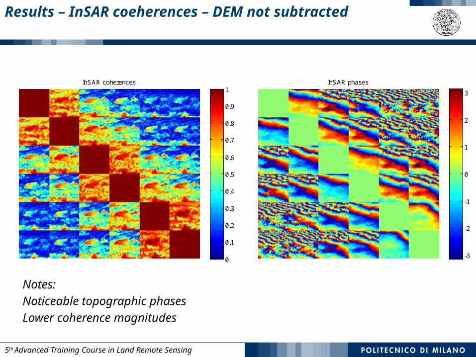
Results – InSAR coeherences – DEM not subtracted
InSAR coherences
0
0.1
0.2
0.3
0.4
0.5
0.6
0.7
0.8
0.9
1InSAR phases
-3
-2
-1
0
1
2
3
Notes:
Noticeable topographic phases
Lower coherence magnitudes
5th Advanced Training Course in Land Remote Sensing
TomoSAR_Main.m
%%%%%%%%%%%%%%%%%%%%%%%%%%%%%%%%%%%%%%%%%%%%%%%%%%%%%%%%%%%%%%%%%%%%%%%%%%%%%%%%%%%%%%%%%%%%%%%%%% TOMOGRAPHIC PROCESSING (3D focusing)% vertical axis (in meters)if rem_dem_flag % height w.r.t. DEM dz = 0.5; z_ax = [-20:dz:40];else % % height w.r.t. average DEM dz = 1; z_ax = [-150:dz:150];endNz = length(z_ax);% half the number of azimuth looks to be processedLx = 10% azimuth position to be processed (meters)az_profile_m = 590;az_profile_m = 678az_profile_m = -92% Focus in SAR geometryTomoSAR_focusingif rem_dem_flag == 0 % the following routines have been written assuming DEM phases are removed return end% Geocode to ground geometry and compare to Lidar forest heightGeocode_TomoSAR%%%%%%%%%%%%%%%%%%%%%%%%%%%%%%%%%%%%%%%%%%%%%%%%%%%%%%%%%%%%%%%%%%%%%%%%%%%%%%%%%%%%%%%%%%%%%%%%%
5th Advanced Training Course in Land Remote Sensing
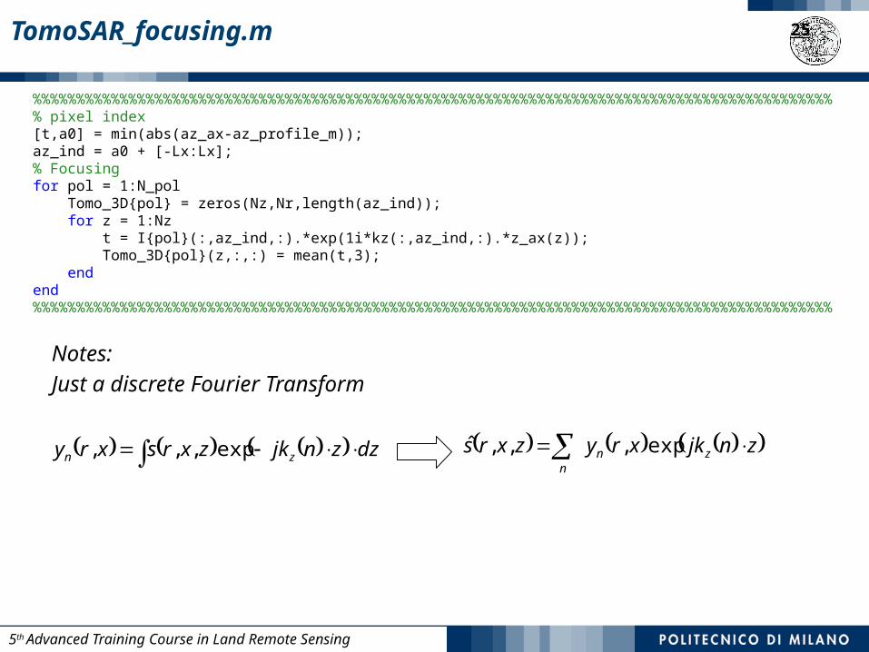
25TomoSAR_focusing.m
%%%%%%%%%%%%%%%%%%%%%%%%%%%%%%%%%%%%%%%%%%%%%%%%%%%%%%%%%%%%%%%%%%%%%%%%%%%%%%%%%%%%%%%%%%%%% pixel index[t,a0] = min(abs(az_ax-az_profile_m));az_ind = a0 + [-Lx:Lx];% Focusingfor pol = 1:N_pol Tomo_3D{pol} = zeros(Nz,Nr,length(az_ind)); for z = 1:Nz t = I{pol}(:,az_ind,:).*exp(1i*kz(:,az_ind,:).*z_ax(z)); Tomo_3D{pol}(z,:,:) = mean(t,3); endend%%%%%%%%%%%%%%%%%%%%%%%%%%%%%%%%%%%%%%%%%%%%%%%%%%%%%%%%%%%%%%%%%%%%%%%%%%%%%%%%%%%%%%%%%%%%
dzznjkzxrsxry zn exp,,, znjkxryzxrs znn
exp,,,ˆ
Notes:
Just a discrete Fourier Transform
5th Advanced Training Course in Land Remote Sensing
range [m]
heig
ht
[m]
HH
4400 4600 4800 5000 5200 5400-20
0
20
40
range [m]
heig
ht
[m]
HV
4400 4600 4800 5000 5200 5400-20
0
20
40
range [m]
heig
ht
[m]
VV
4400 4600 4800 5000 5200 5400-20
0
20
40
range [m]
heig
ht
[m]
HH
4400 4600 4800 5000 5200 5400-20
0
20
40
range [m]
heig
ht
[m]
HV
4400 4600 4800 5000 5200 5400-20
0
20
40
range [m]
heig
ht
[m]
VV
4400 4600 4800 5000 5200 5400-20
0
20
40
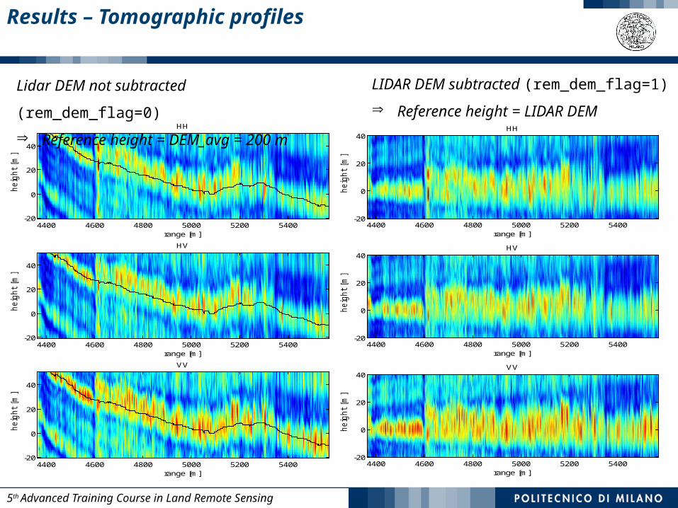
Results – Tomographic profiles
Lidar DEM not subtracted (rem_dem_flag=0)
Þ Reference height = DEM_avg = 200 m
LIDAR DEM subtracted (rem_dem_flag=1)
Þ Reference height = LIDAR DEM
5th Advanced Training Course in Land Remote Sensing
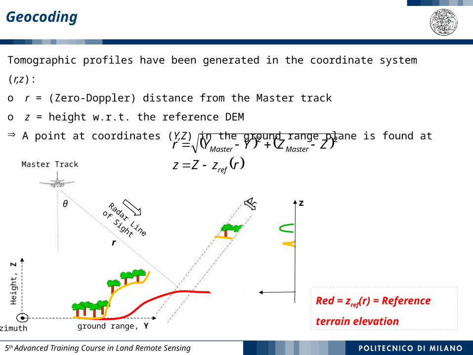
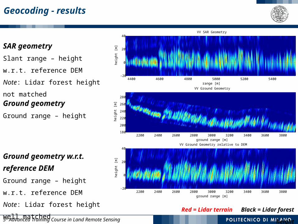
Geocoding
Red = zref(r) = Reference
terrain elevation
Master Track
ground range, Y
Heig
ht,
Z
azimuth
θΔrRadar Line
of Sight
z
r
Tomographic profiles have been generated in the coordinate system (r,z):
o r = (Zero-Doppler) distance from the Master track
o z = height w.r.t. the reference DEM
Þ A point at coordinates (Y,Z) in the ground range plane is found at
rzZz
ZZYYr
ref
MasterMaster
22
5th Advanced Training Course in Land Remote Sensing
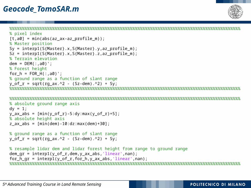
Geocode_TomoSAR.m
%%%%%%%%%%%%%%%%%%%%%%%%%%%%%%%%%%%%%%%%%%%%%%%%%%%%%%%%%%%%%%%%%%%%%%%%%%%%%%%%%%%%%%%%%%%%% pixel index[t,a0] = min(abs(az_ax-az_profile_m));% Master positionSy = interp1(S{Master}.x,S{Master}.y,az_profile_m);Sz = interp1(S{Master}.x,S{Master}.z,az_profile_m);% Terrain elevationdem = DEM(:,a0)';% Forest heightfor_h = FOR_H(:,a0)';% ground range as a function of slant rangey_of_r = sqrt(rg_ax.^2 - (Sz-dem).^2) + Sy;%%%%%%%%%%%%%%%%%%%%%%%%%%%%%%%%%%%%%%%%%%%%%%%%%%%%%%%%%%%%%%%%%%%%%%%%%%%%%%%%%%%%%%%%%%%%
%%%%%%%%%%%%%%%%%%%%%%%%%%%%%%%%%%%%%%%%%%%%%%%%%%%%%%%%%%%%%%%%%%%%%%%%%%%%%%%%%%%%%%%%%%%%% absolute ground range axisdy = 1;y_ax_abs = [min(y_of_r)-5:dy:max(y_of_r)+5];% absolute height axisz_ax_abs = [min(dem)-10:dz:max(dem)+30]; % ground range as a function of slant rangey_of_r = sqrt(rg_ax.^2 - (Sz-dem).^2) + Sy; % resample lidar dem and lidar forest height from range to ground rangedem_gr = interp1(y_of_r,dem,y_ax_abs,'linear',nan);for_h_gr = interp1(y_of_r,for_h,y_ax_abs,'linear',nan);%%%%%%%%%%%%%%%%%%%%%%%%%%%%%%%%%%%%%%%%%%%%%%%%%%%%%%%%%%%%%%%%%%%%%%%%%%%%%%%%%%%%%%%%%%%%
5th Advanced Training Course in Land Remote Sensing