1/68

System identification

Goal

A statistical framework

Noisy data

Model

Cost

2/68

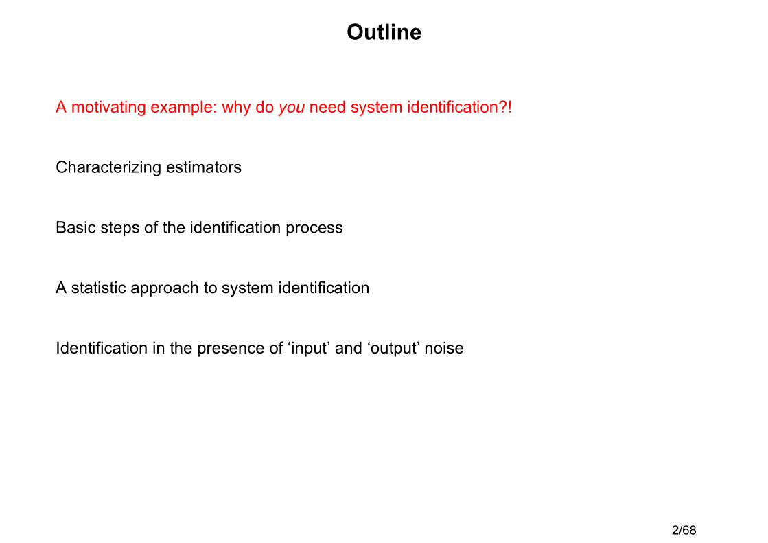
Outline

A motivating example: why do you need system identification?!

Characterizing estimators

Basic steps of the identification process

A statistic approach to system identification

Identification in the presence of ‘input’ and ‘output’ noise

3/68

Why do you need identification methods?

A simple experiment

4/68

Why do you need identification methods?

A simple experiment

Multiple measurements lead to conflicting results.

How to combine all this information?

5/68

Why do you need identification methodsMeasurement of a resistance

2 sets of measurements

u k( )

i k( )

6/68

3 different estimators

RSA N( ) 1N----

u k( )i k( )---------

k 1=Nå=

RLS N( )

1N----

u k( )i k( )k 1=Nå

1N----

i k( )2k 1=Nå

-----------------------------------------=

REV N( )

1N----

u k( )k 1=Nå

1N----

i k( )k 1=Nå

--------------------------------=

7/68

and their results

Remarks- variations decrease as function of , except for

- the asymptotic values are different

- behaves ‘strange’

N RSA

RSA

8/68

Repeating the experiments.

- the distributions become more concentrated around their limit value- behaves ‘strange’ for group A

Observed pdf of for both groups, from the left tot the rightR N( ) N 10 100 and 1000, ,=

RSA

9/68

Repeating the experiments.

- the standard deviation decrease in

- the uncertainty also depends on the estimator

GroupA

Standard deviation of

full dotted line: , dotted line: , full line: , dashedline .

R N( )

RSA RLS REV1 N¤

Group B

N

10/68

Strange behaviour of for group A.

- The current takes negative values for group A

- the estimators tend to a normal distributioneven when the noise behaviour is completely different

RSA

Group A Group B

Histogram of the current measurements.

11/68

Simplified analysis

Why do the asymptotic values depend on the estimator?

Can we explain the behaviour of the variance?

Why does the estimator behave strange for group A?

More information is needed to answer these questions

RSA

12/68

Noise model of the measurements

Assumptions:

and are:

- mutually independent- zero mean- independent and identically distributed- have a symmetric distribution- variance and .

i k( ) i0 ni k( )+= u k( ) u0 nu k( )+=

ni k( ) nu k( )

su2 si

2

13/68

Statistical tools

1N----

x k( )k 1=NåN ¥®

lim 0=

1N----

x k( )2k 1=NåN ¥®

lim sx2=

1N----

x k( )y k( )k 1=NåN ¥®

lim 0=

14/68

Asymptotic value of

Or

And finally

It converges to the wrong value!!!

RLS

RLS N( )N ¥®lim u k( )i k( )

k 1=Nåè ø

æ ö i2 k( )k 1=Nåè ø

æ ö¤N ¥®lim=

1N----

u0 nu k( )+( ) i0 ni k( )+( )k 1=Nå1N----

i0 ni k( )+( )2k 1=Nå

-------------------------------------------------------------------------------N ¥®lim=

RLS N( )N ¥®lim =

u0i0u0N-----

ni k( )k 1=Nå

i0N----

nu k( )k 1=Nå 1

N----nu k( )ni k( )

k 1=Nå+ + +

i02 1

N----ni

2 k( )k 1=Nå

2i0N-------

ni k( )k 1=Nå+ +

----------------------------------------------------------------------------------------------------------------------------------------------------N ¥®lim

RLS N( )N ¥®lim

u0i0i02 si

2+----------------- R0

1

1 si2 i0

2¤+------------------------= =

15/68

Asymptotic value of

It converges to the exact value!!!

REV

REV N( )N ¥®lim u k( )

k 1=Nåè ø

æ ö i k( )k 1=Nåè ø

æ ö¤N ¥®lim=

1N----

u0 nu k( )+( )k 1=Nå

1N----

i0 ni k( )+( )k 1=Nå

----------------------------------------------------N ¥®lim=

u01N----

nu k( )k 1=Nå+

i01N----

ni k( )k 1=Nå+

-----------------------------------------------N ¥®lim

è øç ÷ç ÷ç ÷æ ö

=

R0=

16/68

Asymptotic value of

The series expansion exist only for small noise distortions

for

Group A: The expected value does not exist for the data of group A.The estimator does not converge.

Group B: For group B the series converges and

The estimator converges to the wrong value!!

RLS

RSA N( ) 1N----

u k( )i k( )---------

k 0=Nå 1

N----u0 nu k( )+i0 ni k( )+------------------------

k 0=Nå 1

N----u0i0-----

1 nu k( ) u0¤+1 ni k( ) i0¤+-------------------------------

k 0=Nå= = =

11 x+------------ 1–( )lxl

l 0=¥å= x 1<

RSA N( )N ¥®lim R0 1

si2

i02------+

è øç ÷ç ÷æ ö

»

17/68

Variance expressions

First order approximation

- variance decreases in

- variance increases with the noise

- for low noise levels, all estimators have the same uncertainty

---> Experiment design

sRLS

2 N( ) sREV

2 N( ) sRSA

2 N( )R0

2

N------su

2

u02------

si2

i02------+

è øç ÷ç ÷æ ö

» » »

1 N¤

18/68

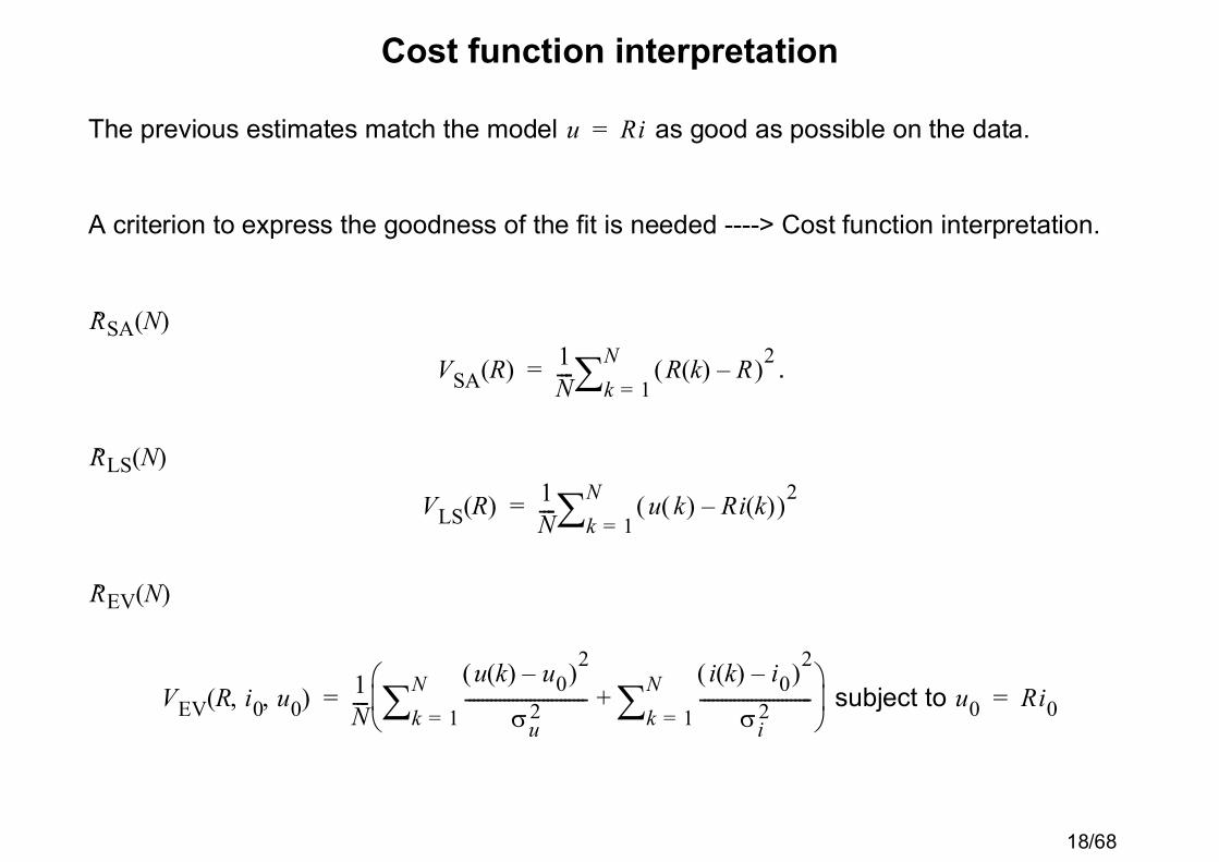
Cost function interpretation

The previous estimates match the model as good as possible on the data.

A criterion to express the goodness of the fit is needed ----> Cost function interpretation.

.

subject to

u Ri=

RSA N( )

VSA R( ) 1N----

R k( ) R–( )2k 1=Nå=

RLS N( )

VLS R( ) 1N----

u k( ) Ri k( )–( )2k 1=Nå=

REV N( )

VEV R i0 u0, ,( ) 1N----

u k( ) u0–( )2

su2----------------------------

k 1=Nå

i k( ) i0–( )2

si2--------------------------

k 1=Nå+

è øç ÷æ ö

= u0 Ri0=

19/68

Conclusion

- A simple problem

- Many solutions

- How to select a good estimator?

- Can we know the properties in advance?

Need for a general framework !!

20/68

Outline

A motivating example: why do you need system identification?!

Characterizing estimators

Basic steps of the identification process

A statistic approach to system identification

Identification in the presence of ‘input’ and ‘output’ noise

21/68

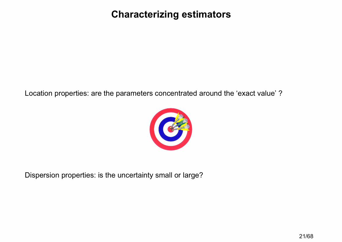
Characterizing estimators

Location properties: are the parameters concentrated around the ‘exact value’ ?

Dispersion properties: is the uncertainty small or large?

22/68

Location properties

unbiased and consistent estimators

Unbiased estimates

the mean value equals the exact value

DefinitionAn estimator of the parameters is unbiased if , for alltrue parameters . Otherwise it is a biased estimator.

Asymptotic unbiased estimates: unbiased for

q q0 E q{ } q0=q0

N ¥®

23/68

Example

i) The sample mean

Unbiased?

ii) The sample variance

Unbiased?

Alternative expression

u N( ) 1N----

u k( )k 1=Nå=

E u N( ){ } 1N----

E u k( ){ }k 1=Nå 1

N----u0k 1=

Nå u0= = =

su2 N( ) 1

N----u k( ) u N( )–( )2

k 1=Nå=

E {su2 N( )} N 1–

N-------------su2=

1N 1–------------- u k( ) u N( )–( )2

k 1=Nå

24/68

Example cont’d

and

bias , and bias

variance > variance

RMS error > RMS error

Best choice?

s12 1

N 1–------------- u k( ) u N( )–( )2k 1=Nå= s2

2 1N----

u k( ) u N( )–( )2k 1=Nå=

s12 0= s2

2 s2

N------=

s12 s2

2

s12 s2

2

25/68

Consistent estimates

Consistent estimates: the probability mass gets concentrated around the exact value

or

ProbN ¥®lim q N( ) q0– d 0> >( ) 0=

q N( )N ¥®plim q0=

Consistency

properties

if all plim exist

plim f a( ) f plim a( )=

plim ab plim a plim b=

27/68

Example

REV N( )N ¥®plim

1N----

u k( )k 1=Nå

1N----

i k( )k 1=Nå

--------------------------------N ¥®plim=

1N----

u k( )k 1=Nåè ø

æ öN ¥®plim

1N----

i k( )k 1=Nåè ø

æ öN ¥®plim-------------------------------------------------=

u0i0-----=

R0=

28/68

Dispersion properties

efficient estimators

- Mostly the covariance matrix is used, however alternatives like percentiles exist.

- For a given data set, there exists a minimum bound on the covariance matrix:

the Cramér-Rao lower bound.

with

.

The derivatives are calculated in

CR q( ) Fi 1– q0( )=

Fi q0( ) E q¶¶ l Z q( )è ø

æ öT

q¶¶ l Z q( )è ø

æ öî þí ýì ü

Eq2

2

¶

¶ l Z q( )–î þí ýì ü

–= =

q q0=

29/68

The likelihood function

1) Consider the measurements

2) is generated by a hypothetical, exact model with parameters

3) is disturbed by noise --> stochastic variables

4) Consider the probability density function with

.

5)Interpret this relation conversely, viz:

how likely is it that a specific set of measurements aregenerated by a system with parameters ?

--> Measurements givenModel parameters as the free variables:

, with the free variables

: likelihood function.

Z RNÎ

Z q0

Z

f Z q0( )

f Z q0( ) Zdz RNÎò 1=

Z Zm=q

L Zm q( ) f Z Zm= q( )= q

L Zm q( )

30/68

Interpretation of the Cramér-Rao lower boundModel

Measurement and

Likelihood function

Loglikelihood function

Information matrix

y0 f u0 q,( )=

y y0 ny+= ny N 0 s2,( )~

L y q( ) fn y q( ) 1

2ps2-----------------e

y f u0 q,( )–( )2

2s2--------------------------------–= =

l y q( ) 12---

2ps2( )log–y f u0 q,( )–( )2

2s2---------------------------------–=

q¶¶l y f u0 q,( )–( )

s2------------------------------- q¶¶ f u0 q,( )–=

Fi q0( ) Eq¶

¶lè øæ öT

q¶¶lè øæ ö

î þí ýì ü

=

Ey f u0 q,( )–( )2

s4--------------------------------- q¶¶ f u0 q,( )è ø

æ ö 2

î þí ýì ü

=

1s2------ q¶

¶ f u0 q,( )è øæ ö 2

=

31/68

32/68

33/68

34/68

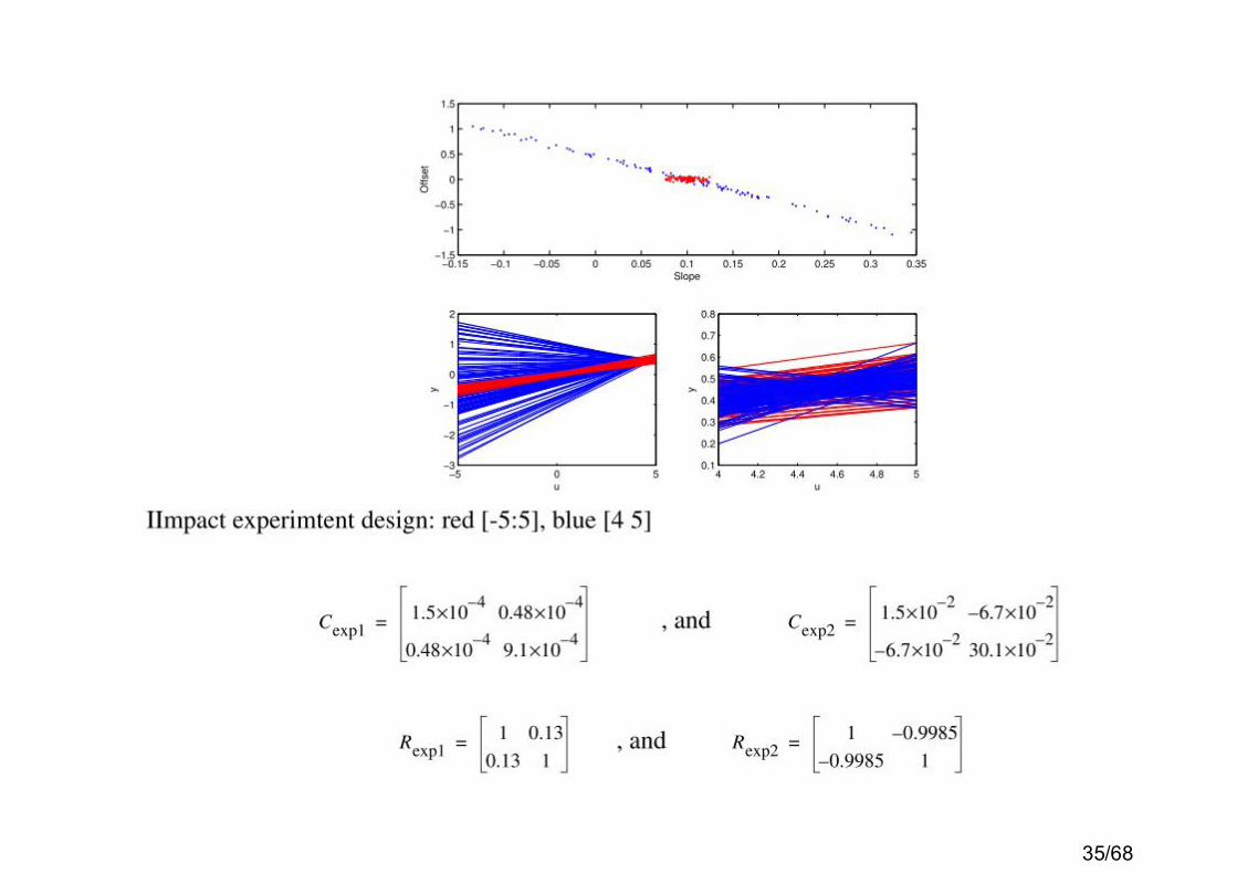
35/68

36/68

37/68

Characterizing estimators

• Goal asymptotic analysis- what happens with the estimate if more data are gathered?- hypothesis: asymptotic behaviour reflects finite sample behaviour- true finite sample behaviour is in general very difficult to establish

(exception: linear least squares)

• Consistency- convergence in stochastic sense to the true value- does not exclude divergence for some realisations- guarantees with high probability that estimate is close to true value- consistency does not imply asymptotic unbiasedness- proof: law of large numbers

• Asymptotic unbiasedness- asymptotically the expected value equals the true value- does not guarantee that the estimate is close to the true value- in general very difficult to verify (exception: linear least squares)

• Asymptotic normality- allows to construct uncertainty bounds with a given confidence level- proof: linearisation around limit value + central limit theorem

38/68

Characterizing estimators (Cont’d)

• Asymptotic variance- measure of the convergence rate- construction of uncertainty bounds- proof: linearisation around limit value

• Asymptotic efficiency- minimal uncertainty within class of asymptotically unbiased estimators- in practice applied to class of consistent estimators- Cramér-Rao lower bound does not always exist

or may be too conservative- proof: comparison asymptotic variance with Cramér-Rao lower bound

• Robustness- sensitivity (asymptotic) properties to the noise assumptions- proof: validity law of large numbers and central limit theorem

under relaxed noise assumptions

39/68

Outline

A motivating example: why do you need system identification?!

Characterizing estimators

Basic steps of the identification process

A statistic approach to system identification

Identification in the presence of ‘input’ and ‘output’ noise

40/68

Basic steps in identification

1) collect the information: experiment setup

2) select a modelparametric >< nonparametric modelswhite>< black box modelslinear><nonlinear modelslinear -in-the-parameters><nonlinear-in-the-parameters

,

3) match the model to the data

select a cost functionLS, WLS, MLE, Bayes estimation

4) validationdoes the model explain the data?can it deal with new data?

Remarkthis scheme is not only valid for the classical identification theory.It also applies to neural nets, fuzzy logic, ...

e y a1u a2u2+( )–= e w( ) Y w( )a0 a1jw+b0 b1jw+------------------------U w( )–=

41/68

Outline

A motivating example: why do you need system identification?!

Characterizing estimators

Basic steps of the identification process

A statistic approach to system identification

Identification in the presence of ‘input’ and ‘output’ noise

42/68

A statistical framework: choice of the cost functions

, ,

Least squares estimation

Weighted least squares estimation

Maximum likelihood estimation

y0 G u q0,( )= y y0 ny+= e y G u q0,( )–=

VLS q( ) 1N----

e2 k q,( )k 1=Nå=

VWLS q( ) 1N----

e q( )TWe q( )=

f y q0( ) fnyy G u q0,( )–( )=

qML argmaxf ym q( )q

=

43/68

Least squares: principle

Model

with the measurement index, and

, ,

Measurements

Match model and measurementsChoose:

,with the modelled output.

Then,

with

y0 k( ) g u0 k( ) q,( )=

k

y k( ) RÎ u k( ) R1xMÎ q Rnqx1Î

y k( ) y0 k( ) ny k( )+=

e k q,( ) y k( ) y k q,( )–=y k q,( )

qLS VLS q( )q

arg min=

VLS q( ) 1N----

e2 k q,( )k 1=Nå=

44/68

Least squares: special casemodel that is linear-in-the-parameters

,

y0 K u0( )q0=

e q( ) y K u( )q–= K q¶¶e–=

qLS KTK( )1–KTy=

45/68

Properties

Noise assumptions with

Bias?

Note that

qLS KTK( )1–KTy=

y y0 ny+= E ny[ ] 0=

E qLS[ ] E KTK( )1–KTy=

KTK( )1–KTE y[ ]=

KTK( )1–KTy0=

y0 Kq0=

E qLS[ ] KTK( )1–KTKq0 q0= =

46/68

Properties

Noise assumptions with

Noise sensitivity?

Note

Covariance matrix

Asymptotical normal distributed

qLS KTK( )1–KTy=

y y0 ny+= E ny[ ] 0=

qLS q0– KTK( )1–KTny=

1N----

KT

Kè øæ ö 1– 1

N----K

Tny=

1N----

KT

nyN ¥®lim N 0 KTCy

N2------K,( )~

Cq1N----

KT

Kè øæ ö 1–

KTCy

N2------K 1N----

KT

Kè øæ ö 1–

=

47/68

Example: weight of a loaf of bread

model

measurements

estimator

Standard formulation

with

Solution

, for white noise

y0 q0=

y k( ) y0 ny k( )+=

e k( ) y k( ) q–=

y Kq ny+= K 1 1 ... 1, , ,( )T=

qLS KTK( )1–KTy 1

N----y k( )

k 1=Nå= =

sq2 1

N----K

TKè ø

æ ö 1–KTCy

N2------K 1N----

KT

Kè øæ ö 1– sy

2

N------= =

48/68

Example: weight of a loaf of bread (Cont’d)

measurements,

noise uniformly distributed

y k( ) y0 ny k( )+= k 1 ¼ N, ,=

50 50,–[ ]

1

2

4

8

49/68

Weighted least squares

Goal: bring your confidence in the measurements into the problem

Model

, ,

Measurements

confidence in measurement :

Match model and measurements,

Then,

with

y0 k( ) g u0 k( ) q,( )=

y k( ) RÎ u k( ) R1xMÎ q Rnqx1Î

y k( ) y0 k( ) ny k( )+=

k w k( )

e k q,( ) y k( ) y k q,( )–=

qLS VLS q( )q

arg min=

VWLS q( ) 1N----

e2 k q,( )w k( )------------------

k 1=Nå=

50/68

Weighted least squares (continued)

Generalization: use a full matrix to weight the measurements

define

consider a positive definite matrix

Then

Special choice:

This choice minimizes

e q( ) e 1 q,( )¼e N q,( )( )=

W

VWLS q( ) 1N----

e q( )TW 1– e q( )=

W nynyT}E { Cnyny

RNxNÎ= =

Cq

51/68

Example: resistor measurement, 2 voltmeters

,

uniformly distributed in

Voltmeter 1: , Voltmeter 2:

i k( ) i0 k( )=

u k( ) u0 k( ) nu k( )+=k 1 2 ¼ 100, , ,=

i0 0 0.01,[ ]

R0 1000=

N 0 su2=1,( ) N 0 su

2=32,( )

52/68

Maximum likelihood estimation

Model

, ,

Measurements

with the pdf of the noise

Match model and measurementsChoose the experiments such that the model becomes most likely:

Then

with

y0 k( ) g u0 k( ) q,( )=

y k( ) RÎ u k( ) R1xMÎ q Rnqx1Î

y k( ) y0 k( ) ny k( )+=

fnyny

qML f ym q u,( )q

arg max=

f y q u,( ) fnyy G u q,( )–( )=

53/68

Maximum likelihood: exampleweight of a loaf of bread

Model:

Measurements:

Additional informationThe distribution of is normal with zero mean and standarddeviation

Likelihood function:

Maximum likelihood estimator:

y0 q0=

y k( ) y0 ny k( )+=

fy nysy

f y q( ) 1

2psy2

-----------------e

y q–( )2

2sy2------------------–

1

2psy2N---------------------e

12sy

2--------- y k( ) q–( )2

k 1=Nå–

= =

qML1N----

y k( )k 1=Nå=

54/68

Resistance example with Gaussian and Laplace noisewhite Gaussian noise

--> least squares

white Laplace noise

--> least absolute values

u k( ) Ri k( )– 2k 1=NåR

arg min

u k( ) Ri k( )–k 1=NåR

arg min

Least Squares

Least Abs ValuesGaussian

Laplace

55/68

Properties of the Maximum likelihood estimator

principle of invariance: if is a MLE of , then is a MLE of

where is a function, and , with a finite number.

consistency: if is an MLE based on iid random variables, with independent

of , then converges to almost surely: .

asymptotic normality: if is a MLE based on iid random variables, with

independent of , then converges in law to a normal random variable with the

Cramér-Rao lower bound as covariance matrix.

qML q RnqÎ qg g qML( )= g q( )

g qg RngÎ ng nq£ nq

qML N( ) N nqN qML q0 qML N( )

N ¥®a.s.lim q0=

qML N( ) N nqN qML N( )

56/68

Bayes estimator: principle

Choose the parameters that have the highest probability:

Problem: prior distribution of the parameters is required

q arg f q u y,( )q

max=

f q u y,( )f y q u,( )f q( )

f y( )-----------------------------=

57/68

Bayes estimator: example 1

Use of Bayes estimators in our daily life

58/68

Bayes estimator: example 2weight of a loaf of bread

Model:

Measurements:

Additional information 1: disturbing noiseThe distribution of is

Additional information 2: prior distribution of the parametersThe bread is normally distributed:

Bayes estimator:

y0 q0=

y k( ) y0 ny k( )+=

fy ny N 0 sy2,( )

N 800gr sw,( )

f y q( )f q( ) 1

2psy2

-----------------e

y q–( )2

2sy2------------------–

1

2psw2

------------------e

q w–( )2

2sw2--------------------–

=

qz sy

2¤ w sw2¤+

1 sy2¤ 1 sw

2¤+----------------------------------=

59/68

Example continued

After making several independent measurements

the Bayes estimator becomes

For a large number of measurements:

y 1( ) ¼ y N( ), ,

f y q( )f q( ) 1

2psy2

è øæ ö

N--------------------------e

y k( ) q–( )2

2sy2-------------------------

k 1=

Nå– 1

2psw2

------------------e

q w–( )2

2sw2--------------------–

=

qy k( ) sy

2¤k 1=Nå w sw

2¤+

N sy2¤ 1 sw

2¤+-----------------------------------------------------------=

qy k( ) sy

2¤k 1=Nå

N sy2¤

-------------------------------------- 1N----

y k( )k 1=Nå= =

60/68

Outline

A motivating example: why do you need system identification?!

Characterizing estimators

Basic steps of the identification process

A statistic approach to system identification

Identification in the presence of ‘input’ and ‘output’ noise

61/68

Identification in the presence of input and output noise

Model

Measurements

Multiple solutions- MLE formulation --> errors-in-variables EIV- instrumental variables- total least squares

y0 k( ) g u0 k( ) q0,( )=

u k( ) u0 k( ) nu k( )+=

y k( ) y0 k( ) ny k( )+=

62/68

Problem

Noise on the regressor --> systematic errors

(0-1)

or in general

RLS N( )

1N----

u k( )i k( )k 1=Nå

1N----

i2 k( )k 1=Nå

-----------------------------------------=

RLS N( )N ¥®lim R0

11 si

2 i02¤+

------------------------=

qLS N( ) KTK( ) 1– KTy=

quadratic terms --> bias

63/68

Errors-in-variables(MLE)

Model

Measurements

, pdf of the noise

for simplicity:

Cost: likelihood function

with

Parametersthe model parametersthe unknown, true input and output:Note that the number of parameters depends on !!!!!

y0 k( ) g u0 k( ) q0,( )=

u k( ) u0 k( ) nu k( )+=

y k( ) y0 k( ) ny k( )+=

nu --> fnu

ny --> fny

f nu ny,( ) fnufnu

=

f y u,( )| y0 u0 q0, ,( )( ) fnyy y0– |y0 q0,( )fnu

u u0– |u0 q0,( )=

y0 k( ) g u0 k( ) q0,( )=

q0u0 k( ) y0 k( ),

N

64/68

EIV

Example: Resistance

model

measurements

noise model i.i.d. zero mean normally distributed

u0 k( ) Ri0 k( )=

u k( ) u0 k( ) nu k( )+=

i k( ) i0 k( ) ni k( )+=

nu k( ) ni k( ),

nu k( ) --> N 0 su2,( )

ni k( ) --> N 0 si2,( )

65/68

Example EIV (cont’d)likelihood function

with

or

The cost function becomes

with

f i u,( ) | i0 u0 q0, ,( )( ) fnii y0– |y0 q0,( )fnu

u u0– |u0 q0,( )=

u0 k( ) Ri0 k( )=

1

2psi2( )N

--------------------------e

i k( ) i0 k( )–( )2

si2-------------------------------

k 1=

N

å–1

2psu2( )N

--------------------------e

u k( ) u0 k( )–( )2

su2----------------------------------

k 1=

N

å–

VMLE i u q, ,( )i k( ) i0 k( )–( )2

si2---------------------------------

u k( ) u0 k( )–( )2

su2-----------------------------------+

k 1=Nå=

u0 k( ) Ri0 k( )=

66/68

Example EIV (cont’d)

Elimination of

Solution

,

compare to the Least Squares estimator

i0 u0,

VMLE i u q, ,( ) Ri k( ) u k( )–( )2

su2 Rsi

2+-----------------------------------

k 1=Nå=

REIV

u k( )2åsu

2-------------------i k( )2åsi

2------------------–u k( )2åsu

2-------------------i k( )2åsi

2------------------–è øç ÷æ ö 2

4u k( )i k( )å( )2

su2si

2---------------------------------++

u k( )i k( )åsu

2--------------------------------------------------------------------------------------------------------------------------------------------------------------------------------=

RLS

u k( )i k( )k 1=Nå

i k( )2k 1=Nå

------------------------------------=

67/68

Example: Resistance

, , ,R0 1000= i0: N 0 0.012,( ) si2 0.0012= su

2 1=

68/68

Outline

A motivating example: why do you need system identification?!

Characterizing estimators

Basic steps of the identification process

A statistic approach to system identification

Identification in the presence of ‘input’ and ‘output’ noise