1 System-Level Design Methodology Daniel D. Gajski Center for Embedded Computer Systems University of California, Irvine www.cecs.uci.edu/~gajski Abstract With complexities of Systems-on-Chip rising almost daily, the design community has been searching for new methodology that can handle given complexities with increased productivity and decreased times-to-market. The obvious solution that comes to mind is increasing levels of abstraction, or in other words, increasing the size of the basic building blocks. However, it is not clear what these basic blocks should be beyond the obvious processors and memories. Furthermore, with multitude of processors and variety of IPs on the chip the difference between SW and HW design becomes indistinguishable. However, the industry infrastructure which is also supported by separate SW and HW programs being offered at our universities created the system gap in which non-compatible SW and HW methodologies are preventing the progress in design of electronic systems. In this talk we will present the basic principles of system methodologies and describe the methodology based on SER paradigm. In order to prove the SER concept we developed the SCE system design environment and demonstrated in practice more then 1000X productivity gain.
Transcript
1
System-Level Design Methodology
Daniel D. GajskiCenter for Embedded Computer Systems
University of California, Irvinewww.cecs.uci.edu/~gajski
Abstract
With complexities of Systems -on-Chip rising almost daily, the design community has been searching for new methodology that can handle given complexities with increased productivity and decreased times-to-market. The obvious solution that comes to mind is increasing levels of abstraction, or in other words, increasing the size of the basic building blocks. However, it is not clear what these basic blocks should be beyond the obvious processors and memories. Furthermore, with multitude of processors and variety of IPs on the chip the difference between SW and HW design becomes indistinguishable. However, the industry infrastructure which is also supported by separate SW and HW programs being offered at our universities created the system gap in which non-compatible SW and HW methodologies are preventing the progress in design of electronic systems. In this talk we will present the basic principles of system methodologies and describe the methodology based on SER paradigm. In order to prove the SER concept we developed the SCE system design environment and demonstrated in practice more then 1000X productivity gain.
2
Copyright 2003 Daniel D. Gajski 2
Outline
• System gap• Design flow• Model algebra• System environment• Vision• Conclusion
Outline
In order to find the solution for system-level design flow, we will look first at the system gap between SW and HW designs and then try to bridge this gap by looking at different levels of abstraction, define different models on each level and propose model refinements that will bring the specification to a cycle-accurate implementation. In order to achieve this design flow we will define the models in the flow by using the concepts of model algebra similar to concepts of arithmetic algebras that are defined on a set of numbers. Then, we will exemplify these concepts by looking into the implementation of the System-on-Chip Environment and the lessons learned from several experiments. We will finish with a prediction and a roadmap to achieve the ultimate goal of increasing system-design productivity by more then 1000X and reducing expertise level needed for such design to the basic principles of design science only.
3
Copyright 2003 Daniel D. Gajski 3
Past, Present and Future Design Flow
Simulate
Physical
Logic
Specs
Design
Manufacturing
Algorithms
System Gap
1960’s
SW?
Capture& Simulate
Communications
Functionality
Connectivity
Protocols
Timing
Architecture
Manufacturing
Executable Spec
Algorithms
Physical
Logic
SW/HW Design
2000’s
Network
Algorithms
Performance
Specify, Explore& Refine
Describe
Simulate
Manufacturing
Specs
Algorithms
Physical
Logic
Design
1980’s
Describe& Synthesize
SW?
Design FlowDesign methodology has been changing through history with the increase in design complexity.(a) Capture-and-Simulate Methodology (approximately from 1960s to 1980s)In this methodology software and hardware design was separated by a system gap. SW designers tested some algorithms and possibly wrote the requirements document and an initial specification. This specification was given to HW designers who read it and started system design with a block diagram. They did not know whether their des ign will satisfy the specification until the gate level design was captured and simulated. (b) Describe-and-Synthesize methodology (late 1980s to late 1990s)1980’s brought us logic synthesis, which has significantly altered the design flow, since designers first specify what they want in terms of Boolean equations or FSM descriptions and the synthesis tools generate the implementation in terms of a gate netlist. Therefore, the behavior or the function comes first and the structure or implementation next. Also, there are two models to simulate: behavior (function) and gate-level structure (netlist). Thus, in this methodology specification comes before implementation and they are both simulatable. Also, it is possible to verify their equivalence since they can be both reduced to a canonical form in principle. Unfortunately, today’s designs are too large for this kind of equivalence checking. By late 1990s the logic level has been abstracted to cycle-accurate (RTL) description and synthesis. Therefore, we have two abstraction levels (RTL and gate levels) and two different models on each level (behavioral and structural). However, the system gap still persists.(c) Specify, Explore-and-Refine Methodology (from early 2000s )In order to close the gap we must increase level of abstraction from RTL to SL. On SL level we have executable specification that represents the system behavio r (function) and structural models with emphasis on connectivity (communication). Each model is used to prove some system property such as functionality, connectivity, communication and so on. In any case we have to deal with several models in order to close the gap. Each model can be considered to be a specification for the next level model in which more detail in implementation is added. Therefore specify-explore-refine (SER) methodology represents a sequence of models in which each model is an refinement of the previous one. Thus, SER methodology follows the natural design process where designers specify the intent first, explore possibilities and then refine the model according to their decisions. In general, SER flow can be viewed as several iterations of the basic describe-and-synthesize methodology.
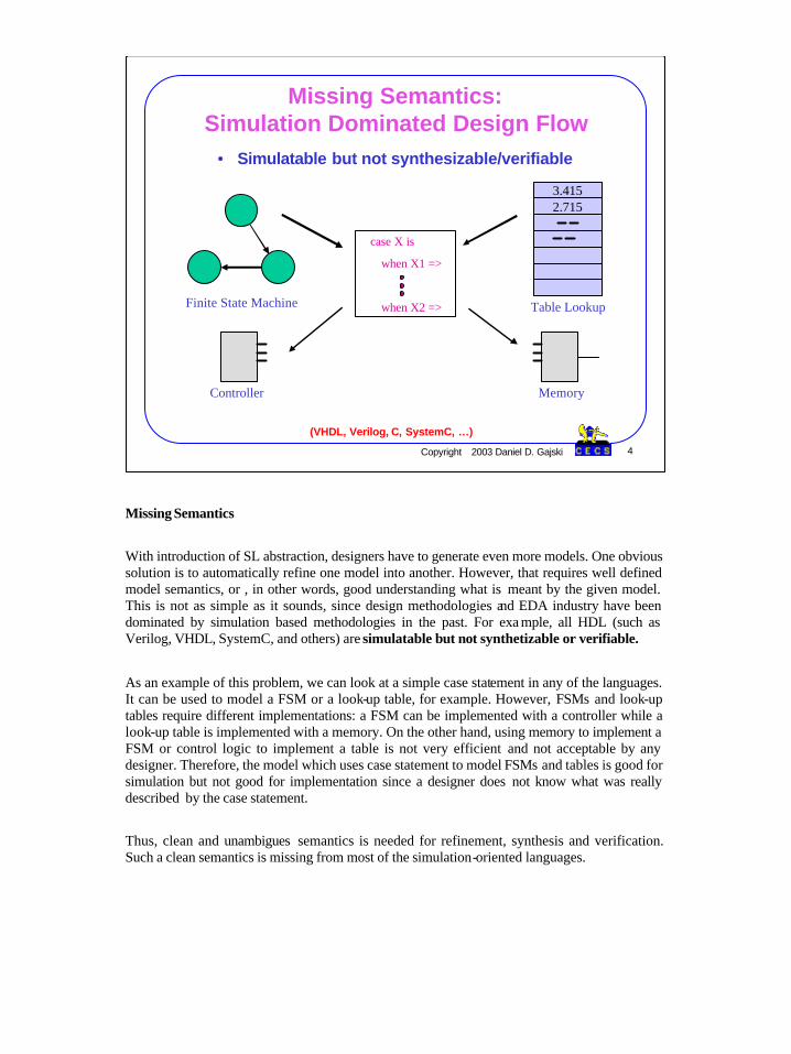
With introduction of SL abstraction, designers have to generate even more models. One obvious solution is to automatically refine one model into another. However, that requires well defined model semantics, or , in other words, good understanding what is meant by the given model. This is not as simple as it sounds, since design methodologies and EDA industry have been dominated by simulation based methodologies in the past. For exa mple, all HDL (such as Verilog, VHDL, SystemC, and others) are simulatable but not synthetizable or verifiable.
As an example of this problem, we can look at a simple case statement in any of the languages. It can be used to model a FSM or a look-up table, for example. However, FSMs and look-up tables require different implementations: a FSM can be implemented with a controller while a look-up table is implemented with a memory. On the other hand, using memory to implement a FSM or control logic to implement a table is not very efficient and not acceptable by any designer. Therefore, the model which uses case statement to model FSMs and tables is good for simulation but not good for implementation since a designer does not know what was really described by the case statement.
Thus, clean and unambigues semantics is needed for refinement, synthesis and verification.Such a clean semantics is missing from most of the simulation-oriented languages.
5
Copyright 2003 Daniel D. Gajski 5
Principles of Design Methodology
• Well defined specification• Specification is just a model without
implementation details• Complete, but it can be changed later
• Well defined system models• Several possible models• Well defined semantics • Formal representation
• Design synthesis• Design decisions => transformations• Automatic model generation
• Model verification• Formally defined transformations• Provable equivalence
System Specification model
Intermediate models
Cycle accurate implementation model
SER
Methodology Principles
In any design flow we need several models with emphasis on different design aspects and design details. A system level methodology starts with a well defined executable specification model that serves as the golden reference. The specification is gradually refined to a cycle accurate model that can be fed to traditional simulation and synthesis tools. The gradual refinement produces some intermediate models depending on the choice of methodology. It is important that these models are well defined with well defined semantics for each model.
The details that are added to models during refinement depend on the designer decisions. Each decision corresponds to one or more model transformations. If all the transformations are formally defined, the refinement process can be automated.
Furthermore, such a formalism leads to automatic verification . Since models and transformations are formally defined and transformations preserve equivalence then the equivalence of the original and refined models are easily established.
6
Copyright 2003 Daniel D. Gajski 6
Modeling as Algebra
• Algebra = < {objects}, {operations} >Set of all possible expressions [ex: a * (b + c)]
• Model Algebra = < {objects}, {compositions} >Set of all possible models [ex: ]
• Model Transformation t is a change in objects or composition
• Model refinement is an ordered set of transformations
• Methodology is a sequence of models and corresponding refinements
Model Algebra
Model algebras are based on similar concepts used in number algebras. An algebra is a set of objects and a set of operations. Objects can be a set of integers and operations can be + and *. Then the algebra defines the set of all possible expressions connected by + and *. Such an expression is a*(b + c).
Model algebra is a set of objects and a set of composition rules to combine those objects into larger objects. In case of well known FSM model, objects are states and composition rules are conditional arcs indicating the next state. For example FSM algebra represents all possible FSM models.
Model transformation is a change in objects or composition of a particular model. A sequence of transformations is called a refinement. While transformations are small and not significant changes in a model, a refinement, on the other hand, modifies the model dramatically by exposing a different aspect or characteristic of the design.Each design flow can be represented by a particular methodology which can be defined by a sequence of models and the sequence of corresponding refinements that transform one model in the sequence into another.
7
Copyright 2003 Daniel D. Gajski 7
Model Definition
• Model Algebra = < {objects}, {composition rules} >• Set of all possible models
• Objects• Behaviors (representing tasks / computations / functions)• Channels (representing communication between behaviors)• Components (processors, memories, buses, IPs)
• Relations• Relations define a specific model [a*((b+c)*(b-c))] • Relations define the model structure (composition and connectivity)
• Relation (cr n) ? {objects} x {objects}
Model Definition
Formally, a model is a set of objects and a set of composition rules defined on those objects. A specification level model would have objects like behaviors for computation and channels for communication, while an architecture model would have components such as processors, memories, IPsfor computation and buses for communication.
Composition rules combine objects into larger objects and create hierarchical structures.
Such a model algebra represents the set of all possible models that use the same set of objects and composition rules. Obviously, such a set of all possible models is infinite. A specific model is defined by a set of relations (one relation per each composition rule) which define which objects are related by the particular composition rule in the given model.
8
Copyright 2003 Daniel D. Gajski 8
Model Transformations (Rearrange and Replace)
• Rearrange composition of objects• Distribute execution across components
• Replace objects• Import library components
• Add / Remove synchronization• Transform a sequential composition to
parallel and vice-versa
• Decompose abstract data structures for communication• Execute data transaction over a bus
• Other transformations …
Source: Gajski,Abdi; Verify2003 Keynote
a*(b+c) = a*b + a*cDistributivity of multiplication
over addition
B2 B3
B1 B1
B2B3=
Distribution of behaviors (tasks)over components
analogous to……
PE1 PE2
Model Transformations
A transformation of a model can be viewed as a rearrangement or replacement of objects. For instance, in order to distribute the behaviors in a specification model across components in the system architecture model, we need to rearrange the behaviors into groups. Similarly, in order to refine communication over abstract channels to communication over system buses, we need to replace abstract channels with protocol channels. Another example of a transformation is a replacement of sequential with concurrent execution and adding synchronization to insure that the proper data values are used every time. Yet another example is decomposition of data for transmission over a limited capacity bus on the sender side and data assembly on the receiver side.
Intuitively, we can draw an analogy between distributive law for natural numbers and on the sender side distribution of behaviors over processing elements (PEs) as shown in the figure. Just as the expression on LHS of the equation is equal to that on RHS by rule of distributivity, the model on the LHS is equal to the model on the RHS by law of concurrent distribution. The equality of two models is determined by the same values of all variables after the execution. The same values are guaranteed by the same data dependencies in both models.
9
Copyright 2003 Daniel D. Gajski 9
Model Refinement
• Definition• Ordered set of transformations < tm, … , t2, t1 > is a refinement
if and only if model B = tm( … ( t2( t1( model A ) ) ) … )
• Refinement derives a more detailed model from an abstract one• Specific sequence for each model refinement• Not all sequences are relevant
• Automatic model generation• Each transformation can be automated• Each refined model can be automatically generated
• Equivalence verification• Each transformation maintains functional equivalence• Refinement is thus correct by construction
Model Refinement
A model refinement can be defined as a specific sequence of transformations. Usually, the refined model has more detail or a new feature. On the other hand, not every sequence of transformations is a relevant transformation.
If each transformation is well defined as an rearrangement or replacement, then model transformations can be automated. Similarly, refinements can be generated automatically. Furthermore, if each transformation is shown to be correct, the refinement will also produce a model equivalent to the original model.
10
Copyright 2003 Daniel D. Gajski 10
Refinement based Methodology
• Refinement based system level methodology• Methodology := < {models}, {refinements} >
• Each refinement is uniquely defined• Each refinement can be automated• No need for designer to write models• No need for different modeling languages• Designers only make design decisions
Refinement- based methodology
Any design flow or design methodology can be described by a set of models and the corresponding set of refinements of one model into another. Since each model refinement is well defined sequence of transformations, each refinement can be automated. If each refinement is automated, then each model can be automatically generated. If models are automatically generated then designers do not need to write different design models except the original specification model. If designers do not write models then there is no need for different modeling languages. In other words , designers only make design decisions, while every design decision is automatically applied through corresponding model transformation.
11
Copyright 2003 Daniel D. Gajski 11
System Synthesis through Refinement
• Set of models• Each design decisions => one model transformation
• Design is a sequence of decisions • Refinement is a sequence of model transformations• Synthesis = design + refinement• Challenge: define the design and refinement
sequences for each application
System Synthesis
Synthesis is the process of converting the functional description of a black box into a structure of the black box that consists of connected components from a given library. During this process we must make several different design decisions such as selecting components and their connectivity, mapping computation and communication constructs to components, ordering or scheduling computations or communications of different messages, adding new objects, insert ing synchronization to preserve dependences to name the few. The design process is a sequence o f such design decisions. Since for every design decision there is a model transformation, a sequence of design decisions will result in a sequence of transformations or model refinement. Therefore, synthesis is design plus refinement.
The main challenge for every application today is to define the appropriate set of models and corresponding refinements, and , furthermore, for every refinement, the sequence of design decisions and corresponding model transformations.
12
Copyright 2003 Daniel D. Gajski 12
System Verification through Refinement
• Set of models• Transformations preserve equivalence
• Same partial order of tasks• Same input/output data for each task• Same partial order of data transactions• Equivalent replacements
• All refined models will be “equivalent” to input model
Still need to verifyFirst specification modelCorrectness of replacements
Source: Gajski,Abdi; Verify2003 Keynote
RefinementTool
t1t2…tm
Model A
Model B
DesignerDecisions
Library ofobjects
System Verification
In a refinement based system-level methodology, each model produced by an automatic refinement is equivalent to the input model. As shown in the figure, designer decisions are used to add details to a model to refine it to the next lower level of abstraction. Each designer decision corresponds to a transformation in the model and each transformation preserves the equivalence of the model.
The notion of model equivalence comes from the simulation semantics of the model. Two models are equivalent is they have the same simulation results. This translates to the same (or equivalent) objects in both models, the same partial order of execution of tasks, same input and output data for each task and same partial order of data transactions. In other words, all data dependences must be preserved.Correct refinement, however, does not mean that the output model is bug free. We also need to use traditional verification techniques on the starting specification model and prove equivalence of objects that can be replaced with each other.
13
Copyright 2003 Daniel D. Gajski 13
Y Chart
Behavior(Function)
Structure(Netlist)
Physical(Layout)
Logic
Circuit
Processor
System
MoC
MoC
MoC
MoC
Y-Chart
In order to demonstrate the refinement-based methodology on the system level, we will start with the Y-Chart. It makes the assumption that each design, no matter how complex, can be modeled in three basic ways that emphasize different properties of the same design. Therefore, Y-Chart has three axes that represent design behavior (function, specification), design structure (netlist, block diagram), and physical design (layout, boards, packages). Behavior represents a design as a black box and describes its outputs in terms of its inputs and time. The black-box behavior does not indicate in anyway how to implement the black box or what its structure is. That is given on the structure axis, where black box is represented as a set of components and connections. Although, behavior of the black box can be derived from its component behaviors such behavior may be difficult to understand. Physical design adds dimensionality to the structure. It specifies size (height and width) of each component, the position of each component, each port and each connection on the silicon substrate or board or any other container. Y-Chart can also represent design on different abstraction levels identified by concentric circles around the origin. Each abstraction level uses different time granularity. Usually, four levels are identified: Circuit, Logic, Processor and System levels. The abstraction level can be also identified by the main component used in the structure. Thus, the main components on Circuit level are N or P-type transistors, while on Logic level they are gates and flip-flops. On the Processor level the main components are storage units such as register files and functional units such as ALUs, while on the System level they are processors, memories and buses. Converting behavior into structure on each abstraction level is called synthesis, and the structure into layout is called physical design. Every design methodology uses the bas ic models on the Y-Chart in addition to some intermediate models on the abstraction circles. Each abstraction level needs also a database of components on this level. Each component in the database has tree models representing three different axes in the Y-Chart: behavior or function (sometimes called Model of Computation (MoC)), structure of components from the lower level of abstraction and the physical layout or implementation of the structure. These components are IPs for each abstraction level.
14
Copyright 2003 Daniel D. Gajski 14
Processor (RTL) Behavioral Model
• Finite State Machine with Data (FSMD)• Combined model for control and computation
– FSMD = FSM + DFG
• Implementation: controller plus datapath
FSMD model (SFSMD model)
S1 S2
S3
Op2 Op3
Op4
Op6
Op1
Op5Op1 Op2
Op3
Op1 Op2
Processor Behavioral Model
The Processor behavioral or functional model is given by a Finite-state-machine with Data (FSMD). It combines finite-state-machine (FSM) model for control and data-flow-graph (DFG) for computation. FSM has a set of states and a set of transitions from one state into other depending on the value of some of the input. In each state FSMD executes a set of expressions represented by a DFG. FSMD model is clock-accurate if each state takes a single clock-cycle. On the other hand, if each DFG takes several clock cycles then the model is called Super FSMD (SFSMD). SFSMD and FSMD models can be used to represent any processor type including CISC, RISC, NISC and RTL processors.
It should be noted that FSMD model encapsulates the definition o f the state-based (Moore -type) FSM in which the output is stable during duration of each state. It also encapsulates the definition of the input-based (Mealy-type) FSM with the following interpretation: Input-based FSM transitions to a new state and outputs data conditionally on the value of some of FSM inputs. Similarly, FSMD executes set of expressions depending on the value of some FSMD inputs. However, if the inputs change just before the clock edge there may be not enough time to execute the expressions associated with that particular state. Therefore, designers should avoid this situation by making sure the input values change only early in the clock period or they must insert a state that waits for the input value change. In this case if the input changes too late in the clock cycle, FSMD will stay in the waiting state and proceed with a normal operation in the next clock cycle.
15
Copyright 2003 Daniel D. Gajski 15
• Multi-pipelined data path• Hardwired or programmable controller• RISC, NISC, or RTL style
Processor Structural Model
Bus1
Bus2
Bus3
Datapath
D Q
D Q
D Q
Controlinputs
Next-Sate
Logicor
Addressgenerator
Outputlogic
orProgrammemory
Stateregister
orPC
Controloutputs
Register
Selector
Register
Datapathoutputs
RFCache
ALU ∗ /÷
Signalstatus
Controller
Latch
Datamemory
IR
SR
Cotrolsignals
Processor Structural Model
The Processor structural model consists of a Datapath and a Controller.
The Datapath executes the DFG attached to each state in the FSMD model. The Datapath has storage units such as registers, register files, caches and memories, function units such as ALUs, multipliers, shifters, and connection units such as buses. Each unit may take one or several clock cycles to produce output. Furthermore, each unit can be pipelined through several stages. Furthermore each unit may have input and output latches or registers. Also each unit can be connected to any of the buses. The above flexibility can be used to pipeline the entire Datapath which comes useful when processing instruction streams in RISC/CISC processors or control streams in NISC/RTL processors.
The Controller keeps track of the presents state, defines the next state and controls the execution of the Datapath in each state. Its implementation defines the type of the processor. In case of a RTL processor (custom HW, IP), we have State register that stores the present state, Next -state logic (implemented with gates) that determines the next state, and output logic (implemented with gates) that defines the control signals for the simple Datapath (usually several registers and possibly an ALU). If FSMD is used to model NISC processor then Datapath is complex with multitude of storage units, functional units, and busses and heavily pipelined. In that case the controller has a PC instead of State register, Address generator instead on Next -state logic, and Programmable memory instead of Output-logic. This memory stores the control words for the Datapath, and Address generator generates memory address for the next control word in case of a NISC processor. In case of a RISC processor the memory stores instructions. If instructions are stored in the Programmable memory then we usually insert a Instruction register (IR) to temporary store instructions before they are decoded into contro l words. In case of a CISC processor decoding is performed by a second level memory whose addresses are supplied by IR.
Similarly, we can introduce a Status register (SR) to temporary store the conditions for computing the next state/address. In this case we have standard processor pipeline: PC, IR, Datapath pipe, SR, and back to PC.
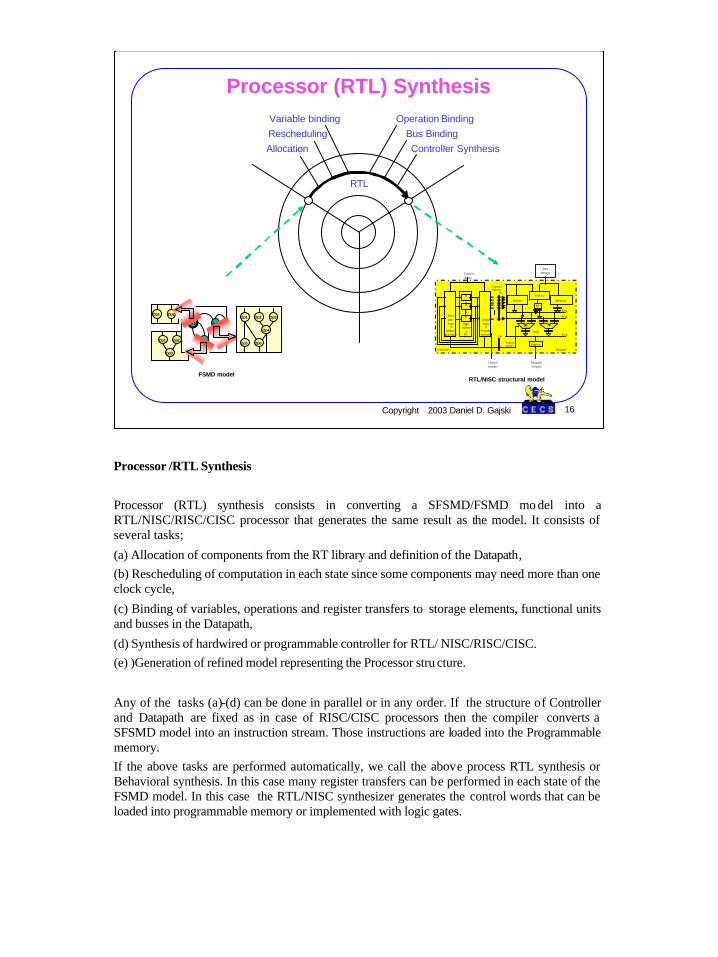
Processor (RTL) synthesis consists in converting a SFSMD/FSMD mo del into a RTL/NISC/RISC/CISC processor that generates the same result as the model. It consists of several tasks;
(a) Allocation of components from the RT library and definition of the Datapath,(b) Rescheduling of computation in each state since some components may need more than one clock cycle,
(c) Binding of variables, operations and register transfers to storage elements, functional units and busses in the Datapath,
(d) Synthesis of hardwired or programmable controller for RTL/ NISC/RISC/CISC.(e) )Generation of refined model representing the Processor stru cture.
Any of the tasks (a)-(d) can be done in parallel or in any order. If the structure of Controller and Datapath are fixed as in case of RISC/CISC processors then the compiler converts a SFSMD model into an instruction stream. Those instructions are loaded into the Programmable memory.If the above tasks are performed automatically, we call the above process RTL synthesis or Behavioral synthesis. In this case many register transfers can be performed in each state of the FSMD model. In this case the RTL/NISC synthesizer generates the control words that can be loaded into programmable memory or implemented with logic gates.
17
Copyright 2003 Daniel D. Gajski 17
System Functional Model
• Program State Machine– States described by procedures in a programming language
• Example: SpecC! (SystemC subset?!)
PSM modelProc
ProcProc
Proc
Proc
System Behavioral (Functional) Model
Since systems consists of many communicating components (processors, IPs) the FSMD model will not be able to model a system since it uses a single thread of execution.. The easiest way is to retain the concept of states and transitions as in a FSMD model but to extend the computation in each state to include one or more processes described in in a programming language such as C/C++. Furthermore, in order to represent an architecture with several processes running in parallel or in pipelined mode the system model should support concurrency (several components running in parallel) and pipelining (several components running in parallel with data passed between them sequentially). Since components are running concurrently we need a synchronization mechanism for data exchange. Furthermore, we need a concept of channel to encapsulate data communication. Also, we need to support hierarchy to allow humans to write easily complex systems specifications. Such a model is called Program State Machine (PSM).
System structural model consists of variety of system components such as processors, IPs, memories, arbiters and special application-specific custom hardware components (RTL processors). They can be connected through different connection components such as buses with specific bus protocols. In case that component and bus protocol do not match there must be specific Interface (IF) for connecting such components with incompatible protocols. In other words, system structural model a composition of system computation and connection components; any system can be modeled with such a model.
19
Copyright 2003 Daniel D. Gajski 19
System Synthesis
System
ProfilingAllocation IF Synthesis
Refinement
Behavior Binding Channel BindingVariable Binding
PSM model
Proc
Proc
Proc
Proc
Proc
Bus
System architecture
Memory
Memory
µProcessor
Interface
Comp.IP
Interface
Interface
Interface
Custom HW
System Synthesis
PSM model can be synthesized into a arbitrary system structure by the following set of tasks:
(a) Profiling of code in each behavioral model and collecting statistics about computation, communication, storage,traffic, power consumption, etc.,(b) Allocating components from the library of processors , memories , IPs and custom components/processors,
(c) Binding PSM processes to processing elements, variables to storage elements (local and global), and channels to busses,
(d) Synthesizing interfaces (IFs) between components and busses with incompatible protocols, and inserting arbiters, interrupt controllers, memory controllers, timers, and other special components.(e) Refining the PSM model into a architecture model that reflect allocation and binding decisions.
The above tasks can be performed automatically or manually. Tas ks (b)-(d) are usually performed by designers while tasks (a) and (e) are better done automatically since they require lots of mundane effort. Once the refinement is performed the structural model can be validated by simulation quite efficiently since all the component behaviors are described by high level functions.
In order to accomplish all the above tasks, we may use several intermediate models on the way to reach the system structural model from behavioral model.
20
Copyright 2003 Daniel D. Gajski 20
System Synthesis (continued)
RTL/IS Implementation+ results
Mem RFState
Control
ALU
Datapath
PC
Control Pipeline
IF FSM
IF FSMIP Netlist
RAM
IR
Memory
State
State
HCFSMD model
FMDS4
FSMD5
FSMD3
FSMD2
FSMD1
RTL MoC
System Synthesis (continued)
In order to generate cycle –accurate model, we must replace each component functional model with a FSMD/SFSMD model for RTL, NISC , RISC or CISC processors. Once we have cycle-accurate behavioral model, we can refine it further to cycle-accurate structural model by performing RTL synthesis for custom processors (custom IPs). On the other hand, behaviors assigned to standard processors we can compile into an instruction-set stream and combine it with a IS simulator (FSMD) to execute the compiled instruction stream. RTL synthesis can start from SFSMD that is obtained through two different mechanism. On one hand, we can replace a behavior assigned to an IP with a SFSMD model from IP library. On the other hand, we can perform RTL synthesis on any behavior assigned to a RTL processor after converting the behavior to a SFSMD by assigning each basic block to a super state. After RTL synthesis or behavior compilation for a standard processor we can easily generate a cycle-accurate model of the entire system.
21
Copyright 2003 Daniel D. Gajski 21
System Level Models
• Models based on time granularity of computation and communication• A system level design methodology is a path from model A to F
Computation
Communication
A B
C
D F
Un-timed
Approximate-timed
Cycle-timed
Un-timed
Approximate-timed
A. System specification modelB. Component -architecture model
C. Bus-arbitration modelD. Bus-functional modelE. Cycle-accurate computation model
F. Cycle-accurate implementation model
E
Cycle-timed
Source: Cai, Gajski. “Transaction level modeling: An overview”, ISSS 2003
System-level Models
In general, system level models can be distinguished by the accuracy of timing for their communication and computation. In the graph, the two axes represent the granularity of communication and computation. The functional specification at the origin is untimed, with only a causal ordering between tasks. On the other end of the spectrum is the cycle accurate model represented by the FSMD model.
A system level methodology takes the untimed specification to its cycle accurate implementation. The path through the intermediate models determines different types of refinements that must be performed.
22
Copyright 2003 Daniel D. Gajski 22
v2 = v1 + b*b; v3= v1- b*b;
v1
v1 = a*a;
v2
v4 = v2 + v3;c = sequ(v4);
B1
B2
v3
B3
B4
B2B3
Computation
Communication
A B
C
D F
Un-timed
Approximate-timed
Cycle-timed
Un-timed
Approximate-timed E
Cycle-timed
A: “Specification Model”
Objects- Computation
-Behaviors- Communication
-Variables
Composition
- Hierarchy
- Order
-Sequential
-Parallel
-Piped
-States
- Transitions
-TI, TOC
- Synchronization
-Notify/Wait
Specification Model
Specification model is a untimed model consisting of objects and composition rules for building larger objects. The objects can be used for computation and communication. Computation objects are behaviors or processes in the PSM model while variables are used for communication of data between behaviors. Composition rules allow construction of larger objects by using hierarchical encapsulation, and ordering of objects in sequential, parallel , pipelined or state fashion. Transition are used to specify the condition for execution of different behaviors, while synchronizations are used to insure that data are available at proper times.
The example shows 4 behaviors combined in sequential and parallel fashion with variables used to communicate data between them.
23
Copyright 2003 Daniel D. Gajski 23
B: “Component-Architecture Model”
v2 = v1 + b*b; v3= v1- b*b;
v1
v1 = a*a;
v 2
v4 = v2 + v3;c = sequ(v4);
B1
B2
v3
B3
B4
B2B3
A
v3
v3= v1- b*b;B3
v4 = v2 + v3;c = sequ(v4);
B4
PE3
v2 = v1 + b*b;B2
PE2
v1 = a*a;
B1
PE1
cv2
cv12
cv11
Computation
Communication
A B
C
D F
Un-timed
Approximate-timed
Cycle-timed
Un-timed
Approximate-timed
E
Cycle-timed
Objects- Computation
- Proc- IPs- Memories
- Communication-Variable channels
Composition
- Hierarchy
- Order
-Sequential
-Parallel
-Piped
-States
- Transitions
-TI, TOC
- Synchronization
-Notify/Wait
Component-Architecture Model
This model has same composition rules but several new objects representing different components. Additional computation objects are Processing Elements (PEs) that include processors, IPs and memories while new communication objects are variable channels used for communication between PEs. Inside the PEs we can still use behaviors and variables since execution is sequential and running on one processor. Since each behavior has been assigned to a PE, we can easily estimate the time for execution of each behavior. On the other hand, channels have not been assigned to busses and therefore we can not estimate the communication time.
In the Bus-Arbitration model a new component for communication is added: bus channel. Several variable channels are assigned to the bus channel. Since bus channel transfers data from a set of PEs to another set of PEs , we must insert a new arbiter PE to determine bus priority between several competing channels. Since bus has been selected we can also estimate the communication time for each channel.
In bus-functional model a real protocol is inserted into bus channel. Therefore, bus channel becomes cycle-accurate. The rest of the model stays the same. The communication traffic can be now accurately estimated.
In this model computation behaviors or processes are refined into SFSMD or FSMD models. Computation in each is therefore cycle-accurate while communication is still abstract with approximate timing. Since communication and computation do not have the same time granularity, each PE is encapsulated into a wrapper that abstracts its cycle-accurate time to approximate time of the communication model.
1: master interface2: slave interface3: arb i tor in ter face
r e a d yack
address[15:0]data[31:0]
IPro
toc
olS
lav
e
ready
a c k
address[15:0]
data[31:0]
D
Computation
Communication
A B
C
D F
Un-timed
Approximate-timed
Cycle-timed
Un-timed
Approximate-timed
E
Cycle-timed
Objects- Computation
- Proc- IPs (Arbiters)- Memories
- Communication-Buses (wires)
Composition
- Hierarchy
- Order
-Sequential
-Parallel
-Piped
-States
- Transitions
-TI, TOC
- Synchronization
-Notify/Wait
Cycle-Accurate Implementation Model
This model has cycle-accurate time in both computation and communication. Furthermore, the abstract bus channel is replaced with bus wires, while its functionality is unlined into PEs. In addition channel functionality is converted into FSMD model and combined with computational FSMD model.
28
Copyright 2003 Daniel D. Gajski 28
SoC Environment
Specification model
Architecture modelEstimation
Profiling
Profiling data
Design decisions
Communication model
Profiling weights
Arch. synthesis
Arch. refinement
Comm. synthesis
Comm. refinement
RefinementUser Interface (RUI)
Estimation results
Design decisions
Estimation
Impl. synthesis
Estimation results
Design decisions CA refinement
CA model
Capture
RTL/RTOSattributes
ValidationUser Interface (VUI)
Protocolmodels
Comp. / IPattributes
Protocolattributes
Comp. / IPmodels
Compile
Test
Simulate
Verify
Simulate
Verify
Allocation
Beh. partitioning
Scheduling / RTOS
Protocol selection
Channel partitioning
Spec. optimization
Cycle scheduling
Protocol scheduling
System structure
Arbitration
SW/HW synthesis
Algorithm selection
Lang. Translators
EstimationRTL/RTOSmodels
Estimation results
Test
Simulate
Verify
Test
Simulate
Verify
SoC Environment (SCE)
The SCE includes tools for specification (model A), architecture (model B), communication (model D) and implementation (model F) generation and synthesis. All or any number of synthesis tools can be included. For example, if the architecture is fixed, such as in a platform design, the architecture synthesis tool can be omitted. Similarly, if only a standard bus is used, the communication synthesis is not required. Furthermore, if no custom processors (RTL or NISC) are needed, the implementation synthesis can be substantially simplified.
SCE consists of several tool groups for different design tasks. Validation tools simulate, verify and test each model. Model generation tools generate automatically each model after designers make design decisions. Estimation tools estimate design metrics in order to help designers make decisions. Data bases contain characteristics and models of available components. User interface tools display the metrics, available components and captured or generated models as well as design task menu's. Synthesis tools replace designer decisions with automatically made decisions for design and model optimization and refinement.
29
Copyright 2003 Daniel D. Gajski 29
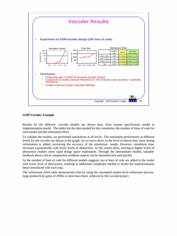
• Experiment on GSM Vocoder design (10K lines of code)
• Conclusion• Productivity gain >2,000X for industrial strength designs• Compare 9-12 months (manual refinement) vs. 50+4 minutes (user decisions + automatic
Results for the different vocoder models are shown here, from system specification model to implementation model. The tables list the time needed for the s imulation, the number of lines of code for each model and the refinement effort.
To validate the models, we performed simulations at all levels. The simulation performance at different levels for the vocoder are shown in the graph. As we move down in the level of abstraction, more timing information is added, increasing the accuracy of the simulation results. However, simulation time increases exponentially with lower levels of abstraction. As the results show, moving to higher levels of abstraction enables more rapid design space exploration. Through the intermediate models, valuable feedback about critical computation synthesis aspects can be obtained early and quickly.
As the number of lines of code for different models suggests, mo re lines of code are added to the model with lower level of abstraction, resulting in additional complexity needed to model the implementation detail introduced with each step.The refinement effort table demonstrates that by using the automated system level refinement process, large productivity gains of 2000x or more have been achieved in the vocoderproject.
Results for the JPEG encoder models are shown here from system specification model to implementation model. The graphs shows the time needed for the simulation and the number of lines of code for each model for encoding of a 116x96 black-and-white image.
To validate the models, we performed simulations at all levels. As we move down in the level of abstraction, more timing information is added, increasing the accuracy of the simulation results. However, simulation time increases exponentially with lower levels of abstraction. As the results show, moving to higher levels of abstraction enables more rapid design space exploration. Through the intermediate multiprocessing model, valuable feedback about critical computation synthesis aspects can be obtained early and quickly.
As the number of lines of code suggests, refinement between models is minimal and is limited to the additional complexity needed to model the implementation detail introduced with each step.The refinement effort table shows that automated system level refinement process can achieve 2000 times productivity gains comparing manual refinement process in JPEG project.
31
Copyright 2003 Daniel D. Gajski 31
Conclusion
• New design flow paradigm based on SER methodology• Semantics before syntax (language does not matter)• Model algebra before semantics• System verification, synthesis, modeling simplified• SW = HW = computation is the inevitable truth• SCE offers more then 1000X productivity gain• General problem: Define models, refinements,
methodology for specific applications
Conclusion
We have presented in this talk basic principles of SER paradigm system-level methodology based on this paradigm. It is based on a set of well defined models and automatic refinements from one model to the other. Since models are generated automatically, modeling languages do not matter. What matters is the semantics of each model. In order to establish adequate set of models we used the concept of model algebra which in turn simplifies the processes of simulation, synthesis and verification. Such an approach removes the differentiation between SW and HW since models of SW and HW on the system levels are the same. SW and HW become just computation.
In order to verify our concepts we have built the prototype of System-on-Chip Environment (SCE) which demonstrated on several selected industrial examples that productivity gains of more than 1000X can be expected. Although the basic principles h ave been proven to be correct, the main challenge in the future is the definition of application specific methodologies. In other words, the set of appropriate models, design decisions, transformations and refinements must be determined that fir a specific application.
32
Copyright 2003 Daniel D. Gajski 32
References
Gajski, Abdi; System Debugging and Verification: A New Challenge, Verify2003 Keynote, CECS TR 03-31, 2003 (www.cecs.uci.edu)
Cai, Gajski; Transaction Level Modeling: An Overview, Proc. ISSS, 2003, (www.cecs.uci.edu/~gajski/)
Gerstlauer et al; System Design, Kluwer Academic Publishers 2001