SYSTOLIC ARRAYS FOR MULTIDIMENSIONAL DISCRETE TRANSFORMS Weicheng Shen Martin Marietta Laboratories Baltimore, MD 21227-3848 A. Yavuz Oru¸c Electrical Engineering Department University of Maryland College Park, MD 20740 Submitted in April 1989 Revised in April 1990 ABSTRACT An active area of research in supercomputing is concerned with mapping certain finite sums, such as discrete Fourier transforms, onto arrays of processors. This paper presents systolic mapping techniques that exploit the parallelism inherent in discrete Fourier transforms. It is established that, for an M-dimensional signal, parallel executions of such transforms are closely related to mappings of an (M+1)-dimensional finite vector space into itself. Three examples of such parallel schemes are then described for the discrete Fourier transform of a two-dimensional finite extent sequence of size N 1 ×N 2 . The first is a linear array of N 1 +N 2 -1 processors and takes O(N 1 N 2 ) steps. The second is an N 1 ×N 2 rectangular array of processors and takes O(N 1 +N 2 ) steps, and the third is a hexagonal array which uses N 1 N 2 +(N 2 -1)(N 1 +N 2 -1) processors and takes O(N 1 +N 2 ) steps. All three mappings are optimal in that they achieve asymptotically highest speedup possible over the sequential execution of the same transform, and can easily be generalized to higher dimensions. 1
An active area of research in supercomputing is concerned with mapping certain finite sums, suchas discrete Fourier transforms, onto arrays of processors. This paper presents systolic mappingtechniques that exploit the parallelism inherent in discrete Fourier transforms. It is establishedthat, for an M-dimensional signal, parallel executions of such transforms are closely related tomappings of an (M+1)-dimensional finite vector space into itself. Three examples of such parallelschemes are then described for the discrete Fourier transform of a two-dimensional finite extentsequence of size N1×N2. The first is a linear array of N1+N2−1 processors and takes O(N1N2) steps.The second is an N1×N2 rectangular array of processors and takes O(N1+N2) steps, and the third isa hexagonal array which uses N1N2+(N2−1)(N1+N2−1) processors and takes O(N1+N2) steps. Allthree mappings are optimal in that they achieve asymptotically highest speedup possible over thesequential execution of the same transform, and can easily be generalized to higher dimensions.
1
1. Introduction
Certain finite sums such as discrete Fourier transforms (DFTs) find extensive applications in
many fields such as signal processing [Blahut 1985, Dudgeon and Mesereau 1984, Oppenheim
and Shafer 1984] pattern recognition [Blahut 1985, Jacobson and Wechsler 1984], computer
vision [Gafni and Zeevi 1979], computer arithmetic [Ling and Bayoumi 1988], and tomography
[Hinshaw and Lent 1983]. In most of these fields, one often deals with very large sets of discrete
signals which require more sophisticated techniques than conventional sequential transformation
schemes. For example, the fastest sequential DFT algorithm takes O(N logN) steps on a one-
dimensional, N-point array which should be iterated M times for a M-dimensional array, leading
to O(MNM logN) time complexity. While this order of complexity may be acceptable for small
values of N and M , certain design constraints such as the sampling rate and bandwidth of input
signals, often make it unacceptable to carry out discrete transforms on multidimensional signals
by sequential means.
For faster DFT computations, a number of parallel architectures have been proposed in the
literature [Cappello and Steiglitz 1983, Chakrabarti and Ja’Ja’ 1988, Chowdary et al. 1984,
Gertner and Shamash 1987, Miranker and Winker 1984, Zhang and Yun 1984]. [Thompson 83]
examined the VLSI complexity of one-dimensional DFTs using the area × time2 (AT 2) model
and surveyed several one-dimensional DFT algorithms. [Zhang and Yun 1984] presented a mesh-
connected processor array implementation of a two-dimensional DFT algorithm. [Chowdary et al.
1984] described a fast two-dimensional DFT processor. Recently, [Gertner and Shamash 1987]
introduced a hybrid architecture approach based on the well-known row-column decomposition
algorithm. They described two hybrid architectures, each using a butterfly array of processors
to perform a one-dimensional DFT and an interconnection network to reroute the intermediate
results back to the array between different phases of the algorithm. One of these architectures
uses a perfect shuffle network [Stone 1971] while the other uses what is called a rotation network
to align the outputs of the processor array between different phases of the computation. For an
N1×N2×. . .×NM array, where N1N2 . . .NM = N , the architecture with the rotation network achieves
AT 2 = (N2 log2N) which is optimal. More recently, [Chakrabarti and Ja’Ja’ 1988] generalized the
rotation network concept to obtain AT 2 optimal designs, but with other space and time tradeoffs.
While the designs in [Chakrabarti and Ja’Ja’ 1988, Gertner and Shamash 1987] meet the AT 2
lower bound for computing linear transforms, they require rotation networks with O(N21N
22 . . .N2
M )
area for an N1N2 . . .NM array of inputs. Moreover, these networks are difficult to layout in VLSI
[Franklin 1981]. To avoid the interconnection problems associated with these designs, this paper
examines three systolic implementations of the row-column decomposition algorithm within the
2
context of a program graph contraction procedure which was described in [Shen and Oruc 1989].
Such implementations have been described for other algorithms in the literature [Leiserson 1981,
Kung and Leiserson 1980]. The systolic arrays given in this paper extend these implementations
to the row-column decomposition algorithm by using simple last-in/first-out (LIFO) memories for
the alignment of intermediate results. For an N1 × N2 data array, the first implementation uses
a linear array of N1 + N2 − 1 processors and takes O(N1N2) steps. The second implementation
employs an N1×N2 rectangular array of processors and takes O(N1 +N2) steps, and the third one
uses a hexagonal array of N1N2 + (N2 − 1)(N1 +N2 − 1) processors and takes O(N1 +N2) steps. All
three have asymptotically optimal speedup when compared with the sequential implementation
of the row-column decomposition algorithm. Moreover, these implementations directly generalize
to M-dimensional signals without sacrificing their optimality. It is also shown that these systolic
implementations are just three instances of a wide spectrum of optimal systolic contactions of
the row-column decomposition algorithm.
The rest of the paper is organized as follows. Section 2 describes the program graph model and
the contraction mapping procedure. Section 3 describes the program graph for the row-column
decomposition algorithm. In Section 4, the mapping procedure of Section 2 is used to obtain
systolic contractions of this program graph. Section 5 discusses the memory organization and
interconnections of the resulting processor arrays. In Section 6, the contractions of Section 4
are generalized to discrete transformations of finite extent multidimensional signals. The paper
is concluded in Section 7.
2. Approach
The processor arrays to be described subsequently are all derived from systolic contractions of the
row-column decomposition algorithm [Dudgeon and Mersereau 1984]. Before we describe these,
it is first necessary to outline the main elements of our contraction procedure.
The procedure begins with a labelled program graph representation of the row-column decom-
position algorithm. Such representations, which have been used in the literature [Cytron 1988,
Ramakrishnan et al. 1986, Ramakrishnan and Varman 1984] earlier, are captured by a directed
acyclic graph G =< V,E,D >, where (1) V is a set of vertices, each representing a computation
step (computation vertex), an external input (source vertex), or a result from computation (sink
vertex); (2) E is a set of directed edges which specify the dependences between the computation
vertices in V ; and (3) D is a set of delays assigned to the edges in E so that the delay d asso-
ciated with an edge (a, b) ∈ E indicates that the operation at vertex b is to be initiated precisely
d clock ticks after the initiation of the operation at vertex a. A program graph is mapped to a
processor array by partitioning its computation vertices into disjoint subsets and assigning each
3
d
a b c
zyx w
x y z
Q
P
P Q
w
Figure 1. Contraction of a program graph.
subset to a separate processor. Depending on the partition, this results in a processor array with
a particular topology which will be called a target array or a systolic contraction of that program
graph. Computations in each group of vertices are then carried out by the processor, to which
they are assigned, in a sequential order and at a uniform rate as regulated by a global clock. The
interconnections between processors are determined as follows. Whenever two computation ver-
tices are merged, all the edges between the two are deleted, and all incoming and outgoing edges
to these two vertices are reconnected to the resultant vertex without altering their orientations.
The duplicate edges between the resultant vertices are also deleted unless their orientations are
different. The delays to be assigned to the links between the processors in the target array are
determined by algebraically summing them to zero around each loop of oriented edges much like
the voltages of branches within a loop add up to zero in an electrical circuit. As we shall see
subsequently, satisfying these delay equations simultaneously leads to processor arrays with very
simple processing elements. The determined delay values are used to schedule the arrivals of the
inputs. The exact locations at which the inputs enter a target array are determined in part by
the manner in which the computation vertices are partitioned and assigned to the processors in
the target array. A more formal presentation of the mapping procedure is given in [Shen 1987,
Shen and Oruc 1989]; the following example provides a brief description.
Figure 1 depicts a program graph with four computation vertices, a, b, c, d. Partitioning them into
sets {a, b, c} and {d} results in the target array with two processors P and Q, also shown in the
figure. The computation vertices a, b, and c are assigned to processor P , and computation vertex
4
d is assigned to processor Q. These assignments dictate that inputs x, y, and z enter processor P
in the order shown and with delay d1 between x and y, and delay d2 between y and z. On the
other hand, input w enters processor Q d3 clock ticks after y enters P to allow the required time
for the transmission of the data from processor P to processor Q along the link that connects the
two. Thus, a key constraint in assigning the computation vertices to processors and scheduling
the inputs for entry is that the processors fire their computations only when they have all of
their inputs available. Furthermore, processors have no decision capability, implying that they
repeatedly execute the same computation without knowing what their inputs are. All they know
is that they must compute whatever they see at their inputs at predetermined beats of time, for
example, t=1 second., t=3 seconds, t=5 seconds and so on. When a program graph does not
contain any loops of oriented edges, this constraint can easily be enforced by assigning each link
the minimum delay it can tolerate. When it does, we assign the delays to the links by summing
the delays to zero around each loop of oriented edges and simultaneously satisfying the resulting
equations.
In the following sections this procedure will be used to synthesize three systolic contractions of
the row-column decomposition algorithm.
3. The Row-column Decomposition Algorithm
In its most general form, the DFT of an M-dimensional sequence, x(n1, n2 . . . ,
nM ), is expressed as [Dudgeon and Mersereau 1984]
y(k1, k2, . . . kM ) =∑
n1,n2,...,nM
x(n1, n2, . . . , nM )Wn1k1N1
Wn2k2N2
. . .WnMkMNM
, (1)
where indicies ni, ki run over the domain [0, Ni − 1], 1 ≤ i ≤ M and WnikiNi
= exp(−j 2πnikiNi
) are
complex exponentials.
Several fast algorithms are known for efficiently computing this weighted sum. Among them, the
row and column decomposition algorithm is highly modular, that is, one can compute the DFT
of an M-dimensional signal by carrying it out M times over the indices nM , nM−1, . . . , n2, n1 in an
iterative manner. For example, if M = 2, then
y(k1, k2) =∑
0≤n1≤N1−1
∑0≤n2≤N2−1
x(n1, n2)Wn2k2N1
Wn1k1N2
, (2)
or if we let
G(n1, k2) =∑
0≤n2≤N2−1
x(n1, n2)Wn2k2N2
, (3)
then
y(k1, k2) =∑
0≤n1≤N1−1
G(n1, k2)Wn1k1N1
. (4)
5
Thus we can compute y(k1, k2) in two steps: First compute Equation (3), then compute Equa-
tion (4). Although both sums are computable, they are not in the best form to evaluate since
we need to simplify the weights Wn1k1N1
and Wn2k2N2
, that is, compute n1k1 mod N1 and n2k2 mod N2
when n1k1 ≥ N1, and n2k2 ≥ N2. This problem can be avoided if we use Horner’s rule of summation
and rewrite these sums recursively as given below:
algorithm. It will be assumed that these weights are precomputed and stored in a memory device.
This way, they can be accessed directly without any address computation since we need not
compute n1k1 mod N1 and n2k2 mod N2 anymore. This assumption is not unreasonable given that
a storage device with O(N1 +N2) words should suffice, and that the original problem size, N1N2,
is an order of magnitude greater than O(N1 + N2). In view of this assumption, the row-column
decomposition algorithm for a two-dimensional DFT requires N1N22 multiply-add operations for
the first phase, and N21N2 for the second phase, a total of N1N2(N1 +N2) steps.
These formulas generalize to M dimensions in a straighforward way; the DFT of a N1×N2×. . .×NMsample can be computed using the row-column decomposition algorithm in N1N2 . . .NM (N1 +N2 +
. . . +NM ) multiply-add steps. If N1 = N2 = . . . = NM = N, then the total number of multiply-add
operations becomes MNM+1. It should be noted that, from Equation (1), the direct computation
of an M-dimensional DFT needs (M + 1)N2M steps (NM additions and MNM multiplications
for each of the NM instances of the M-tuple k1k2 . . . kM). Thus, the row-column decomposition
6
method reduces the total number of steps by a factor of O(NM−1), which is considerable. However,
this is still too slow for large values of M , and we need to resort to parallel schemes.
The parallel schemes we shall describe in subsequent sections are based on systolic processor
arrays [Kung and Leiserson 1980]. To map the row-column decomposition algorithm on a systolic
array, we first represent each phase of the algorithm by a program graph, as shown in Figure 2.
and complex exponentials W k1N1, 0 ≤ k1 ≤ N1 − 1, respectively. The horizontal lines represent the
final sums y(k1, k2), which are the desired results. Observe that the program graphs in Figure 2(a)
and 2(b) each represent a one-dimensional DFT. In general, the DFT of an M-dimensional input
can be represented by M program graphs where the first graph describes the one-dimensional
DFT of the input along the first axis, the second graph describes the one-dimensional DFT along
the second axis, and so on.
4. Row-column Decomposition on Systolic Arrays
This section describes how to map the program graph given in Section 3 on three systolic arrays
with linear, rectangular, and hexagonal geometries. In each case, we will establish that the given
design asymptotically achieves the highest speed up possible, and therefore, is asymptotically
optimal. These designs will later be extended to M-dimensional transforms in Section 6.
Linear Array Implementation
First, consider the linear array implementation. By starting out with the program representation
of the row-column decomposition algorithm, we can obtain a linear processor array by grouping
the computation vertices which fall on the vertical lines as shown in Figure 3. For an N1 × N2
sequence, this results in a linear array with N1 + N2 − 1 processors as illustrated in Figure 4 for
N1 = N2 = 3. The processors are labelled Pi, 0 ≤ i ≤ N1 + N2 − 2 where P0 denotes the rightmost
processor and PN1+N2−2 denotes the leftmost processor.
7
x(0,2) x(0,1) x(0,0)
x(1,2) x(1,1) x(1,0)
x(2,2) x(2,1) x(2,0)
G (0,0)0
G (0,1)0
G (0,2)0
G (0,0)3
G (0,1)3
G (0,2)3
G (1,0)0
G (1,1)0
G (1,2)0
G (1,0)3
G (1,1)3
G (1,2)3
G (2,0)0
G (2,1)0
G (2,2)0
G (2,0)3
G (2,1)3
G (2,2)3
G(2,2) G(1,2) G(0,2)
G(2,1) G(1,1) G(0,1)
G(2,0) G(1,0) G(0,0)
y (0,2)0
y (1,2)0
y (2,2)0
y (0,2)3
y (1,2)3
y (2,2)3
y (0,1)0
y (1,1)0
y (2,1)0
y (0,1)3
y (1,1)3
y (2,1)3
y (0,0)0
y (1,0)0
y (2,0)0
y (0,0)3
y (1,0)3
y (2,0)3
Phase 1
Phase 2
a
b c
ac+b
bc
Computation at each vertex
W03
W13W
23
W03
W13
W23
W03
W13W
23
W03
W13
W23
W03
W13W
23
W03
W13
W23
Figure 2. A program graph for the row-column decomposition algorithm.
8
x(0,2) x(0,1) x(0,0)
x(1,2) x(1,1) x(1,0)
x(2,2)x(2,1) x(2,0)
G (0,0)0
G (0,1)0
G (0,2)0
G (0,0)3
G (0,1)3
G (0,2)3
G (1,0)0
G (1,1)0
G (1,2)0
G (1,0)3
G (1,1)3
G (1,2)3
G (2,0)0
G (2,1)0
G (2,2)0
G (2,0)3
G (2,1)3
G (2,2)3
G(2,2) G(1,2) G(0,2)
G(2,1) G(1,1) G(0,1)
G(2,0) G(1,0) G(0,0)
y (0,2)0
y (1,2)0
y (2,2)0
y (0,2)3
y (1,2)3
y (2,2)3
y (0,1)0
y (1,1)0
y (2,1)0
y (0,1)3
y (1,1)3
y (2,1)3
y (0,0)0
y (1,0)0
y (2,0)0
y (0,0)3
y (1,0)3
y (2,0)3
Phase 1
Phase 2
W03
W13W
23
W03
W13
W23
W03
W13W
23
W03
W13
W23
W03
W13W
23
W03
W13
W23
d2
d1
d3
d5
d4
Loop
Figure 3. A contraction which results in a linear array.
The row-column algorithm is carried out by this array in two phases. In the first phase, all inputs
x(i, j) for which i+ j = k are fed into processor Pk in ascending row order, that is, the entries with
the smallest row index first, the entries with the next smallest row index next, and so on. This is
in keeping with the order among x(i, j) as established by the time paths of Figure 3(a). Moreover,
9
DPP
01234PPP
D DD
x(0,0)
x(0,0)
x(0,2)x(0,2)
x(0,2)
x(0,1)
x(0,1)
x(0,1)
x(0,0)x(1,0)
x(1,0)
x(1,0)
x(1,1)
x(1,1)
x(1,1)
x(2,0)
x(2,0)
x(2,0)
x(1,2)
x(1,2)
x(1,2)
x(2,1)
x(2,1)
x(2,1)
x(2,2)
x(2,2)
x(2,2)
G (0,1)
G (0,2)
G (1,0)
G (1,1)
G (1,2)
G (2,0)
G (2,1)G (2,2)
G (0,0)
0
0
0
0
0
0
0
0
0W3
W3
W3
W3
W3
W3
W3
W30
1
2
0
1
2
0
W31
2
G(i,j)'s exit here
DPP01234
PPPD DD
G(0,2)
G(0,2)
G(2,2)G(2,2)
G(2,2)
G(1,2)
G(1,2)
G(1,2)
G(0,2)G(0,1)
G(0,1)
G(0,1)
G(1,1)
G(1,1)
G(1,1)
G(0,0)
G(0,0)
G(0,0)
G(2,1)
G(2,1)
G(2,1)
G(1,0)
G(1,0)
G(1,0)
G(2,0)
G(2,0)
G(2,0)
y (1,2)
y (2,2)
y (0,1)
y (1,1)
y (2,1)
y (0,0)
y (1,0)y(2,0)
y (0,2)
0
0
0
0
0
0
0
0
0y(i,j)'sexit here
Phase 1
Phase 2
W3
W3
W3
W3
W3
W3
W3
W30
1
2
0
1
2
0
W31
2
Pi ac + bc ca
b
Figure 4. Row-column decomposition on a linear array.
each x(i, j) is fed into the array N2 times since each processor needs to execute N2 computation
vertices per each group of horizontal lines in the original program.
As a second group of entries, the weights W iN2, 0 ≤ i ≤ N1 − 1, enter the array through P0 and
proceed to the left at the same speed as x(i, j) but with N2−1 times the delay between consecutive
10
entries in x (twice for the processor array of Figure 4). The elements of G enter the array at
processor PN1+N2−1 and march to the right one clock tick at a time. The increase in the delays
between consecutive entries in the weight sequence is necessary for the correct timing of the
computations at the processors and is accomplished by the delay elements inserted between
consecutive processors. This can be seen by examining a loop of delays shown in heavy lines in
Figure 3. As stated in Section 2, for the target array to be systolic, the algebraic sum of the
delays in every loop of edges in the corresponding program graph must be zero. Using this fact
we can write for the loop shown in Figure 3(a)
d1 + d2 + d3 − d4 − d5 = 0. (5)
Furthermore, we let d1 = d2 = d3 = 1 in order to make the delays between the consecutive entries
in the x sequence equal. This then leads to
3− d4 − d5 = 0, (6)
which we can use to adjust the delays between the elements in the G(i, j) and Wn2N2
sequences. In
the linear array of Figure 4, we let d4 = 1 and d5 = 2 although it is possible to have other values
for d4 and d5 as long as this equation is satisfied. Also, note that for an N1 ×N2 input sequence,
Equation (6) generalizes to N2 − 1− d4 − d5 = 0.
The arrivals of the inputs at the processors in Figure 4 are scheduled to meet the delays determined
above. The elements of x are skewed as they enter the processors. Similarly, the elements of G are
also skewed N1 clock ticks as they enter the array through processor PN1+N2−1. The computations
in the second phase proceed similarly.
As for the time complexity, the total number of clock ticks to complete the first phase can be
computed directly from the arrivals of the inputs at the processor in the middle, that is, processor
PN2−1. It takes N1 +N2 − 1 clock ticks for the first input to arrive and thereafter N1N2 clock ticks
for the last input to arrive at this processor. At this time, the last element in the G sequence
also arrives at PN2−1 and needs N2 clock ticks to exit from the rightmost processor. Adding these
together, we have N1 + 2N2 − 1 +N1N2 clock ticks.
The second phase of the algorithm is identical to the first one, except that the G sequence
assumes the role of x, and y replaces G as output. The total time Tlinear to compute both phases
of the row-column decomposition algorithm on a linear array with N1 + N2 − 1 processors then
becomes
Tlinear = 2(N1N2 + 2N1 +N2 − 1). (7)
11
Let Slinear denote the speedup of the linear array over the sequential implementation of the
row-column decomposition algorithm. Since it takes N1N2(N1 + N2) steps to perform the same
algorithm on a single processor, we have
Slinear =N1N2(N1 +N2)
2(N1N2 + 2N1 +N2 − 1). (8)
If N1 = N2 = N , then
Tlinear = 2N2 + 6N − 2 (9)
and
Slinear =2N3
2N2 + 6N − 2= O(N). (10)
This is asymptotically optimal since a total of 2N − 1 processors is used.
The linear array described above is one of many arrays which can be obtained from the program
graph of Figure 2. As another possibility, suppose that we assign all the N1N2 computation vertices
within each horizontal block in Figure 2(a) to the same processor. This can easily be seen to
lead to a linear array with N1 processors. Likewise, by grouping the computation vertices in each
horizontal block in Figure 2(b), we obtain a linear array with N2 processors. Similarly, when all
computation vertices in each diagonal block are assigned to the same processor, another linear
array may be obtained. A detailed discussion of these and other linear array implementations will
be deferred to another place. It suffices to say that these two implementations also result in a
linear speedup as in the linear array given in Figure 4.
Rectangular Array Implementation
While the linear speedup is the best possible for a linear array implementation of the row-
column decomposition algorithm, it only reduces the total computation time to O(N1N2) from
O(N1N2(N1 +N2)). More can be done by using arrays with O(N1N2) processors. To form such an
array, we must partition the computation vertices in the program graph in Figure 2 into roughly
O(N1×N2) processors. One possibility is as shown by the heavy lines in Figure 5 for N1 = N2 = 3.
In this case, each of the two phases of the algorithm is contracted along the antidiagonal paths
to obtain the rectangular arrays of processors shown in Figure 6. The number of processors is
N2 ×N2 for the first phase and N1 ×N1 for the second phase. When N1 = N2 = N , both phases
need N2 processors. As for the assignment of computation vertices to the processors, all com-
putation vertices on the i-th antidiagonal from the top left-hand corner where 0 ≤ i ≤ N1N2 − 1
are assigned to the processor in row 1 + bi/N1c and column i mod N2 in the target array. As can
be seen from Figure 6, only the entries of x and G matrices move in the first phase and similarly
only the entries of y and G move in the second phase. The weights are stored in registers local
12
x(0,2) x(0,1) x(0,0)
x(1,2) x(1,1) x(1,0)
x(2,2) x(2,1) x(2,0)
G (0,0)0
G (0,1)0
G (0,2)0
G (0,0)3
G (0,1)3
G (0,2)3
G (1,0)0
G (1,1)0
G (1,2)0
G (1,0)3
G (1,1)3
G (1,2)3
G (2,0)0
G (2,1)0
G (2,2)0
G (2,0)3
G (2,1)3
G (2,2)3
G(2,2) G(1,2) G(0,2)
G(2,1) G(1,1) G(0,1)
G(2,0) G(1,0) G(0,0)
y (0,2)0
y (1,2)0
y (2,2)0
y (0,2)3
y (1,2)3
y (2,2)3
y (0,1)0
y (1,1)0
y (2,1)0
y (0,1)3
y (1,1)3
y (2,1)3
y (0,0)0
y (1,0)0
y (2,0)0
y (0,0)3
y (1,0)3
y (2,0)3
Phase 1
Phase 2
W03
W13W
23
W03
W13
W23
W03
W13W
23
W03
W13
W23
W03
W13W
23
W03
W13
W23
Figure 5. A contraction which results in a rectangular array.
to the processors in both phases. Also from the figure, it is obvious that the delays between the
elements of x must be the same as the delays between the elements of G for the first phase, and
similarly, the delays between the elements of y and those between the entries of G must be the
same for the second phase. As for the arrivals of x and G matrices at the inputs of the array, it
13
x(2,0)
W3 W3 W3
W3 W3 W3
W3 W3 W3
0 00
1 1 1
2 2 2
y(0,2)y(1,2)y(2,2)
y(0,1)y(1,1)
y(0,0)y(1,0)
y(2,1)
y(2,0)
G(2,2)
G(2,1)
G(2,0)
G(1,2)
G(1,1)G(1,0)
G(0,2)G(0,1)
G(0,0)
Phase 2
W3 W3 W3
W3 W3 W3
2W3 W3 W3
0 00
1 1 1
2 2
G(0,0)G(0,1)G(0,2)
G(1,0)G(1,1)G(1,2)
G(2,0)G(2,1)G(2,2)
x(0,2)
x(1,2)
x(2,2)
x(0,1)
x(1,1)
x(2,1)
x(0,0)
x(1,0)
Phase 1
Computation at each processorb
a
b
W3i
b+api,j
Figure 6. Row-column decomposition on a rectangular array.
is easily seen that they need to be skewed as shown in Figure 6 to achieve the correct timing of
computations at the processors.
With these facts, it takes 2N1 − 1 +N2 steps to complete the first phase, and 2N2 − 1 +N1 steps
14
to complete the second phase, and hence
Trectangular = 3(N1 +N2)− 2 (11)
steps to run the overall algorithm on an N2×N2 rectangular array of processors for the first phase
and an N1 ×N1 rectangular array of processors for the second phase. It follows that the speedup
over the single processor implementation is
Srectangular =N1N2(N1 +N2)3(N1 +N2)− 2
. (12)
If we assume N1 = N2 = N , then
Trectangular = 6N − 2 (13)
and
Srectangular =2N3
6N − 2= O(N2). (14)
This again is asymptotically optimal as in the linear processor array case since a total of N2
processors is used.
Another rectangular array implementation can be obtained by mapping each row of computation
vertices to a different processor. In this case the horizontal inputs, –entries of G matrix in the
first phase, and those of y matrix in the second phase– must be made stationary and stored
in local memories of the processors. This, obviously, doubles the memory space needed by the
earlier solution when N1 = N2 = N , since the earlier solution needs to store only the weights W i,jN
for both phases of the algorithm.
Hexagonal Array Implementation
To implement the row-column decomposition algorithm on a hexagonal array of processors, we
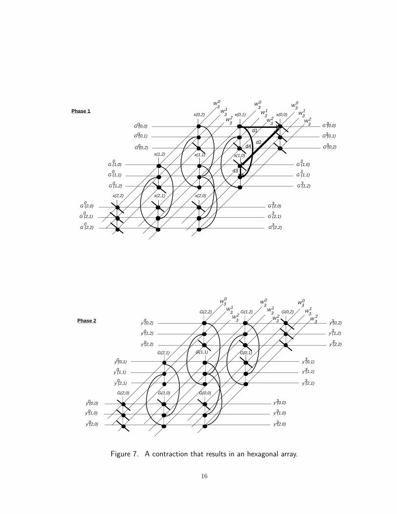
partition the computation vertices as shown in Figure 7 for N1 = N2 = 3. The resulting graph
can then be contracted into a processor arrray (see Figure 8). It should be obvious that after
the contraction, each processor vertex ends up having six distinct adjacent neighbors and thus
can be modelled as a hexagonal cell. It can also be verified that the target array contains
N1N2 + (N2− 1)(N1 +N2− 1) processors for the first phase and N1N2 + (N1− 1)(N1 +N2− 1) for the
second phase. When N1 = N2 = N , both processor counts reduce to 3N2 − 3N + 1.
Now, to describe which computation vertex is mapped to which processor, consider the αth
column of computation vertices where 0 ≤ α ≤ N1 +N2 − 1 in either graph in Figure 7. These can
be partitioned into some β N2×1 column matrices where 0 ≤ β ≤ N1−1. Let these column matrices
be denoted by Ck, 0 ≤ k ≤ β−1 where C1 is the top most matrix, C2 is the next topmost matrix and
15
x(0,2) x(0,1) x(0,0)
x(1,2) x(1,1) x(1,0)
x(2,2) x(2,1) x(2,0)
G (0,0)0
G (0,1)0
G (0,2)0
G (0,0)3
G (0,1)3
G (0,2)3
G (1,0)0
G (1,1)0
G (1,2)0
G (1,0)3
G (1,1)3
G (1,2)3
G (2,0)0
G (2,1)0
G (2,2)0
G (2,0)3
G (2,1)3
G (2,2)3
Phase 1
G(2,2) G(1,2) G(0,2)
G(2,1) G(1,1) G(0,1)
G(2,0) G(1,0) G(0,0)
y (0,2)0
y (1,2)0
y (2,2)0
y (0,2)3
y (1,2)3
y (2,2)3
y (0,1)0
y (1,1)0
y (2,1)0
y (0,1)3
y (1,1)3
y (2,1)3
y (0,0)0
y (1,0)0
y (2,0)0
y (0,0)3
y (1,0)3
y (2,0)3
Phase 2
W03
W13W2
3
W03
W13W2
3
W03
W13W2
3
W03
W13W2
3
W03
W13W2
3
W03
W13W
23
d1
d2d4
d3
Figure 7. A contraction that results in an hexagonal array.
16
G(2
,2)
x(0,2)
x(1,1)
x(2,0)
x(0,1)
x(1,0)
x(0,0)x(1,2)
x(2,1)
x(2,2)
G(0
,0) G(1
,1)
G(0
,1) G(1
,2)
G(0
,2)
G(2
,0)
G(2
,1)
G(1
,0)
W 3 W
3 P0,2
P0,3
P0,4
P1,4
P2,4
P0,0
P0,1
P1,0
P1,1
P1,2
P1,3
P2,0
P2,1
P2,2
P2,3
P3,1
P3,2
P3,3
P4,2
Phase 1y(
2,0)
G(2,2)
G(1,1)
G(0,0)
G(1,2)
G(0,1)
G(0,2)G(2,1)
G(1,0)
G(2,0)
y(0,
2) y(1,
1)
y(1,
2) y(2,
1)
y(2,
2)
y(0,
0)
y(1,
0)
y(0,
1)
P0,2
P0,3P0,4
P1,4
P2,4
P0,0
P0,1
P1,0
P1,1
P1,2
P1,3
P2,0
P2,1
P2,2
P2,3
P3,1
P3,2
P3,3
P4,2
Phase 2
W 3 W
3 0
W 3
2
W 3 0
W 3 0
1
1
W 3
2
W 3
2
1
Computation at each processor
Pi,j
bc
a c
ac+b
b
W 3 W
3 0
W 3
2
W 3 0
W 3 0
1
1
W 3
2
W 3 2
1
W 3 W
3
Figure 8. Row-column decomposition on a hexagonal array.
so on. Let C = [CT1 CT2 ...C
Tα ]. Then all computation vertices on each antidiagonal of C are mapped
to the same processor in the target array. More specifically, let P0,α, P1,α, ..., Pβ+N2−1,α denote the
processor vertices in the αth column of the target array, where P0,α is the topmost processor
vertex, P1,α is the next topmost processor vertex, and so on. Then all computation vertices on
17
the ith antidiagonal of C from the top righthand corner are assigned to Pi,α, 0 ≤ i ≤ β +N2 − 1.
As in the earlier two cases, the row-column decomposition algorithm is executed in two phases.
During the first phase the hexagonal array computes a matrix of partial sums G by performing
a one-dimensional DFT with respect to index n2. During the second phase, a one-dimensional
DFT is performed on G with respect to index n1. Matrix y is then the desired two-dimensional
DFT of the input sequence x.
As for the time delays between the entries in the input and output sequences, consider the loop
shown in Figure 7(a). Given the orientations of the edges in the loop, we can write d1+d2+d3−d4 =
0. If we assume that the entries of the input, output, and weight sequences all move at the same
speed between the processors, we can let d1 = d2 = d3 = 1 which then implies d4 = 3. It follows
that the computations consecutively scheduled on each processor must be executed with three
delay units in between. This accounts for the delays between the entries of the input and output
sequences as shown in Figure 8. It can further be shown that the first phase of the algorithm
needs 3(N1 − 1) + 1 steps for the last entry in the G sequence, that is, G(N1 − 1, N2 − 1) to enter
the array, and N1 + N2 − 1 steps thereafter to move out along the main diagonal which adds up
to 4N1 + N2 − 3 steps. Similarly, the second phase takes 4N2 + N1 − 3 steps, and hence the total
number of steps is
Thexagonal = 5(N1 +N2)− 6, (15)
and the speedup over the single processor implementation is
Shexagonal =N1N2(N1 +N2)5(N1 +N2)− 6
. (16)
If N1 = N2 = N , then
Thexagonal = 10N − 6 (17)
steps overall, and
Shexagonal =2N3
10N − 6= O(N2). (18)
Even though the speedup in this case is worse than the speedup for the rectangular array in exact
terms, it is still asymptotically optimal since O(N2) processors are used. In fact, one can reduce
the constant multiplying N in Equation 17 by using other hexagonal array contractions of the
row-column decomposition algorithm. However, this does not change the asymptotic complexity
of such contractions which is O(N).
5. Alignment of Intermediate Results
In the last section, we described three processor arrays for the row-column decomposition al-
gorithm without discussing how to align the intermediate results between the two phases of
18
Wi
N1 Wi
N2enter here
MUX MUX MUX MUX MUX
x(i,j) x(i,j) x(i,j) x(i,j) x(i,j)
DMUX
LIF
O
LIF
O
LIF
O
LIF
O
Figure 9. Memory organization for the linear array implementation.
the algorithm. In most array processors, the data between successive phases of an algorithm
are aligned by an interconnection network placed between the system’s memory and processors
[Lawrie 1975, Stone 1971]. However, the three systolic arrays described above do not need such
a network, and as we discuss below, a simple LIFO memory is sufficient for aligning the data
between the two phases of the row-column decomposition algorithm.
First, consider the linear array implementation and, for simplicity of discussion, let N1 = N2 = N.
At the end of the first phase, the G sequence leaves the array as a single stream of outputs which
should be organized into a (2N − 1) × N matrix as it enters the array in the next phase. Notice
that the elements with distinct indices in each column are computed in reverse order in the first
phase and hence must be realigned for the second phase. A total of 2N − 1 LIFO memories,
each with N locations, can provide the desired alignment of the G sequence (see Figure 9). It is
possible to save some memory space by observing that not all processors need the same number
19
x(i,j) exit here in the first phaseG(i,j) exit in the second phase
G(i,
j) en
ter
here
in th
e fir
st p
hase
y(i,j
) en
ter
in th
e se
cond
pha
se
W03
W03
W03
W13
W13 W1
3
W23 W2
3 W23
MUX MUX MUX
x(i,j)x(i,j) x(i,j)
Figure 10. Memory organization for the rectangular array implementation.
of inputs, but this does not change the overall storage complexity of the solution, which is O(N2).
In addition, a demultiplexer is needed to select the right LIFO unit in storing the entries of G.
The control circuitry for moving the intermediate results back to the array through the LIFOs is
a simple exercise in sequential circuit theory and will not be presented here. It suffices to observe
that the data which leaves the array in the first phase is needed in the reverse order in the second
phase. To select between the x and G sequences for the vertical inputs in the two phases, we can
connect a multiplexer circuit to each vertical input of the array and multiplex these two sequences
as shown in Figure 9.
Next, consider the rectangular array implementation. This time the intermediate results become
available in parallel and hence can be stored simultaneously without using a demultiplexer circuit
20
as shown in Figure 10. However, note that the elements of G leave the array in the first phase
in reverse order as in the linear array case, and hence LIFO memories are needed in this case as
well. This time, however, we need only N LIFOs each with N locations.
Finally, for the hexagonal array, Figure 8 reveals that, as in the first two cases, the G sequence
computed in the first phase must be reversed before it enters the array for the second phase.
It can be seen that a total of 2N − 1 LIFOs, each with N locations, is sufficient to carry out
this alignment. Like the rectangular array, no demultiplexer is required since the results become
available simultaneously. It follows that the total storage complexity of this implementation is
the same as that for the linear array.
6. Extension of Results to Other Arrays and Higher Dimensions
So far we have discussed the processor array implementations of one and two dimensional DFTs.
It should be obvious that the mapping technique is not limited to these dimensions since the
contraction of the program graph and task scheduling are carried out for each phase separately,
and will be identical for all phases except that the inputs will be different. Thus for an M-
dimensional DFT, we use the same program graph and the same array –be it linear, rectangular,
hexagonal, or any other– with the same timing. The only part which is involved is the alignment
of intermediate results between the M phases of the algorithm. The key observation is that we
now have M summations whose operands must be multiplexed and permuted into the inputs
of a single target array. [Gertner and Shamash 1987] described a general scheme to align the
intermediate results by a rotation network which essentially transposes the intermediate results
between two consecutive phases. In our designs, we need not use such a network since the
transposition, or reversal of the outputs from one phase to the next phase, can be handled with
a minor modification of the LIFO memories used in the two-dimensional DFT scheme described
above. Rather than have a single LIFO for each vertical input, we now use a pair of LIFOs,
between which we alternate the data reversals and feeds. During a given phase, one will be filled
with the outputs from the array needed for the next phase, while the other feeds the vertical
input to which it is connected with the desired sequence of elements. In the next phase, the roles
of the two LIFOs are interchanged so that the one that was filled during the last phase will now
feed the data for the vertical input, and the other will be filled with the outputs needed for the
following phase. Obviously, this modification does not alter the overall order of complexity of the
alignment hardware, and the bounds which hold for the two-dimensional DFT case remain intact.
As for other processor array implementations of the row-column decomposition scheme, it should
be obvious from the examples given in Section 4 that one can contract the program graphs in
Figure 3 to many other processor arrays by defining other partitions of computation vertices.
21
We mentioned a few in Section 4, and many more arrays can be obtained. In general, we can
view the computation vertices of the corresponding program graph as a set S of all points in a
three-dimensional finite vector space, i.e., S = {(x, y, z) : x, y, zε{0, 1, . . . , N − 1}} which contains N3
points. With this representation, any contraction of the program graph can then be viewed as a
mapping of S into a set P of processors where |P | = |S|. For example, if P = {p1 : 0 ≤ i ≤ N3},then f : S → P defined by f(x, y, z) = pz projects all computation vertices on the z = 0 plane to
p0, those on the z = 1 plane to p1, and so on. This projection describes a contraction of the
original program graph to a linear array with N processors. Other processor arrays can be defined
similarly by using other maps from S to P . The total number of such maps can easily be shown
to be N3N3for a two-dimensional DFT, and more generally, N (M+1)NM+1
for an M-dimensional
DFT. It can also be shown that not all of these maps lead to systolic arrays, and characterization
of those which result in systolic arrays remains an interesting open problem.
7. Concluding Remarks
We have examined systolic contractions of multidimensional discrete Fourier transforms with a
particular focus on two-dimensional DFTs. It is established that for an M-dimensional DFT,
any such contraction can be represented by a mapping of an (M + 1)-dimensional finite vector
space into itself. In more specific terms, three such contractions leading to linear, rectangular,
and hexagonal processor arrays have been described. Each of these achieves asymptotically
optimal speed up over a single processor implementation, even though the linear array takes
O(N2) time with O(N) processors, and the other two take O(N) time with O(N2) processors. It
should be noted that these time complexities can be reduced to meet the AT 2 lower bound given
in [9]. Nonetheless, this requires a butterfly network which is very costly to lay out in most
circuit technologies including VLSI. Thus, the systolic implementations of multidimensional DFT
described in this paper may provide a good compromise between speed and cost.
There remain several questions which are worth exploring. We have given only three sytolic
implementations of DFTs, and briefly mentioned about a few other possibilities. There are many
more processor arrays which can be synthesized from the program graph of the row-column
decompisition algorithm using the mapping technique given in the paper. In particular, it will be
interesting to determine if there exists a systolic contraction of the row column decomposition
algorithm which takes O(logN) steps for a 2-dimensional sequence of size N×N. Another direction
to take is to study other transforms in the context of our mapping procedure. The DFT typifies
a wide range of discrete transforms, but there are other discrete transformations such as binomial
sums which should be examined separately. Finally, it will be worthwhile to examine systolic
contractions of the fast Fourier fransform (FFT) algorithm. Only a few efforts have been reported
22
recently on parallel FFT schemes, and a lot needs to be done to reveal the tradeoffs available
between cost and time in various implementations.
ACKNOWLEDGMENTS
The authors thank the referees for their constructive comments and criticisms. They are also
grateful to the Managing Editor for her editorial suggestions.
23
References
[1] Blahut, R.E. 1985. Fast Algorithms for Digital Signal Processing, Addison-Wesley,Reading, MA.
[2] Capello P. and Steiglitz K. 1983. Unifying VLSI array designs with geometric trans-formations. In Conference Proceedings–International Conference on Parallel Processing(St. Charles, IL, Aug.), pp. 448-457.
[3] Chakrabarti C. and Ja’Ja’ J. 1988. Optimal Architectures for multidimensional trans-forms. Computer Science Technical Report– UMIACS-TR-88-36, CS-TR-2031 (Univer-sity of Maryland, College Park, MD, May).
[4] Chowdary N.U. 1984. A high speed two dimensional FFT processor. In ConferenceProceedings–ICASSP (San Diego, CA, Mar.), pp. 4.11.1-4.11.4, San Diego, CA, Mar.1984.
[5] Cytron R. 1986. Doacross: Beyond vectorization for multiprocessors (Extended Ab-stract). In Conference Proceedings–International Conference on Parallel Processing(St. Charles, IL, Aug.), pp. 836-844.
[6] Dudgeon D.E. and Mersereau R. M. 1984. Multidimensional Digital Signal Processing,Prentice-Hall, Englewood Cliffs, NJ.
[7] Jacobson L. and Wechsler H. 1984. A theory for invariant object recognition in the frontof parallel plane. IEEE Transactions on Pattern Analysis and Machine Intelligence, Vol.PAMI-6 (May), 325-331.
[8] Franklin M.A. 1981. VLSI performance of banyan and crossbar communication net-works. IEEE Transactions on Computers, Vol. C-30, No. 4 (Apr.), 283-290.
[9] Gafni H. and Zeevi Y.Y. 1979. A model for processing of movement in the visual system.Biology and Cybernetics, Vol. 32, 165-173.
[10] Gertner I. and Shamash M. 1987. VLSI architectures for multidimensional Fouriertransform processing. IEEE Transactions on Computers, Vol. C-36, No. 11 (Nov.), pp.1265-1274.
[11] Hinshaw W S. and Lent A.H. 1983. An introduction to NMR imaging: From the blockequation to the imaging equation Proc. IEEE, Vol. 71, No. 3 (Mar.)
[12] Lawrie D.H. 1975. Access and alignment of data in an array processor. IEEE Transac-tions on Computers, Vol. C-24 (Dec.), 1145-1155.
[13] Leiserson C.E. 1981. Area-efficient VLSI computation, The MIT Press, Cambridge,MA.
[14] Ling N.and Bayoumi M. 1988. Algorithms for high speed multidimensional arithmeticand DSP systolic arrays. In Conference Proceedings–International Conference on Par-allel Processing (St. Charles, IL, Aug.), pp. 367-374.
[15] Kung H.T. and Leiserson C.E. 1980. Algorithms for VLSI processor arrays. in Introduc-tion to VLSI systems, Mead and Conway, Eds. Reading, MA: Addison-Wesley.
24
[16] Miranker W.L. and Winkler A. 1984. Spacetime representation of computational struc-tures. Computing, Vol. C-32, No. 2, 93-114.
[17] Oppenheim A. and Schafer R. 1975. Digital Signal Processing, Prentice-Hall, Engle-wood Cliffs, NJ.
[18] Ramakrishnan I.V., Fussel D.S. and Silberchartz A. 1986. Mapping homogeneous graphson linear arrays. IEEE Transactions Computers, Vol. C-35 No. 3 (Mar.),189-209.
[19] Ramakrishnan I.V. and Varman P.J. 1984. On mapping cube graphs on VLSI arrays. InProceedings– Fourth International Conference on Foundations of Software Technology,Lecture Notes in Computer Science, Vol. 181, Springer-Verlag, Berlin.
[20] Shen W. 1987. On mapping algorithms onto processor arrays. Ph.D. Disser. (Dec.)ECSE Department, RPI.
[21] Shen W. and Oruc A.Y. 1989. On systolic contractions of program graphs. IEEETransactions on Computers, Vol. C-38. No. 10 (Oct.) 1451-1457.
[22] Stone H.S. 1971. Parallel processing with the perfect shuffle. IEEE Transactions Com-puters, Vol. C-20, No.2 (Feb.), 153-161.
[24] Zhang C.N. and Yun Y.Y. 1984. Multidimensional systolic networks for discrete Fouriertransform. In Conference Proceedings– 11th Annual International Symposium on Com-puter Architecture (Ann Arbor, MI.) pp. 215-222.