; t· for thj Exploration of the Sea Fish capture Committee C;M. 1988/B: 44 Sess. P . .. COMPARATIVE ANALYSIS OF SPLIT BEAM DATA by R; Kieser Pacific Biological Station .Nanäimo, BC, V9R 5K6, Canada L , • E; Ona Institute of Marine Research 5024 Nordnes, Bergen, Norway ABSTRACT' Split beam data can provide high quality, in situ, fish target strength estimates, however acareful calibration is to realize this In astandäid target has been' used to .. make ci large number of measuremEmts that· cover the entire beam·, area .of interest,' then a general three dimensional surface islocally fitted to provide-an expression for the beam a target strength' calibratiori for all Weuse a simpler method that takes advantage of,the known ,beam shäpe and requires relatively few data points. We also describea new approach that 6ptimizes the backscattering cross sectiori, rathei than the beam pattein estimation preliminary work indicates that the attainable accuracy i5 comparable to that obtained:with more elaborate methods. INTRODUCTION Standard are now used routinely to echo sounders with single beam (Foote et;al; 1981). They also have been used to calibrate split oeam echo sounders and to determine the oeam pattern of the actual hul1 mounted transducer (Degenbol and Lewy 1987, Reynisson 1987a, Reynissori An uncalibrated split beam echo sounder measures relative backscattering cross section and ielative beam angles. A complete calibration for cross section'and beam angles requires that the actual position of the calibration sphere with respect to the transducer axis be known (Reynisson 1987b). This is a very demanding measurement; Calibrationfor backscattering
Transcript
; t·
In~ernitionii_council for thjExploration of the Sea
Fish capture CommitteeC;M. 1988/B: 44Sess. P
. ~ ..COMPARATIVE ANALYSIS OF SPLIT BEAM DATA
by
R; KieserPacific Biological Station
.Nanäimo, BC, V9R 5K6, Canada
L
, .,~,• E; OnaInstitute of Marine Research5024 Nordnes, Bergen, Norway
ABSTRACT'
Split beam data can provide high quality, in situ, fishtarget strength estimates, however acareful calibration isrequi~ed to realize this potenti~l. In '~omecases astandäidtarget has been' used to .. make ci large number of measuremEmtsthat· cover the entire beam·, area .of interest,' then a generalthree dimensional surface islocally fitted to provide-anexpression for the beam ~atternand a target strength'calibratiori for all poirit~. Weuse a simpler method that takesadvantage of,the known ,beam shäpe and requires relatively fewdata points. We also describea new approach that 6ptimizes thebackscattering cross sectiori, rathei than the beam patteinestimation process~ preliminary work indicates that theattainable accuracy i5 comparable to that obtained:with moreelaborate methods.
INTRODUCTION
Standard tar~ets are now used routinely to ~ilibrate echosounders with single beam tran~duceis (Foote et;al; 1981). Theyalso have been used to calibrate split oeam echo sounders andto determine the oeam pattern of the actual hul1 mountedtransducer (Degenbol and Lewy 1987, Reynisson 1987a, Reynissori1987b~
An uncalibrated split beam echo sounder measures relativebackscattering cross section and ielative beam angles. Acomplete calibration for cross section'and beam angles requiresthat the actual position of the calibration sphere with respectto the transducer axis be known (Reynisson 1987b). This is avery demanding measurement; Calibrationfor backscattering
funk-haas
Neuer Stempel
,l \
2
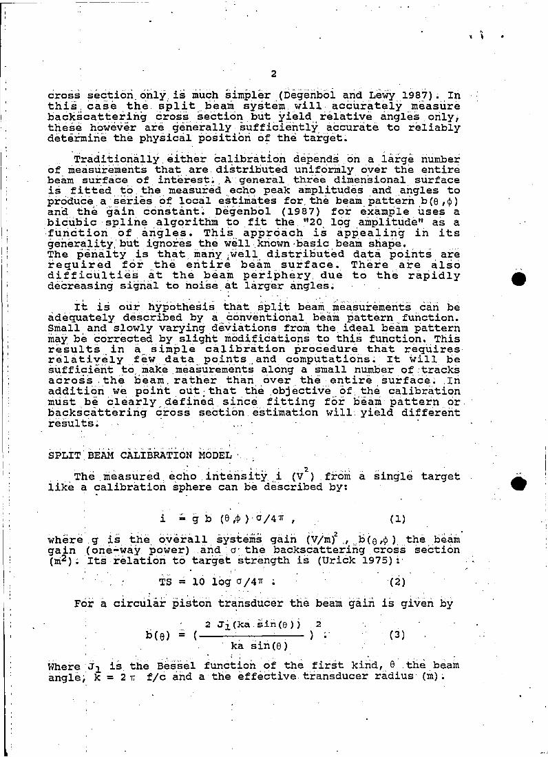
cross sectiori.onlY is milch simpler (Degenboi and Lewy 198'7). In '.thii, cas~ the. s~lit.b~a~ system will~c~~ratelymiascirebackscattering cross section but yield relative anglas orily,these however are generally sufficiently ac~urate to reliablydeterminä the physical position 6~ the target.
Trad~t~onallye~ther cal~brat~on depends on a large numberof measurements that are distributed uniformly over the entirebeam ·surface. of .. interest. A ' general. three dimensional surfaceis fitted to themeasured echo peak amplitudes and angles toproduce. a' series cf local estimates for., the beam pattern b(e,<1»and the gain 6onstant; Degenbol (1987) for example ~ses a.bic~bic .spline .algorithm to fit the, "20 log amplitude" as a,function of arigles. Tbis ap~roach i~ appealing in itsgeneralitYe' but ignores the well· krioWn -basic beam sbape. . .The p,enalty is th.~t, ~al,lYtwell,~istributed da:tä points, al:"erequ~red forthe ent~re beam surface. There are alsodifficulties ät the beain periphery due to the rapidlydecreasing signal to rioise.~t larger angles.
I ; , ,,'" ~., ': " ,~ ,. • • ~ _. , 1 • ',~
It is our hypotbesis that split beam measuremerits can beadeqUately deseribed by a conventional beam pattern. function.Small and slowly varying deviations from the ideal beam patternmay be correeted by sligbt modific:ations to this function. Thisresults in asimple calibrcition ~roc:edure that reqtiiresrelatively few data points and computatiöns~' It will besufficientto make.measurements along a small number of·tracksaeroBs .the ~eam. rather thein over the'entire surface: Inaddition ..we point out· that tbe "objective., of,.the calibrationmustbi clearly definid.since fitting fbr beam pattern erbackscattering cross section estimation will,yield differentresults~ .
'"
SPLITBEAM CALIBRATION MODEL-0( ~' , ,~ : ~; 2. P.
The.measured.echo ~ntens~ty ~ (V) from a single targetlike a calibration sphere can be described by:
•
i = g b (e,<1»' a /4 1T , (1)
where 9 is thä. overall systems gain. (v/m)2 , b (e;9). the beamgain (one-way power) and a- the backscatteringcross section(m2 ): Its relation to target strength is (Urick 1975):'
(2)
For a c!rcuiar piston transducer tbe beam gain is given by
- (--...;...-.-.--;..--ka sin(e)
b(e)2 Ji(ka.sin(8» . 2
) : . (3)
where ,Jl is thä Bessel functlon cf the first kirid, e'.tbe beamangle, k = 2 TI f/c and a the effective transducer radius (m) •
(4) .
(6)<-•
3
,For convenience and computational ease we have used an
approximate beamgaih'function which is given by approximatinqthe second .order expansion of the square root of b(8) by anexponential.fuhction (Appendix 1)~
. ka 2. b (e ). - exp - (-:-- s in (8) ) •
2
Our ec60 sou~de~ ieasures t6e fore/aft angle a andstarboard/port· angle ß (Figure 1)~ The transformation tospherical coordinates 8 and </l is given by:
tan(8) = ( tan2 (a) + ta~2 (ß) ) ~ (5)
tan(ß) .tan(8) - --
tan(a)
. ~q~ivalent expresiions for 8 ar~ so~e ti~es ,used (e.g.Degenbol 1987, Foote et;al. 1986). When polar .coordinates areemployed to.describe .the angles that are measured by the splitbeam echo sounder (Bodholt.1986, Ehrenberg 1981) thentheconversion equations use sin 8, sina and sinß; .,
~qciations(i) a~d. (4) yiel~s ~'si~~ie expression toestimate the beam gain b(8):
(7)
.Where v and 8 are the measured peak amplit~de and offaxisangle arid a is the known backscattering cross'section for thecalibration sphere~ The parameters .gi, kal and 81 are estimatedbyleast· squares non linear r~gref3sion•.The offset .ar:gle. 81 isrequired to produce a good f~t and represents an~d~osyncracy
of the echo sounder we used. Note that .the model so far isindependent of'</l;' . .
Normally. the estima.ted gain and beampattern are used' toproduce a calibratiori curve or equation for the. echo sounder iin order to convert measured amplitcides andangles fram unknowntargetsto.backscatt~ringciross section e~timates. Wedo riotrecommend. this procedure as it optimizes the beam pattern fit'and not the target strength cali~r~t~on. .
. .For optimal backscattering estimation
backscattercalibration model: .
4n- v 2
.,~ ,-
we.use the
(8)
4• _,.,1
METHODS
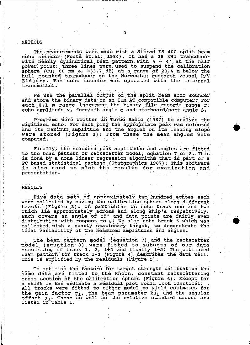
The. ineasurements were. made ..with ,aSimrad ES 400 ~piit beamecho ,seunder' (Foote et.al. ·1984) ~ Ithas' a 38. kHz transducerwith 'nearly cylindrical beam pattern.\.lith. e - 4°., at ,the halfpower: point ~ Three lines ware used to suspend. the c~l1ibrationsphere (Cu,. 60 mm rtJ" -33.7dB) at a range of 20~4 m below thehull .. mounted . transduceren the Norilegian research vesseil R/VEldjarn. Theecho sounder was operated with the internaltransnlitter •
, We use the parallel output of, the split· beam echo sounderand'store the binary data' onian. IBM AT .. ,compatible cömputer~' Foreach '0 ~ 1 m range increment. the binari . file records range r,echo amplitude v, fore/aft ängle ci and' starboard/port angle ß.
'. .
. progranis ware written iri 'Turbö Basic, eÜ387)to arialyze thedigitized echo~ For each ping theappropriate peak was selectedand its maximum amplitude andthe angles on its leading slopewere~stored (Figure 2). : Fröni these the mean angles werecomputed. :, '.
,F~nally, themeasured peak amplitudes and,angles are,fittedto thebeam.pattern or backscatter model, eqilation 7 or.8 •. Thisis done by a none linearregressionalgorithm that'is,partof aPC based statistical package(Statgraphics 1987)~ This softwareis also ,used tö plotthe results for examination andpresentation. ':' "
.. ,RESPLTS
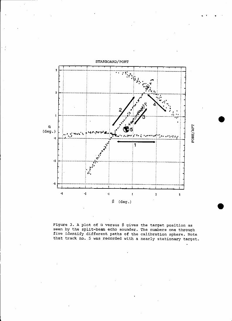
Five'data setsof approximately two' ,hundred echoes each.were collected by movingthe cialibration sphere alo'ng differenttracks', (Figure 3); In pärticular we note track 'one ~md twowhich lieapproxiniately 'across and along ship' s respectively.Each 'covers' an, angle ,of ±5 ° and data points .are. fairly , evendistribution:with respecit. to e; We also riote.track 5 which was "ciollected, with. a nearly stationary target,. to demonstrate thelocal:variability of ,the measured·amplitudes and angles.
: ..".. .The bea'ni'pattern modei.(equation 7) and' the .backscatter
model (equatiöri 8) ware' fi ttäd .to subsets of' our, dataconsistirig of. track 1; 2; 1-1:"2 arid finally 1-5;. The estiInatedbeam pattern'for track 1+2 .(Figure 4) describes the data .well.This is amplified by the residuals (Fiqure 5); "
Tc optimise the factörsfor ta.rget strerigth'cal!bratiori'thesame dat~ ,are fittedto the kri6wn,constant ba6ksc~ttering
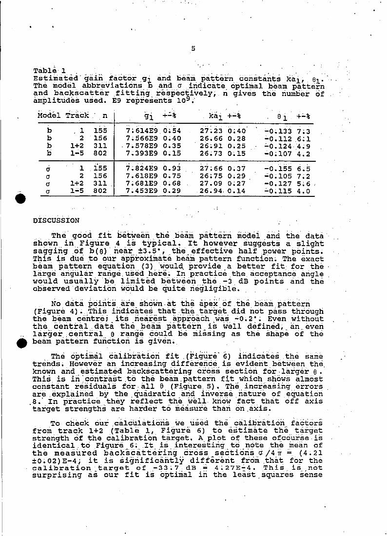
cross,section of the calibration sphere (Figure 6). Except fora shift in the ordinate a residual plot woüld look identical~ .All tracks were fitted to either model to yield estimates forthe gairi factor gi, .the beam parame~er kal a.nd the.angularoffset ei; These as well as the relat~ve standard errors arelisted in Table 1. .
The' good fit between tlie beam pattern modei and the datasliowriin, Figure 4 is typical. It hciwever suggests a slightsagging cif b(s)' near ±3.5°, ,the effective half power points;This is dueto our approximate beam pattern function; ,The exactbeam pattern equation (3) ·would. provide ,a better fit, for the .1arge angular range used here; In practicethe acceptance angle ,would usua11ybe limited bet~~eri the -3dB points and theobserved deviation wö~ld be quite riegligible. , ,,' ,
No data points are ,shovin,at i:he apex:of the beam pattern(Figure 4); ,Tliis indicates thatthe,target did not pass througlitlie beamcentre; its nearest approach was -0.2°., Even withoutthe central ,data the, beäIii pattern is ~Eül defined, an" even1arger ;centrä~e range cou1d be missing as the shape of thebeam pattern functiori is given.
The opt~ma1 ca1~brat~on f~t (F~gure 6) ~nd~cates, the sametrends. However an increasing difference is evident between theknown and, estimated backscattering cross sectiöri for .1arger e ..This, is in'coritrast,tö the beam,pattern fit which shöws almostconstant residua1s for. all e (Figure, 5). The" increasing errorsare exp1ained by the"quädratic arid inverse nature of equation
.8.' In practice" they ref1ectthe ~e11, know fact that offaxistarget strengths are harder tö measure tliari ori.axis.
,To check ourc'a1cu1atiön~.,we .used the'.C?ä~i~ratioii.. factorsfrom track 1+2 (Table 1, F~gure 6) tO,est~mate the,targetstrerigth cf the ca1ibration target. A plot of theseofcourse,isidentica1 . to Figure 6;,It is iriterestirig tö notethe mean ofthe nieasured backscattering cross, sectiöris, 0: /4';' = (4.21±0;02)E-4j it is significärit1y different fram ,that for theca~ibration.target of -33; 7.. dB :;: 4 ;27E::4. ,This iS.,.n6tsurprising as our fit isoptimal in the, least. squares sense
I
.,:
I ,~ ":I 6I
!
wliiie·,the average i5 a line~roperatiori~ The d1fference betweenthe two values .. is 0 ~ 06 dB and will diminish whem, the acceptedechoes.are limitedby thel~3 dB points. The difference will'totally disappear. when a' linear' distanci"e measure rather . than',distance square is used for·fitti~g•
. The relative standard e~~orsgivenin Table 1 indicatethehigh precisiori.of ourparameter estimates~ The largest error. onthe e;ghtgl es,timates is, .0,nlY 0 .~% (0.94 dB)and those .,for k~lare even smalle;-. Errors ,.l.n :6.i .<1.0 not· exc~ed.7~ .(0.3 ~B), .thl.srelatively large value indicates,that our 'functl.ons are quiteinsensitive to this parameter., .
For each niodei' several' target tracks .ware .. arialysed,omitt~ng tra~k 1~5 the .v.ar~ati?~.betwe~ngl'es~imates ~s of theorder of 0.05 dB. Thl.s l.S sl.ml.lar to ·the',dl.ffe:J:;"ence'betweenmodels for this parameter estimate based on .,track 1+2. Offaxisthe differerice in models will: be more significant; :
Nea~ ~he acoustica~is iri estimated ~ac~sca~tering crosssectiC?n w.ill, be donii,nated ,by, the error~ in gl and ,.a"2~, We, f~elthat gl l.S reproducl.ble to, 0.05 dB when a few hundred echoesare used; Observations of.the almost stationarytarget (Figura3, track 5) provide an estimatefor the rela~ive standarddeviation foreäch measured' a 2 of. l~ 5% (O~ 06 dB). A largervalue is exPected' fo~ offaxis arid smaller echoes; , .
. \
Tc illustrate the efiective difference b~t~eeri theestiriüited parameters (Table: 1) 'we have plotted the iiormalizedcalibration faetor, , (Figure 7). It is,. b"clsed on ,equätion, (8) anduses the backscatter calibration from track 1+2 as.a reference.As expected thedata. from track 1 and 2 lie on eithe~ side of'thestraight line thät represeiits ,track J.+2~, For, 'sniäll e a .maximum differenceof 2% is obserVed while off axis much. largerdevia~iöns oceur; This ,suggests ,that the bearii pattern eqÜationsfor track 1 and, 2 ',are indeed slightly different. wä also' showthe beampatterncalibratiori from trackl+2,. e"eiri'at the ~3 dBpoints i t deviates . strongly fromthe strait'line ~ Thesedeviatioris are impo~tänt when targets outside the half powerpoints must be measured. '. .
. . . .1 ' '. ' '.. •
our data points are riearly ideally distributed for the beampatterri fit (Figure 4); For the backscattEir"fit we howeverwould like to havean increasing nÜroberofpoints, (proportionalto e)·. as ' e increases 'toreflect the' lärger freqÜericy, of fishtargets in:the, beam periphery: "In addition i~ älso. 1s desirablet6 have at least three or more tracks that cross the beamsystematically, not just two as inthis particular ciase~ Workon more complete data set~ i5, ,in progress ~ ','. ". ,...
, We ,have" obseryed an ..ang~J.a~, c?ff:,~et,.,ei."'7 .-o~J.·,. '7his is ~fthe same magnitude but not equl.valent tothe offset l.n a and ßfound'by Bodho~t (1986) for ~~ ideri~ical 'split beam'system~
. '.. .
we have deliberately chosenasiInple beam pattern' andcalibratiori model' and ·'found it adequate. to 'describe 6ur datä~
.;;" .•
..
•
, '., 7
However several improvements are possible and may be desirablewhen more measurements are available: .
1. Exact beam pattern model; e.g. circular piston orrectangular.
2. Include a small e dependencete correct for rotational,asymmetries. A small ~ dependence is suggested by our dataand those presented by Reynisson (1987a).
3. Use the angles a and ß rather than e and ~. This issuggested by the above-mentioned angular offset(Bodholt 1986). . ,
The calibration method presented here is·ofcourseapplicable to adual beam system. However it also could be usedfor the calibration of a single beam transducer or echo sounderwhen the anglesa and ß have oeen measured geometrically, as is .'usually the case when a calibration facility is used. Fitting abeam pattern er target strength calibration model to a range ofobservations will certainly provide a better calibration than asingle on-axis measurement. "
We have realized fr~m'calibration exercises and fish datathat a beam threshold must be applied in order to maintain thesignal-to-noise ratio:and stability in theangle determinationparticularly for small echoes. Inpractice we thereforeconcentrate on obtaining the correct' beam gain matrix within
. the -3 dB points, rather than to stretch the observation volume ,andcalibrati6n procedures to lirger angles where poor ...backscattering cross section estimates arid severe thresholdbiasing are inevitable.
ACKNOWLEDGEMENT
•..
One of us (R.K.) is grateful for the,hospitality andstimulating working. conditions "which, he· enjoyed during aProfessional Development at the Institute ,of Marine Research,Bergen. A ,germane discussion with P. Degenbol~is gladlyacknowledged.
8
REFERENCES, ,
Bodholt H. 1986.Angle measurements with simrad'ES'38 split oeamtränsducer.Simrad Report No. '345 86~·11~,27., p12.
Degenbol P., P. LewY. 1987.'Interpretation of target' strength information from split beamdata. International' symposium on Fisheries Acoustics, June22-26, 1987, Seatt1e, washi~gton, USA. p13.
Ehrenberg J. E. 1981. ~ " ,Analysis of split beam backscattering cross section'estimatioriand ~ing1e echo iso1ati~ntechniques. A~p1ied pbisicsLaboratory, 'University' of· Washirigton~' Report No. APL~UW 8108,May 1981, p24. '
Foote K.G., A. Agleri,' 0;' Nakken'. 1986.Measurement of fish target strengtli with a split beam echosounder. J. AcouSt. 'Soc. Am.!'80:612-621. " "
"
Foote K.G. i H.P. Knudsen, G. vestnes, R. Brede, R;L Nie1sen.1981.Improved calibration of hydroacoustic eqUipment with copperspheres. ICES, C.M. 1981.B:20.
~o6teK.G;,'~.H. ~~istenseri, H.'Solli. 1~84~ .'Trül1s of a new s~l~t~bea~"~c~o sounder. ICES, .'~;M. 1984/B:21.
Reynisson P. 1987a:, 'Measurements of 'the Beam Pattern arid compensation Errors' ofSplit~Beam Echo Sounders. International Symposium on FisheriesAcoustics, June 22-26, 1987, Seattle, washington"USA. p16.
, .Reynisson P. 1987b.,. . . .A Geometrie Method for Measuring the Equivalent Beam Angles ofHull Mounted Transducers. International Symposium on FisheriesAcoustics, June 22-26, 1987,Seattle, Washington, USA. ~14.
statgraphics 1987.Version 2; 6, STSC PLUS*WARE.:,
Turbo-Basic 1987.Borland International Inc;
- ,Urick,R.J. 1975. .princip1es of underwater sound. MCGraW-Hi11, New York, USA.
•
•
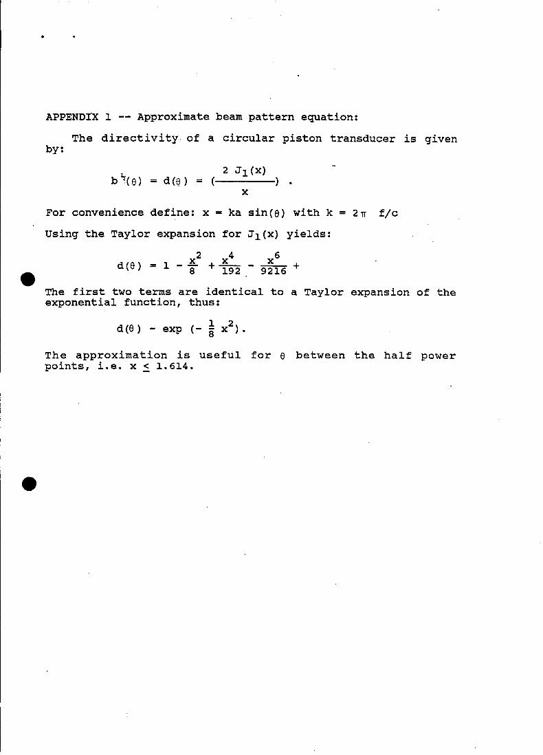
APPENDIX 1 -- Approximate beam pattern equation:
The directivity of a circular piston transducer is givenby:
2 J1 (x)b ~(6) = d (~) = ( ) •
x
For convenience define: x = ka sin(8) with k = 2~ f/c
Using the Taylor expansion for J1(x) yields:
x 2 x 4 x 6d (6) = 1 -"8 + 192 - 9216 +
The first two terms are identical to a Taylor expansion of theexponential function, thus:
1 2dca) - exp (- 8 x ).
The approximation is useful for e between the half powerpoints, i.e. x ~ 1.614.
DOWNZ
•
XFORE
II
II
II
.... .... ....." ....
y
STARBOARD
•
•Figure 1. Used coordinate·system. The fore/aft angle a andstarboard/port angle ß are measured in the x/z and Y/Z planerespectively. Spherical coordinates e and ~ are also shown.
•Figure 2. Single pulse from the sphere at 20.4 m depth. Onlydata above the noise threshold are collected. Small dotsindicate actual data'points, with angle data available onthe rising part of the pulse. A single-target peak must exeedthe peak threshold, and is characterized by the peak amplitude,width at half amplitude, W, angles a and ß and their standarddeviation.
Figure 3. A plot of a versus ß gives the target position asseen by the split-beam echo sounder. The numbers one throughfive identify different paths of the calibration sphere. Notethat track no •.5 was recorded with a nearly stationary target.
··i·····..·..··················..····~··········,~·i··· ..·..·········i··························..·····f·································f······················..·······"i"~ i· }:..; i : i