CHAPTER 5

TOPOLOGY AND GEOMETRY OF SURFACES

Compact (and some noncompact) surfaces are a favorite showcase for variousbranches of topology and geometry. They are two-dimensional topological mani-folds, which can be supplied with a variety of naturally defined differentiable andRiemannian structures. Their complete topological classification, which coincideswith their smooth (differentiable) classification, is obtained via certain simple in-variants. These invariants allow a variety of interpretations: combinatorial, analyt-ical and geometrical.

Surfaces are also one-dimensional complex manifolds; but, surprisingly, thecomplex stuctures are not all equivalent (except for the case of the sphere), althoughthey can be classified. This classification if the first result in a rather deep area atthe junction of analysis, geometry, and algebraic geometry known as Teichmullertheory, which recently has led to spectacular applications in theoretical physics.

In this chapter we study the classification of compact surfaces (two-dimen-sional manifolds) from various points of view. We start with a fundamental prepara-tory result, which we will prove by using a beautiful argument based on combina-torial considerations.

5.1. Two big separation theorems: Jordan and Schoenflies

The goal of this section is to prove the famous Jordan Curve Theorem, whichwe will need in the next section, and which is constantly used in many areas ofanalysis and topology. Note that although the statement of the theorem seemsabsolutely obvious, it does not have a simple proof.

5.1.1. Statement of the theorem and strategy of proof. Here we state thetheorem and outline the main steps of the proof.

DEFINITION 5.1.1. A simple closed curve on a manifold M (in particular onthe plane R2) is the homeomorphic image of the circle S1 in M , or equivalentlythe image of S1 under a topological embedding S1 ! M .

THEOREM 5.1.2 (Jordan Curve Theorem). A simple closed curve C on theplane R2 separates the plane into two connected components.

COROLLARY 5.1.3. A simple closed curve C on the sphere S2 separates thesphere into two connected components.

125

126 5. TOPOLOGY AND GEOMETRY OF SURFACES

PROOF. The proof is carried out by a simple but clever reduction of the JordanCurve Theorem to the nonplanarity of the graphK3,3, established in ??

Suppose that C is an arbitrary (not necessarily polygonal) simple closed curvein the plane R2. Suppose l and m are parallel support lines of C and p is a lineperpendicular to them and not intersecting the curve. Let A1 and A2 be points ofthe intersections of C with l andm, respectively. Further, letB3 be the intersectionpoint of l and p. The pointsA1 andA2 divide the curveC into two arcs, the “upper”one and the “lower” one. Take a line q in between l and m parallel to them. Bycompactness, there is a lowest intersection point B1 of q with the upper arc and ahighest intersection point B2 of q with the lower arc. Let A3 be an inner point ofthe segment [B1, B2] (see the figure).

q pz0

m ln

w b

FIGURE 5.1.1. Proof of the Jordan Curve Theorem

We claim that R2 \ C is not path connected, in fact there is no path joiningA3 and B3. Indeed, if such a path existed, by Lemma ?? there would be an arcjoining these two points. Then we would have nine pairwise nonintersecting arcsjoining each of the points A1, A2, A3 with all three of the points B1, B2, B3. Thismeans that we have obtained an embedding of the graph K3,3 in the plane, whichis impossible by Theorem 5.2.4. !

5.1.2. Schoenflies Theorem. The Schoenflies Theorem is an addition to theJordan curve theorem asserting that the curve actually bounds a disk. We state thistheorem here without proof.

THEOREM 5.1.4 (Schoenflies Theorem). A simple closed curveC on the planeR2 separates the plane into two connected components; the component with boundedclosure is homeomorphic to the disk, that is,

R2 ! C = D1 "D2, where D1 #D2 = " and D1 $ D2.

COROLLARY 5.1.5. A simple closed curve C on the sphere S2 separates thesphere into two connected components, each of which has closure homeomorphicto the disk, that is,

S2 ! C = D1 "D2, where D1 #D2 = " and Di $ D2, i = 1, 2.

5.2. PLANAR AND NON-PLANAR GRAPHS 127

C

L1

L2

FIGURE 5.2.1. The polygonal lines L1 and L2 must intersect

5.2. Planar and non-planar graphs

5.2.1. Non-planarity ofK3,3. We first show that the graphK3,3 has no polyg-onal embedding into the plane, and then show that it has no topological embeddingin the plane.

PROPOSITION 5.2.1. [The Jordan curve theorem for broken lines] Any bro-ken line C in the plane without self-intersections splits the plane into two pathconnected components and is the boundary of each of them.

PROOF. Let D be a small disk which C intersects along a line segment, andthus dividesD into two (path) connected components. Let p be any point inR2\C.From p we can move along a polygonal line as close as we like to C and then,staying close to C, move inside D. We will then be in one of the two componentsof D \ C, which shows that R2 \ C has no more than two components.

It remains to show that R2 \C is not path connected. Let ! be a ray originatingat the point p % R2 \ C. The ray intersects C in a finite number of segments andisolated points. To each such point (or segment) assign the number 1 if C crosses !there and 0 if it stays on the same side. Consider the parity "(p) of the sum S of allthe assigned numbers: it changes continuously as ! rotates and, being an integer,"(p) is constant. Clearly, "(p) does not change inside a connected component ofR2 \C. But if we take a segment intersecting C at a non-zero angle, then the parity" at its end points differs. This contradiction proves the proposition. !

We will call a closed broken line without self-intersections a simple polygonalline.

COROLLARY 5.2.2. If two broken lines L1 and L2 without self-intersectionslie in the same component of R2 \ C, where C is a simple closed polygonal line,with their endpoints on C in alternating order, then L1 and L2 intersect.

PROOF. The endpoints a and c of L1 divide the polygonal curve C into twopolygonal arcs C1 and C2. The curve C and the line L1 divide the plane into threepath connected domains: one bounded by C, the other two bounded by the closed

128 5. TOPOLOGY AND GEOMETRY OF SURFACES

curves Ci " L, i = 1, 2 (this follows from Proposition 5.2.1). Choose points b andd on L2 close to its endpoints. Then b and d must lie in different domains boundedby L1 and C and any path joining them and not intersecting C, in particular L2,must intersect L1. !

PROPOSITION 5.2.3. The graph K3,3 cannot be polygonally embedded in theplane.

PROOF. Let us number the vertices x1, . . . , x6 ofK3,3 so that its edges consti-tute a closed curve C := x1x2x3x4x5x6, the other edges being

E1 := x1x4, E2 := x2x5, E3 := x3x6.

Then, ifK3,3 lies in the plane, it follows from Proposition 5.2.1 that C divides theplane into two components. One of the two components must contain at least twoof the edges E1, E2, E3, which then have to intersect (by Corollary 5.2.2). This isa contradiction which proves the proposition. !

THEOREM 5.2.4. The graph K3,3 is nonplanar, i.e., there is no topologicalembedding h : K3,3 #! R2.

The theorem is an immediate consequence of the nonexistence of aPL-embeddingofK3,3 (Proposition 5.2.3) and the following lemma.

LEMMA 5.2.5. If a graphG is planar, then there exists a polygonal embeddingof G into the plane.

PROOF. Given a graphG & R2, we first modify it in small disk neighborhoodsof the vertices so that the intersection of (the modified graph) G with each disk isthe union of a finite number of radii of this disk. Then, for each edge, we coverits complement to the vertex disks by disks disjoint from the other edges, choose afinite subcovering (by compactness) and, using the chosen disks, replace the edgeby a polygonal line. !

5.2.2. Euler characteristic and Euler theorem. The Euler characteristic ofa graph G without loops embedded in the plane is defined as

$(G) := V ' E + F,

where V is the number of vertices andE is the number of edges ofG, while F is thenumber of connected components ofR2\G (including the unbounded component).

THEOREM 5.2.6. [Euler Theorem] For any connected graph G without loopsembedded in the plane, $(G) = 2.

5.3. SURFACES AND THEIR TRIANGULATIONS 129

PROOF. At the moment we are only able to prove this theorem for polygonalgraphs. For the general case we will need Jordan curve Theorem Theorem 5.1.2.The proof will be by induction on the number of edges. For the graph with zeroedges, we have V = 1, E = 0, F = 1, and the formula holds. Suppose it holds forall graphs with n edges; then it is valid for any connected subgraphH of G with nedges; take an edge e from G which is not inH but incident toH , and add it toH .Two cases are possible.

Case 1. Only one endpoint of e belongs toH . Then F is the same for G as forH and both V and E increase by one.

Case 2. Both endpoints of e belong to toH . Then e lies inside a face ofH anddivides it into two.1 Thus by adding e we increase both E and F by one and leaveV unchanged. Hence the Euler characteristic does not change. !

5.2.3. Kuratowski Theorem. We conclude this subsection with a beautiful the- small print for parts outside ofthe main line: no proofs or too

difficultorem, which gives a simple geometrical obstruction to the planarity of graphs. We do notpresent the proof (which is not easy), because this theorem, unlike the previous one, is notused in the sequel.

THEOREM 5.2.7. [Kuratowski] A graph is nonplanar if and only if it contains, as atopological subspace, the graph K3,3 or the graph K5.

REMARK 5.2.8. The words “as a topological subspace” are essential in this theorem.They cannot be replaced by “as a subgraph”: if we subdivide an edge of K5 by adding avertex at its midpoint, then we obtain a nonplanar graph that does not contain either K3,3

orK5.

EXERCISE 5.2.1. Can the graphK3,3 be embedded in (a) the Mobius strip, (b)the torus?

EXERCISE 5.2.2. Is there a graph that cannot be embedded into the torus?

EXERCISE 5.2.3. Is there a graph that cannot be embedded into the Mobiusstrip?

5.3. Surfaces and their triangulations

In this section, we define (two-dimensional) surfaces, which are topologicalspaces that locally look like R2 (and so are supplied with local systems of coor-dinates). It can be shown that surfaces can always be triangulated (supplied witha PL-structure) and smoothed (supplied with a smooth manifold structure). We proof will be added here or later

an easy consequence of PLwill not prove these two assertions here and limit ourselves to the study of trian-gulated surfaces (also known as two-dimensional PL-manifolds). The main resultis a neat classification theorem, proved by means of some simple piecewise lineartechniques and with the help of the Euler characteristic.

1It is here that we need the conclusion of Jordan curve Theorem Theorem 5.1.2 in the case ofgeneral graphs. The rest of the argument remains the same as for polygonal graphs.

130 5. TOPOLOGY AND GEOMETRY OF SURFACES

5.3.1. Definitions and examples.

DEFINITION 5.3.1. A closed surface is a compact connected 2-manifold (with-out boundary), i.e., a compact connected space each point of which has a neigh-borhood homeomorphic to the open 2-disk Int D2. In the above definition, con-nectedness can be replaced by path connectedness without loss of generality (see??)

A surface with boundary is a compact space each point of which has a neigh-borhood homeomorphic to the open 2-disk Int D2 or to the open half disk

Int D21/2 = {(x, y) % R2|x " 0, x2 + y2 < 1}.

EXAMPLE 5.3.2. Familiar surfaces are the 2-sphere S2, the projective planeRP 2, and the torus T2 = S1 ( S1, while the disk D2, the annulus, and the Mobiusband are examples of surfaces with boundary.

S2 T 2 D2

FIGURE 5.3.1. Examples of surfaces

DEFINITION 5.3.3. The connected sum M1#M2 of two surfaces M1 and M2

is obtained by making two small holes (i.e., removing small open disks) in thesurfaces and gluing them along the boundaries of the holes

EXAMPLE 5.3.4. The connected sum of two projective planes RP 2#RP 2 isthe famous Klein bottle, which can also be obtained by gluing two Mobius bandsalong their boundaries (see Fig.??). The connected sum of three tori T2#T2#T2

is (topologically) the surface of a pretzel (see Fig.??).

FIGURE 5.3.2. Klein bottle and pretzel

5.3. SURFACES AND THEIR TRIANGULATIONS 131

5.3.2. Polyhedra and triangulations. Our present goal is to introduce a com-binatorial structure (called PL-structure) on surfaces. First we we give the corre-sponding definitions related to PL-structures.

A (finite) 2-polyhedron is a topological space represented as the (finite) unionof triangles (its faces or 2-simplices) so that the intersection of two triangles iseither empty, or a common side, or a common vertex. The sides of the trianglesare called edges or 1-simplices, the vertices of the triangles are called vertices or0-simplices of the 2-polyhedron.

Let P be a 2-polyhedron and v % P be a vertex. The (closed) star of v in P(notation Star(v, P )) is the set of all triangles with vertex v. The link of v in P(notation Link(v, P )) is the set of sides opposite to v in the triangles containing v.

A finite 2-polyhedron is said to be a closed PL-surface (or a closed triangu-lated surface) if the star of any vertex v is homeomorphic to the closed 2-disk withv at the center (or, which is the same, if the links of all its vertices are homeomor-phic to the circle).

Stx Lk y

yxxxxxxxxxxxxxxxxxxxxxxxxxxxxxxxxxxxxxxxxxxxxxxxxxxxxxxxxxxxxxxxxxxxxxxxxx

FIGURE 5.3.3. Star and link of a point on a surface

A finite 2-polyhedron is said to be a PL-surface with boundary if the star ofany vertex v is homeomorphic either to the closed 2-disk with v at the center or tothe closed disk with v on the boundary (or, which is the same, if the links of all itsvertices are homeomorphic either to the circle or to the line segment). It is easy tosee that in a PL-surface with boundary the points whose links are segments (theyare called boundary points) constitute a finite number of circles (called boundarycircles). It is also easy to see that each edge of a closed PL-surface (and eachnonboundary edge of a surface with boundary) is contained in exactly two faces.

A PL-surface (closed or with boundary) is called connected if any two verticescan be joined by a sequence of edges (each edge has a common vertex with theprevious one). Further, unless otherwise stated, we consider only connected PL-surfaces.

A PL-surface (closed or with boundary) is called orientable if its faces can becoherently oriented; this means that each face can be oriented (i.e., a cyclic orderof its vertices chosen) so that each edge inherits opposite orientations from theorientations of the two faces containing this edge. An orientation of an orientablesurface is a choice of a coherent orientation of its faces; it is easy to see that thatany orientable (connected!) surface has exactly two orientations.

132 5. TOPOLOGY AND GEOMETRY OF SURFACES

A face subdivision is the replacement of a face (triangle) by three new facesobtained by joining the baricenter of the triangle with its vertices. An edge sub-division is the replacement of the two faces (triangles) containing an edge by fournew faces obtained by joining the midpoint of the edge with the two opposite ver-tices of the two triangles. A baricentric subdivision of a face is the replacementof a face (triangle) by six new faces obtained by constructing the three medians ofthe triangles. A baricentric subdivision of a surface is the result of the baricentricsubdivision of all its faces. Clearly, any baricentric subdivision can be obtainedby means of a finite number of edge and face subdivisions. A subdivision of aPL-surface is the result of a finite number of edge and face subdivisions.

Two PL-surfaces M1 and M2 are called isomorphic if there exists a homeo-morphism h : M1 ! M2 such that each face ofM1 is mapped onto a face ofM2.Two PL-surfaces M1 and M2 are called PL-homeomorphic if they have isomor-phic subdivisions.

FIGURE 5.3.4. Face, edge, and baricentric subdivisions

EXAMPLE 5.3.5. Consider any convex polyhedron P ; subdivide each of itsfaces into triangles by diagonals and project this radially to a sphere centered inany interior point of P . The result is a triangulation of the sphere.

If P is a tetrahedron the triangulation has four vertices. This is the minimalnumber of vertices in a triangulation of any surface. In fact, any triangulationof a surface with four vertices is equivalent of the triangulation obtained from atetrahedron and thus for any surface other than the sphere the minimal number ofvertices in a triangulation is greater then four.

EXERCISE 5.3.1. Prove that there exists a triangulation of the projective planewith any given number N > 4 of vertices.

EXERCISE 5.3.2. Prove that minimal number of vertices in a triangulation ofthe torus is six.

5.4. Euler characteristic and genus

In this section we introduce, in an elementary combinatorial way, one of thesimplest and most important homological invariants of a surface M – its Eulercharacteristic $(M). The Euler characteristic is an integer (actually defined for amuch wider class of objects than surfaces) which is topologically invariant (and,in fact, also homotopy invariant). Therefore, if we find that two surfaces havedifferent Euler characteristics, we can conclude that they are not homeomorphic.

5.4. EULER CHARACTERISTIC AND GENUS 133

5.4.1. Euler characteristic of polyhedra.

DEFINITION 5.4.1. The Euler characteristic $(M) of a two-dimensional poly-hedron, in particular of a PL-surface, is defined by

$(M) := V ' E + F ,

where V,E, and F are the numbers of vertices, edges, and faces ofM , respectively.

PROPOSITION 5.4.2. The Euler characteristic of a surface does not depend onits triangulation. PL-homeomorphic PL-surfaces have the same Euler character-istic.

PROOF. It follows from the definitions that we must only prove that the Eulercharacteristic does not change under subdivision, i.e., under face and edge subdi-vision. But these two facts are proved by a straightforward verification. !

EXERCISE 5.4.1. Compute the Euler characteristic of the 2-sphere, the 2-disk,the projective plane and the 2-torus.

EXERCISE 5.4.2. Prove that $(M#N) = $(M) + $(N) ' 2 for any PL-surfaces M and N . Use this fact to show that adding one handle to an orientedsurface decreases its Euler characteristic by 2.

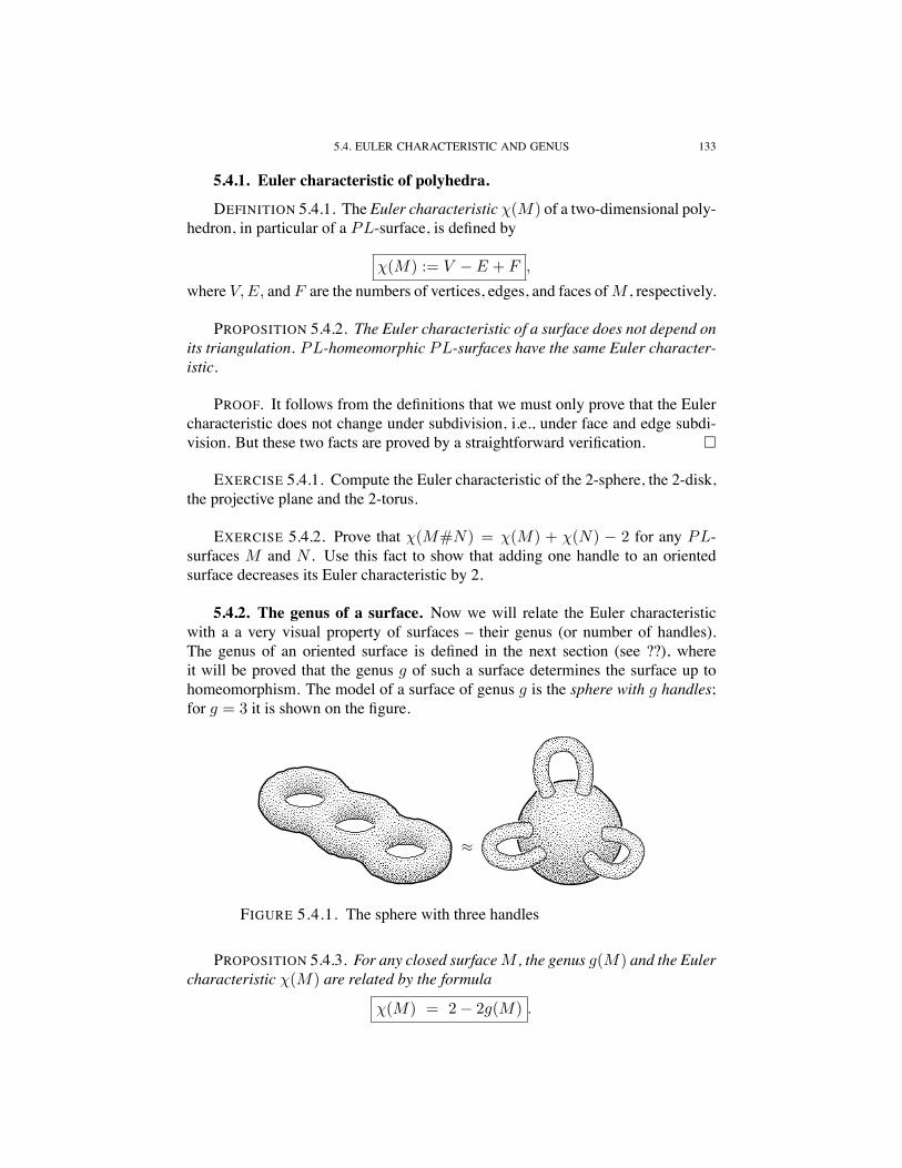
5.4.2. The genus of a surface. Now we will relate the Euler characteristicwith a a very visual property of surfaces – their genus (or number of handles).The genus of an oriented surface is defined in the next section (see ??), whereit will be proved that the genus g of such a surface determines the surface up tohomeomorphism. The model of a surface of genus g is the sphere with g handles;for g = 3 it is shown on the figure.

$

FIGURE 5.4.1. The sphere with three handles

PROPOSITION 5.4.3. For any closed surfaceM , the genus g(M) and the Eulercharacteristic $(M) are related by the formula

$(M) = 2' 2g(M) .

134 5. TOPOLOGY AND GEOMETRY OF SURFACES

PROOF. Let us prove the proposition by induction on g. For g = 0 (the sphere),we have $(S2) = 2 by Exercise ??. It remains to show that adding one handledecreases the Euler characteristic by 2. But this follows from Exercise ?? !

REMARK 5.4.4. In fact $ = %2 ' %1 + %0, where the %i are the Betti numbers(defined in ??). For the surface of genus g, we have %0 = %2 = 1 and %1 = 2g, sowe do get $ = 2' 2g.

5.5. Classification of surfaces

In this section, we present the topological classification (which coincides withthe combinatorial and smooth ones) of surfaces: closed orientable, closed nonori-entable, and surfaces with boundary.

5.5.1. Orientable surfaces. The main result of this subsection is the follow-ing theorem.

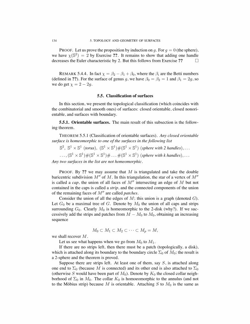
THEOREM 5.5.1 (Classification of orientable surfaces). Any closed orientablesurface is homeomorphic to one of the surfaces in the following list

S2, S1 ( S1 (torus), (S1 ( S1)#(S1 ( S1) (sphere with 2 handles), . . .. . . , (S1 ( S1)#(S1 ( S1)# . . .#(S1 ( S1) (sphere with k handles), . . .

Any two surfaces in the list are not homeomorphic.

PROOF. By ?? we may assume that M is triangulated and take the doublebaricentric subdivision M !! of M . In this triangulation, the star of a vertex of M !!

is called a cap, the union of all faces of M !! intersecting an edge of M but notcontained in the caps is called a strip, and the connected components of the unionof the remaining faces ofM !! are called patches.

Consider the union of all the edges of M ; this union is a graph (denoted G).Let G0 be a maximal tree of G. Denote by M0 the union of all caps and stripssurrounding G0. Clearly M0 is homeomorphic to the 2-disk (why?). If we suc-cessively add the strips and patches fromM 'M0 toM0, obtaining an increasingsequence

M0 & M1 & M2 & · · · & Mp = M,

we shall recoverM .Let us see what happens when we go fromM0 toM1.If there are no strips left, then there must be a patch (topologically, a disk),

which is attached along its boundary to the boundary circle !0 ofM0; the result isa 2-sphere and the theorem is proved.

Suppose there are strips left. At least one of them, say S, is attached alongone end to !0 (because M is connected) and its other end is also attached to !0

(otherwise S would have been part ofM0). Denote byK0 the closed collar neigh-borhood of !0 in M0. The collar K0 is homoeomorphic to the annulus (and notto the Mobius strip) because M is orientable. Attaching S to M0 is the same as

5.5. CLASSIFICATION OF SURFACES 135

PATCH

CAP

CAP

CAP

STRIP

STR

IP

STRIP

PATCH

CAP

CAP

CAP

STRIP

STR

IP

STRIP

PATCH

CAP

CAP

CAP

STRIP

STR

IP

STRIP

PATCH

CAP

CAP

CAP

STRIP

STR

IP

STRIP

PATCH

CAP

CAP

CAP

STRIP

STR

IP

STRIP

PATCH

CAP

CAP

CAP

STRIP

STR

IP

STRIP

PATCH

CAP

CAP

CAP

STRIP

STR

IP

STRIP

PATCH

CAP

CAP

CAP

STRIP

STR

IP

STRIP

PATCH

CAP

CAP

CAP

STRIP

STR

IP

STRIP

PATCH

CAP

CAP

CAP

STRIP

STR

IP

STRIP

PATCH

CAP

CAP

CAP

STRIP

STR

IP

STRIP

PATCH

CAP

CAP

CAP

STRIP

STR

IP

STRIP

PATCH

CAP

CAP

CAP

STRIP

STR

IP

STRIP

PATCH

CAP

CAP

CAP

STRIP

STR

IP

STRIP

PATCH

CAP

CAP

CAP

STRIP

STR

IP

STRIP

PATCH

CAP

CAP

CAP

STRIP

STR

IP

STRIP

PATCH

CAP

CAP

CAP

STRIP

STR

IP

STRIP

PATCH

CAP

CAP

CAP

STRIP

STR

IP

STRIP

PATCH

CAP

CAP

CAP

STRIP

STR

IP

STRIP

PATCH

CAP

CAP

CAP

STRIP

STR

IP

STRIP

PATCH

CAP

CAP

CAP

STRIP

STR

IP

STRIP

PATCH

CAP

CAP

CAP

STRIP

STR

IP

STRIP

PATCH

CAP

CAP

CAP

STRIP

STR

IP

STRIP

PATCH

CAP

CAP

CAP

STRIP

STR

IP

STRIP

PATCH

CAP

CAP

CAP

STRIP

STR

IP

STRIP

PATCH

CAP

CAP

CAP

STRIP

STR

IP

STRIP

PATCH

CAP

CAP

CAP

STRIP

STR

IP

STRIP

PATCH

CAP

CAP

CAP

STRIP

STR

IP

STRIP

PATCH

CAP

CAP

CAP

STRIP

STR

IP

STRIP

PATCH

CAP

CAP

CAP

STRIP

STR

IP

STRIP

PATCH

CAP

CAP

CAP

STRIP

STR

IP

STRIP

PATCH

CAP

CAP

CAP

STRIP

STR

IP

STRIP

PATCH

CAP

CAP

CAP

STRIP

STR

IP

STRIP

PATCH

CAP

CAP

CAP

STRIP

STR

IP

STRIP

PATCH

CAP

CAP

CAP

STRIP

STR

IP

STRIP

PATCH

CAP

CAP

CAP

STRIP

STR

IP

STRIP

PATCH

CAP

CAP

CAP

STRIP

STR

IP

STRIP

PATCH

CAP

CAP

CAP

STRIP

STR

IP

STRIP

PATCH

CAP

CAP

CAP

STRIP

STR

IP

STRIP

PATCH

CAP

CAP

CAP

STRIP

STR

IP

STRIP

PATCH

CAP

CAP

CAP

STRIP

STR

IP

STRIP

PATCH

CAP

CAP

CAP

STRIP

STR

IP

STRIP

PATCH

CAP

CAP

CAP

STRIP

STR

IP

STRIP

PATCH

CAP

CAP

CAP

STRIP

STR

IP

STRIP

PATCH

CAP

CAP

CAP

STRIP

STR

IP

STRIP

PATCH

CAP

CAP

CAP

STRIP

STR

IP

STRIP

PATCH

CAP

CAP

CAP

STRIP

STR

IP

STRIP

PATCH

CAP

CAP

CAP

STRIP

STR

IP

STRIP

PATCH

CAP

CAP

CAP

STRIP

STR

IP

STRIP

PATCH

CAP

CAP

CAP

STRIP

STR

IP

STRIP

PATCH

CAP

CAP

CAP

STRIP

STR

IP

STRIP

PATCH

CAP

CAP

CAP

STRIP

STR

IP

STRIP

PATCH

CAP

CAP

CAP

STRIP

STR

IP

STRIP

PATCH

CAP

CAP

CAP

STRIP

STR

IP

STRIP

PATCH

CAP

CAP

CAP

STRIP

STR

IP

STRIP

PATCH

CAP

CAP

CAP

STRIP

STR

IP

STRIP

PATCH

CAP

CAP

CAP

STRIP

STR

IP

STRIP

PATCH

CAP

CAP

CAP

STRIP

STR

IP

STRIP

PATCH

CAP

CAP

CAP

STRIP

STR

IP

STRIP

PATCH

CAP

CAP

CAP

STRIP

STR

IP

STRIP

PATCH

CAP

CAP

CAP

STRIP

STR

IP

STRIP

PATCH

CAP

CAP

CAP

STRIP

STR

IP

STRIP

PATCH

CAP

CAP

CAP

STRIP

STR

IP

STRIP

PATCH

CAP

CAP

CAP

STRIP

STR

IP

STRIP

PATCH

CAP

CAP

CAP

STRIP

STR

IP

STRIP

PATCH

CAP

CAP

CAP

STRIP

STR

IP

STRIP

PATCH

CAP

CAP

CAP

STRIP

STR

IP

STRIP

PATCH

CAP

CAP

CAP

STRIP

STR

IP

STRIP

PATCH

CAP

CAP

CAP

STRIP

STR

IP

STRIP

PATCH

CAP

CAP

CAP

STRIP

STR

IP

STRIP

PATCH

CAP

CAP

CAP

STRIP

STR

IP

STRIP

PATCH

CAP

CAP

CAP

STRIP

STR

IP

STRIP

PATCH

CAP

CAP

CAP

STRIP

STR

IP

STRIP

FIGURE 5.5.1. Caps, strips, and patches

attaching another copy of K " S to M0 (because the copy of K can be homeo-morphically pushed into the collar K). But K " S is homeomorphic to the diskwith two holes (what we have called “pants”), because S has to be attached in theorientable way in view of the orientability ofM (for that reason the twisting of thestrip shown on the figure cannot occur). ThusM1 is obtained fromM0 by attachingthe pantsK " S by the waist, andM1 has two boundary circles.

FIGURE ??? This cannot happen

Now let us see what happens when we pass fromM1 toM2.If there are no strips left, there are two patches that must be attached to the two

boundary circles ofM1, and we get the 2-sphere again.Suppose there are patches left. Pick one, say S, which is attached at one end

to one of the boundary circles, say !1 ofM1. Two cases are possible: either(i) the second end of S is attached to !2, or(ii) the second end of S is attached to !1.Consider the first case. Take collar neighborhoods K1 and K2 of !1 and !2;

both are homoeomorphic to the annulus (becauseM is orientable). Attaching S toM1 is the same as attaching another copy ofK1"K2"S toM1 (because the copyofK1 "K2 can be homeomorphically pushed into the collarsK1 andK2).

136 5. TOPOLOGY AND GEOMETRY OF SURFACES

FIGURE ??? Adding pants along the legs

But K ' 1 "K2 " S is obviously homeomorphic to the disk with two holes.Thus, in the case considered, M2 is obtained from M1 by attaching pants to M1

along the legs, thus decreasing the number of boundary circles by one,The second case is quite similar to adding a strip toM0 (see above), and results

in attaching pants toM1 along the waist, increasing the number of boundary circlesby one.

What happens when we add a strip at the ith step? As we have seen above,two cases are possible: either the number of boundary circles ofMi"1 increases byone or it decreases by one. We have seen that in the first case “inverted pants” areattached toMi"1 and in the second case “upright pants” are added toMi"1.

FIGURE ??? Adding pants along the waist

After we have added all the strips, what will happen when we add the patches?The addition of each patch will “close” a pair of pants either at the “legs” or at the“waist”. As the result, we obtain a sphere with k handles, k " 0. This proves thefirst part of the theorem.

cup upsidedown pants

cap pants (right side up)

FIGURE 5.5.2. Constructing an orientable surface

To prove the second part, it suffices to compute the Euler characteristic (forsome specific triangulation) of each entry in the list of surfaces (obtaining 2, 0,'2,'4, . . . ,respectively). !

5.6. THE FUNDAMENTAL GROUP OF COMPACT SURFACES 137

5.5.2. Nonorientable surfaces and surfaces with boundary. Nonorientablesurfaces are classified in a similar way. It is useful to begin with the best-knownexample, the Mobius strip, which is the nonorientable surface with boundary ob-tained by identifying two opposite sides of the unit square [0, 1]( [0, 1] via (0, t) )(1, 1' t). Its boundary is a circle.

Any compact nonorientable surface is obtained from the sphere by attachingseveralMobius caps, that is, deleting a disk and identifying the resulting boundarycircle with the boundary of a Mobius strip. Attaching m Mobius caps yields asurface of genus 2'm. Alternatively one can replace any pair of Mobius caps bya handle, so long as at least one Mobius cap remains, that is, one may start from asphere and attach one or two Mobius caps and then any number of handles.

All compact surfaces with boundary are obtained by deleting several disksfrom a closed surface. In general then a sphere with h handles, m Mobius strips,and d deleted disks has Euler characteristic

$ = 2' 2h'm' d.

In particular, here is the finite list of surfaces with nonnegative Euler characteristic:

Surface h m d $ Orientable?Sphere 0 0 0 2 yesProjective plane 0 1 0 1 noDisk 0 0 1 1 yesTorus 1 0 0 0 yesKlein bottle 0 2 0 0 noMobius strip 0 1 1 0 noCylinder 0 0 2 0 yes

5.6. The fundamental group of compact surfaces

Using the Seifert–van Kampen theorem (see ???), here we compute the funda-mental groups of closed surfaces.

5.6.1. "1 for orientable surfaces.

THEOREM 5.6.1. The fundamental group of the orientable surface of genusg can be presented by 2g generators p1,m1, . . . , pn,mn satisfying the followingdefining relation:

p1m1p"11 m"1

1 . . . pnmnp"1n m"1

n = 1.

PROOF. +++++++++++++++++++++++++++++++++++ !

138 5. TOPOLOGY AND GEOMETRY OF SURFACES

5.6.2. "1 for nonorientable surfaces.

THEOREM 5.6.2. The fundamental group of the nonorientable surface of genusg can be presented by the generators c1, . . . cn, where n := 2g + 1, satisfying thefollowing defining relation:

c21 . . . c2

n = 1.

PROOF. +++++++++++++++++++++++++++++++++++ !

5.7. Vector fields on the plane

The notion of vector field comes from mechanics and physics. Examples: thevelocity field of the particles of a moving liquid in hydrodynamics, or the fieldof gravitational forces in Newtonian mechanics, or the field of electromagneticinduction in electrodynamics. In all these cases, a vector is given at each point ofsome domain in space, and this vector changes continuously as we movefrom pointto point.

In this section we will study, using the notion of degree (see??) a simplermodel situation: vector fields on the plane (rather than in space).

5.7.1. Trajectories and singular points. A vector field V in the plane R2 isa rule that assigns to each point p % R2 a vector V (p) issuing from p. Such anassignment may be expressed in the coordinates x, y of R2 as

X = &(x, y) Y = %(x, y),

where & : R2 ! R and % : R2 ! R are real-valued functions on the plane, (x, y)are the coordinates of the point p, and (X, Y ) are the coordinates of the vectorV (p). If the functions & and % are continuous (respectively differentiable), thenthe vector field V is called continuous (resp. smooth).

A trajectory through the point p % R2 is a curve ' : R ! R2 passing throughp and tangent at all its points to the vector field (i.e., the vector V (q) is tangent tothe curve C := '(R) at each point q % C). A singular point p of a vector field Vis a point where V vanishes: V (p) = 0; when V is a velocity field, such a pointis often called a rest point, when V is a field of forces, it is called an equilibriumpoint.

5.7.2. Generic singular points of plane vector fields. We will now describesome of the simplestf singular points of plane vector fields. To define these points,we will not write explicit formulas for the vectors of the field, but instead describethe topological picture of its trajectories near the singular point and give physicalexamples of such singularities.

The node is a singular point contained in all the nearby trajectories; if all thetrajectories move towards the point, the node is called stable and unstable if allthe trajectories move away from the point. As an example, we can consider thegravitational force field of water droplets flowing down the surface z = x2 + y2

near the point (0, 0, 0) (stable node) or down the surface z = 'x2 ' y2 near thesame point (unstable node).

5.7. VECTOR FIELDS ON THE PLANE 139

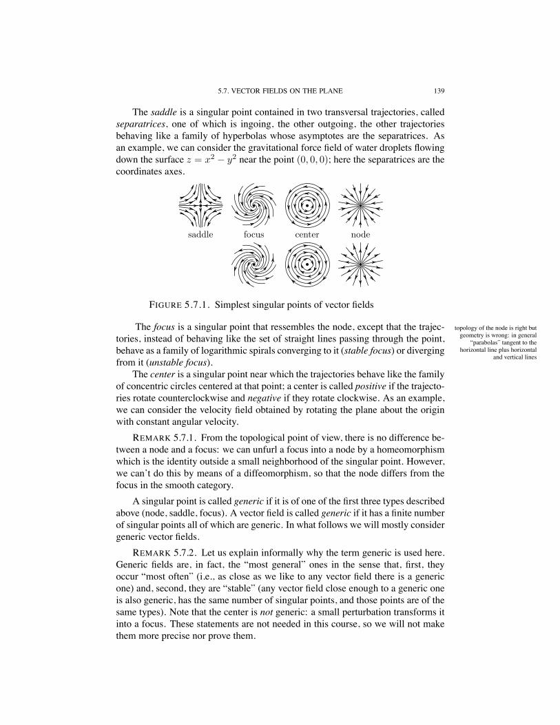
The saddle is a singular point contained in two transversal trajectories, calledseparatrices, one of which is ingoing, the other outgoing, the other trajectoriesbehaving like a family of hyperbolas whose asymptotes are the separatrices. Asan example, we can consider the gravitational force field of water droplets flowingdown the surface z = x2 ' y2 near the point (0, 0, 0); here the separatrices are thecoordinates axes.

saddle focus center node

FIGURE 5.7.1. Simplest singular points of vector fields

The focus is a singular point that ressembles the node, except that the trajec- topology of the node is right butgeometry is wrong: in general

“parabolas” tangent to thehorizontal line plus horizontal

and vertical lines

tories, instead of behaving like the set of straight lines passing through the point,behave as a family of logarithmic spirals converging to it (stable focus) or divergingfrom it (unstable focus).

The center is a singular point near which the trajectories behave like the familyof concentric circles centered at that point; a center is called positive if the trajecto-ries rotate counterclockwise and negative if they rotate clockwise. As an example,we can consider the velocity field obtained by rotating the plane about the originwith constant angular velocity.

REMARK 5.7.1. From the topological point of view, there is no difference be-tween a node and a focus: we can unfurl a focus into a node by a homeomorphismwhich is the identity outside a small neighborhood of the singular point. However,we can’t do this by means of a diffeomorphism, so that the node differs from thefocus in the smooth category.

A singular point is called generic if it is of one of the first three types describedabove (node, saddle, focus). A vector field is called generic if it has a finite numberof singular points all of which are generic. In what follows we will mostly considergeneric vector fields.

REMARK 5.7.2. Let us explain informally why the term generic is used here.Generic fields are, in fact, the “most general” ones in the sense that, first, theyoccur “most often” (i.e., as close as we like to any vector field there is a genericone) and, second, they are “stable” (any vector field close enough to a generic oneis also generic, has the same number of singular points, and those points are of thesame types). Note that the center is not generic: a small perturbation transforms itinto a focus. These statements are not needed in this course, so we will not makethem more precise nor prove them.

140 5. TOPOLOGY AND GEOMETRY OF SURFACES

REMARK 5.7.3. It can be proved that the saddle and the center are not topo-logically equivalent to each other and not equivalent to the node or to the focus;however, the focus and the node are topologically equivalent, as we noted above.

5.7.3. The index of plane vector fields. Suppose a vector field V in the planeis given. Let ' : S1 ! R2 be a closed curve in the plane not passing through anysingular points of V ; denoteC := '(S1). To each vector V (c), c % C, let us assignthe unit vector of the same direction as V (c) issuing from the origin of coordinatesO % R2; we then obtain a map g : C ! S1

1 (where S11 & R2 denotes the unit

circle centered atO), called the Gauss map corresponding to the vector field V andto the curve '. Now we define the index of the vector field V along the curve ' asthe degree of the Gauss map g : S1 ! S1 (for the definition of the degree of circlemaps, see section 5, §3): Ind(', V ) := deg(g). Intuitively, the index is the totalnumber of revolutions in the positive (counterclockwise) direction that the vectorfield performs when we go around the curve once.

REMARK 5.7.4. A simple way of computing Ind(') is to fix a ray issuingfrom O (say the half-axis Ox) and count the number of times p the endpoint ofV (c) passes through the ray in the positive direction and the number of times q inthe negative one; then Ind(') = p' q.

THEOREM 5.7.5. Suppose that a simple closed curve ' does not pass throughany singular points of a vector field V and bounds a domain that also does notcontain any singular points of V . Then

Ind(', V ) = 0 .

PROOF. By the Schoenflies theorem, we can assume that there exists a home-omorphism of R2 that takes the domain bounded by C := '(S1) to the unit diskcentered at the origin O. This homeomorphism maps the vector field V to a vectorfield that we denote by V !. Obviously,

Ind(', V ) = Ind(S10 , V ),

where S1O denotes the unit circle centered at O. Consider the family of all circles

S1r of radius r < 1 centered at O. The vector V !(O) is nonzero, hence for a smallenough r0 all the vectors V !(s), s % S1

r0, differ little in direction from V !(O), so

that Ind(S1r , V ) = 0. But then by continuity Ind(S1

r , V ) = 0 for all r # 1. Nowthe theorem follows from (1). !

Now suppose that V is a generic plane vector field and p is a singular point ofV . Let C be a circle centered at p such that no other singular points are containedin the disk bounded by C. Then the index of V at the singular point p is defined asInd(p, V ) := Ind(C, V ). This index is well defined, i.e., it does not depend on theradius of the circle C (provided that the disk bounded by C does not contain anyother singular points); this follows from the next theorem.