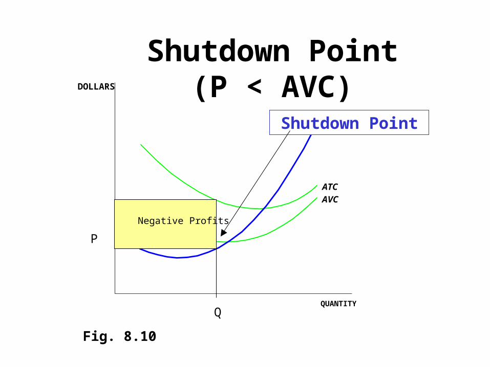
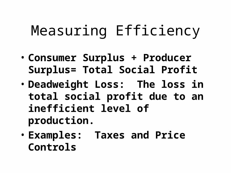
• Consumer Surplus + Producer Surplus= Total Social Profit
• Deadweight Loss: The loss in total social profit due to an inefficient level of production.
• Examples: Taxes and Price Controls
07_07
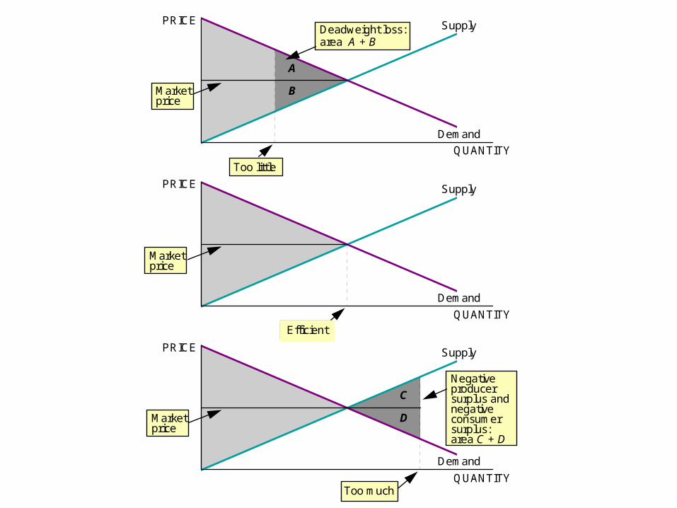
Too little
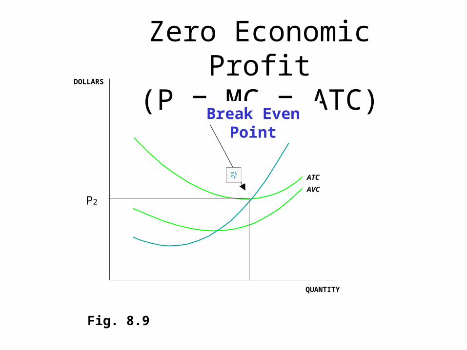
Efficient
QUANTITY
PRICE
Too much
Demand
Supply
C
D
Negative producer surplus and negative consumer surplus: area C + D
QUANTITY
PRICE
Demand
Supply
A
B
QUANTITY
PRICE
Demand
Supply
Deadweight loss: area A + B
Market price
Market price
Market price
Taxation and Deadweight Loss
07_08A
Old supply curve
Demand curve
QUANTITY
PRICE
Deadweight Loss from a Sales Tax
New supply curve
S shifts up by amount of tax
P* Tax RevDWL
CS
PSPp
Pc
Qt Q*
Quantity
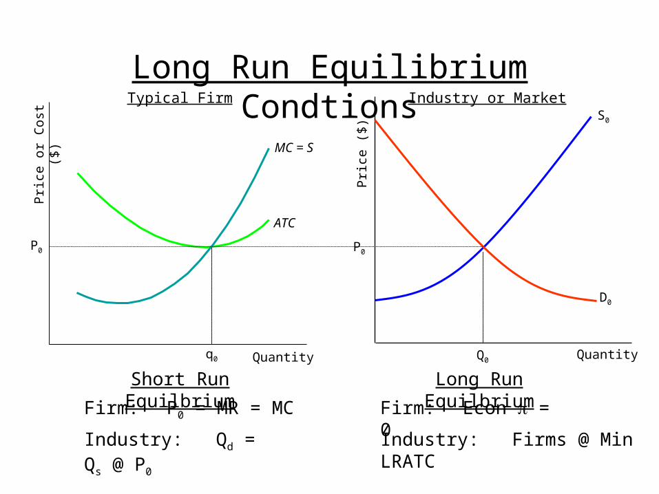
MC = S
ATC
Pri
ce o
r C
ost (
$)
q0
S0
D0
Q0P
rice
($)
Quantity
P0 P0
Typical Firm Industry or Market
Short Run Equilbrium
Firm: P0 = MR = MC
Industry: Qd = Qs @ P0
Long Run Equilbrium
Firm: Econ = 0
Industry: Firms @ Min LRATC
Long Run EquilibriumCondtions
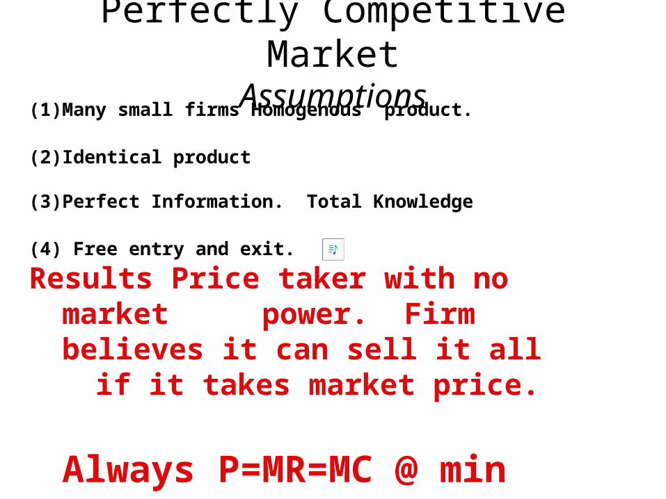
(1) Many small firms Homogenous product.
(2) Identical product
(3) Perfect Information. Total Knowledge
(4) Free entry and exit.
Results Price taker with no market power. Firm believes it can sell it all
if it takes market price.
Always P=MR=MC @ min ATC
Perfectly Competitive MarketAssumptions
Quantity
MC = S
ATC
Pri
ce o
r C
ost (
$)
q0
S0
D0
Q0
Pri
ce (
$)
Quantity
Typical Firm Industry or Market
D1
Q1
P1P1
q1
S1
Long Run Competitive Equilibrium ModelDemand Shock: Shift Demand Left
Loss
Q2q2
P0P2 = P2 = P0
Quantity
MC = S
ATC
Pri
ce o
r C
ost (
$)
q0
S0
D0
Q0
Pri
ce (
$)
Quantity
Typical Firm Industry or Market
D1
Q1
P1P1
q1
S1
Q2q2
P0 P0P2 = P2 =
Long Run Competitive Equilibrium ModelDemand Shock: Shift Demand Right
Profits
Lesson 15 Monopoly: Part 1
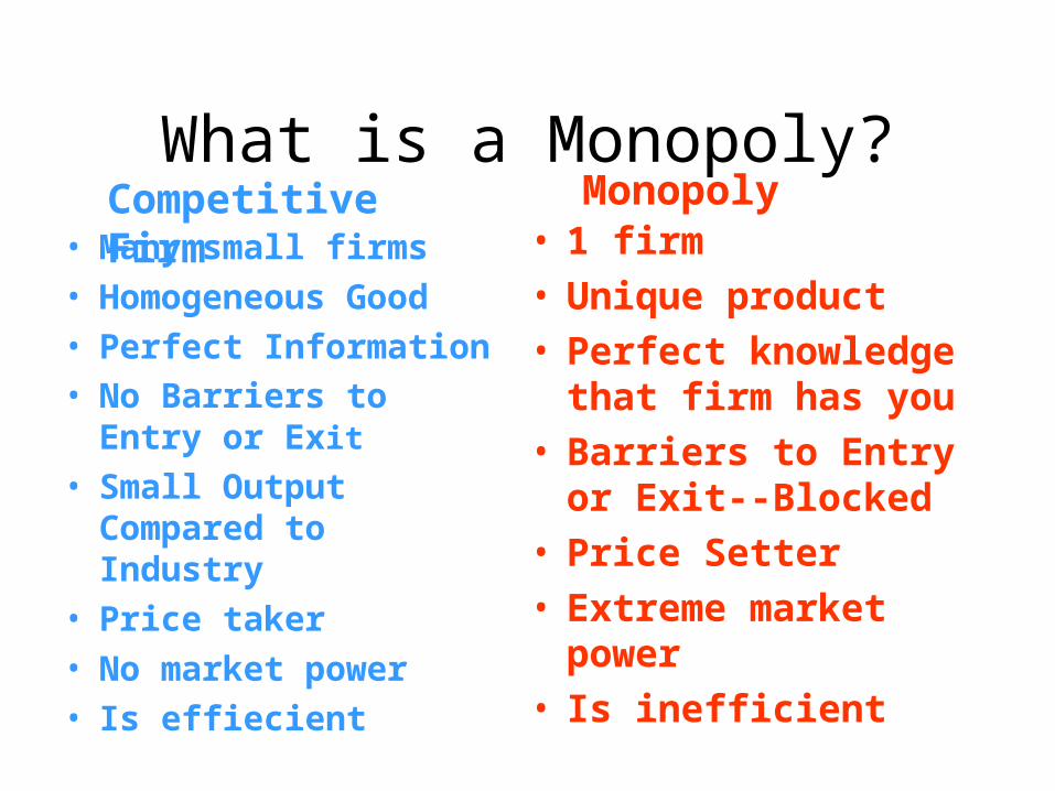
What is a Monopoly?
• Many small firms
• Homogeneous Good
• Perfect Information• No Barriers to Entry or
Exit
• Small Output Compared to Industry
• Price taker
• No market power
• Is effiecient
• 1 firm • Unique product• Perfect knowledge that
firm has you• Barriers to Entry or
Exit--Blocked• Price Setter• Extreme market power• Is inefficient
Competitive Firm Monopoly
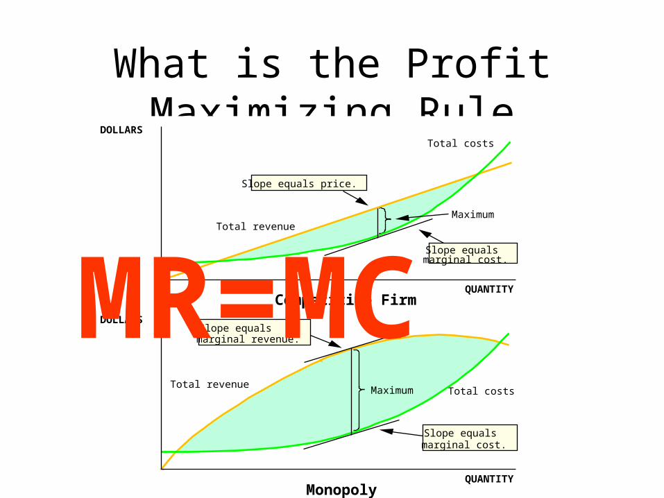
What is the Profit Maximizing Rule
10_05
Total costs
Total costs
Total revenue
Total revenue
Maximum
Maximum
QUANTITY
DOLLARS
Slope equals price.
Slope equals marginal cost.
QUANTITY
DOLLARS
Competitive Firm
Monopoly
Slope equals marginal revenue.
Slope equals marginal cost.
MR=MC
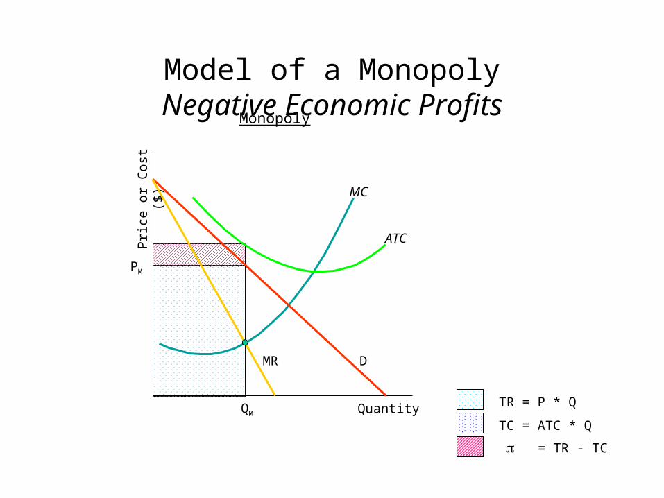
TR = P * Q
= TR - TC
TC = ATC * QQuantity
MC
ATC
Pri
ce o
r C
ost (
$)
Monopoly
DMR
QM
PM
Model of a MonopolyPositive Economic Profits
TC = ATC * Q
TR = P * QQuantity
MC
ATCPri
ce o
r C
ost (
$)
Monopoly
QM
PM
= TR - TC
DMR
Model of a MonopolyNegative Economic Profits
Model of a Monopoly Board Problem
Market: Cadet Comforters Scenario: QD = 40 - P where Q: comforters / week
TC = Q2 + 4Q + 58 P: $ / comforter
Question: (a) Calulate the MR and MC functions.
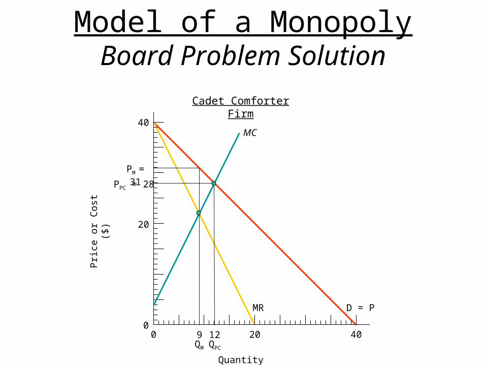
(b) Depict the following curves on a graph: D, MR, MC.
(c) Determine the equilibrium price and quantity if the firm acts like a perfectly competitive firm. Depict PPC and QPC on the graph. Calculate the firm’s profits.
(d) Determine the equilibrium price and quantity if the firm acts like a monopoly. Depict PM and QM on the graph. Calculate the firm’s profits.
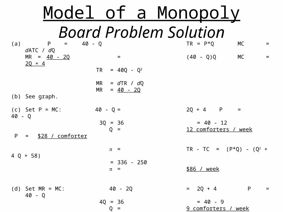
Model of a MonopolyBoard Problem Solution
(a) P = 40 - Q TR = P*Q MC = dATC / dQMR = 40 - 2Q = (40 - Q)Q MC = 2Q + 4
TR = 40Q - Q2
MR = dTR / dQMR = 40 - 2Q
(b) See graph.
(c) Set P = MC: 40 - Q = 2Q + 4 P = 40 - Q 3Q = 36 = 40 - 12 Q = 12 comforters / week P = $28 / comforter