2.1 Interaction Between Light and Matter ___________________________________________ 8 2.1.1 Gas Absorption ___________________________________________________________________ 8 2.1.2 Thermal Self-Emission ____________________________________________________________ 16 2.1.3 Atmospheric Considerations and Simulation ___________________________________________ 18 2.1.4 Self-emission in the MWIR (night) and LWIR _________________________________________ 20 2.1.5 Self-emission in the MWIR (day) ____________________________________________________ 22
3 Stochastic Modeling ______________________________________________________ 24 3.1 Probability Theory: Random Variables _________________________________________ 25
3.2 Probability Theory: Random Fields ____________________________________________ 26
3.3 Probability Theory: Correlation Measures ______________________________________ 26
3.4 Random Fractal Theory ______________________________________________________ 27 3.4.1 Fractional Brownian Motion ________________________________________________________ 27 3.4.2 Spectral Density _________________________________________________________________ 28
6.2 3D-DDA ____________________________________________________________________ 60 6.2.1 Ray Tracing Gas Clouds in DIRSIG __________________________________________________ 62
13 Appendix D: Adding Spectral Noise in ENVI ________________________________ 107 13.1 Adding Spectral Noise Using EigenVector-Based Transforms ____________________ 107
13.2 Adding Spectrally Correlated Noise Using a Dark Current Image ________________ 110
13.3 Adding Spectrally Correlated Noise Without a Dark Current Image ______________ 114
14 Appendix E: Design Experiment for Truth Data Via a Benign Gas ______________ 116 14.1 Design Outline ___________________________________________________________ 116
The capability to digitally model and simulate chemical weapon (CW) clouds is crucial in the
development of detection methods designed to keep military and civilian personnel well away
from chemical weapon release. Both the release and modeling of CW clouds covers a broad
range of complex phenomena. The manner in which the CW is released, the terrain over which
it travels, surrounding buildings, initial momentum, seasonal variations, possible canopy
structure, atmospheric pressure, environmental parameters such as solar insolation, rain, and
wind speed all effect the evolution of the gas cloud. This research concentrated only on a small
portion of the much larger picture. The main goal was to provide a simple model that predicts
the dispersion, advection, dissipation, concentration, and temperature with respect to time of
these deadly clouds. Potential improvements to the model will be discussed in the section titled:
Conclusion and Improvements.
The CWs of interest in this research are known as nerve agents. All nerve agents in their pure
state are colorless liquids at STP. Nerve agents inhibit the release of the enzyme
acetylcholinesterase. This affects nerve impulses causing severe muscle cramping and death by
suffocation. All nerve agents belong to the chemical group of organo-phosphorus compounds.
They are stable and easily dispersed, highly toxic and have rapid effects (2-30 minutes) when
absorbed though the skin and via respiration. [ICA, 1997]
Nerve agents are typically disseminated in three manners. The first is to use a burster or binary
technology (3-7 kg). Two liquid components are separated in a projectile by a rupture disc.
When the projectile is fired the disc bursts and the two components combine. Rifling in the
barrel gives the projectile a spinning velocity that mixes the nerve agent. The second method is
to mix the components before launch and store them in a ballistic missile warhead (200-1000
kg). The third is to let the agent leak out and be dispersed by the air stream. This research
concentrates on discrete sources and is applicable mainly to binary and warhead dissemination.
6
However, continuous sources can be treated as discrete sources that are closely placed together.
Therefore any number of continuous source plume models could be used to model the third case
scenario.
Spectral data was supplied through the Army’s Aberdeen Proving Grounds for the following
nerve agents: VX , Distilled Mustard (HD), Soman (GD), Sarin (GB), and Tabun (GA). The
spectral features for these nerve agents are in the mid-wave (MWIR) to long wave infrared
(LWIR), 4-24µm. In this region the primary sources of radiance reaching the sensor are thermal
self-emission, upwelled thermal emission, background thermal emission, and earth thermal
emission. The self-emission of the gas is dependent on the temperature and emissivity of the
gas. The transmission of the gas will be dependent on the spectral absorbence of the nerve agent.
Scattering is ignored since it is considered negligible above 2.5µm. [Kuo, 1997]
In this research, synthetic image generation (SIG) was used to simulate the CW clouds and
investigate remote sensing capabilities in detection. The simulations were run using Soman
(GD) although any of the nerve agents could have been used. SIG uses first principles from
physics to produce radiometrically accurate images as seen by a sensor. SIG allows the user to
vary scene and sensor geometries, wavelengths, meteorological conditions, background
interactions, and atmospheric profiles without the need for dangerous and expensive field
releases.
The rendering of these synthetic scenes will be done with the Digital Imaging and Remote
Sensing Image Generation (DIRSIG) code. DIRSIG is a ray tracing code developed by the
Digital Imaging and Remote Sensing lab (DIRS) at the Center for Imaging Science at the
Rochester Institute of Technology in Rochester, NY. It creates radiometrically accurate
synthetic images for various sensor platforms [Brown, 1999]1. DIRSIG incorporates the
Moderate Resolution Transmittance (MODTRAN) code [Berk, 1989] to model the atmosphere.
To support the higher spectral resolution needed on this effort, the Fast Atmospheric Signature
Code (FASCODE) [Smith, 1978] was added as a source of atmospheric parameters. The points
of contact, general descriptions, documentation references, and software downloads for both
7
MODTRAN and FASCODE are available at http://www-vsbn.plh.af.mil. The THERM [DCS
Corporation, 1990] thermal sub-model is incorporated in DIRSIG to predict time dependent
temperatures of objects within the scene as influenced by their environment.
The simulation of a time sequence depicting the evolution of a CW cloud is quite complex and
requires modeling capabilities that are still evolving. This type of simulation is known as
physical dynamic modeling. The user does not specify the entire phenomenon, but rather
provides external forces and material properties. The model then predicts the evolution of the
position and shape of the gas over time based on physics. The model presented in this research
draws from theory used in the morphology of smoke plumes [Beychok, 1994 & Blackadar,
1997]. The forms that smoke plumes exhibit are a result of diffusion and atmospheric turbulence
due to heating currents and wind deviations. Knowledge based on measurements acquired over a
long period have been used to successfully predict smoke plume movement. Traditionally these
smoke plume models use Fickian Diffusion that predicts a concentration with a Gaussian or
Normal probability distribution function (PDF). The Fick equation states that the rate of change
of the concentration of a property depends on the divergence of the three-dimensional flux of the
property, and that in an inhomogeneous environment the flux is proportional to the gradient of
the mean concentration. The Gaussian shape of predicted plumes and clouds is consistent with
most experimental data if sufficient allowance is given to sampling irregularities [Blackadar,
1997]. This technique describes the macroscopic properties or global shape of the gas cloud. A
fractional Brownian motion (fBm) field is then introduced to add turbulent small-scale detail.
Fractional Brownian motion can be used to describe the irregular thermal motion of the gas
molecules and fits under the concept of fractal geometry [Crownover, 1995].
At this time a blast model is not available. A blast model would help in developing the initial
kinetic theory describing the evolution of the gas until some equilibrium was reached at some
time, t2 > 0. The model presented in this research describes the evolution after reaching
equilibrium, t2.
1 Download available from http://www.cis.rit.edu/~dirsig/doc/index.html
8
2 Radiation Propagation
This section discusses the basic physics involved with quantifying the radiance from target to
sensor. This covers the interaction between light and matter and the radiometric equations
involved with the remote sensing of gas clouds.
2.1 Interaction Between Light and Matter
2.1.1 Gas Absorption
Different gasses attenuate light at various wavelengths. These absorption features can be used as
"finger prints" which can identify the gas. The field of identifying these "finger prints" is known
as spectroscopy. The intensity and shape of these lines are a function of temperature, molecular
weight of the gas concentration, and relative pressure. One important spectral broadening
process is caused by the Doppler effect, in which radiation is shifted in frequency when the
source is moving towards or away from the observer. Doppler theory states that frequency
increases with temperature and decreases with molecular mass according to:
Δv∝ TMW
Equation 2-1
where Δv = width of absorption frequency, T = Temperature [Kelvin], MW = gram
molecular weight [g/mol]
The degree of broadening is also proportional to the relative pressure [Schott, 1997]. In the
MWIR these absorption lines are due to transitions in the vibrational state of the molecule.
Above 20 µm rotational transitions are the dominant process. Figure 2-1 illustrates an idealized
absorption spectra. Figure 2-1b demonstrates the effects of broadening caused by temperature,
9
pressure, and molecular weight. Figure 2-1c represents the net effect of overlap between the
broadened spectra. Thus, discrete absorption features can be lost due to overlap caused by
broadening.
6(a) Idealized absorption spectra
0
(b) Effects of broadening isolated for each of the lines shown in (a)
0
1
0
(c) Cumulative absorption spectra
1
1
Absorption
Wavelength
h
h
h
Figure 2-1 Characteristics of absorption spectra [Schott, 1997]
For a more rigorous treatment of absorption and remote sensing see Goody (1989).
The following is from Schott [1997]:
In simplified form, we can derive the following relationships between the number and efficiency of absorbers and their effect on the propagating beam. At each wavelength, we define the absorption cross section Cα to be the effective size of a
10
molecule relative to the photon flux at that wavelength. Conceptually, this can be expressed as:
Cα = Cgξ = πr2ξ [m2 ]
Equation 2-2
where Cg [m2] is the geometric cross section for a molecule of radius r [m] and ξ is a unitless wavelength-dependent efficiency factor that is proportional to the molecule’s ability to absorb flux. Values of Cα can be derived for particular temperatures and pressures from experimental data or through molecular energy theory, then adjusted for the effects of the temperature and pressure. The molecule is then assumed to be a perfect absorber over that cross-sectional area. To compute the fractional amount of energy lost per unit length of transit in a propagating beam, we need to know the number density of the molecules. Referring to Figure 2-2, we let m´ be the number of molecules in a unit volume of side dimension l[m].
Molecule with absorption cross section C_
l [m] length of each side of the unit volume
(a) A unit volume containing m’ absorption centers. We assume that the medium has a large mean free path such that in a small volume, if we project the molecules onto one face, there will be no overlap, i.e.,
(b) Projection of absorbers onto the face of the volume
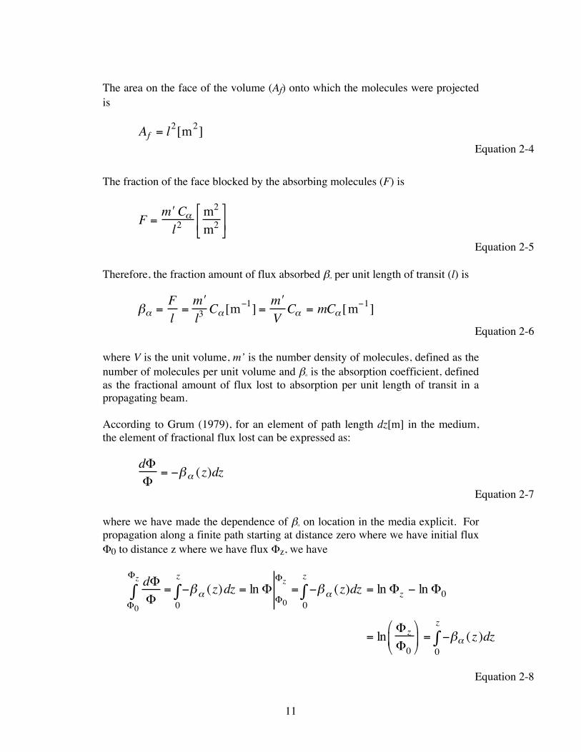
Figure 2-2 Computation of the absorption coefficient [Schott, 1997] Then, the area blocked (Ab) by the molecules is Ab = m! Cα [m
2 ] Equation 2-3
11
The area on the face of the volume (Af) onto which the molecules were projected is Af = l
2[m2] Equation 2-4
The fraction of the face blocked by the absorbing molecules (F) is
F =m!Cαl2
m2
m2#
$ %
&
' (
Equation 2-5 Therefore, the fraction amount of flux absorbed βα per unit length of transit (l) is
βα =Fl=m#l3Cα [m
−1] = m#VCα = mCα [m
−1] Equation 2-6
where V is the unit volume, m’ is the number density of molecules, defined as the number of molecules per unit volume and βα is the absorption coefficient, defined as the fractional amount of flux lost to absorption per unit length of transit in a propagating beam. According to Grum (1979), for an element of path length dz[m] in the medium, the element of fractional flux lost can be expressed as:
dΦΦ
= −βα (z)dz
Equation 2-7 where we have made the dependence of βα on location in the media explicit. For propagation along a finite path starting at distance zero where we have initial flux Φ0 to distance z where we have flux Φz, we have
dΦΦ
= −βα (z)dz = lnΦΦ0
Φz= −βα (z)dz0
z
∫0
z
∫Φ0
Φz
∫ = lnΦz − lnΦ0
= ln Φ zΦ0
&
' (
)
* + = −βα (z )dz
0
z
∫
Equation 2-8
12
Making both sides powers of e to simplify the left-hand side yields
ΦzΦ0
= e− βα (z )dz0
z∫
Equation 2-9
Recognizing the left-hand side as a definition of transmission (ratio of flux out to flux in) and solving for the simplified case of a homogeneous medium, we have
τ =ΦzΦ0
= e−βα dz
0
z∫
= e−βα z
Equation 2-10
which is variously known as Lambert’s law or Bouguer’s law. The product βαz is generally referred to as the optical depth (δ), i.e., δa = βα z
Equation 2-11
To this point we have implicitly assumed a media containing a single constituent. For a homogeneous media containing many types of molecules, we introduce the subscript i to denote the particular constituent. If we assume that the molecules interact independently with the propagating flux, we can express the transmission as: τ = τi∏ = e− δi∑ = e− β αi z∑ = e− miCα iz∑ = e−βα z = e−δ a
Equation 2-12
where Π designates the product of the transmission values for each constituent if computed separately, the summation (Σ) is over all constituents, and we redefine βα =Σβαi to be the composite absorption coefficient and δi to be the composite optical depth due to absorption. [Schott, 1997]
Finally the relationship between absorption and transmission is expressed as:
A = -ln(τ)
Equation 2-13
13
The spectral absorption "finger print" is a function of the absorption coefficient, concentration of
the gas, and the path-length over which the absorption was measured. The raw data was
provided through the Army's Aberdeen Proving Grounds, MD. For published data see Hoffland
(1985). The raw data provided units of absorption coefficients in liters/(gram*cm),
concentration in grams/liter, and path-length in meters. To determine absorption from Bouguer's
Law:
A = βαCz
Equation 2-14
Where βα= absorption coefficient [L/g*cm], C = concentration [g/L], and z = path-length of the
cell [m]
The concentration of gases is often given in parts per million [ppm] and is known as the volume-mixing ratio (VMR). The definition of 1 ppm of a gas means there is one part of gas per 1 million parts of air. The VMR can be computed through the following derivation:
molar density [mol/L] = concentration [g/L]
molecular weight [g/mol]
Equation 2-15
molar density [molm3 ] = molar density [
molL
] * 1000[L]1[m3]
Equation 2-16
VMR [ppm] = molar density [molm3 ]* 0.0224volume of ideal gas @ STP[ m3
mol]
*1000000
Equation 2-17
A similar conversion is needed to convert the absorption coefficient to 1/ppm-m:
14
1[m]100[cm]*
1000000 * ]molmP[ volume@STgas normal 0.0224,
1000[L]]1[m*]
molgwt[molecular *]
cm*gL[
]m-ppm
1[ 3
3
α
α
ββ =
Equation 2-18
STP stands for standard temperature (273.15 K) and pressure (1 ATM). The gas volume can be
adjusted for various temperatures and pressures by using the ideal gas law:
Gas Volume [m3
mol] =
R [L *atmmol* K
]∗T[K]
P [atm]∗
[m3 ]1000[L]
Equation 2-19
Where R = Universal gas constant = kNa = Boltzmanns's constant*Avogadro's number =
8.2057e-2 [L*atm/mol*K], T = temperature [K], and P = pressure [atm].
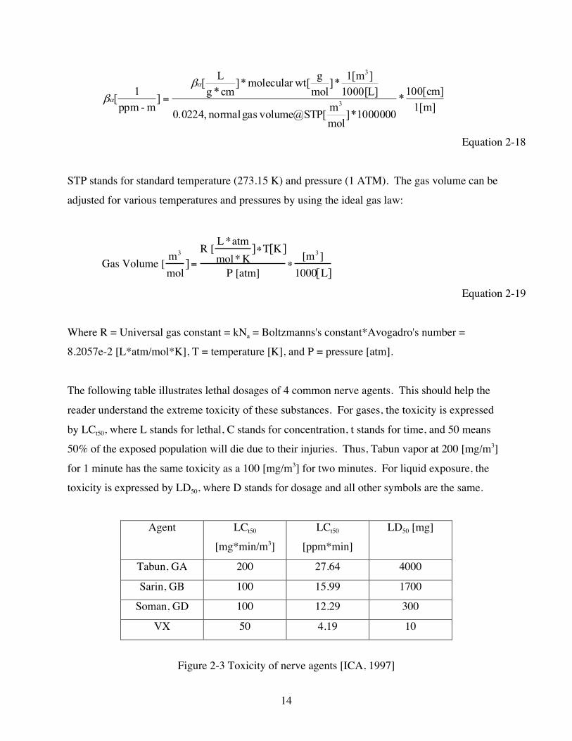
The following table illustrates lethal dosages of 4 common nerve agents. This should help the
reader understand the extreme toxicity of these substances. For gases, the toxicity is expressed
by LCt50, where L stands for lethal, C stands for concentration, t stands for time, and 50 means
50% of the exposed population will die due to their injuries. Thus, Tabun vapor at 200 [mg/m3]
for 1 minute has the same toxicity as a 100 [mg/m3] for two minutes. For liquid exposure, the
toxicity is expressed by LD50, where D stands for dosage and all other symbols are the same.
Agent LCt50
[mg*min/m3]
LCt50
[ppm*min]
LD50 [mg]
Tabun, GA 200 27.64 4000
Sarin, GB 100 15.99 1700
Soman, GD 100 12.29 300
VX 50 4.19 10
Figure 2-3 Toxicity of nerve agents [ICA, 1997]
15
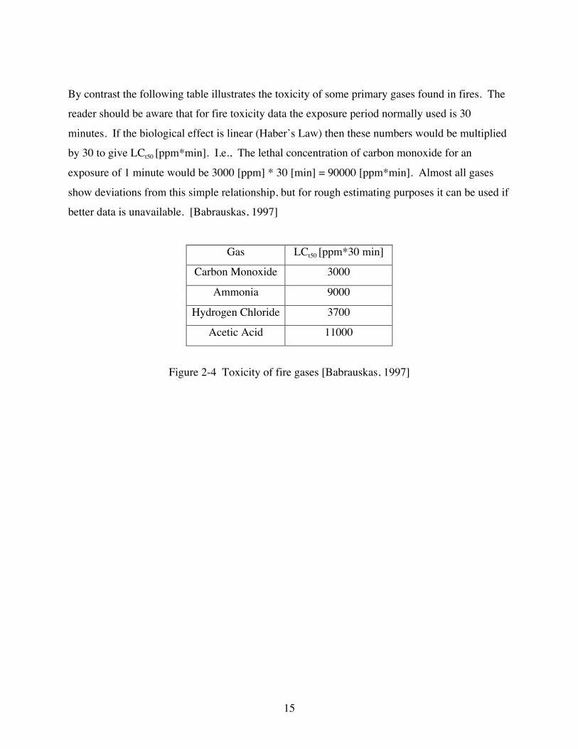
By contrast the following table illustrates the toxicity of some primary gases found in fires. The
reader should be aware that for fire toxicity data the exposure period normally used is 30
minutes. If the biological effect is linear (Haber’s Law) then these numbers would be multiplied
by 30 to give LCt50 [ppm*min]. I.e., The lethal concentration of carbon monoxide for an
exposure of 1 minute would be 3000 [ppm] * 30 [min] = 90000 [ppm*min]. Almost all gases
show deviations from this simple relationship, but for rough estimating purposes it can be used if
better data is unavailable. [Babrauskas, 1997]
Gas LCt50 [ppm*30 min]
Carbon Monoxide 3000
Ammonia 9000
Hydrogen Chloride 3700
Acetic Acid 11000
Figure 2-4 Toxicity of fire gases [Babrauskas, 1997]
16
2.1.2 Thermal Self-Emission
The emissivity characterizes the radiating efficiency of a surface and is material dependent. It is
a unitless number with range 0 -> 1, with 1 being a perfect emitter. According to the second law
of thermodynamics the rate of emission at a given wavelength must equal the rate of absorption
at that wavelength. Thus, all of the incident radiation on the ideal emitter would be absorbed.
Since no radiation is reflected from the surface an ideal emitter is often called a blackbody.
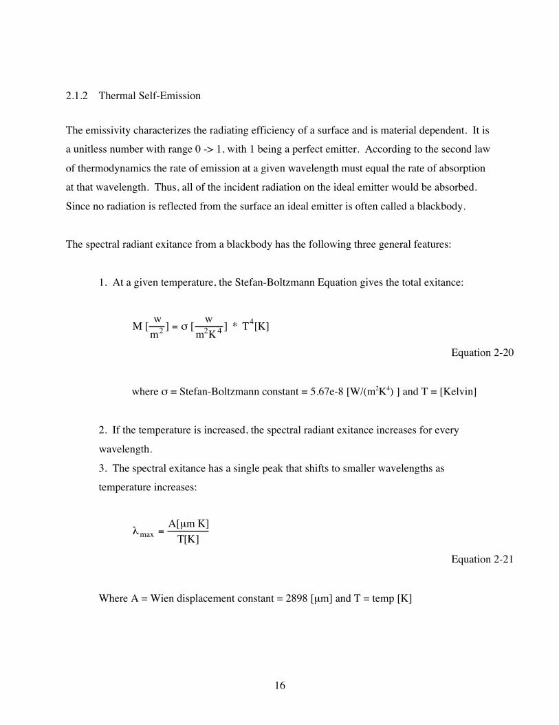
The spectral radiant exitance from a blackbody has the following three general features:
1. At a given temperature, the Stefan-Boltzmann Equation gives the total exitance:
M [ wm2 ] = σ [ w
m2K 4 ] * T4[K]
Equation 2-20
where σ = Stefan-Boltzmann constant = 5.67e-8 [W/(m2K4) ] and T = [Kelvin]
2. If the temperature is increased, the spectral radiant exitance increases for every
wavelength.
3. The spectral exitance has a single peak that shifts to smaller wavelengths as
temperature increases:
λmax =A[µm K]
T[K]
Equation 2-21
Where A = Wien displacement constant = 2898 [µm] and T = temp [K]
17
As a function of wavelength the Planck Equation expresses the spectral radiant exitance from a
blackbody:
m)][W/(m 1) - (
hc2 )M( 2
5
2
bb µλ
πλ
λTKhc
e=
Equation 2-22
Where λ = wavelength [µm], h = Plank's constant 6.6256e-34 [joules sec], c = speed of light 3e8
[m/s], T = temp [K], K = Boltzmann gas constant 1.38e-23[joules/K]
The Planck equation can be expressed in terms of spectral radiance for Lambertian surfaces as:
]msr m
w [ ) M( = )( 2 µπλ
λL
Equation 2-23
The emissivity is then defined as:
ε(λ) =M(λ, T)Μ bb(λ,Τ)
, 0 < ε(λ) <1
Equation 2-24
Where M(λ,Τ) = radiant exitance of an object at a given wavelength and temperature and
Mbb(λ,Τ) = radiant exitance of a blackbody at the same wavelength and temperature.
For a gas volume the emissivity can be expressed as a function of the transmission loss due to
absorption as:
ε(λ) = 1 − τ(λ) = 1− e-Kabsz
Equation 2-25
18
Where τ(λ)= transmittance and ε(λ) = emissivity
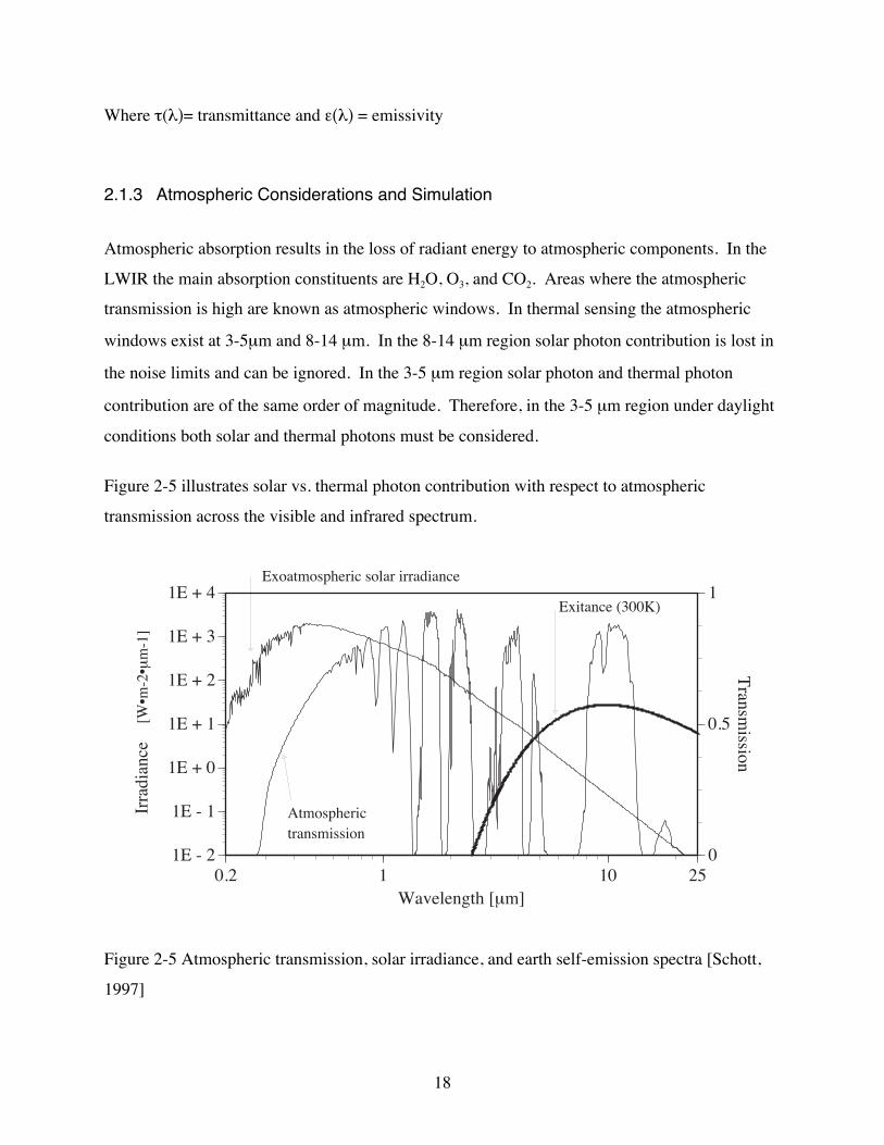
2.1.3 Atmospheric Considerations and Simulation
Atmospheric absorption results in the loss of radiant energy to atmospheric components. In the
LWIR the main absorption constituents are H2O, O3, and CO2. Areas where the atmospheric
transmission is high are known as atmospheric windows. In thermal sensing the atmospheric
windows exist at 3-5µm and 8-14 µm. In the 8-14 µm region solar photon contribution is lost in
the noise limits and can be ignored. In the 3-5 µm region solar photon and thermal photon
contribution are of the same order of magnitude. Therefore, in the 3-5 µm region under daylight
conditions both solar and thermal photons must be considered.
Figure 2-5 illustrates solar vs. thermal photon contribution with respect to atmospheric
transmission across the visible and infrared spectrum.
1E - 2
1E - 1
1E + 0
1E + 1
1E + 2
1E + 3
1E + 4
0
0.5
1
0.2 1 10 25
Irrad
ianc
eTransm
ission
Wavelength [µm]
Exoatmospheric solar irradiance
Atmospheric transmission
Exitance (300K)
[W•m
-2•µ
m-1
]
Figure 2-5 Atmospheric transmission, solar irradiance, and earth self-emission spectra [Schott,
1997]
19
Figure 2-5 shows the selection of a sensor must consider the atmospheric window, spectral
sensitivity of the sensor, along with source, magnitude, and spectral composition of the photons
available [Lillesand, 1994]. For the work reported here, solar and self emmisive calculations are
included at all wavelengths, however, scattering effects in the gas plume are not included.
Scattering is typically insignificant in the MWIR and LWIR and should not introduce any
significant errors when the cloud droplets are small compared with the imaging wavelength.
The atmosphere will be modeled using the atmospheric transport code MODTRAN for delta
wave number increments > 2 [cm-1]. This program is a computationally rigorous radiation
transfer algorithm that models the spectral absorption, transmission, emission, and scattering
characteristics of the atmosphere. MODTRAN assumes that the atmosphere is a set of
homogeneous layers. The characteristics of these layers are either modeled by several default
model atmospheres or it can be characterized by radiosonde data collected for a specific
atmosphere. In the regions of interest for this research (8-14µm and 3-5µm at night) where solar
photons are ignored, the radiance reaching the sensor can be approximated by:
Lλ = εLTλ τiλi=1
N∏ + (1− τ iλ )LTiλ τ jλ
j=i+1
N∏
&
' (
)
* +
i=1
N∑
Equation 2-26
Where τiλ = transmission through the ith layer along a path length zi at wavelength λ, LTiλ=
blackbody spectral radiance with temperature Ti of the ith layer.
High resolution runs, for wave numbers < 2 [cm-1], used FASCODE. This model is a line-based
method versus MODTRAN band-based method.
The next two sections cover the thermal governing equations for remote sensing of gaseous
clouds.
20
2.1.4 Self-emission in the MWIR (night) and LWIR
Thermal sources are the significant contributors in the MWIR (at night) and LWIR. The
radiance reaching the sensor is a function of Planck's Equation, Equation 2-22, modified by the
emissivity as a function of wavelength, defined as one minus the transmission, Equation 2-25.
The primary sources of interest are: gas cloud self-emission (LSε), upwelled thermal radiance
The thermal radiance reaching the sensor without the gas cloud can be expressed as:
21
εεεε
εεεε
τπ
ε U2d
BDE
UBDE
Lr))F1(F(L
LLL+ LL
+⎥⎦
⎤⎢⎣
⎡−++=
++=
EE
Equation 2-27
Where rd = diffuse reflectance (constant at all angles), τ2 = transmission from target to sensor, F
= shape factor, and E = irradiant [w/m2]
The earth self-emission term (Eε) dominates this expression with significant contribution from upwelled radiance (Uε). The reflected downwelled radiance (Dε) and reflected background radiance (Bε) terms are typically much smaller, though still significant contributors if measurement accuracy’s of tenths of a degree are desired. The relative importance of these reflected terms will decrease with increasing emissivity (decreasing reflectivity), but in general they will not be negligible until emissivity values approach 0.99. The relative importance of the downwelled radiance and the background radiance is controlled by the shape factor (F). The shape factor represents the fraction of hemisphere above the target that is sky. For nearly horizontal unobstructed surfaces, the shape factor F approaches 1.0 and the background term becomes negligible. [Schott, 1997]
The temperature of the gas cloud will determine the blackbody exitance as expressed by Planck's
Equation, Equation 2-22. The blackbody exitance multiplied by the emissivity as a function of λ
determines the gas cloud self-emission. In simple form this can be approximated as:
ggC )L - (1 L Tτε =
Equation 2-28
Where τg = effective transmittance of the gas and Lt. = radiance due to the temperature of the gas
[W/(m2*sr)]
Equation 2-27 with the gas cloud then becomes:
εεεε τττπ
ε Uggg2d
BDE L)L - (1 r))F1(F(LL ++⎥⎦
⎤⎢⎣
⎡−++= TEE
Equation 2-29
22
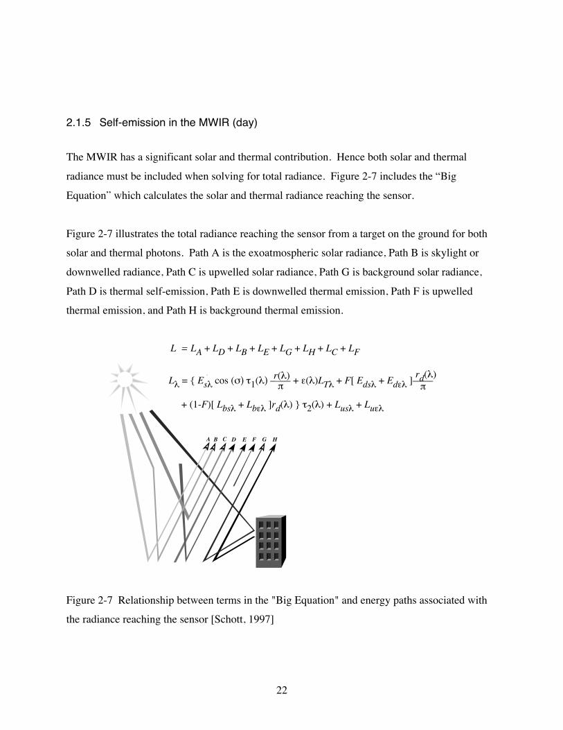
2.1.5 Self-emission in the MWIR (day)
The MWIR has a significant solar and thermal contribution. Hence both solar and thermal
radiance must be included when solving for total radiance. Figure 2-7 includes the “Big
Equation” which calculates the solar and thermal radiance reaching the sensor.
Figure 2-7 illustrates the total radiance reaching the sensor from a target on the ground for both
solar and thermal photons. Path A is the exoatmospheric solar radiance, Path B is skylight or
downwelled radiance, Path C is upwelled solar radiance, Path G is background solar radiance,
Path D is thermal self-emission, Path E is downwelled thermal emission, Path F is upwelled
thermal emission, and Path H is background thermal emission.
Figure 2-7 Relationship between terms in the "Big Equation" and energy paths associated with
the radiance reaching the sensor [Schott, 1997]
23
All paths in Figure 2-7 are included in the DIRSIG simulations. In addition a gas cloud will
attenuate both thermal and solar photons and emit thermal photons as discussed in section 6.2.1.
Because the focus is on the MWIR and LWIR where scattering is typically low, scattering effects
from the gas cloud are not included. This should not introduce any significant errors when the
cloud is very gaseous, i.e. gas droplets are small relative to imaging wavelength. However, if a
significant number of droplets or large particles are associated with the cloud then scattering
should be considered for future upgrades.
The previous sections lay down the physics (the “Big equation”) involved with quantifying the
energy emitted and absorbed by a gas cloud. They also discuss the energy contributions from
background and atmospheric interactions. The sections propose ways to calculate and quantify
various sources in order to model what the sensor will detect as they relate to certain atmospheric
window constraints. The reader should keep in mind that DIRSIG and MODTRAN or
FASCODE are used as the primary tools to model the physics discussed in the previous sections.
24
3 Stochastic Modeling
Convective atmospheric transport and diffusion effects on aerosol concentrations in plumes can
be represented with a Gaussian distribution. This Gaussian model visualizes aerosol plumes as
smooth distributions resulting from time-averaged contributions of turbulence to the mean flow.
Any observer of aerosol plumes knows that the distribution is not perfectly Gaussian but has
some random behavior. The behavior of a probabilistic system cannot be predicted exactly but
the probability of certain behaviors is known. Fractals and mathematical chaos lay the
foundation for numerical techniques that can be used to generate spatially correlated random
fields. The fluctuations that occur with chaos sets are only seemingly random. This pseudo-
randomness spawns from a sensitive dependence on initial conditions. The input parameters
introduce some error or randomness but the overall process follows some deterministic outcome.
Fractal statistics are used to generate superpositions of random fluctuations over different time
scales. This randomness can be used to simulate turbulence. As pointed out by Sakas (1993);
Mandelbrot (1975) and Lovejoy (1985) proposed that static images of turbulent fields can be
regarded as fractals with a Hurst exponent of 0.7. This corresponds closely to experimental
values of actual turbulence measured by Sreenivasan (1991).
The following sections attempt to describe a family of random fractal functions known as
fractional Brownian motion (fBm). FBm has been used in many applications ranging from
physical sciences and engineering to artistic applications. For a more in-depth discussion of
fractals, chaos, and fBm see Tompson (1989), Crownover (1995), and Yaglom (1986). The
following heuristic arguments are taken from Stam (1991 & 1995) and Peitgen (1988).
25
3.1 Probability Theory: Random Variables
The set of all possible outcomes for a given observation is called the sample space. A random
variable X or in general the variate X is a variable that can take on any value in the sample space.
The overall behavior of a random variate X can be described by its probability distribution
function (PDF). The PDF is a function P[X=x] meaning "the probability of variate X equal to x"
defined by:
pdf = f(x)dx = 1, −∞
∞
∫ 0 ≤ f(x) ≤1
Equation 3-1
In practice, the statistics of the random variate X are used to provide useful information. These
statistics include the expectation or mean, standard deviation, variance, and correlation. The
mean is defined as:
µ = E[x]= xf(x)dx−∞
∞
∫
Equation 3-2
The variance is a measure of how the values X are distributed around the mean:
2222
-
2 -]E[x ])-E[(x dx )x(f)-(x=Var[x] µµµσ === ∫∞
∞
Equation 3-3
26
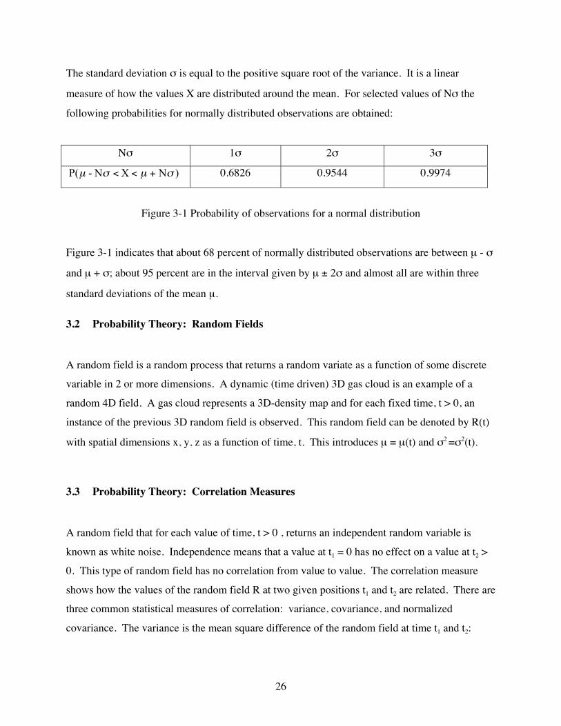
The standard deviation σ is equal to the positive square root of the variance. It is a linear
measure of how the values X are distributed around the mean. For selected values of Nσ the
following probabilities for normally distributed observations are obtained:
Nσ 1σ 2σ 3σ
)N X N - P( σµσµ +<< 0.6826 0.9544 0.9974
Figure 3-1 Probability of observations for a normal distribution
Figure 3-1 indicates that about 68 percent of normally distributed observations are between µ - σ
and µ + σ; about 95 percent are in the interval given by µ ± 2σ and almost all are within three
standard deviations of the mean µ.
3.2 Probability Theory: Random Fields
A random field is a random process that returns a random variate as a function of some discrete
variable in 2 or more dimensions. A dynamic (time driven) 3D gas cloud is an example of a
random 4D field. A gas cloud represents a 3D-density map and for each fixed time, t > 0, an
instance of the previous 3D random field is observed. This random field can be denoted by R(t)
with spatial dimensions x, y, z as a function of time, t. This introduces µ = µ(t) and σ2 =σ2(t).
3.3 Probability Theory: Correlation Measures
A random field that for each value of time, t > 0 , returns an independent random variable is
known as white noise. Independence means that a value at t1 = 0 has no effect on a value at t2 >
0. This type of random field has no correlation from value to value. The correlation measure
shows how the values of the random field R at two given positions t1 and t2 are related. There are
three common statistical measures of correlation: variance, covariance, and normalized
covariance. The variance is the mean square difference of the random field at time t1 and t2:
27
γ (t1,t 2 ) =12Ε[(R(t1) − R(t2 ))
2 ]
Equation 3-4
The covariance is:
Cov(t1, t2 ) = E[R(t1 )R(t2 )] - µ(t1)µ(t 2 )
Equation 3-5
Positive values of the covariance indicate values of the random field tend to be close. Negative
values indicate a large difference in values. The normalized covariance or correlation function is
:
Cor(t1,t 2 ) =Cov(t1,t 2 )σ(t1)σ(t2 )
Equation 3-6
All these basic functions are used to describe the statistics of the random field.
3.4 Random Fractal Theory
3.4.1 Fractional Brownian Motion
In one dimension fBm, BH(t), is a single valued function of time, t. Its increments BH(t2) - BH(t1)
have a Gaussian distribution:
f(x) = 1
σ 2πexp[
-(x -µ)2
2σ2]
Equation 3-7
28
And variance:
H2
12 t-t )t( αγ
Equation 3-8
The parameter H, known as the Hurst Exponent, has values between 0 -> 1. A value of H = 1/2
is known as classical Brownian motion. The derivative of classical Brownian motion
corresponds to uncorrelated Gaussian white noise and has independent increments. For H > 1/2
there is a positive correlation both for the increments and its derivative. For H < 1/2 there is a
negative correlation. H is related to the fractal dimension D, by H = 2 - D. This relation states
that the fractal dimension, D, lies somewhere between 1, a line, and 2, a plane. Since the
variance depends only on the difference between t2 and t1, and not the actual values, the
increments are said to be stationary. The random field is also isotropic since all points and
directions are statistically equivalent. The random field also possesses a statistical scaling
behavior known as self-affinity. That is, if the time scale t is changed by a factor, S, then the
increments of the variance change by a factor, S2H:
γ (St) = S2H [γ( t)]
Equation 3-9
Hence, unlike statistically self-similar curves, fBm requires different scaling factors in the two
coordinates.
3.4.2 Spectral Density
A random function, R(t) in time is often characterized by the spectral density, S(ν). The spectral
density gives frequency, ν, information about the time correlation of R(t). When S(ν) increases
steeply at low ν, R(t) varies more slowly. It can be shown (Peitgen, 1988) that the power
spectral density, S(ν), of fBm in one dimension has the following relation:
29
2D-51 1 )S(
να
ναν β
, 1 < D < 2
Equation 3-10
Where β = 2H + 1 and fractal dimension, D = 1 + (3 - β) / 2 = 2 - H, ν = sqrt(Ix2), I = 0, 1, 2,
…size of X dimension.
This result agrees with the concepts of spectral density and Wiener-Khintchine relation to non-
stationary random noises. S(ν) is non-zero for all frequencies indicating detail at all scales. As β
is decreased (higher D), higher values of S(ν) at high ν values occur and low values of S(ν)
occur at low ν values. This results in a curve that is closer to a plane. As β is increased (lower
D), lower values of S(ν) at high ν values occur and high values of S(ν) occur at low ν values.
This results in a curve that is closer to a line.
Extending fBm into 2 and 3 dimensions has the following relations:
2D-811 1 )S(
να
ναν β +
, 2 < D < 3
Equation 3-11
Where ν = sqrt(Ix2 + Iy
2), I = 0, 1, 2… size of dimension X and Y
2D-1121 1 )S(
να
ναν β +
, 3 < D < 4
Equation 3-12
Where ν = sqrt(Ix2 + Iy
2 + Iz2), I = 0, 1, 2… size of dimension X, Y, and Z
In general for Euclidean dimension, d, β = 2d - 2D +3 and D = d + 1 - H. I.e., d =1-line, 2-
surface, 3-cloud, 4-cloud time series, etc…and 0 < H < 1 the Power Spectral Density, S(ν) is:
)1(3222d
2y
2x
1 )I I sqrt(I1 1 )S(
−++−−+ …++ dDdd αν
αν β ,d < D < d + 1
30
Equation 3-13
Where ν = sqrt(Ix2 + Iy
2 +…Id2), I = 0, 1, 2… size of dimension and d = Euclidean dimensionality
3.5 Fractional Brownian Motion Algorithm
There are three common algorithms for creating fBm: midpoint displacement, spectral synthesis,
and turning bands. This section covers only spectral synthesis. For additional methods of
creating fBm see Yin (1996). For a discussion of additional models to add small-scale turbulent
detail see Stam (1991,1995).
3.5.1 Spectral Synthesis
FBm texture maps are used in this research to simulate turbulent motion on the microscale level.
It is this turbulent motion that gives a gas cloud its pseudo-random shape. The following section
discusses the computer algorithm used to create these texture maps. Some examples are
included.
Spectral synthesis or the Fourier filtering method is based on the spectral density property of
fBm. It uses the Fourier transform to create a process that has a spectral density as stated in
Equation 3-13. The disadvantages of this process are possible large memory requirements, the
whole spectrum must be created at one time, redundancy due to Fourier transform symmetries,
and as addressed by Falconer (1990) the fBm approximation is poor when the frequency is very
small. With this in mind the following is a diagram of pseudo code to create 3D fBm texture
maps using the spectral synthesis technique:
1. Create a 3D Hermetian volume of random phases with values: 0 -> 2π (white noise).
Hermetian means a complex-valued function with the real part even and the
imaginary part odd. R(x) = R(-x), I(x) = -I(-x)
31
2. Create a 3D volume (same size as the volume of random phases) of amplitudes
proportional to 1
( Ix2+ Iy
2+ Iz
2)11−2D
. Where I = the integer index (0, 1 , 2 ,…N-1)
of dimension x, y, z, N is the dimension size, and D is the fractal dimension with
range, 3 < D < 4. 11-2D represents the fractional Brownian exponent.
3. For efficiency use the inverse Fourier transform (IFT) with dimension N equal to a
power of two and calculate the IFT(amplitudes*phases) = fBm, real valued and
random due to the Hermetian symmetry properties.
The following figures illustrate the application of a fBm texture map to the Gaussian distribution.
The 2D representation is a slice through the 3D distribution along the Z-axis. The 3D fBm has a
fractal dimension of D = 4, variance = 40. The distributions have been scaled for viewing
purposes.
Figure 3-2 Gaussian 2D & 3D distributions, without texture map
32
Figure 3-3 Fractional Brownian motion 2D & 3D texture maps
Figure 3-4 Gaussian*Fbm 2D & 3D distributions Section 3 discussed the probability and implementation behind the creation of 3D fractional Brownian motion maps. These maps are used to create micro-scale variances, which simulate the turbulent nature of gas clouds.
33
4 Turbulent Diffusion
The following is a discussion of the principles behind turbulent diffusion or dispersion as it
relates to smoke plumes. The principles used to model turbulent diffusion from discrete sources
are assumed to be similar to processes affecting the evolution of a gas cloud. Therefore, these
principles are the basis of the diffusion and advection model governing the gas cloud at time, t >
0. The following sections are taken from Blackadar (1997), Beychok (1994), and Briggs (1969)
except where noted.
4.1 Conservation of Matter
A particle leaves a source at some time, t, and moves in response to turbulent airflow, with wind
direction x, horizontal direction y, and vertical direction z. The probability of the particle lying
between x and x+dx, y and y+dy and z and z+dz given independent probabilities and the particle
does not change form is:
P(x)P(y)P(z)dxdydz =1−∞
∞
∫−∞
∞
∫−∞
∞
∫
Equation 4-1
Where P(x) is the probability density function of the particle lying between x and x+dx
An instantaneous point source of strength Q (mass in grams) has a concentration X (mass per
unit volume). The expected amount of effluent in a volume of dimensions dx, dy, dz located at
x, y, z is Xdxdydz. The above statements give the following Equations:
X(x,y,z) = QP(x)P(y)P(z) [mass / volume]
Equation 4-2
34
Q = X(x,y,z)-∞
∞
∫-∞
∞
∫-∞
∞
∫ dxdydz [mass]
Equation 4-3
The previous equations assume independence of probability distributions and conservation of
matter. Wind changes with height, dry deposition, wet deposition, and chemical transformations
undermine these assumptions. If the gas cloud is confined between two plates, i.e. the ground
and an inversion layer above, then after a long time the concentration will approach a limit in
which the concentration is uniformly distributed as a function of height between the plates, and
zero above and below the plates.
Most instantaneous sources are effectively single points. While the source is finite in size, they are relatively tiny in comparison to the size of the initial gas cloud. The gas cloud can be dealt with by assuming it represents the evolution from a virtual point source at an earlier time. Superimposing a sequence of instantaneous point sources spaced at time interval, dt, can create a continuous point source. Refer to Figure 4-1.
dt
Figure 4-1 Instantaneous point sources spaced at time interval, dt, used to create a continuous source
35
The source strength, Q, must be redefined as an emission rate, Qdt. To simplify things it is
assumed that no dispersion in the mean wind direction occurs. Thus the emission of each
instantaneous source is confined within a slab of width udt, where u is the wind speed (m/s) , at a
position, x, equal to u times the time since emission. Using the uniform probability between two
plates case, the P(x) for the concentration within the plates is:
P(x) =1
udt [1 / m]
Equation 4-4
Where u bar = mean wind speed [m/s]
Substituting into Equation 4-2 to get total concentration gives:
X(x,y,z) =Q
uP(y)P(z) [mass/volume]
Equation 4-5
Hence concentration is proportional to emission rate and inversely proportional to wind speed.
4.2 Probability Density Functions: P(x), P(y), P(z)
The form of the PDFs has been left out of the previous section. It is important to know the PDFs
form as a function of time and space. It is the PDF that describes the mean concentration of the
gas cloud at any time and location. The earliest approach to a solution to this problem is given
by K-theory or first-order closure credited to Schmidt (1925) and Prandtl (1925). Assuming the
mean wind is constant in the x-direction and given the exchange coefficients Kx, Ky, Kz, the
solution produces the differential Fick Equation:
36
∂X∂t
= Kx∂2X∂x2 +Ky
∂2X∂y2 +K z
∂2 X∂z2 [
massvol * time
]
Equation 4-6
Where X=0 at t=0, x,y,z ≠ 0 and X->0 as t->∞ for all x,y,z and Equation 4-3 holds where Q is the
total mass of the gas at time, t=0.
The solution to this differential Equation for an instantaneous point source and coordinate system
that moves with the mean wind is:
X =Q
(2π)32σxσyσz
exp(-x2
2σ2x
)exp(-y2
2σ2y
)exp(-z2
2σ2z
)
= QP(x)P(y)P(z) [mass
volume]
Equation 4-7
The concentration for a continuous point source can be determined using Equation 4-5.
The quantities given by sigma indicate the width of the gas cloud. How the values change with
respect to time is an important aspect in determining the gas cloud evolution. The observed
values show an increase of sigma proportional to time, t, raised to the n, tn, where 0.75 < n < 1.0.
The Fick Equation predicts an n of 0.5.
K-theory falls short because it is based on the assumption that the diffusion is carried on by the
energy containing eddies or the longest wavelength eddies in the spectrum. However, when the
gas cloud is small the entire spectrum of eddies causes diffusion. Thus the gas cloud expands
more rapidly at the beginning than when it gets larger (see Figure 4-4).
37
4.3 The Gaussian Model
The form of the PDFs that Fick predicts is known as the Gaussian or normal distribution as
shown in Figure 4-2:
0
0.002
0.004
0.006
0.008
0.01
0.012
0.014
-100 -50 0 50 100
1/sqrt
(2*PI)
*sigma
* exp
( -(x
- mean
)^2 /
2*sigm
a^2 )
X-axis [position]
Figure 4-2 1D Gaussian distribution function
This shape for both gas plumes and clouds is consistent with most experimental concentration
data if sufficient allowance is given to sample irregularities. It takes the form in one dimension:
P(y) =1
(2π)12 σy
exp(-(y − µ)2
2σ2y
)
Equation 4-8
Where µ = mean, y = location in the y axis, and σ = the standard deviation
The 3D Gaussian is defined as the product of three 1D Gaussian functions:
38
Gaus(X, Y,Z) = Gaus(X) * Gaus(Y)* Gaus(Z)
Equation 4-9
Where 0 < X < Nσx , 0 < Y < Nσy , 0 < Z < Nσz, and N = number of stdev
As stated earlier, in the 1D case, a standard deviation of one sigma, σy, from the center line
(mean interval) contains 66% of the PDF volume. A two-sigma deviation, 2σy, contains 95% of
the PDF volume. Clearly a way to accurately predict σy and σz as a function of wind speed,
heating rate, and position is needed. The first approach to estimating σy and σz is to use
Lagrangian statistics of particle motion. The second is to use experimental results based on field
studies.
4.4 Dispersion Coefficients
4.4.1 Lagrangian Statistics of Particle Motion
Dispersion coefficients, σy and σz, were discussed by Taylor (1935) in which turbulence is
treated as a continuous process, in contrast to K-theory which is based on a model of discrete
mixing events. The turbulence is assumed stationary. Particles are released from a source one
by one, and each particle's motion is independent of the one before it. See Figure 4-3.
39
X
Y
Z
Figure 4-3 Particle motion from insantaneous source
Taylor predicted the variance of the position of all the particles at a time interval, T after leaving
the source. It is based on the Lagrangian autocorrelation:
R(t 2 ) ≡v( t)v(t +t 2 )
v2
Equation 4-10
Where v(t) = dydt or dzdt at time, t, and v(t+t2) = the value of the same particle at t2 seconds later
The average is extended over all particles released from the same point. Under stationary
conditions, the Lagrangian autocorrelation is a function of t2 only. Its value for t2 = 0 is one.
Integrating R(t2) from the moment of release (t=0) to a time t2 seconds later results in an
interpretation of Taylor's Equation as:
σ2 y,z(X) ≅ 2σ2v dt0
Τ
∫ R(t 2 )dt20
t2
∫
Equation 4-11
Where σ = dispersion coefficient, X is the mean distance from the point of release of all particles
that have traveled a time T since leaving the source.
40
Thus the diffusion is reduced to finding R as a function of t2. This falls into two cases. The first
is for small T such that R(t2) ≈ 1. This case gives:
σy,z ≈ σ vT ≈σv Xµ
≈σ αX
Equation 4-12
Where σv= standard deviation in dydt or dzdt, µ bar is the mean wind speed, and σα = the
standard deviation of wind directions measured by a wind vane situated at the point of release =
σv/µbar for small angles
The second is for large T, where the Taylor Equation becomes:
σ 2y,z = 2σ v
2TLT or
σy,z ∝ T
Equation 4-13
Where TL = the Lagrangian time scale:
TL ≡ limt− >∞ R(t2 )dt20
t
∫
Equation 4-14
This limiting behavior is identical to the Fick Equation. A spectral representation of these two
cases is described by:
σ 2y ,z = T2 Fv(n)
0
∞
∫(sinπnT)2
(πnT)2dn
Equation 4-15
Where Fv(n) = Fourier transform of the autocorrelation and n = number of cycles per unit time experienced by a particle as it moves along its trajectory
41
The weighting function describes the Lagrangian energy spectrum responsible for spreading or diffusing the gas cloud. Figure 4-2 illustrates.
0
0.1
0.2
0.3
0.4
0.5
0.6
0.7
0.8
0.9
1
0.01 0.1 1
SIN(PI
*n*T)^
2 / (P
I*n*T)
^2
LOG(nT)
Figure 4-4 Taylor weighting function of energy spectrum that causes diffusion as a function of time T [Blackadar, 1997]
When T is very small which corresponds to the spreading of the plume just as it leaves the source
the Taylor weighting function is one, and the integral is 2ν , the total variance of the y-
components of the turbulent velocities. Thus, initially the entire energy spectrum participates in
the spreading of the plume. This Taylor weighting function is a filter that defines the portion of
the Lagrangian spectrum that is responsible for the dispersion at time T after release. Figure 4-4
shows that only those frequencies for which the product, nT, is small are effective. Thus as T
increases, the eddy sizes that are effective in increasing the width are more and more restricted to
the longest periods. [Blackadar, 1997]
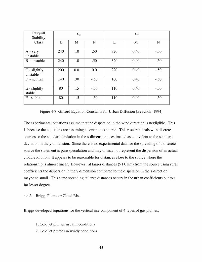
4.4.2 Pasquill Stability Classes and Experimental Dispersion Coefficients
From Lagrangian statistics it was shown that the single most important parameter for
determining dispersion of the gas cloud was the standard deviation of the wind directions, σα.
42
Estimating a meaningful parameter must consider the heating rate and wind speed. However, the
heating rate is often unknown and so it is useful to use an experimentally derived classification
scheme devised by Frank Pasquill.
The amount of turbulence in the air has a major effect upon on the rise and dispersion of a gas
plume or cloud. This turbulence has been classified into defined increments or stability classes.
The most widely used scheme is known as the Pasquill Stability Classes. It has six categories: A
- very stable σα = 25, B -unstable σα = 20, C - slightly unstable σα = 15, D - neutral σα = 10, E -
slightly stable σα = 5, and F - stable σα = 2.5. This scheme does not include very light wind
speeds on a clear night. It also does not take into effect mixed-layer height or roughness.
Increasing the roughness or decreasing the height increases the instability. Thus one way to
compensate for this is to move to the next more unstable class. See Figure 4-5 for
meteorological conditions that indicate class type.
Pasquill Stability Class Related to Wind Speed and Insolation
Where vs = stack exit velocity [m/d] and r2 = stack exit area [m2]
4.4.5 Briggs Stability Parameter
Briggs defines a stability parameter, s, also known as the restoring force that indicates the effect atmospheric turbulence has on the plume or cloud rise. It is defined as:
S = ( gTa)dθdz
[1/s2]
Equation 4-22
49
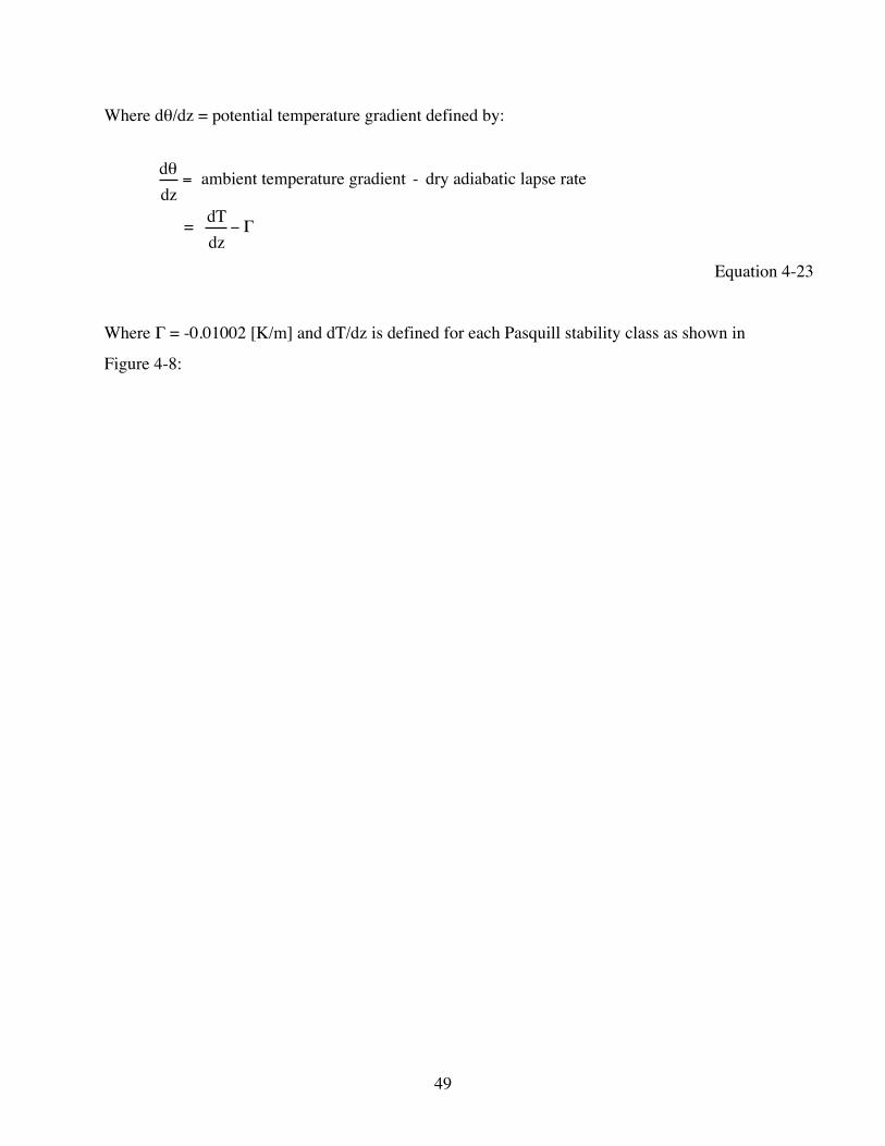
Where dθ/dz = potential temperature gradient defined by:
dθdz
= ambient temperature gradient - dry adiabatic lapse rate
= dTdz
− Γ
Equation 4-23
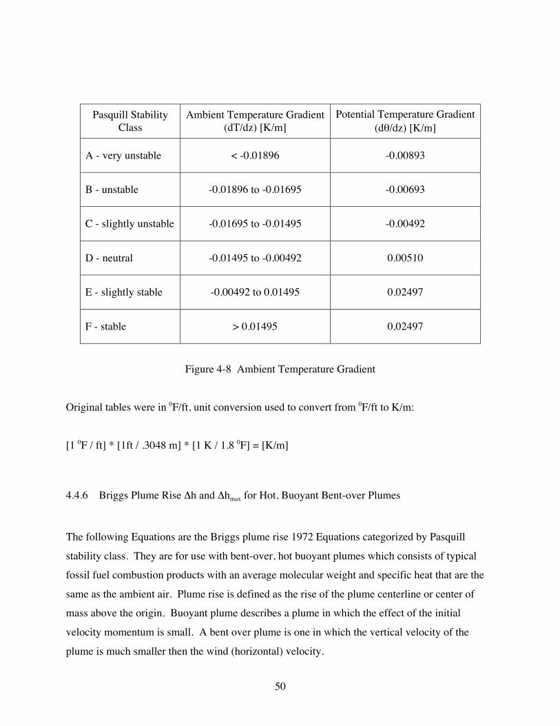
Where Γ = -0.01002 [K/m] and dT/dz is defined for each Pasquill stability class as shown in
Figure 4-8:
50
Pasquill Stability Class
Ambient Temperature Gradient (dT/dz) [K/m]
Potential Temperature Gradient (dθ/dz) [K/m]
A - very unstable < -0.01896 -0.00893
B - unstable -0.01896 to -0.01695 -0.00693
C - slightly unstable -0.01695 to -0.01495 -0.00492
D - neutral -0.01495 to -0.00492 0.00510
E - slightly stable -0.00492 to 0.01495 0.02497
F - stable > 0.01495 0.02497
Figure 4-8 Ambient Temperature Gradient
Original tables were in 0F/ft, unit conversion used to convert from 0F/ft to K/m:
4.4.6 Briggs Plume Rise Δh and Δhmax for Hot, Buoyant Bent-over Plumes
The following Equations are the Briggs plume rise 1972 Equations categorized by Pasquill
stability class. They are for use with bent-over, hot buoyant plumes which consists of typical
fossil fuel combustion products with an average molecular weight and specific heat that are the
same as the ambient air. Plume rise is defined as the rise of the plume centerline or center of
mass above the origin. Buoyant plume describes a plume in which the effect of the initial
velocity momentum is small. A bent over plume is one in which the vertical velocity of the
plume is much smaller then the wind (horizontal) velocity.
51
The basic theory makes the following assumptions:
1. Buoyancy is conserved. I.e., motion is considered adiabatic - no heat loss:
dθpdt
= 0
Equation 4-24
Where θp=local potential temperature in plume at h = height [m], t = time [s]
2. Pressure forces are small and have little effect on plume motion:
d vp→
dt=gΤ
# θ κ→
Equation 4-25
Where v→
p = local velocity of gas in plume [m/s], g = gravitational constant [9.8 m/s2], T
= temperature ambient air [K], θ' = θp - temperature of air at height, h [K], k→
= unit
vector in vertical direction
3. Molecular viscosity is negligible due to plume Reynolds number being high thus local
density changes are neglected:
∇⋅ρp v→
p = 0
Equation 4-26
Where ∇ = gradient operator = x∧ δ
δx+ y
∧ δ
δy+ z
∧ δ
δz, ρp = local gas density [g/m3]
52
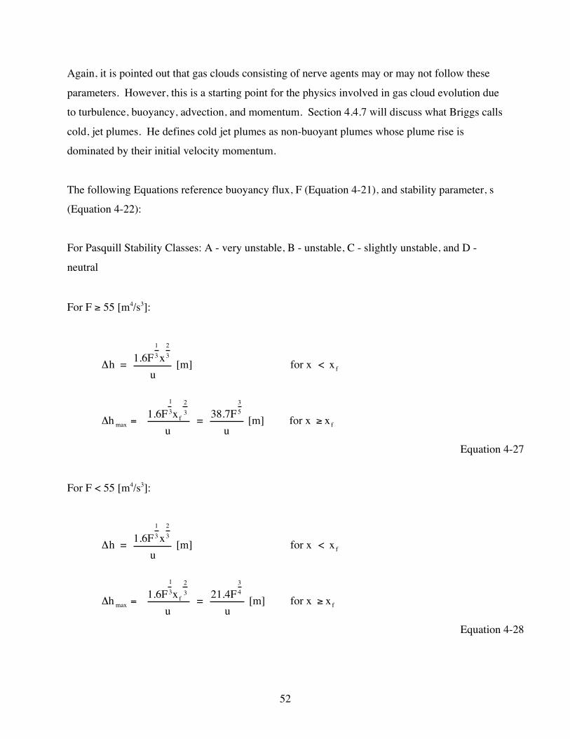
Again, it is pointed out that gas clouds consisting of nerve agents may or may not follow these
parameters. However, this is a starting point for the physics involved in gas cloud evolution due
to turbulence, buoyancy, advection, and momentum. Section 4.4.7 will discuss what Briggs calls
cold, jet plumes. He defines cold jet plumes as non-buoyant plumes whose plume rise is
dominated by their initial velocity momentum.
The following Equations reference buoyancy flux, F (Equation 4-21), and stability parameter, s
(Equation 4-22):
For Pasquill Stability Classes: A - very unstable, B - unstable, C - slightly unstable, and D -
neutral
For F ≥ 55 [m4/s3]:
Δh = 1.6F13 x
23
u [m] for x < xf
Δh max = 1.6F13xf
23
u = 38.7F
35
u [m] for x ≥ xf
Equation 4-27
For F < 55 [m4/s3]:
Δh = 1.6F13 x
23
u [m] for x < xf
Δh max = 1.6F13xf
23
u = 21.4F
34
u [m] for x ≥ xf
Equation 4-28
53
For Pasquill Stability Classes: E - slightly stable and F - stable
For 1.8 u s-1/2 ≥ xf:
Δh = 1.6F13 x
23
u [m] for x < xf
Δh max = 1.6F
13xf
23
u =
38.7F35
u [m] for x ≥ xf and F ≥ 55 [m 4/s3 ]
Δhmax = 1.6F
13xf
23
u =
21.4F34
u [m] for x ≥ xf and F < 55 [m4 /s3 ]
Equation 4-29
54
For 1.8 u s-1/2 < xf:
Δh = 1.6F
13 x
23
u [m] for x <
1.84u
s
Δhmax = 2.4(Fus)
13 [m] for x ≥
1.84u
s
Equation 4-30
Where Δh = initial plume rise [m], Δhmax = max plume rise [m], x = downwind distance from
source [m], x* = distance to final stage [m], xf = distance to max plume rise [m] = 3.5x*, 3.5x* =
119F4/5 for F ≥ 55 [m4/s3], 3.5x* = 49F5/8 for F < 55 [m4/s3], u = wind velocity [m/s], F =
buoyancy parameter [m4/s3], and s = stability parameter [1/s2]
4.4.7 Briggs Plume Rise Δh and Δhmax for Cold, Jet Bent-over Plumes Briggs defines plume rise for cold, bent-over jet plumes according to Pasquill stability class
using the same principles discussed under hot, bent-over buoyant plumes. The major difference
being jet plumes are dominated by initial velocity momentum. Unheated plumes composed
mostly of air fit into this category.
Briggs defines a momentum flux parameter to account for the velocity momentum
(mass*velocity):
Fm = momentumπρa
=(ρsVs )vs
πρa
=(ρsπr2 vs )vs
πρa
= (ρs r
2 v2s )
ρa
Using the Boussinesq Approximation becomes
= (Ta
Ts
)r2 v2s [m4 /s2 ]
Equation 4-31
55
Where Ta = ambient air temperature [K], Ts = plume gas temperature [K], r = stack exit radius [m], vs = stack exit velocity [m/s], Vs = stack gas flow [m3/s], ρs = stack gas density [g/m3], ρa = ambient air density [g/m3]
Briggs Equations for bent-over, cold jet plume rise with Pasquill stability classes A, B, C, and D
(unstable to neutral) are defined as:
Δh = 2.3(Fm x)
13
u23
Δhmax = 6rvs
u
Equation 4-32
Where Fm = momentum flux parameter [m4/s2], x = downwind distance [m], u = wind speed
[m/s], r = stack radius [m], vs = stack exit velocity [m/s]
Briggs Equations for bent-over, cold jet plume rise with Pasquill stability classes E and F (stable
to very stable) are defined as:
Δhmax = 1.5Fm
13
u13s
16
[m]
Equation 4-33
Where Briggs has not defined Δh in the literature for this type of plume.
4.4.8 Briggs Plume Rise Δh and Δhmax for Vertical Plumes
Vertical plumes arise when the horizontal wind velocity is negligible. Briggs (1969) defines the
maximum plume rise for Pasquill class E and F, vertical, hot buoyant plumes as:
56
Δhmax =5.0F
14
s38
[m]
Equation 4-34
Briggs (1969) defines the maximum plume rise for Pasquill class E and F, vertical, cold jet
plumes as:
Δhmax =4.0Fm
14
s14
[m]
Equation 4-35
4.5 Determining Cloud Dispersion and Rise Parameters
Sections 4.1 – 4.4 established the theory on which the Gaussian model is based on.
Make_blob.cc is a program written in C++ based on the experimental data and equations
presented by Pasquill and Briggs in the preceding sections. Pasquill discusses how to determine
the standard deviation to be used in the Gaussian equation. Briggs examines how to determine
the rise associated with a cloud based on initial momentum and temperature. Both the standard
deviation and rise are associated with Pasquill classes. These Pasquill classes incorporate the
effect of turbulence on the cloud. Make_blob.cc reads in a data file that describes the
environmental conditions (i.e., wind speed, insolation, rate of release, cloud cover, starting x, y, z
coordinates, see Appendix A for a complete listing of input parameters). It then uses this
information to determine the Pasquill class, standard deviation of the Gaussian PDF, and the rise
(based on the Brigg’s bent, over hot plume equations). Make_blob.cc then outputs a Gaussian
PDF and final x, y, z coordinates according to the Pasquill and Brigg’s equations. For
completeness, cold jet plumes and hot, buoyant plumes in calm conditions are discussed but are
not included in make_blob.cc.
57
5 Limitations of Gaussian Models
This section discusses the assumptions and constraints involved with using the Gaussian
dispersion equations for modeling gaseous clouds from a single point source in flat terrain.
5.1 Assumptions and Constraints
The nature of modeling gas clouds involves certain assumptions about the conditions that effect
the evolution of the cloud. These constraints are used to limit the number of variables involved
and hence simplify the complexity of the problem. The drawback to these assumptions is that
the prediction by the simulation will differ from the real cloud evolution. The addition of more
variables may produce a better prediction but at the cost of computational time. Even if every
variable could be included there would still be an inherent randomness or chaotic nature that the
simulation would not be able to predict.
The Gaussian dispersion equations assume the following:
1. The wind speed and direction are constant throughout the evolution.
2. Atmospheric turbulence does not change throughout the evolution.
3. The mass of the plume is conserved.
4. Only crosswind and vertical dispersion occurs. This research assumes the downwind
dispersion is the same as the crosswind dispersion.
5. The cloud PDF expands with a Gaussian distribution. The evolution of a cloud could
have other distributions depending on the initial blast conditions, wind changes,
turbulence factors, etc…
6. Using either urban dispersion coefficients or rural dispersion coefficients
accommodates for terrain conditions. The basic Gaussian dispersion equation was not
meant to handle coastal terrain, valleys, mountains, etc…
58
In short, the Gaussian models assume an ideal steady state of constant meteorological conditions over long distances, idealized plume geometry, uniform flat terrain, complete conservation of mass, and exact Gaussian distribution. Such ideal conditions rarely occur. [Beychok]
It is important to mention that these assumptions make the basic Gaussian model a simple tool
that can assist the user but does not provide exact answers. The model is a start but can be
improved upon. Some of these improvements are discussed in the section titled: Conclusion and
Improvements.
59
6 Rendering
6.1 Raytracing
For a more complete explanation on raytracing the reader can refer to almost any text on
computer graphics and rendering.
Raytracing uses the principles of geometric optics to traverse the path propagated by light beams
(rays) from the sensor to the source. The sensor will have some plane of view to reduce the
number of rays that need to be cast or sent out into the scene. The plane of view can be broken
up into a rectangular grid. See Figure 6-1.
Figure 6-1 Simple Raytracing Process [Fusner, 1999]
Any two points in space define a vector. That vector must go through the plane of view in order
to be used. The vector is then extended out to the scene, i.e. an AutoCAD drawing, to determine
if it intersects an object. If no intersection occurs then a default radiance is assigned. When an
intersection occurs then a ray is sent to the illumination sources to determine the radiance falling
on that point. Other optical properties that may be calculated include single or multiple
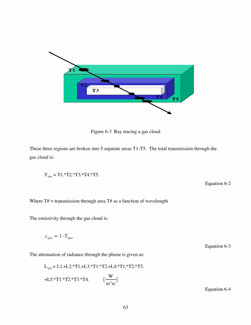
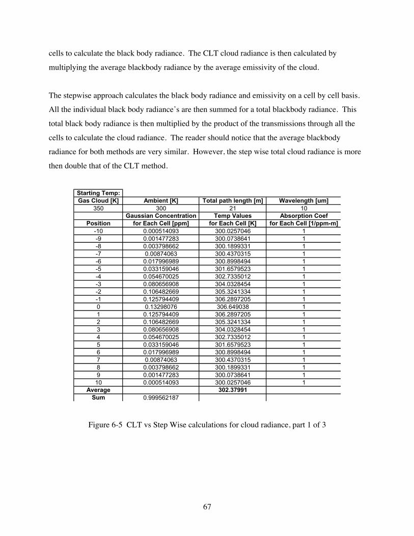
Figure 6-5 CLT vs Step Wise calculations for cloud radiance, part 1 of 3
68
Wavelength [um]10 Base 10
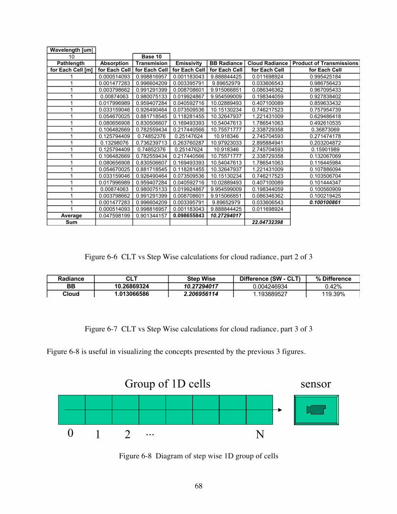
Pathlength Absorption Transmision Emissivity BB Radiance Cloud Radiance Product of Transmissionsfor Each Cell [m] for Each Cell for Each Cell for Each Cell for Each Cell for Each Cell for Each Cell
Figure 6-7 CLT vs Step Wise calculations for cloud radiance, part 3 of 3
Figure 6-8 is useful in visualizing the concepts presented by the previous 3 figures.
0 N
sensorGroup of 1D cells
1 2 ...
Figure 6-8 Diagram of step wise 1D group of cells
69
Once the ray leaves the cloud DIRSIG continues with ray tracing through the rest of the scene.
6.3 Noise Artifacts
Noise is defined as an unexpected variation in the signal received at the output. In remote
sensing the sources of noise are broken into three major categories: scene, sensor, and
processing, see Figure 6-9.
Electrical
Scene
Noise factors and variability degrading information content
Surface Goniometric Atmospheric
-Within classvariation
-Backgroundvariations
-Mixedpixels
-Adjacentreflections
-Surfaceslope& aspect
-Obscuringobjects
-Illuminationangle
-View Angle
-Polarization
-Specularreflection
-Absorption
-Scattering
-Path radiance
-Sky radiance
-Variability
-Cloud effects
Sensor
Mechanical System
-Thermal
-Shot
-Quantization
-Crosstalk
-Temperatureinduced
-Electrical transfer function
-Blur
-Vibration
-Multi-sensordistortion
-Optical transferfunction
-Calibrationuncertainty
-Scatteringwithin optics
-Scanning &Sampling effects
Processing
Computational Analyst
-Resampling
-Misregistration
-Compression,coding
-Round-off
-Training setsize
-Training seterrors
-Errors of assumption
Figure 6-9 Noise and information degrading effects in a remote sensing system [Kerekes, 1987]
The remote sensing of gas clouds using multi-spectral simulations would be most effected by
spectrally correlated noise. The output digital count is a function of the incident radiance onto the
detector. Ideally each detector would output the same digital count for the same incident
radiance both spatially and spectrally. Any shift in the system spectral response after ground
spectral calibration will cause a shift in the band edges.
70
If these spectral changes go unnoticed, they can introduce radiometric calibration errors, atmospheric correction errors, and misinterpretation of spectral signatures. The relative importance of these changes will depend a great deal on the calibration techniques used and on where the spectral shift occurs relative to spectral structure in the target or the atmosphere (i.e., a very small change at the edge of an atmospheric window could have a major impact, whereas a large change in the middle of window or in a spectral region where the target and backgrounds were slowly varying would have limited impact.) [Schott, 1997]
The spectral signature of the gas can be altered by spectrally correlated noise. Currently,
DIRSIG does not include spectrally correlated noise in the final image. Therefore, spectrally
correlated noise should be added in post processing to the final output image in order to
investigate the effects on detection of the gas cloud. Unfortunately, spectrally correlated noise is
detector dependent. One way to characterize the spectrally correlated noise would be to use dark
current readings for each band prior to acquiring an image. The dark current image is the signal
generated by the system when there is no incident radiation, thus the dark image can be used to
characterize the spatial and spectral noise of the system.
71
7 Validation
Validation of the gas model requires experimental data. Unfortunately, there is none available at
this time. Releases of toxic agents are extremely dangerous and it is for this reason they are not
done. The availability of truth data would be a great help in incorporating improvements and
investigating the evolution of a cloud in a real environment. An alternative to releasing toxic
agents would be to release a benign gas with a similar molecular weight as the toxic gas to be
studied. Appendix E briefly describes a design experiment outlining a procedure for such a
release. The validation of this research involved verifying offline that DIRSIG was computing
the correct values given the equations used. This included sanity checks on mass, volume, total
concentration, and spatial sampling as a function of time. Online (inside DIRSIG),
phenomenology such as diffusion, reduced concentrations and temperature were investigated.
Finally, offline (outside DIRSIG) calculations of integrated radiance, dilution, transmission,
column density, and temperature were calculated and compared to the DIRSIG calculations.
7.1 Voxel file validation
Voxel files are created by the C++ program, make_blob.cc, and altered to include fBm fields
generated by the IDL program fbm.pro. Voxel files are used by the DIRSIG gas model and
contain information describing the 3D Gaussian PDF. It has the following format:
Line 1: x, y, z insertion points; x, y calculated using wind speed and direction and z
calculated using Brigg’s buoyancy equation
Line 2: x, y, z Gaussian PDF size; dimensions of Gaussian cube
Line 3: scale - how long each side of a voxel is in gdb units
Line 4 – to EOF: 3D Gaussian PDF in 1D format, where Gauss(x,y,z) =
z*x_size*y_size + y*y_size + x; i.e. The value for 3D Gauss(3,5,9) if x_size= y_size =
z_size = 10 would be found at 900 + 50 + 3 = 953 + 3 = line 956 of the voxel file.
72
The information in these files was checked offline to ensure the total concentration (mass /
volume) remains constant throughout a time evolution. This assumes no mass losses due to
downwash, dry removal, vegetation, etcetera. Since the mass is conserved the total
concentration is a constant mass * inverse volume (represented by the Gaussian PDF). Based on
the probability of observations for a normal distribution and using three standard deviations the
concentration of a 1D Gaussian with mass of 1 gram is approximately: 1 [g] * 0.9974 [1/m] =
0.9974 [g/m]. In 3D, the total concentration with mass of 1 gram becomes: 1 [g] * (0.9974 [m])3
= 0.9922 [g/m3]. The total inverse volume was calculated by summing the individual Gaussian
PDF values. The total inverse volume was consistently, out to about four decimal place, around
the expected 0.9922 [1/m3]. Thus, the concentration is within 0.1 % of the expected value.
7.2 DIRSIG sampling
It is important to determine if DIRSIG samples the voxel file correctly. The sampling size can
be determined by knowing the focal length, height above the target, array size, and the scene
units. Once the sample size was determined it was then compared to the known voxel
dimensions to ensure that the cloud was the proper size. The sample size was determined using
similar triangles and the following calculations:
Given: scene units = inches, default x, y array size, A = 0.974 [in], image size = 128x128
[pixels], focal length, f = 0.787 [in], height above target, H = 10500 [in], cloud size =
787x787x787 [in].
73
Figure 7-1 Geometric construction for sampling transformation
G2
[in] = H [in]*
A2
[in]
f [in]
= 10500 [in] * 0.487 [in]
0.787 [in] = 6497.5 [in]
Equation 7-1
Detector resolution [in / pix] =
G [in]2
image size [pix]2
= 6497.5 [in]
64 [pix]= 101.5 [
inpix
]
Equation 7-2
74
Pixels needed to represent cloud [pix] = Size of cloud [in]
Detector resolution [in
pix]
= 787 [in]
101.5 [ inpix
]= 7.75 [pix]
Equation 7-3
The number of pixels used by DIRSIG was 8, which is acceptable since discrete sampling
methods are used.
7.3 DIRSIG debug images
DIRSIG produces debug images that allow the user to examine various DIRSIG outputs. These
include: cloud dilution [1/m3], cloud temperature [K], cloud column density [ppm-m], cloud
transmission, and cloud radiance [W/m2Ω]. It is important that these images contain accurate
data based on the equations used. The DIRSIG data was subjected to a comparison offline to
validate that the answers were accurate.
Cloud dilution represents the integrated 3D Gaussian values through the cloud at a specified
angle. This was tested by constructing a voxel file of known dimensions (20x20x20) with each
element set to one. The dilution was calculated offline by integrating through the voxel files and
compared to the DIRSIG output. Various sampling scales were used with a nadir look angle. It
is important to note that cloud dilution is not a function of area but a function of path length
through the cloud. Thus, the dilution should be the same for each pixel regardless of the scale as
long as the size of the cloud has not changed. DIRSIG output was with in 5-10% of the correct
dilution of 20. The error can be attributed to discrete sampling of the cloud and varies with
sampling scale and cloud size. For example, a one-voxel error in the above scenario produces a
5% error. However, that same one voxel error for a voxel file of dimensions 100x100x100
would show only a 1% error. Thus, an error in precision will have a much larger impact for gas
clouds that are just starting to evolve.
75
Cloud temperature calculates the cloud temperature distribution based on the cloud dilution and
the initial cloud temperature, see Equation 6-9. These values were calculated offline using the
cloud dilution and Equation 6-9 and compared to the DIRSIG output. The DIRISIG calculation
was with in 5-10% of the correct temperature. Again, these errors arise from errors in the
dilution calculations due to discrete sampling.
Cloud column density is the concentration over a given length through the gas based on the cloud
dilution, total mass, molecular weight, ideal volume of the gas @ STP, and the total path through
the gas cloud (see Equation 6-8). The molecular weight, total mass, and ideal volume are all
constants throughout the time evolution. Differences in column density are dependent on the
cloud dilution and the look angle. The look angle will determine the path length through the
cloud by indicating the vector in and out points for the cloud data. The distance through the
Equation 7-4 Where Xout, Yout, Zout are coordinates [m] of the vector leaving the cloud and Xin, Yin, Zin are coordinates [m] of the vector entering the cloud.
As expected, using Equation 6-8 the DIRSIG column density was within 5-10% of the calculated
column density. Again, the error is attributed to scaling and discrete sampling and will fluctuate
based on scale and cloud size.
Cloud transmission is based on the absorption, see Equation 2-13. The absorption is a function
of the absorption coefficient, the concentration, and the path length through the cloud, see
Equation 2-14. These values were calculated offline using Equation 2-13 and Equation 2-14 and
compared to the DIRSIG output. The DIRSIG cloud transmission was within 5-10% of the
calculated cloud transmission. Again, the error is attributed to scaling and discrete sampling and
will fluctuate based on scale and cloud size.
76
Cloud radiance [w/m2Ω] is based on the emissivity, see Equation 6-3, through the gas cloud
times the blackbody radiance, see Equation 2-23. The total radiance was calculated offline and
compared to the DIRSIG output. The DIRSIG cloud radiance was within 5-10% of the
calculated cloud radiance. The error is attributed to scaling and discrete sampling and will
fluctuate based on scale and cloud size.
To summarize, the primary difference between offline calculated values and DIRSIG stems from
a discrete sampling issue. The error in precision will have a more profound effect on small gas
clouds. It is speculated that the sampling error is introduced because the 3D-DDA does not
identify all voxels pierced by the ray. A new sampling algorithm that includes all voxels pierced
by a ray may reduce or eliminate this sampling issue, see Heckbert (1994).
77
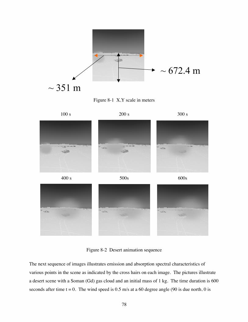
8 DIRSIG synthetic scenes
The following section includes images to qualitatively investigate the cloud model.
8.1 Examples
The following animation was rendered with DIRSIG using the theory presented in the previous
sections. The pictures illustrate a desert scene with a Soman (Gd) gas cloud and an initial mass
of 1 kg. The time duration is 100 – 600 seconds after time t = 0 in 100 second increments. The
wind speed is 0.5 m/s at a 60 degree angle (90 is due north, 0 is east). The Pasquill stability class
is D (neutral) with rural coefficients. The initial gas temperature is 350 K and the spectral bands
are integrated over 900 – 1100 cm-1, which is the peak absorption range for Soman gas. Gain
and Bias are the same for each image for comparison purposes. It illustrates some interesting
phenomenology. The desert sand is very warm due to thermal loading from the sun. The gas
cloud is actually cooler then the background. This is why the cloud is darker than the sand.
However, compared to the horizon the gas cloud is still warmer than the air. It also illustrates the
diffusion of the cloud over time.
78
~ 672.4 m
~ 351 m
Figure 8-1 X,Y scale in meters
100 s 200 s 300 s
400 s 500s 600s
Figure 8-2 Desert animation sequence
The next sequence of images illustrates emission and absorption spectral characteristics of
various points in the scene as indicated by the cross hairs on each image. The pictures illustrate
a desert scene with a Soman (Gd) gas cloud and an initial mass of 1 kg. The time duration is 600
seconds after time t = 0. The wind speed is 0.5 m/s at a 60 degree angle (90 is due north, 0 is
79
east). The Pasquill stability class is D (neutral) with rural coefficients. The initial gas
temperature is 350 K. Same scale as previous images.
Tit le:a_emit.psCreator:gnuplot 3.5 (pre 3.6) patchlevel beta 347Prev iew:This EPS picture was not savedwith a preview included in it.Comment:This EPS picture will print to aPostScript printer, but not toother types of printers.
Figure 8-3 Point A, cloud emission with background interaction
Tit le:b_absorb.psCreator:gnuplot 3.5 (pre 3.6) patchlevel beta 347Prev iew:This EPS picture was not savedwith a preview included in it.Comment:This EPS picture will print to aPostScript printer, but not toother types of printers.
Figure 8-4 Point B, Gas cloud absorbing against atmosphere
80
Tit le:cld_bkgd_absorb.epsCreator:gnuplot 3.5 (pre 3.6) patchlevel beta 347Prev iew:This EPS picture was not savedwith a preview included in it.Comment:This EPS picture will print to aPostScript printer, but not toother types of printers.
Figure 8-5 Point B2, Gas cloud emission against background
Tit le:b_emit.psCreator:gnuplot 3.5 (pre 3.6) patchlevel beta 347Prev iew:This EPS picture was not savedwith a preview included in it.Comment:This EPS picture will print to aPostScript printer, but not toother types of printers.
Figure 8-6 Point C, high cloud emission
81
Tit le:c_bkgd.psCreator:gnuplot 3.5 (pre 3.6) patchlevel beta 347Prev iew:This EPS picture was not savedwith a preview included in it.Comment:This EPS picture will print to aPostScript printer, but not toother types of printers.
Figure 8-7 Point D, background spectra
Tit le:d_atm.psCreator:gnuplot 3.5 (pre 3.6) patchlevel beta 347Prev iew:This EPS picture was not savedwith a preview included in it.Comment:This EPS picture will print to aPostScript printer, but not toother types of printers.
Figure 8-8 Point E, atmospheric spectra
82
The next pictures are of a scene with a slant angle of 5 degrees at 1500 seconds after release.
The initial mass was 200 kg, initial temperature was 350 K and the distance from the cloud to the
sensor is approximately 1.5 km. It demonstrates the different absorption peaks at the three wave
numbers. It also demonstrates that Soman gas has a higher absorbence in band 1020 [cm-1] than
in bands 900 and 1100 [cm-1] with band 900 [cm-1] having the least absorbence of the three. This
agrees with the gas absorption data supplied by the Army’s Aberdeen Proving Grounds.
~ 1256.3 m
~ 522.6 m
Figure 8-9 X,Y image scale in meters
900 cm-1 1020 cm-1 1100 cm-1
Figure 8-10 Desert release, 1500 seconds
The next sequence of images illustrate an urban scene with a Soman (Gd) gas cloud and an initial
mass of 0.5 kg. The time duration is 25 - 500 seconds in 100 second increments after time t > 0.
The wind speed is 0.5 m/s at an 80 degree angle (90 is due north, 0 is east). The Pasquill
stability class is A (unstable) with urban coefficients. The initial gas temperature is 350 K and
83
the spectral bands are integrated over 990 - 1100 [cm-1] in 10 [cm-1] increments. Gain and Bias
are the same for each image for comparison purposes.
~ 186 m ~ 407.1 m
Figure 8-11 X,Y scale in meters
25 s 125 s 225 s
325 s 425 s 500 s
Figure 8-12 Urban animation sequence
84
The animations shown above demonstrate a decrease in concentration and emissivity as the size
of the gas cloud increases. This follows the theoretical expectations.
The next set of images demonstrates the spectral “finger print” of the cloud as a function of
transmission through the cloud. The scene shows a 1 Kg release at 575 seconds after t = 0. The
Pasquill stability class is D (neutral) with rural coefficients. The initial gas temperature is 350 K
and the spectral range is 800 – 1050 [cm-1] at 0.25 [cm-1] increments (FASCODE). The
background is a black body radiator with temperature set to 0 K. For these scenes the
atmosphere between the target and sensor has been removed. Same image scale as Figure 8-1.
0.00085
0.0009
0.00095
0.001
0.00105
0.0011
0.00115
800 850 900 950 1000 1050
Radiance [W / (m^2 sr)]
Wavenumber [cm^-1]
Soman (GD) Gas Cloud Center Radiance
Figure 8-13 Spectral "finger print" radiance for center of GD gas cloud
85
0.00055
0.0006
0.00065
0.0007
0.00075
0.0008
0.00085
0.0009
0.00095
0.001
0.00105
800 850 900 950 1000 1050
Radiance [W / (m^2 sr)]
Wavenumber [cm^-1]
Soman (GD) Gas Cloud Edge Radiance
Figure 8-14 Spectral "finger print" radiance for edge of GD gas cloud
Blob.dat is a text file containing three data lines describing environmental and other pertinent
parameters. The data lines start with the letters d(ata), p(osition), or b(uoyancy). Make_blob.cc
reads the data in blob.dat to create the Gaussian blobs. The following illustration is an example
of a blob.dat file:
data file for make_blob.cc, # means a comment follows: #data parameters # wind [m/s], cloud [0-none, 1-all cloud], insolation [w/m^2], # am_pm [0-am, 1-pm], time [s], rur_urb [0-rur, 1-urb], # Pclass [A-F,G,H,I,Z - let model choose based on wind & insolation], # time increment [divisions from time =0 to time end] #position parameters #start_x, start_y, start_z, theta [degrees 0-360], scale [dist/voxel], units #[F = feet, M = meters, C = centimeters, I = inches], vxl_scale #buoyancy parameters #exit_vel [m/s], exit_radius [m], temp_air [K], temp_gas [K] d 0.5 0 600 1 0 600 1 Z 1 p 38292 33760 3000 60 1 I 2.0 b 1.0 .2 273 300
94
where 1. wind = wind speed in meters per second
2. cloud = percentage of cloud cover, range is from 0 - 1. 0 is no clouds, 1 is 100%
3. insolation = amount of irradiance in watts per meter squared the gas encounters
4. am_pm = night or day, 0 - day, 1 - night
5. start_time = start time of vxl creation in seconds
8. Pclass - Pasquill class, A-F, G = average of A + B, H = Average of B + C, I = Average
of C + D. set equal to Z to let make_blob calculate based on wind speed, insolation,
and day/night. Must be in CAPS.
9. time increment = number of increments to break time up into. I.e. if time was set to 100
seconds and you wanted a vxl_file every 10 seconds then the increment would be 10.
10. start_x, start_y, start_z - x, y, z starting coordinates
11. theta = wind direction in degrees, 0 = due east, 90 = due north.
12. scale = set to 1
13. units = gdb units used by DIRSIG: C - cm, M - m, I - inches, F - feet, must
be in CAPS.
14. vxl_scale = sampling scale to use when creating vxl_file. I.e., 0.5 = 2 pixels for every one
GDB_UNIT, 1 = 1 pixel for every GDB_UNIT, 2 = 0.5 pixels for every GDB_UNIT,
etc...smaller then one is oversampling, greater then one is undersampling. Allows the creation of
very large Gaussian blobs through down sampling or very small Gaussian blobs through over
sampling.
15. exit_vel = rate of gas from dissemination unit in meters per second
16. exit_radius = diameter of dissemination unit, set small for a point source release, set larger
for a larger object release
17. temp_air = ambient air temperature in Kelvin at the time of release
18. temp_gas = temperature of gas in Kelvin at release
To create an animation change start time and end time to cover the time window
95
of interest. Set time_increment to break up range into divisions. Set all other parameters. Run
make_blob executable. I.e., to make an animation from 25 seconds to 225 seconds after release
at 10 second intervals set start time = 15 , end time = 225 and time_inc = 21. This will produce
blob??.vxl. The question marks will be the time in seconds after release. Each time increment
will have its own blob file. ALL PARAMETERS MUST BE SET!!!. Make_blob.cc does not
provide error checking so it may fail or produce erroneous results if all parameters are not set.
10.2 FBm.pro
FBm.pro is an interactive display language (IDL) program used to create texture maps for each
voxel file created by make_blob.cc. The source code requires the language IDL to run. Fbm.pro
requires the modules: gaus_amp.pro, gaus_phase.pro, and gaus_randist.pro. Gaus_amp.pro
generates the amplitudes required for fractional Brownian motion. Gaus_phase.pro generates the
Hermetian phase distribution. Gaus_randist.pro generates a 3D random Gaussian distribution
with even symmetry about its center. The program is based on the theory in section 3.5.1.
To run fBm.pro move all the voxel files into the same directory as fbm.pro. Run fbm.pro in IDL
by typing:
>idl
idl>.run fbm.pro
idl>fbm
The output will be files called fbm_blob???.vxl. The question marks are the time in seconds
after the initial release.
The parameter B can be changed in the file: gaus_amp.pro line 28.
It is currently set to 1.50. This will change the weighting of frequencies included in the 1 / f^B
relationship. Decreasing this number will add more noise.
The variance can be changed on line 12 of fbm.pro. This controls the apparent
96
randomness around the mean.
The fbm voxel file has the following format:
Line 1: x, y, z insertion points; x, y calculated using wind speed and direction and z
calculated using Brigg’s buoyancy equation
Line 2: x, y, z Gaussian PDF size; dimensions of Gaussian cube
Line 3: scale - how long each side of a voxel is in gdb units
Line 4 – to EOF: 3D Gaussian fBm PDF in 1D format, where Gauss(x,y,z) =
z*x_size*y_size + y*y_size + x; i.e. The value for 3D Gauss(3,5,9) if x_size= y_size =
z_size = 10 would be found at 900 + 50 + 3 = 953 + 3 = line 956 of the voxel file.
This is the format required by DIRSIG.
97
11 Appendix B: DIRSIG Configuration File Changes
This section discusses the configuration changes (extension .cfg) needed by DIRSIG in order to
run the gas model. See Brown (1999) for a complete description of each section.
11.1 Original Configuration File Example
This section includes an example configuration file required for DIRSIG runs. It is also required
by make_adb to create the atmospheric database (extension .adb).
DIRSIG_CFG # # DIRSIG Run-Time Configuration File # PATHS { EMISSIVITY_PATH = /dirs/home/dirsig/training/desert/emissivity EXTINCTION_PATH = /dirs/home/dirsig/training/desert/extinction MAPS_PATH = /dirs/home/dirsig/training/desert/maps } # # The SCENE section describes what geometric database(s) are being # modeled, what units the GDB is in, what altitude a height of 0.0 in # the GDB translates to, where the scene is physically located, time # of day, day of year, # SCENE { GDB_FILENAME = ./desert.gdb GDB_UNITS = INCHES MATERIAL_FILENAME = ./desert.mat GROUND_ALTITUDE = 0.218 DATE = 6 24 1996 GMT_TIME = 17.50 GMT_OFFSET = 5.0 LATITUDE = 43.00 LONGITUDE = 78.00 } # # The ENVIRONMENT section describes the atmosphere and meteorological # conditions at the scene. # ENVIRONMENT { TAPE5_FILENAME = ./desert.tp5 ADB_FILENAME = ./desert_nadir.adb
98
WEATHER_FILENAME = ./desert.wth } # # The PLATFORM section describes the sensor system being used for the # simulation. This includes information such as the position of the # sensor and the geometric/spectral description of each band in the # system. # PLATFORM { POSITION { # TARGET_LOCATION = 1840.00, 1840.00, 0.0 # TARGET_LOCATION = 960.00, 1216.00, 0.0 # PLATFORM_LOCATION = 960.00, 2000.00, 794.0 TARGET_LOCATION = 41894.0, 39987.0, 3000.0 PLATFORM_LOCATION = 41894.0, 39987.0, 13500.0 AZIMUTH_ANGLE = 90.0 # ELEVATION_ANGLE = 70.0 } INSTRUMENT { NAME = Generic FTS Imager TYPE = FRAMING_ARRAY FOCAL_LENGTH = 20.00 BAND_LIST { BAND { # MINIMUM_FREQUENCY = 850.0 MINIMUM_FREQUENCY = 900.0 # MAXIMUM_FREQUENCY = 1100.0 MAXIMUM_FREQUENCY = 1100.0 DELTA_FREQUENCY = 10.0 RESPONSE_FILENAME = SPECTRAL IMAGE_FILENAME = blob_desert_nadir.img X_PIXELS = 256 Y_PIXELS = 256 } } } } # flags for optional modeling OPTIONS { ENABLE_TRUTH_IMAGES = TRUE ENABLE_MAPS = TRUE ENABLE_THERMAL_MODEL = TRUE ENABLE_PLUMES = TRUE } #
99
# The TRUTH_IMAGES section controls which debug images will be generated. # If this section does not appear, the default debug list in # $DIRSIG_HOME/lib/default.dbl is used. This section is ignored if the # ENABLE_TRUTH_IMAGES flag is set to FALSE. # TRUTH_IMAGES { IMAGE_FILENAME = blob_desert_nadir_truth.img MATERIAL_MAPS = TRUE HIT_MAPS = TRUE TEMPERATURE_MAPS = TRUE PLUME_MAPS = TRUE } # # The MAPS section describes material and texture maps applied to # various materials in the scene. This section is ignored if the # ENABLE_MAPS flag is set to FALSE. # MAPS { # override desert_wash areas with scene map MATERIAL_MAP { IMAGE_FILENAME = desert_map.pgm INSERT_POINT = 25000,75000,0 GSD = 26.6 MATERIAL_ID = 100 LUT { 0 = 8 # map desert_wash (8) to 0 128 = 9 # map dirt_road (9) to 128 255 = 10 # map desert_pavement (10) to 255 } } # Texture for sand TEXTURE_MAP { IMAGE_FILENAME = sand.pgm INSERT_POINT = 25000,75000,0 GSD = 15.0 MATERIAL_ID = 8 MINIMUM_WAVELENGTH = 0.45 MAXIMUM_WAVELENGTH = 0.52 } # Texture for dirt road TEXTURE_MAP { IMAGE_FILENAME = dirt.pgm INSERT_POINT = 25000,75000,0 GSD = 15.0 MATERIAL_ID = 9 MINIMUM_WAVELENGTH = 0.45 MAXIMUM_WAVELENGTH = 0.52 } # Texture for desert pavement TEXTURE_MAP { IMAGE_FILENAME = dp.pgm
PATHS { EMISSIVITY_PATH = ./ems EXTINCTION_PATH = ./ext MAPS_PATH = ./maps ABSORPTION_PATH = ../../abs_data } # # The SCENE section describes what geometric database(s) are being # modeled, what units the GDB is in, what altitude a height of 0.0 in # the GDB translates to, where the scene is physically located, time # of day, day of year, # SCENE { GDB_FILENAME = ./desert.gdb GDB_UNITS = INCHES MATERIAL_FILENAME = ./desert.mat GROUND_ALTITUDE = 0.218 DATE = 6 24 1996 GMT_TIME = 17.50 GMT_OFFSET = 5.0 LATITUDE = 43.00 LONGITUDE = 78.00 } # # The ENVIRONMENT section describes the atmosphere and meteorological # conditions at the scene. # ENVIRONMENT { TAPE5_FILENAME = ./desert.tp5 ADB_FILENAME = ./desert_nadir.adb WEATHER_FILENAME = ./desert.wth } # # The PLATFORM section describes the sensor system being used for the # simulation. This includes information such as the position of the # sensor and the geometric/spectral description of each band in the # system. # PLATFORM { POSITION { # TARGET_LOCATION = 1840.00, 1840.00, 0.0 # TARGET_LOCATION = 960.00, 1216.00, 0.0 # PLATFORM_LOCATION = 960.00, 2000.00, 794.0 TARGET_LOCATION = 41894.0, 39987.0, 3000.0 PLATFORM_LOCATION = 41894.0, 39987.0, 13500.0 AZIMUTH_ANGLE = 90.0 # ELEVATION_ANGLE = 70.0 } INSTRUMENT {
102
NAME = Generic FTS Imager TYPE = FRAMING_ARRAY FOCAL_LENGTH = 20.00 BAND_LIST { BAND { MINIMUM_FREQUENCY = 900.0 MAXIMUM_FREQUENCY = 1100.0 DELTA_FREQUENCY = 10.0 RESPONSE_FILENAME = SPECTRAL IMAGE_FILENAME = fbm_blob100_desert_nadir.img X_PIXELS = 128 Y_PIXELS = 128 } } } } # flags for optional modeling OPTIONS { ENABLE_TRUTH_IMAGES = TRUE ENABLE_MAPS = TRUE ENABLE_THERMAL_MODEL = TRUE ENABLE_PLUMES = TRUE } # # The TRUTH_IMAGES section controls which debug images will be generated. # If this section does not appear, the default debug list in # $DIRSIG_HOME/lib/default.dbl is used. This section is ignored if the # ENABLE_TRUTH_IMAGES flag is set to FALSE. # TRUTH_IMAGES { IMAGE_FILENAME = fbm_blob100_desert_nadir_truth.img MATERIAL_MAPS = TRUE HIT_MAPS = TRUE TEMPERATURE_MAPS = TRUE PLUME_MAPS = TRUE } # # The MAPS section describes material and texture maps applied to # various materials in the scene. This section is ignored if the # ENABLE_MAPS flag is set to FALSE. # MAPS { # override desert_wash areas with scene map MATERIAL_MAP { IMAGE_FILENAME = desert_map.pgm
by running fBm.pro. Using the above scenario this will produce 21 fbm_blob??.vxl files. The
starting coordinates found in blob.dat must be chosen from actual scene coordinates. To
determine actual scene coordinates the user must run DIRSIG for a scene, enabling HIT_MAPS
= TRUE under the TRUTH_IMAGES section. The user can then use ENVI to load the x, y, and
z hitmaps as an RGB image. The user then selects from the ENVI menus: Function
Interactive Analysis Cursor Location / Value to determine the x, y, z location of each pixel in
scene units.
The second step is to run DIRSIG using the same scene with the gas model enabled. For this
scenario the same scene would run in DIRSIG 21 times. The only difference between each run is
the fbm_blob???.vxl file pointed to by the PLUME section of the configuration file. The user
should set RESPONSE_FILENAME = IDEAL located in the BAND section of the configuration
file. This will ensure that the output image is only one band. The user should also give each
output image a different name. This can be set under the BAND section as
IMAGE_FILENAME = user_defined.img and under the TRUTH_IMAGES section as
IMAGE_FILENAME = user_defined.img in the configuration file.
The third step is to convert each image file, extension .img, to a tag image file format (extension
.tiff) image. This was done using a utility at the DIRS lab called make_displayable. Its usage is:
make_displayable –t input_file output_file gain bias. Setting the gain equal to a negative number
autoscales the output into an 8-bit range. Make_displayable was used on the first image of each
106
time sequence in autoscaling mode. This provided a gain and bias that was used on all
subsequent images in that time sequence.
The fourth step is to take the scaled tiff images and use the freeware package Image Magick to
create an animation. This is done with the following command in Image Magick:
>animate *.tiff
To create an animated GIF of the sequence use the following commands in Image Magick:
>convert –delay 20 *.tiff gas_animate.gif
C-shell scripts were used to do steps 2 and 3. It is highly suggested to the user that scripts be
created to setup and run steps 2 and 3. It will save the user a great deal of time.
107
13 Appendix D: Adding Spectral Noise in ENVI
13.1 Adding Spectral Noise Using EigenVector-Based Transforms
All systems are subject to noise. Noise will have the effect of making cloud detection more
difficult especially for lower gas cloud concentrations. Hence noise should be added to the final
DIRSIG gas cloud scenes in order create more realistic scenarios for detection algorithm testing.
The idea behind eigenvector transforms is to redefine the feature space so the correlation
between elements of a random vector (in this case spectral bands) is reduced. One of the most
common of these transforms is known as principal component analysis. The multi-spectral
information is translated and rotated to increase seperability and maximize the variance. The
new output feature is known as a principal component (PC). The number of PCs will be equal to
the number of original bands, i. The first PC1 will contain the largest percentage of total scene
variance and each succeeding component PC2, PC3,…PCi will have decreasing variance. Since
each PC is orthonormal to one another each subsequent band has no correlation with the next.
Figure 13-1 illustrates.
108
DC band 1
DC band 2 R2
R1
p( DC2 )
p( PC1 )
p( DC1 ) Figure 13-1 Increased seperability and variance due to the projection onto a rotated principle component axis [Schott, 1997]
Principal component analysis can be used in the following manner to add spectrally correlated
noise, obtained from dark current images, to multi-spectral image data:
1. Take the covariance matrix of the dark current image: A.
2. Take original multi-spectral image and calculate the covariance matrix: B.
3. Add the dark current covariance matrix and the multi-spectral covariance matrix
together: M = A + B.
4. The covariance matrices A, B, and M are used to generate 3 new corresponding
matrices A”, B”, and M” where the rows, R1, R2,…Ri are ordered eigenvectors
corresponding to the ordered eigenvalues of each covariance matrix: A, B, and M.
For convenience, the rows are arranged in order of decreasing magnitude of the
corresponding eigenvalues. Thus A” is defined such that:
A"AA"T = λ1 0 00 00 0 λi
"
#
$ $ $
%
&
' ' '
109
Equation 13-1
Where A”T = the transpose of A”, A = the covariance matrix, λi = eigenvalues of A and in addition represent the variance of the ith PC.
5. Use principal components analysis (forward transform) with matrix B” to decorrelate
the image into PCs:
PC = B"T X , where
PC = PC1
PCi
!
"
# # #
$
%
& & &
Equation 13-2
Where PC = principal component of the ith band and X = vector containing i digital counts by i spectral bands 6. Use principal components analysis (back transform) using matrix M” to obtain
original multi-spectral image plus spectrally correlated noise:
PC)(M" X 1T −=
Equation 13-3 For a more rigorous treatment of principal component analysis see Schott (1997) and Castleman
(1996).
The remote sensing software ENVI 3.0b, June23rd, 1998 copyrighted and supported by Research
Systems, Inc3. can be used to apply spectrally correlated noise.
3 http://www.rsinc.com/envi
110
13.2 Adding Spectrally Correlated Noise Using a Dark Current Image
If a corresponding dark current image is available then the following procedure can be used. The
text presented here is taken from the ENVI online help and the ENVI User’s Guide version 2.0,
July 1995 edition.
A. The first step is to create a covariance matrix of the dark current image:
The Statistics option under the Basic Tools menu allows you to generate statistical reports for
image files. The covariance option (which includes eigenvectors, the covariance matrix, and the
correlation matrix) can be calculated for multi-band images only. The statistics are calculated in
The Compute Statistics Input File dialog will appear. You will select input data files using the
standard ENVI input file dialogs.
2.Select the dark current image by clicking on the file name in the list labeled "Select Input File".
4.Once the file has been selected, click "OK" to continue.
The Compute Statistics Parameters dialog will appear. You will use the Compute Statistics
Parameters dialog to select the type of statistics to be calculated and the types of reports to be
generated.
5.Select the "Covariance" check boxes.
111
Save the statistics to an ENVI format statistics file for later use with the ENVI function Principal
Components . The default file extension for statistics files is .sta.
6.Click "OK" to start the statistics calculations.
A small window appears showing the percent of processing complete as a slider from 0 to 100%.
The statistics file will contain the covariance and correlation matrices along with the
eigenvectors for each band.
B: Repeat A with multi-spectral image file:
C: Add covariance of the dark noise to covariance of the multi-spectral image. Add eigenvectors of the dark noise to the eigenvectors of the multi-spectral image:
To view statistics previously saved by the "Compute Statistics" function (as .sta files) or other
functions that create statistics files (e.g., "Principal Components").
2.When the standard ENVI file input dialog appears, select a valid statistics file.
3.Select File > Save Text to ASCII.
4.Outside of ENVI, I.e., in EXCEL, add the dark noise covariance matrix to the multi-spectral
covariance matrix. Repeat for the eigenvectors. Save the new file.
D: Decorrelate multi-spectral image using principal components analysis:
PC Rotation from Existing Stats
112
If you have already calculated covariance and eigenvalue statistics for your data, you may use
them as input into the PC Rotation. You may use any statistics file in the PC rotation that
contains covariance and eigen statistics for the same number of bands as your input data.
1.Select Transforms > Principal Components > Forward PC Rotation > PC Rotation from
Existing Stats.
2.When the standard ENVI file selection and subsetting dialogs appear, select and subset your
input file using the standard ENVI file selection procedures.
Another file selection dialog will appear, which lists all of the existing statistics file (with a
default file extension of .sta by default) in the current input data directory.
3.Select the statistics file with standard ENVI file selection procedures.
4.Select "File" or "Memory" output.
If "File" output is selected, enter a filename in the "Enter Output Filename" text box or use the
"Choose" button to select a filename.
5.Select the desired type from the "Output Data Type" pulldown menu to control the data type of
the output file.
6.Click "OK" to perform the forward PC rotation.
When ENVI has finished processing, it will load the PC bands into the Available Bands List
where they may be displayed, and the PC EigenValues plot window will appear.
E: Recorrelate, decorrelated multi-spectral image using the covariance and eigenvectors
from part C:
113
To transform principal component images back into their original data space:
1.Select Transforms > Principal Components > Inverse PC Rotation.
2.When the standard ENVI file selection and subsetting dialogs appear, select and subset your
input file using the standard ENVI file selection procedures.
Another file selection dialog will appear, which lists all of the existing statistics file (with a
default file extension of .sta by default) in the current input data directory.
3.Select the part C statistics file using standard ENVI file selection procedures.
Note: The statistics file must already exist prior to selecting the inverse PC rotation.
4.Select "File" or "Memory" output.
If "File" output is selected, enter a filename in the "Enter Output Filename" text box or use the
"Choose" button to select a filename.
5.Select the desired type from the "Output Data Type" pulldown menu to control the data type of
the output file.
6.Click "OK" to perform the inverse transform.
7.The output will be a multi-spectral image with spectrally correlated noise.
When ENVI has finished processing, it will load the bands into the Available Bands List where
they may be displayed using standard gray-scale or RGB color composite methods.
114
13.3 Adding Spectrally Correlated Noise Without a Dark Current Image
This section discusses a way in ENVI to estimate the spectral noise statistics when a dark current image is not available. This method uses the minimum noise fraction transform (MNF). See Green (1988) and Boardman (1994) for additional information. 1.Select Transforms > MNF Rotation > Forward MNF > Estimate Noise Statistics From Data. Use this option to estimate noise when you have no dark current image for your data, as is usually the case. ENVI assumes that each pixel contains both signal and noise, and that adjacent pixels will contain the same signal, but different noise. A "shift difference" is performed on the data by differencing adjacent pixels to the right and above each pixel and averaging the results to obtain the "noise" value to assign to the pixel being processed. The best noise estimate is gathered using the shift-difference statistics from a homogeneous area rather than from the whole image. ENVI will allow you to select the subset for statistics extraction. 2.When the standard ENVI file selection and subsetting dialogs appear, select and subset your input file using the standard ENVI file selection procedures. 3.When the Forward MNF Transform Parameters dialog appears, enter a filename for the noise statistics in the text box labeled "Enter Output Noise Stats Filename [.sta]." To select a homogeneous area for calculating the noise statistics, use the "Spatial Subset" button to use ENVI's standard spatial subset procedures to either manually enter a subset or to graphically indicate the area for statistics extraction. 4.Enter an output file for the MNF statistics in the text box labeled "Enter Output MNF Stats Filename [.sta]." Caution: Be sure that the MNF and noise statistics files have different names. 5.Select "File" or "Memory" output. If "File" output is selected, enter a filename in the "Enter Output Filename" text box or use the "Choose" button to select a filename. 6.Click "OK" to start the processing. 7.Use the covariance and eigenvectors from the noise statistics file as the dark current image covariance and dark current image eigenvectors. 8.All other steps are the same as adding spectrally correlated noise using a dark current image as outlined in section 13.2.
115
When ENVI has finished processing, it will load the MNF bands into the Available Bands List. The MNF Eigenvalue plot window will appear. Bands with large eigenvalues (greater than one) contain data, and bands with eigenvalues near one contain noise
116
14 Appendix E: Design Experiment for Truth Data Via a Benign Gas
14.1 Design Outline
I. Objective
To outline the steps needed to collect concentration, dispersion, and rise data of a benign
gas in order to validate the dispersion model presented in this research.
II. Equipment
1. A benign gas with similar physical properties to the toxic agent to be studied. I.e.,
similar molecular weight and infrared absorption characteristics. It is also preferable
to have a gas that is visible to the human eye because then visual notes can be taken
along with a video of the dispersal.
2. Spectrometers to measure radiance profiles of the gas release at various points down
wind over the wavelengths of interest.
3. A controlled environment, such as a wind tunnel with a heating element. This allows
for varying wind speeds, temperatures, and turbulent conditions.
4. Control over parameters which effect the atmosphere would also be benefitial. These
parameters include humidity, aerosol content, etc…
5. The inclusion of objects such as models of buildings, vegetation, vehicles, etc…
would help in the study of object interaction with the cloud.
6. Additional experimentation could include releases outside using large outdoor model
environments such as in parking lots, desert scenes, or base camps. These
experiments would be more difficult to control due to parameters such as changing
wind directions but offer more realistic results.
III. Experiment
1. In a controlled environment such as a wind tunnel set up spectrometers and video
cameras to record data.
117
2. Vary wind speed and insolation to cover all Pasquill classes. Record data at varying
distances and times after release. Measure concentration, absorption, and rise of gas
cloud. Observe cloud dispersion and measure widths at varying distances.
IV. Compare Results
1. Use collected truth data to verify DIRSIG modeled data.
2. Use a metric to quantify differences between truth and modeled data.
3. Comment on usefulness and accuracy of modeled data.
V. Make recommendations on improvements to the model
1. Comment on possible improvements or scaling factors to make model more accurate.
2. List any problems encountered in the validation process.
3. Document all findings in a final report
118
15 References
Babrauskas, Vytenis, Toxicity for the Primary Gases Found in Fires [online], 1997, Fire Science and Technology Inc. Available from: http://www.blarg.net/~fsti/toxicity.html [Accessed 10/12/99] Berk A., Benstein L. S., and Robertson, MODTRAN: A Moderate Resolution Model for LOWTRAN 7, GL-TR-89-0122, Spectral Sciences, D.C., 1989. Beychock, M., Fundamentals of Stack Gas Dispersion, Irvine, CA, 3rd ed., 1994. Beychock, M., Error Propagation in Air Dispersion Modeling [online]. Available from: http://www.air-dispersion.com/default.htm [Accessed 09/16/99] Blackadar, Alfred, Turbulence and Diffusion in the Atmosphere, Springer, NY, 1997. Boardman J. W., and Kruse F. A., Automated Spectral Analysis: a geological example using AVIRIS data, north Grapevine Mountains, Nevada, Proceedings, ERIM Tenth Thematic Conference on Geologic Remote Sensing, Environmental Research Institute of Michigan, Ann Arbor, MI, p I-407 – I-418, 1994. Briggs G. A., Plume Rise, AEC Critical Review Series, 1969. Brown, Scott D., DIRSIG Users' Manual Release 3.1.1, Rochester Institute of Technology, Rochester, 1999. Castleman, Kenneth R., Digital Image Processing, Prentice-Hall, New Jersey, 1996. Crownover, Richard M., Introduction to Fractal and Chaos, Jones And Bartlett, Boston, 1995. DCS Corporation, AIRSIM thermal signature and prediction analysis tool definition and analysis of object inputs, DCS Technical Note 9090-002-004, DCS Corporation, December, 1990. Dereniak E. L., Crowe D. G., Optical Radiation Detectors, John Wiley & Sons, 1984. Falconer, K., Fractal Geometry, Mathematical Foundations, and Applications, Wiley, Chichester, 1990. Fujimoto, Akira, ARTS: Accelerated Ray-Tracing System, IEEE, p 16-26, April, 1986. Fusner, Charles, Basic Raytracing F.A.Q.: A Slightly More Indepth Explanation [ONLINE], 1999. Available from: http//www.enter.net/~cfusner/tutorial/ch02.html [Accessed 10/13/1999]
119
Gifford, Hangen, D.A. (editor), Lectures on Air Pollution and Environmental Impact Analyses, American Meteorological Society, Sept 1975. Goody R. M., and Yung Y. L., Atmospheric Radiation, Oxford University Press, 1989. Green A. A., Berman M., Switzer P., Craig M. D., A Transformation for Ordering Multispectral data in Terms of Image Quality with Implications for Noise Removal, IEEE Transactions on Geoscience and Remote Sensing, 26(1), p 65-74, 1988. Grum F., Becheru R. J., Optical Radiation Measurements: Vol.1, Radiometry, Academic, NY, 1979. Heckbert, Paul (editor), Graphics Gems IV, Academic Press, p 366-369, 1994. Hoffland L., Piffath R., Bouck J., Spectral Signatures of Chemical Agents and Simulants, Optical Engineering, 24(6), p 982-984, Nov/Dec, 1985. ICA division, (1997), Nerve Agents [online]. Available from: http://www.opcw.nl/chemhaz/nerv.htm [Accessed 08/30/99] Kerekes, J., Landgrebe D., A Noise Taxonomy for Remote Sensing Systems, Proceedings of IGARSS ’87 Symposium, Ann Arbor, p 903-908, 18-21 May 1987. Kuo, Didi, S., Synthetic Image Generation of Factory Stack and Water Cooling Tower Plumes, Ph.D. Dissertation, Rochester Institute of Technology, Dept. of Imaging Science, NY, Aug, 1997. Lillesand T., Kiefer R., Remote Sensing and Image Interpretation, John Wiley and Sons, NY, 1994. Lovejoy S., Mandelbrot B., Fractal Properties of Rain and a Fractal Model, Tellus, 37A(3), p 209-332, 1985. Mandelbrot B., On the Geometry of Homogeneous Turbulence, with Stress on the Fractal Dimension of the Isosurfaces of Scalars, Journal of Fluid Mechanics, 72(2), p 401-416, 1975. McMullen R. W., The Change of Concentration Standard Deviations with Distance, JAPCA, Oct, 1975. Newman W., Sproull R., Principles of Interactive Computer Graphics, McGraw-Hill, 1979. Peitgen H., Saupe Dietmer, The Science of Fractal Images, Springer-Verlag, 1986. Prandtl L., Uber Die Ausgebildete Turbulenz, Zeitschr, Fur Angew, Math u Mech, 5, p 136, 1925.
120
Sakas G., Modeling and Animating Turbulent Gaseous Phenomena Using Spectral Synthesis, The Visual Computer, 9, p 200-212, 1993. Schmidt W., Der Massenaustausch in freier Luft und verwandte Erscheinungen, Henri Grand, Hamburg, 1925. Schott J. R., Remote Sensing: The Image Chain Approach, Oxford, NY, 1997. Slade D.H. (editor), Meteorology and Atomic Energy 1968, Air Resources Laboratories, U.S. Department of Commerce, July, 1968. Smith H.J.P., Dube D.J., Gardner M.E., Clough S.A., Kneizys F.X., and Rothman L.S., FASCODE – Fast Atmospheric Signature Code (Spectral Transmittance and Radiance), Air Force Geophysics Laboratory Report AFGL-TR-78-0081, Hanscom AFB, MA, 1978. Sreenivasan K., Fractals and Multifractals in Fluid Turbulence, Annual Revue Fluid Mech, 23, p 539-600, 1991. Stam Jose, A Multi-Scale Model for Computer Graphics, MS Thesis, University of Toronto, Dept of Computer Science, Toronto, 1991. Stam Jose, Multi-Scale Stochastic Modeling of Complex Natural Phenomena, Ph.D. Dissertation, University of Toronto, Dept of Computer Science, Toronto, 1995. Taylor G. I., Statistical Theory of Turbulence, Part I, Proc Roy Soc London, Ser. A., 151, p 421-444, 1935. Tompson A. F. B., Ababou R., Gelhar L., Implementation of the Three-Dimensional Turning Bands Random Field Generator, Water Resources Research, 25(10), p 2227-2243, Oct, 1989. Yaglom A. M., Correlation Theory of Stationary and Related Random Functions I: Basic Results, Springer-Verlag, 1986. Yin Z. M., New Methods for Simulation of Fractional Brownian Motion, Journal of Computational Physics, 127, p 66-72, 1996.