Page 1
Final Report Implementation of EV Cost Metrics
for
Lockheed Martin
Team 15 Members: Dylan McJimsey
Sambridhi Bhandari Armel Djiogan
Submitted to fulfill the requirements for final report
ISEN 459
Department of Industrial and Systems Engineering
Texas A&M University
05/06/2014
Course Teaching Team: Dr. César Malavé
Dr. Tanya Wickliff Mr. José Vázquez
Advisor: Dr. Andy Banerjee
Project Sponsor: Dr. John T. Carson
Page 2
2
Table of Contents
List of Tables ................................................................................................................................................ 4
List of Figures ............................................................................................................................................... 4
List of Equations ........................................................................................................................................... 4
EXECUTIVE SUMMARY .......................................................................................................................... 5
1.0 INTRODUCTION .................................................................................................................................. 6
1.1 Purpose ................................................................................................................................................ 6
1.2 Background ......................................................................................................................................... 6
2.0 PROBLEM .............................................................................................................................................. 6
2.1 Final Deliverables ............................................................................................................................... 7
3.0 LITERATURE REVIEW ....................................................................................................................... 7
3.1 Simulation Modeling Technique in Simio .......................................................................................... 7
3.2 Risk-based Simulation ........................................................................................................................ 8
4.0 APPROACH ........................................................................................................................................... 8
4.1 Earned Value ....................................................................................................................................... 9
4.2 Simio Model........................................................................................................................................ 9
4.2.1 Aircraft ....................................................................................................................................... 10
4.2.2 Order releasers ........................................................................................................................... 10
4.2.3 Material delivery ........................................................................................................................ 10
4.2.4 Basic and assembly stations ....................................................................................................... 11
4.2.5 Transporter ................................................................................................................................. 11
4.3 Variability ......................................................................................................................................... 12
4.3.1 Learning curve ........................................................................................................................... 12
4.3.2 Material defect rate .................................................................................................................... 12
4.3.3 Crew size .................................................................................................................................... 12
4.3.4 Machine reliability ..................................................................................................................... 13
4.3.5 Transporter availability .............................................................................................................. 13
4.3.6 Material availability ................................................................................................................... 13
4.4 Model Validation .............................................................................................................................. 14
4.5 Cost Model ........................................................................................................................................ 15
4.6 Data Collection ................................................................................................................................. 16
4.7 Simio Output ..................................................................................................................................... 16
4.8 Data Organization and Manipulation ................................................................................................ 17
5.0 RESULTS ............................................................................................................................................. 17
Page 3
3
5.1 Earned Value Tool ............................................................................................................................ 17
5.1.1 Input Interface ............................................................................................................................ 18
5.1.2 Output Interface ......................................................................................................................... 19
5.1.3 Analyze Interface ....................................................................................................................... 19
5.2 Case Study ........................................................................................................................................ 19
5.2.1 Scenario I ................................................................................................................................... 19
5.2.2 Scenario II .................................................................................................................................. 21
6.0 CONCLUSION ..................................................................................................................................... 22
7.0 RECOMMENDATIONS ...................................................................................................................... 22
8.0 APPENDIX ........................................................................................................................................... 23
Page 4
4
List of Tables Table 1: Control .......................................................................................................................................... 14
Table 2: Scenario Outcomes ....................................................................................................................... 15
Table 3: Scenario I - Inputs ......................................................................................................................... 20
Table 4: Scenario I - Inputs Cont. ............................................................................................................... 20
Table 5: Scenario I - Week 10 Analysis ................................................................................................. 20
Table 6: Scenario II - Week 10 Analysis ................................................................................................ 21
List of Figures Figure 1: Outline of Approach ...................................................................................................................... 9
Figure 2: Earned Value Chart ....................................................................................................................... 9
Figure 3: Process Flow Diagram for Car Production Model ...................................................................... 10
Figure 4: Transporter Availability .............................................................................................................. 13
Figure 5: Material Availability ................................................................................................................... 14
Figure 6: Metalworking Cost Table in MySQL .......................................................................................... 17
Figure 7: EV Tool Process .......................................................................................................................... 18
Figure 8: Scenario I - EV Chart ............................................................................................................... 20
Figure 9: Scenario II - EV Chart .............................................................................................................. 21
List of Equations Equation 1: Processing Time Calculation ................................................................................................... 11
Equation 2: Learning Curve ........................................................................................................................ 12
Equation 3: Earned Value Calculation ........................................................................................................ 17
Page 5
5
EXECUTIVE SUMMARY
Lockheed Martin desires the ability to forecast Earned Value performance at any future
date. However, there are no risk-based simulation tools that also include Earned Value
analysis. Therefore, the goal of this project was to provide Lockheed Martin with a simulation-
based Earned Value tool to forecast project performance given expected resources and
operational risks. With the use of Simio®, MySQL®, and Microsoft Excel 2010®, we created an
Earned Value analysis technique that integrates cost and schedule data into a single tool. This
tool quantifies the risk associated with a project manager’s decisions regarding a production
plan, thus helping them identify resources to reduce those expected risks. Our recommendation
is that Lockheed Martin implement our Earned Value tool into their F-35 simulation to gain the
ability to forecast cost and schedule performance.
Page 6
6
1.0 INTRODUCTION
1.1 Purpose
This project was completed to provide Lockheed Martin with a simulation-based Earned Value
tool. The tool allows Lockheed Martin to look at a project’s future risk based on present
assumptions and understand the cost implications associated with these risks. This report
addresses the scope of the project and the approach taken to fulfill the project requirements.
1.2 Background
Earned Value (EV) is a project management technique used to ensure proper monitoring of
project costs. It is used to identify problems in the project and provide a means to adjust
estimates of cost and schedule over the course of the project. There are three main reporting
metrics used during EV analysis: Budgeted Cost of Work Scheduled (BCWS), Budgeted Cost of
Work Performed (BCWP), and Actual Cost of Work Performed (ACWP). BCWS is also referred
to as the Planned Value because it describes the sum of budgets for all work scheduled to be
completed within a given time frame. ACWP is the cost incurred in completing the work
performed during a given time frame and is also referred to as the Actual Cost. BCWP, also
referred to as Earned Value, is the sum of budgets for all completed work to date. BCWP is
compared to BCWS and ACWP to determine two other metrics, Cost Variance (CV) and
Schedule Variance (SV). CV is the difference between Earned Value and Actual Cost, while SV
is the difference between Earned Value and Planned Value. Therefore, if both CV and SV are
negative, the project is both over budget and behind schedule. All of these metrics aid in
reporting the status of the project and in identifying potential issues in advance.
The Department of Defense requires Lockheed Martin to have a certified technique for
determining EV for all projects. The ability to keep track of government funds through EV is a
key measure for awarding future contracts.
2.0 PROBLEM
The use of EV analysis is becoming increasingly important to Lockheed Martin, given their
high-cost projects. Lockheed Martin currently uses EV reporting tools combined with data from
the F-35 manufacturing floor. These tools and data are only used for reporting purposes, not
forecasting, due to the complexity of the system. Lockheed Martin wants the ability to forecast
EV performance at any future date. However, there are no risk-based simulation tools that also
include EV analysis.
Lockheed Martin created a simulation model in Simio® (hereafter Simio) that simulates the
production of their F-35 aircraft. They want to expand this simulation model to include elements
of cost so as to simulate the completion cost of each plane. Lockheed Martin would also like to
include EV into the simulation so that operational risks such as defective material, change in
crew size, or variable efficiency can be evaluated within the EV language: BCWS, BCWP, and
ACWP. Evaluating these risks will give Lockheed Martin the opportunity to mitigate them
beforehand.
Our task was to provide a simulation-based EV reporting tool, based on Lockheed Martin’s
Simio model, to forecast project performance given expected resources and operational risks.
Page 7
7
2.1 Final Deliverables
The final deliverables for this project are:
A working simulation with associated cost model.
o Create a generalized production simulation based on numerous resource
assumptions. These assumptions made use of a probability distribution to
introduce performance variation in future work. The variation in this model
provides a measure for the cost of risk assumed in production resources.
Earned Value reporting by department, contract, and entity.
o An EV analysis tool showing future EV status and projected risk. This EV tool
creates charts based on the data set provided by Simio.
Thorough methodology of the cost model for Earned Value analysis.
o A report documenting the methodology for integrating the cost model into
simulation is provided. This methodology will help Lockheed Martin implement
our cost model into their F-35 simulation and potentially be used in a larger scale
as well.
3.0 LITERATURE REVIEW
The information provided from the following sources helped us understand how to incorporate
risk and cost aspects into our simulation model.
3.1 Simulation Modeling Technique in Simio
Pegden, C. Dennis. Simio. Computer software. Vers. 6.97. N.p., 2009. Web. 31 Jan. 2014.
In this version of the software, Pegden includes a support function called SimBit that contains
small examples that demonstrate how to do common tasks. One example, titled Financials,
involves calculating various costs in a simple manufacturing facility. The model shows how to
use different costing features in Simio, such as the capital cost property, the holding cost
property, and using an assign step to manually apply costs. It also shows how to associate costs
for every entity that rides on a vehicle.
A cost center can be created for a workstation, server, or vehicle by expanding the financials
property category and selecting “Create New” from the parent cost center property drop down
menu. The cost center will accumulate any costs incurred by the object. A cost center can also
be created manually from the elements panel in the definitions window. The costs from these
cost centers are applied by using the assign step in an add-on process trigger.
The capital cost is created from the financials category to create a one-time cost for a workstation
or server. A holding cost is applied by expanding the buffer costs subcategory and then the input
buffer category. Setting this cost will add to the workstation or server cost center based on the
average number of entities in the input buffer. Each entity’s cost per hour is configured by
expanding the financials property category on the model entity and setting the initial cost
rate. The cost per rider is set by expanding the transport costs subcategory from the financials
category. This cost will be added to the vehicle’s cost center each time an entity is loaded onto
the vehicle.
Page 8
8
In regards to our simulation model, these Simio cost features were used to calculate the material,
labor, and capital costs.
3.2 Risk-based Simulation
Carson, John T., Dr. Aligning Supply Chain and Business Capture Strategies Through
Risk-Based Planning and Scheduling (RPS). Rep. Fort Worth: Lockheed Martin
Corporation, 2011. Print.
Christopher, Martin, Omera Khan, and Oznur Yurt. "Identifying Risk Issues and
Research Advancements in Supply Chain Risk Management." Supply Chain
Management: An International Journal 16.2 (2011): 67-81. Web.
Research shows that most companies do not apply scientific method for risk assessment despite
the heavy influence of risk on organizational strategies. Christopher et al. (2011) concludes that
companies do not have a systematic approach to mitigate risk while making supply chain
decisions. The use of simulation integrates process and supply risk in the model, thus proving to
be a better approach for strategic decision making for businesses.
Carson et al. affirms that the use of risk-based modeling and simulation in production system is
important for managing complex buyer-supplier relationship. Simulation lets a business explore
various outcomes in a virtual environment so that application of an idea can be evaluated before
executing them. It is necessary to account for both breadth (integration) and fidelity (hierarchy)
of models when building an enterprise simulation system and Simio models support both breadth
and fidelity with risk analysis. Carson further explains how an F-35 object library was created for
construction of highly detailed models and how models created using both basic Simio library
and custom F-35 library were combined hierarchically for complete enterprise modeling. The F-
35 enterprise production simulation was developed with different assumptions such as
deterministic demand, stochastic supply, product variants, learning curve, dynamic changes to
network and solid-chain production system. The operations data describes the capacity and
variations from operations like crew sizes, efficiency rates, and work schedules. Sensitivity
analysis is performed using simulation output as it helps the user to understand the relation
between cost, schedule, and risk in a given scenario for any sub-model within the model.
4.0 APPROACH
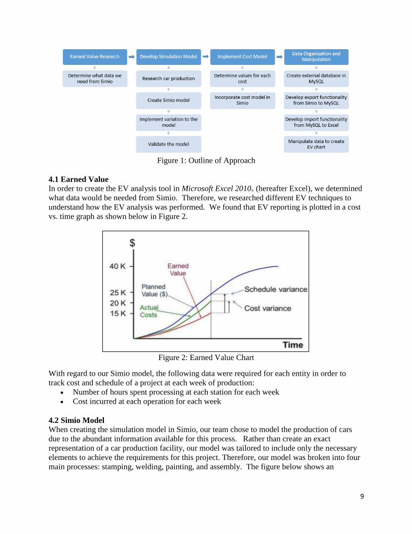
Figure 1 below shows the overall approach taken in this project. Although most of these
processes are sequential, some tasks can be performed simultaneously, such as developing the
cost model and implementing variation.
Page 9
9
Figure 1: Outline of Approach
4.1 Earned Value
In order to create the EV analysis tool in Microsoft Excel 2010® (hereafter Excel), we determined
what data would be needed from Simio. Therefore, we researched different EV techniques to
understand how the EV analysis was performed. We found that EV reporting is plotted in a cost
vs. time graph as shown below in Figure 2.
Figure 2: Earned Value Chart
With regard to our Simio model, the following data were required for each entity in order to
track cost and schedule of a project at each week of production:
Number of hours spent processing at each station for each week
Cost incurred at each operation for each week
4.2 Simio Model
When creating the simulation model in Simio, our team chose to model the production of cars
due to the abundant information available for this process. Rather than create an exact
representation of a car production facility, our model was tailored to include only the necessary
elements to achieve the requirements for this project. Therefore, our model was broken into four
main processes: stamping, welding, painting, and assembly. The figure below shows an
Page 10
10
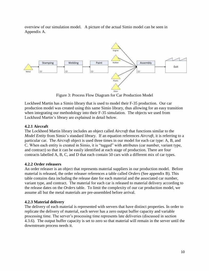
overview of our simulation model. A picture of the actual Simio model can be seen in
Appendix A.
Figure 3: Process Flow Diagram for Car Production Model
Lockheed Martin has a Simio library that is used to model their F-35 production. Our car
production model was created using this same Simio library, thus allowing for an easy transition
when integrating our methodology into their F-35 simulation. The objects we used from
Lockheed Martin’s library are explained in detail below.
4.2.1 Aircraft
The Lockheed Martin library includes an object called Aircraft that functions similar to the
Model Entity from Simio’s standard library. If an equation references Aircraft, it is referring to a
particular car. The Aircraft object is used three times in our model for each car type: A, B, and
C. When each entity is created in Simio, it is “tagged” with attributes (car number, variant type,
and contract) so that it can be easily identified at each stage of production. There are four
contracts labelled A, B, C, and D that each contain 50 cars with a different mix of car types.
4.2.2 Order releasers
An order releaser is an object that represents material suppliers in our production model. Before
material is released, the order releaser references a table called Orders (See appendix B). This
table contains data including the release date for each material and the associated car number,
variant type, and contract. The material for each car is released to material delivery according to
the release dates on the Orders table. To limit the complexity of our car production model, we
assume all but the metal materials are pre-assembled before arrival.
4.2.3 Material delivery
The delivery of each material is represented with servers that have distinct properties. In order to
replicate the delivery of material, each server has a zero output buffer capacity and variable
processing time. The server’s processing time represents late deliveries (discussed in section
4.3.6). The output buffer capacity is set to zero so that material will remain in the server until the
downstream process needs it.
Page 11
11
4.2.4 Basic and assembly stations
The basic station and the assembly station are two more objects that are specific to the Lockheed
Martin library. The basic station object is used in our model for stamping, welding, and each
paint station. Each basic station operates on a 16-hour workday with two 8-hour shifts to
simulate Lockheed Martin’s operational hours. They also have built-in process logic that
includes characteristics such as labor hours required and crew efficiency. To obtain values for
these characteristics, each basic station references a Simio data table called Station Data (see
Appendix D).
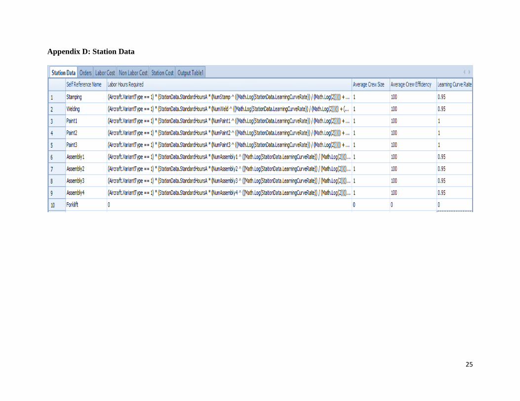
The Station Data table includes three columns that are directly used by the basic stations to
determine the processing times for each entity: labor hours required, average crew efficiency,
and average crew size. The processing times for each station are calculated using the following
equation.
(1)
The expression used for each station’s labor hours required includes three Boolean expressions
that determine the car’s variant type. When one of these three Boolean expressions is true, the
logic references the standard hours column within the Station Data table for the variant type that
is being processed. The standard hours columns include the times that each process (stamping,
welding, etc.) is expected to take for each variant type. The standard hours columns may seem
redundant at the moment, but they are necessary when implementing variability (discussed in
section 4.3). The basic station then uses Equation 1 to calculate the processing time.
The assembly station object functions very similar to the basic station in that it also operates on
the same work schedule and also references the Station Data table. The main difference is that
the assembly station requires the user to input the number of components required to begin
processing. We have set this value to five because our car requires five different materials
(engine, metal, glass, rubber, and plastic) in order to be assembled. There is a node before the
assembly stations that acts as a “gatekeeper”. The process logic at the node checks for station
availability and only passes material if the assembly station is available and other materials
already at that station are of the same car type.
Both the basic and assembly station operate with zero buffer capacities. Therefore, an entity
cannot exit a station unless there is available capacity at the following station. Lockheed
Martin’s F-35 production operates in this way because the aircraft’s large size causes a lack of
buffer space between operations.
4.2.5 Transporter
We included a transporter named “Forklift” after the assembly stations to transport the finished
cars out of the facility. A transfer node with transport logic enabled is required to make the
transporter operational. A bidirectional path connects the transfer node to the “Exit” sink so the
transporter can travel to and from the transfer node. The transporter operates on the same 16-
hour workday as the assembly and basic stations.
Page 12
12
4.3 Variability
In order to provide a measure for the cost of risk assumed in production resources, we added
many sources of variability into our simulation model. The variability was included by
implementing a learning curve, material defect rate, changes in crew size, machine reliability,
transporter availability, and material availability. We were then be able to understand how each
variability affects cost and schedule through EV analysis.
4.3.1 Learning curve
Learning curve refers to a worker’s ability to progress over time due to familiarity with a
process. This is necessary to include in our simulation because the initial labor hours required
will not accurately represent future labor hours required. This is due to improvements made by
employees over the course of time to decrease processing times. A learning curve was
implemented into the model for all basic/assembly stations except for paint. Paint does not
include a learning curve due to its process being mostly automated. The mathematical function
that models the learning curve effect is shown below in Equation 2:
(2)
Where:
Tn = time required to complete the nth unit
T1 = time required to produce the first unit
n = the cumulative number of units produced
b = log(learning curve rate)/log(2)
In order to incorporate this equation into our model, we first added a learning curve rate column
to the Station Data table so the values could easily be adjusted. Next, we added integer state
variables for each station so that the number of entities that have been processed can be
dynamically tracked. These state variables were initialized to one and an add-on process was
included for each station that added one to the station’s state variable each time an entity was
processed. With this, we were then able to incorporate Equation 2 into the labor hours required
column as seen in Appendix D. The standard hours column is representative of the time required
to produce the first unit, T1. Although the paint stations include the learning curve equation, the
learning curve rate is set to one; therefore, the labor hours required is not affected by the learning
curve equation.
4.3.2 Material defect rate
Material defects for each station were incorporated by adding two columns to the Station Data
table called Defect Rate and Defect Repair Time. The Defect Rate column uses a discrete
function that outputs 0 for non-defective units and 1 for defective units based on the defect
probability. The Defect Repair Time column reflects the time required to rework a defective
unit. An expression was then included into each labor hours required equation that added the
defect repair time if the unit was defective.
4.3.3 Crew size
As previously mentioned, the processing time for each station is calculated using the labor hours
required, average crew size, and average crew efficiency columns. Once the simulation run is
Page 13
13
initialized, the basic and assembly stations assign values for the average crew size based on the
average crew size column. This means that any variability included with this column will only
be applied once, at the simulation’s start. Therefore, in order to make this value vary throughout
the simulation, we added state variables that define the crew sizes for each station. Through add-
on processes, these state variables are assigned values using the Station Data table’s crew size
column each time an entity enters the station.
Next, we assigned each row on the average crew size column the value of one so it no longer has
an effect on the processing time. We then divided the standard hours column by the
corresponding station crew size state variable. This allows the crew size to directly affect the
labor hours required for each station. The crew size state variables are also used when
calculating the labor cost for each station.
4.3.4 Machine reliability
In order to incorporate machine reliability within each station, add-on processes and state
variables must be used because the basic and assembly stations do not include built-in reliability
logic. A Boolean state variable was created for each station. The variable is assigned a value of
0 or 1 when an entity enters the station based on the distribution in the Station Data table’s
machine reliability column. A value of 1 represents a machine failure and results in an
additional 24 hours of labor for the entity currently at the station.
We then created state variables for each station to store the station repair costs. We added an
assign step that assigns the repair cost value to the corresponding state variable. If the machine
fails at a station, the assign step randomly assigns either $1000 or $3000 to the repair cost
variable to represent both small and large repairs.
4.3.5 Transporter availability
The availability of the transporter used to transport entities from assembly to the sink is varied
using the reliability logic that is built into the object according to Figure 4.
Figure 4: Transporter Availability
A row was added to the Station Data table for the transporter so that the uptime between failures
can reference the table’s machine reliability column. This cell in the table uses a triangular
distribution to determine the number of days between failures. As seen in the figure, the time to
repair is set to 10 hours.
4.3.6 Material availability
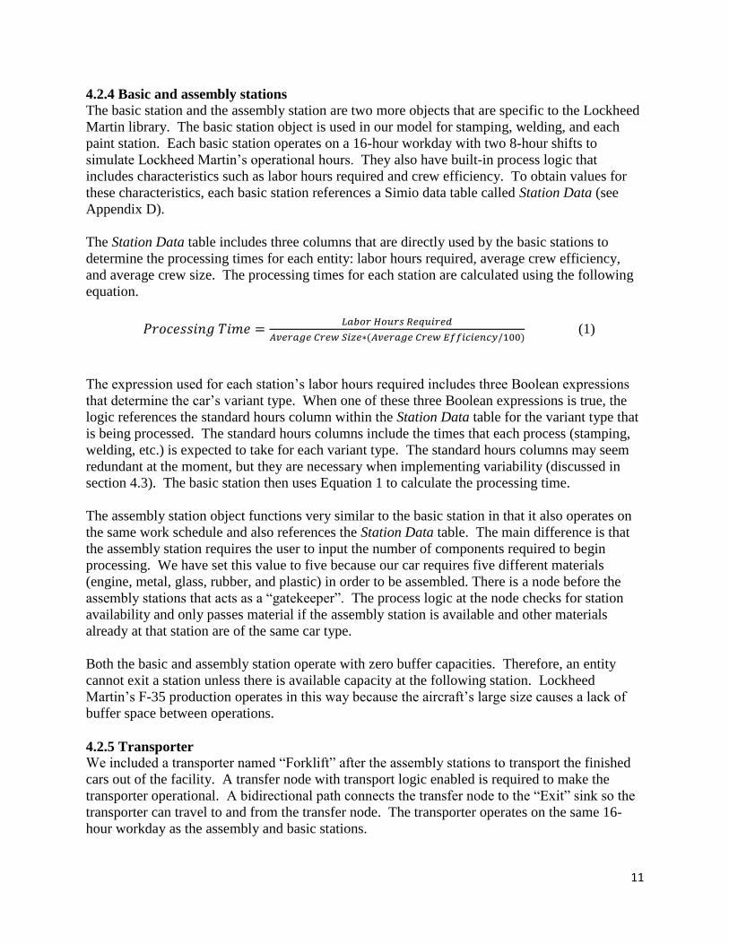
To represent late delivery of material, we added a processing time to each storage server as
shown in Figure 5. Therefore, once material is released into the system, it will not immediately
be available for use if the processing time is greater than zero.
Page 14
14
Figure 5: Material Availability
According to the above function, there is an 85% probability of no delay in delivery, a 10%
probability that there will be a 16-hour delay, and a 5% probability that a delay of 80 hours will
occur.
4.4 Model Validation
After completing the car production model with variability, various test runs were carried out to
test the goodness of the model. The goodness of the model is based upon how accurately the
performance measures such as processing times at each station and time in system for an entity
will correspond to the changes in properties of the system such as labor hours required and crew
size. We tested goodness of model by confirming our model in two major categories of
validation: structural and operational.
Structural validation checks if a model is arranged in such a manner that mimics an actual
system. So to accurately develop our car production model, we researched different production
facilities. Our team found that most car production facilities are designed in a similar manner.
The processes are usually broken into stamping, welding, painting, assembly and final
inspection. Stamping stage includes the stamping and cutting of metals to form the chassis where
the body and underbody will be mounted onto. The chassis, the underbody and the body are
welded together in the welding stage. The car at this point is just a frame, called body in white.
The body in white is inspected and sent for painting and then assembly. In the assembly
department, the interior components are added followed by the tires, batteries and
gasoline. After assembly the car goes through the final inspection before shipping. Our model is
very similar to a typical car facility except for a few features. For instance, we do not have a
specific inspection department. At each stage, the outgoing product is inspected before it moves
to the next. Also, the sub stages at each department were compressed into one. For example,
cutting metal and creating a chassis were merged into our stamping department.
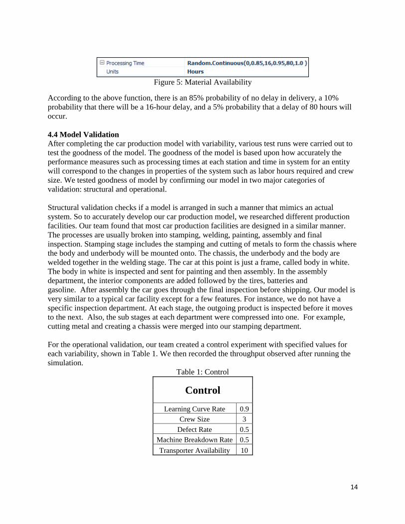
For the operational validation, our team created a control experiment with specified values for
each variability, shown in Table 1. We then recorded the throughput observed after running the
simulation.
Table 1: Control
Control
Learning Curve Rate 0.9
Crew Size 3
Defect Rate 0.5
Machine Breakdown Rate 0.5
Transporter Availability 10
Page 15
15
Next, we altered the values for each variability to see their effect on the throughput. Predictions
about the model behavior were established so that we could compare the results against the
assumptions. Table 2 below shows the altered parameters and their effects on throughput.
Table 2: Scenario Outcomes
Scenario Throughput
Control 144
Learning Curve Rate = 0.6 194
Learning Curve Rate = 0.99 101
Crew Size = 1 45
Crew Size = 5 192
Defect Rate = 0 169
Defect Rate = 1 126
Machine Breakdown Rate = 0 150
Machine Breakdown Rate = 1 136
Transporter Availability = 1 120
Transporter Availability= 60 151
Parameters like the learning curve, defect rate and the machine breakdown have an inverse
relationship with the throughput. By reducing the learning curve from 0.9 to 0.6, making the job
easier to learn, raises the throughput from 144 to 194. Alternatively, when the learning curve
increases the throughput decreases to 101. The other parameters have a direct relationship with
throughput. For example, raising the crew size increases throughput, while decreasing crew size
decreases throughput.
All outcome results were as expected, thus validating our simulation model.
4.5 Cost Model
There are five different costs integrated into our simulation model: material, labor, capital,
repair, and holding. The values used for each cost were determined from research on car
production and can be seen in Appendix C.
Material, labor, and capital costs are calculated using Simio’s cost center properties. The labor
cost is incurred per hour on-shift and is multiplied by the crew size to determine the total labor
cost for each process. The material and capital costs are incurred on a cost per job basis.
Material costs are divided amongst each process that uses the material. For example, metal costs
are split between stamping, welding, paint, and assembly because all of these stations require
metal to process. Capital costs are accumulated by determining the value of machinery at a
Page 16
16
process and dividing it by the total number of entities that use the machine during the entire
simulation. The salvage value of the machinery at the end of the simulation is also taken into
account.
The holding cost was calculated by taking the total time material spends at a process and
multiplying it by an hourly rate. For our model, the hourly rate used at each process was 10% of
the material value at the particular process. Finally, repair costs are added when a machine
breaks down as discussed in section 4.3.4.
4.6 Data Collection
The station objects in our model were grouped into two departments: metalworking and
assembly. The metalworking department includes stamping, welding, and paint, while the
assembly department includes the assembly stations.
To obtain the cost data on a weekly basis, add-on processes and state arrays were used. For both
the metal working and assembly departments, two state arrays were created: one that stores the
weekly cost for each car number and one that stores each car’s total cost for each week. An add-
on process was created for each station to calculate each cost and store them into the weekly cost
array when it exits the station. This allows multiple costs that occur in one week for the same car
to be added together within the department’s weekly cost array. A timer was added to the model
so that at the end of each week a process was triggered for each station that calculates and adds
the incurred cost to the weekly cost array if a car has not exited that station. A separate process
was then added for each department that stores the weekly cost array into the total cost array at
the end of each week. The weekly cost array was then emptied so the next week’s costs could be
stored.
The weekly schedule data was obtained using a similar process with two state arrays and add-on
processes. The main difference is that the schedule data (hours processing) is stored into the
weekly schedule array when the car completes processing, not when it exits the station. To
calculate the number of hours processing, three state variables are used for each station: one that
stores the time each car starts processing, one that stores the downtime during processing, and
one that stores the processing hours. The downtime is calculated using a separate process for
each station that adds the off-shift time while a car is at the station. The processing hours was
then calculated by subtracting the downtime and processing start time from the time it finishes
processing.
4.7 Simio Output
To create the EV chart in Excel, we required the weekly cost and schedule data from multiple
replications in our Simio model. We used an external database software, MySQL® (hereafter
MySQL), to get this data from Simio which could then be easily exported to Excel. Simio has
out-of-the-box support for MySQL that allows for reading data from or writing data to specific
tables during the simulation run using custom elements and steps.
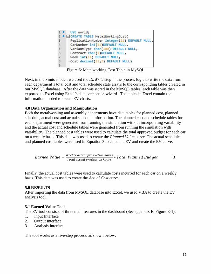
The express edition of MySQL was downloaded as required. We then created cost and schedule
tables for both the metalworking and assembly departments in MySQL. Figure 6 below shows
an example of how the tables are coded in MySQL.
Page 17
17
Figure 6: Metalworking Cost Table in MySQL
Next, in the Simio model, we used the DbWrite step in the process logic to write the data from
each department’s total cost and total schedule state arrays to the corresponding tables created in
our MySQL database. After the data was stored in the MySQL tables, each table was then
exported to Excel using Excel’s data connection wizard. The tables in Excel contain the
information needed to create EV charts.
4.8 Data Organization and Manipulation
Both the metalworking and assembly departments have data tables for planned cost, planned
schedule, actual cost and actual schedule information. The planned cost and schedule tables for
each department were generated from running the simulation without incorporating variability
and the actual cost and schedule tables were generated from running the simulation with
variability. The planned cost tables were used to calculate the total approved budget for each car
on a weekly basis. This data was used to create the Planned Value curve. The actual schedule
and planned cost tables were used in Equation 3 to calculate EV and create the EV curve.
(3)
Finally, the actual cost tables were used to calculate costs incurred for each car on a weekly
basis. This data was used to create the Actual Cost curve.
5.0 RESULTS
After importing the data from MySQL database into Excel, we used VBA to create the EV
analysis tool.
5.1 Earned Value Tool
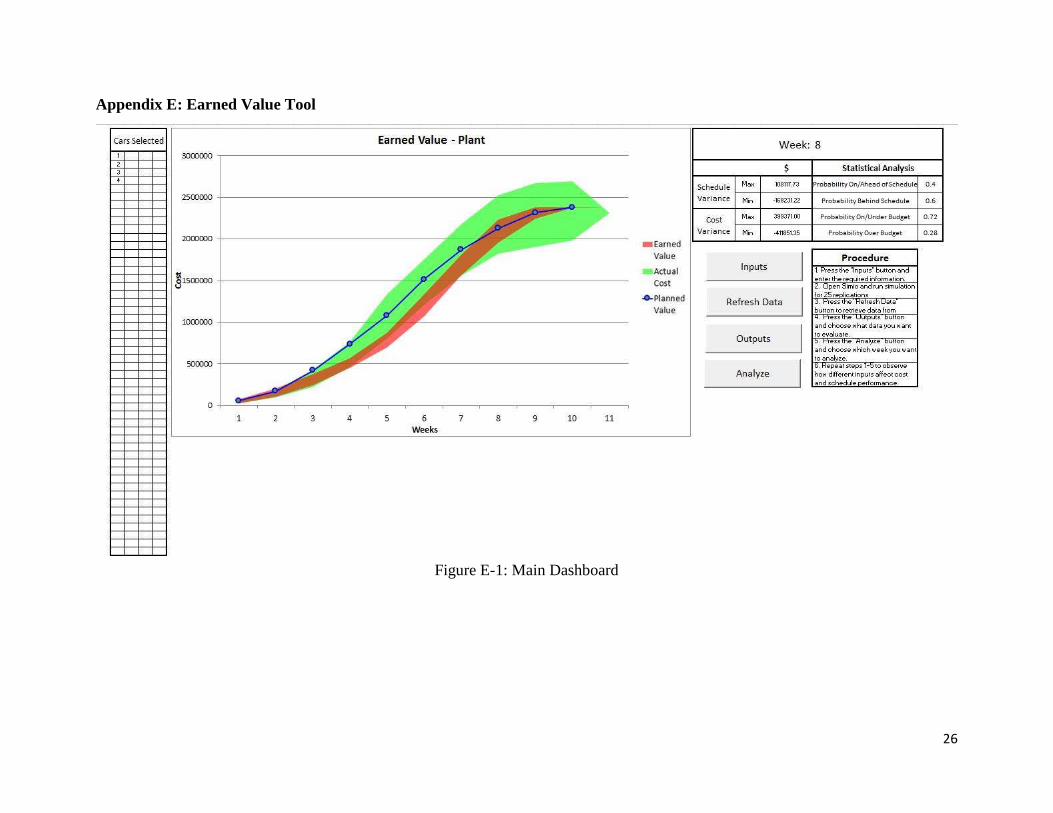
The EV tool consists of three main features in the dashboard (See appendix E, Figure E-1):
1. Input Interface
2. Output Interface
3. Analysis Interface
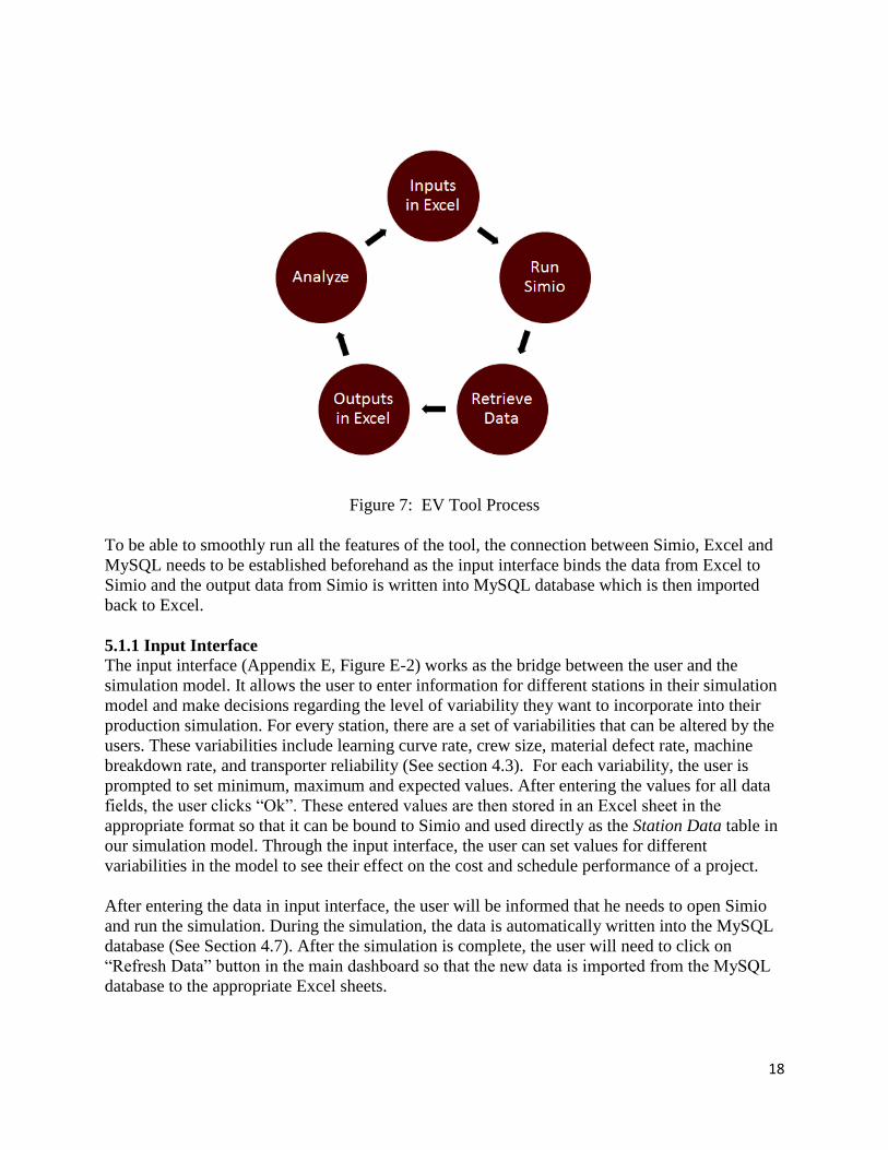
The tool works as a five-step process, as shown below:
Page 18
18
Figure 7: EV Tool Process
To be able to smoothly run all the features of the tool, the connection between Simio, Excel and
MySQL needs to be established beforehand as the input interface binds the data from Excel to
Simio and the output data from Simio is written into MySQL database which is then imported
back to Excel.
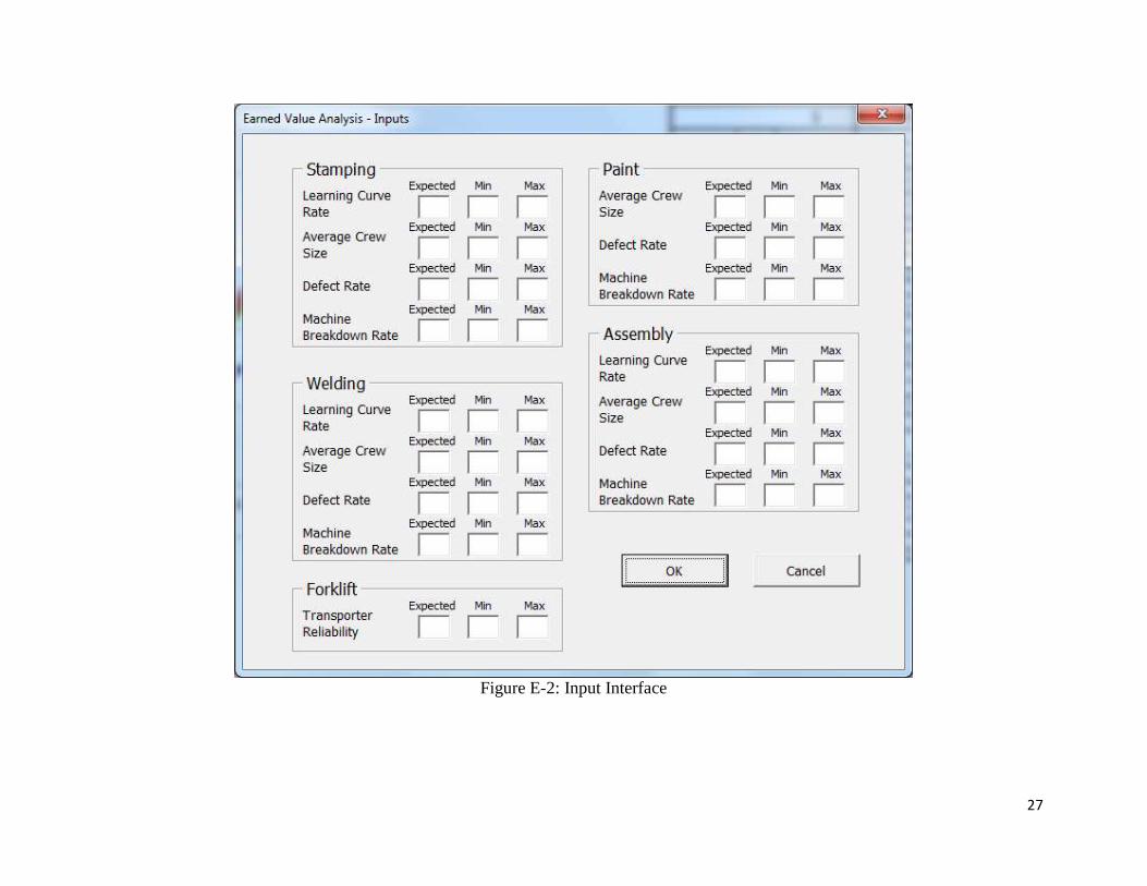
5.1.1 Input Interface
The input interface (Appendix E, Figure E-2) works as the bridge between the user and the
simulation model. It allows the user to enter information for different stations in their simulation
model and make decisions regarding the level of variability they want to incorporate into their
production simulation. For every station, there are a set of variabilities that can be altered by the
users. These variabilities include learning curve rate, crew size, material defect rate, machine
breakdown rate, and transporter reliability (See section 4.3). For each variability, the user is
prompted to set minimum, maximum and expected values. After entering the values for all data
fields, the user clicks “Ok”. These entered values are then stored in an Excel sheet in the
appropriate format so that it can be bound to Simio and used directly as the Station Data table in
our simulation model. Through the input interface, the user can set values for different
variabilities in the model to see their effect on the cost and schedule performance of a project.
After entering the data in input interface, the user will be informed that he needs to open Simio
and run the simulation. During the simulation, the data is automatically written into the MySQL
database (See Section 4.7). After the simulation is complete, the user will need to click on
“Refresh Data” button in the main dashboard so that the new data is imported from the MySQL
database to the appropriate Excel sheets.
Page 19
19
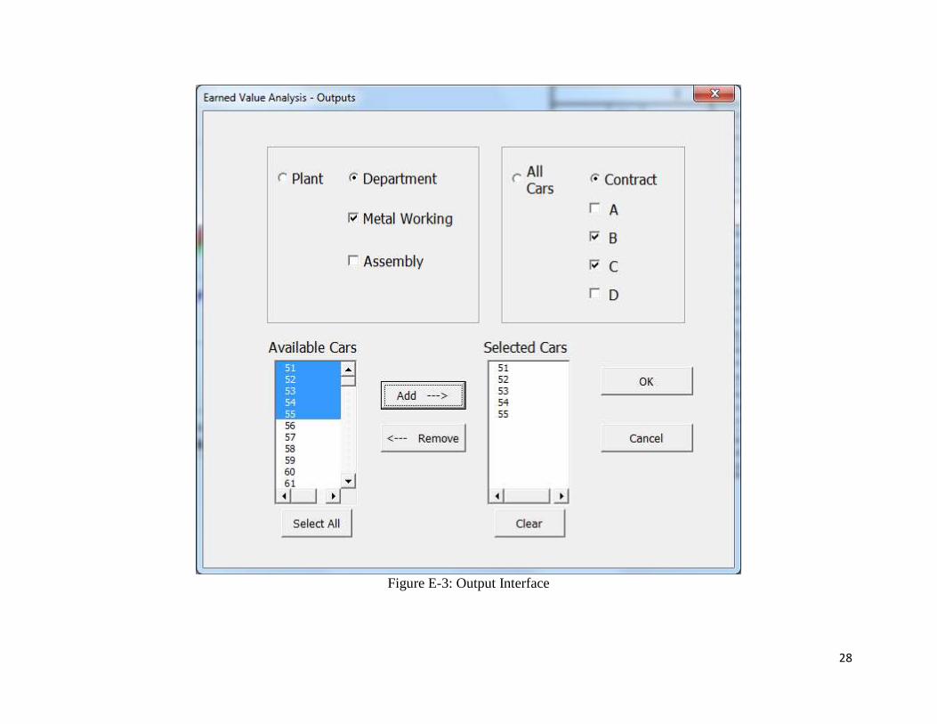
5.1.2 Output Interface
The output interface (Appendix E, Figure E-3) allows the user to generate EV charts for different
hierarchy levels in the facility. At the top of the hierarchy is the department level, consisting of
both the metalworking and assembly departments. Next is the contract level, consisting of each
contract in our model: A, B, C, and D. Finally, there is the entity level that contains each
individual car within the model.
First, the user enters the top level of the hierarchy, where he selects either “Plant”, which
includes all departments, or “Department” to individually select a department to evaluate. Then,
the user enters the contract level, where he can select either “All Cars” to populate the available
cars list box with all available cars, or “Contract” to populate the list box with available cars
within the selected contracts. Next, the entity level is entered, where the user now has the ability
to individually select which cars he would like to evaluate from the available cars. Any
combination of cars is allowed to be selected. Once the cars are selected, the user clicks the
“Add” button to move them to the selected cars list box.
After the user has made the selections, the “Ok” button is then pressed to create the EV chart in
the main dashboard (See Appendix E, Figure E-4). Since data from multiple replications was
used for the Earned Value and Actual Cost curves, area charts instead of lines are created for
better comprehension. This chart can then be analyzed using the Analyze interface.
5.1.3 Analyze Interface
The analyze interface prompts the user to enter the week for which they want to analyze the
chart. The week values that can be entered range from the start to the end of the Planned Value
curve. After the user enters a valid week number and clicks “Ok”, Cost Variance, Schedule
Variance, probabilities of being ahead or behind schedule and over or under budget are put in the
table to the right of EV chart in the main dashboard (See appendix E, Figure E-6). The user can
click on “Analyze” multiple times to analyze different weeks for the same EV chart.
5.2 Case Study
The following shows an example of how the EV analysis tool can be used to identify the risks
associated with the user’s assumptions about the model and how risk can be reduced.
5.2.1 Scenario I
The inputs entered by the user for scenario I are shown below in Tables 3 and 4.
Page 20
20
Table 3: Scenario I - Inputs Table 4: Scenario I - Inputs Cont.
After running the simulation with the above inputs, the EV graph was output for cars 1-5 across
the plant, as shown below in Figure 8.
Figure 8: Scenario I - EV Chart
As visible in the EV chart, this group of cars is behind schedule and over budget for most of the
duration. Using the analyze interface, the following data was determined for week 10.
Table 5: Scenario I - Week 10 Analysis
Page 21
21
Based on the analysis, there is zero probability that the project will be on or ahead of schedule
and zero probability that it will be on or under budget.
5.2.2 Scenario II
After analyzing the output from scenario I, the user can now make adjustments to reduce the risk
for cost and schedule performance. This is done in scenario II by adding one crew member to
each station’s crew size input. All other inputs will remain constant.
After running the simulation with the altered inputs, the EV chart was output for cars 1-5 across
the plant, as shown below in Figure 9.
Figure 9: Scenario II - EV Chart
When comparing the EV charts from each scenario, it is visible that the overall cost and schedule
performance has improved drastically. When analyzing week 10 for scenario II, the
improvements become more apparent.
Table 6: Scenario II - Week 10 Analysis
Page 22
22
The probability of being on or ahead of schedule has improved to 1, while the probability of
being on or under budget has risen to 0.96.
This case study shows how a project manager can use the EV analysis tool to forecast project
cost and schedule performance based on certain inputs and also make adjustments to these inputs
to reduce risk.
6.0 CONCLUSION
We are confident that our EV analysis tool will fulfill Lockheed Martin’s need/requirement for
simulation-based EV tool to forecast future cost and schedule performance as well as risk
associated with that forecast. Our EV analysis tool incorporates the use of Simio, MySQL and
Excel to assess Earned Value in a risk-based environment. With use of Earned Value, this tool
quantifies the risk associated with a project manager’s decisions regarding a production plan,
thus helping them identify resources to reduce those expected risks.
7.0 RECOMMENDATIONS
We recommend the use of our EV analysis tool for forecasting future cost and schedule
performances of a project with expected risk issues. To use our EV analysis tool, the cost
methodology documented in this report should be implemented into Lockheed Martin’s
simulation so that necessary cost and schedule data can be obtained.
Also, this tool could be expanded to allow the user to input real time data at any point during the
project and then run simulation from that point. This would allow EV analysis for projects that
are currently in progress.
Our team recommends that Lockheed Martin add reliability functionality to their assembly and
basic stations. This would eliminate the need to use additional state variables and process logic,
thus making it easier to implement machine reliability into the model.
To make this tool more effective, the entire process can be automated so that the user does not
have to manually open Simio and run replications after entering data in input interface. This
would save the user’s time and make the process easier to follow.
Page 23
23
8.0 APPENDIX
Appendix A
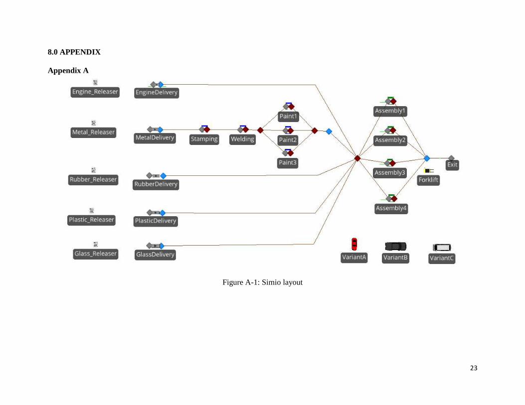
Figure A-1: Simio layout
Page 24
24
Appendix B: Orders
Appendix C
Table C-1: Material Cost Table C-2: Holding Cost
Table C-3: Capital Cost
Page 25
25
Appendix D: Station Data
Page 26
26
Appendix E: Earned Value Tool
Figure E-1: Main Dashboard
Page 27
27
Figure E-2: Input Interface
Page 28
28
Figure E-3: Output Interface
Page 29
29
Figure E-4: Sample EV chart
Page 30
30
Figure E-5: Analyze Interface
Figure E-6: EV Analysis