Tailoring Density Estimation via Reproducing Kernel Moment Matching

Le Song LE.SONG@NICTA.COM.AUXinhua Zhang XINHUA.ZHANG@NICTA.COM.AUAlex Smola ALEX.SMOLA@NICTA.COM.AUStatistical Machine Learning, NICTA, 7 London Circuit, Canberra, ACT 2601, AustraliaArthur Gretton ARTHUR.GRETTON@TUEBINGEN.MPG.DEBernhard Scholkopf BERNHARD.SCHOELKOPF@TUEBINGEN.MPG.DEMax Planck Institute for Biological Cybernetics, Spemannstr. 38, 72076 Tuebingen, Germany

AbstractMoment matching is a popular means of para-metric density estimation. We extend this tech-nique to nonparametric estimation of mixturemodels. Our approach works by embeddingdistributions into a reproducing kernel Hilbertspace, and performing moment matching in thatspace. This allows us to tailor density estima-tors to a function class of interest (i.e., for whichwe would like to compute expectations). Weshow our density estimation approach is usefulin applications such as message compression ingraphical models, and image classification andretrieval.

1. IntroductionDensity estimation is a key element of statistician’s tool-box, yet it remains a challenging problem. A popularclass of methods relies on mixture models, such as Parzenwindows (Parzen, 1962; Silverman, 1986) or mixtures ofGaussians or other basis functions (McLachlan & Basford,1988). These models are normally learned using the likeli-hood. However, density estimation is often not the ultimategoal but rather an intermediate step in solving another prob-lem. For instance, we may ultimately want to compute theexpectation of a random variable or functions thereof. Inthis case it is not clear whether likelihood is the ideal ob-jective, especially when the training sample size is small.

A second class of density estimators employ exponen-tial family models and are based on the duality betweenmaximum entropy and maximum likelihood estimation(Barndorff-Nielsen, 1978; Dudık et al., 2004; Altun &Smola, 2006). These methods match the moments of theestimators to those of the data, which helps focus the mod-els on certain aspects of the data for particular applications.However, these parametric moment based methods can be

Appearing in Proceedings of the 25 th International Conferenceon Machine Learning, Helsinki, Finland, 2008. Copyright 2008by the author(s)/owner(s).

too limited in terms of the class of distributions. Further-more, exponential families tend to require highly nontriv-ial integration of high-dimensional distributions to ensureproper normalization. We desire to overcome these draw-backs and extend this technique to a larger class of models.

In this paper, we generalize moment matching to nonpara-metric mixture models. Our major aim is to tailor thesedensity estimators for a particular function class, and pro-vide uniform convergence guarantees for approximatingthe function expectations. The key idea is if we have goodknowledge of the function class, we can tightly couple thedensity estimation with this knowledge. Rather than per-forming a full density estimation where we leave the func-tion class and subsequent operations arbitrary, we restrictour attention to a smaller set of functions and the expec-tation operator. By exploiting this kind of domain knowl-edge, we make the hard density estimation problem easier.

Our approach is motivated by the fact that distributions canbe represented as points in the marginal polytope in re-producing kernel Hilbert spaces (RKHS) (Wainwright &Jordan, 2003; Smola et al., 2007). By projecting data anddensity estimators into RKHS via kernel mean maps, wematch them in that space (also referred to as the featurespace). Choosing the kernel determines how much infor-mation about the density is retained by the kernel meanmap, and thus which aspects (e.g., moments) of a den-sity are considered important in the matching process. Thematching process, and thus our density estimation proce-dure, amounts to the solution of a convex quadratic pro-gram. We demonstrate the application of our approach inexperiments, and show that it can lead to improvements inmore complicated applications such as particle filtering andimage processing.

2. BackgroundLet X be a compact domain and X = x1, . . . , xm bea sample of size m drawn independently and identicallydistributed (iid.) from a distribution p over X . We aim tofind an approximation p of p based on the sample X .

Let H be a reproducing kernel Hilbert space (RKHS) on

Tailoring Density Estimation via Reproducing Kernel Moment Matching

X with kernel k : X × X 7→ R and associated featuremap φ : X 7→ H such that k(x, x′) = 〈φ(x), φ(x′)〉H.By design H has the reproducing property, that is, for anyf ∈ H we have f(x) = 〈f, k(x, ·)〉H. A kernel k is calleduniversal if H is dense in the space of bounded continu-ous functions C0(X ) on the compact domain X in the L∞norm (Steinwart, 2002). Examples of such kernels includeGaussian kernel exp(−‖x− x′‖2 /2θ2) and Laplace ker-nel exp(−‖x− x′‖ /2θ2).

The marginal polytope is the range of the expectation of thefeature map φ under all distributions in a set P , i.e.,M :=µ[p]|p ∈ P, µ[p] := Ex∼p [φ(x)] (Wainwright & Jordan,2003). The map µ : P 7→ H associates a distribution to anelement in the RKHS. For universal kernels, the elementsof the marginal polytope uniquely determine distributions:

Theorem 1 (Gretton et al. (2007)) Let k be universal andP denote the set of Borel probability measures p on X withEx∼p [k(x, x)] <∞. Then the map µ is injective.

3. Kernel Moment MatchingGiven a finite sample X from p, µ[p] can be approximatedby the empirical mean map µ[X] := 1

m

∑mi=1 φ(xi). This

suggests that a good estimate p of p should be chosen suchthat µ[p] matches µ[X]: this is the key idea of the paper.The flow of reasoning works as follows:

density p→ sample X → empirical mean µ[X]→ density estimation via µ[p] ≈ µ[X] (1)

The first line of this reasoning was established in (Al-tun & Smola, 2006, Theorem 15). Let Rm(H, p) be theRademacher average (Bartlett & Mendelson, 2002) associ-ated with p andH via

Rm(H, p) := 1mEXEω

[sup‖f‖H≤1

∣∣∣∑m

i=1ωif(xi)

∣∣∣] .

where ω ∈ ±1 is uniformly random. We use it to boundthe deviation between empirical means and expectations:Theorem 2 (Altun & Smola (2006)) Assume ‖f‖∞ ≤ Rfor all f ∈ H with ‖f‖H ≤ 1. Then for ε > 0with probability at least 1 − exp(−ε2mR−2/2) we have‖µ[p]− µ[X]‖H ≤ 2Rm(H, p) + ε.

This ensures that µ[X] is a good proxy for µ[p]. To carryout the last step of (1) we assume the density estimator p isa mixture of a set of candidate densities pi (or prototypes):

p =∑n

i=1αipi where α>1 = 1 and αi ≥ 0, (2)

where 1 is a vector of all ones. Here the goal is to obtaingood estimates for the coefficients αi and to obtain perfor-mance guarantees which specify how well p is capable ofestimating p. This can be cast as an optimization problem:

minα‖µ[X]− µ[p]‖2H s.t. α>1 = 1 , αi ≥ 0. (3)

To prevent overfitting, we add a regularizer Ω[α], such as

12 ‖α‖

2, and weight it by a regularization constant λ > 0.Using the expansion of p in (2) we obtain a quadratic pro-gram (QP) for α

minα

12α>(Q + λI)α− l>α s.t. α>1 = 1 , αi ≥ 0, (4)

where I is the identity matrix. Q ∈ Rn×n and l ∈ Rn aregiven byQij = 〈µ[pi], µ[pj ]〉H = Ex∼pi,x′∼pj

[k(x, x′)] , (5)

lj = 〈µ[X], µ[pj ]〉H = 1m

∑m

i=1Ex∼pj [k(xi, x)] . (6)

By construction Q 0 is positive semidefinite, hence theprogram (4) is convex. We will discuss examples of kernelsk and prototypes pi where Q and l have closed form in Sec-tion 5. In many cases, the prototypes pi also contain tun-able parameters. We can also optimize them via gradientmethods. Before doing so, we first explain our theoreticalbasis for tailoring density estimators.

4. Tailoring Density EstimatorsGiven functions f ∈ H, a key question is to bound howwell the expectations of f with respect to p can be approx-imated by p. We have the following lemma:

Lemma 3 Let ε > 0 and ε′ := ‖µ[X]− µ[p]‖H. Underthe assumptions of Theorem 2 we have with probability atleast 1− exp(−ε2mR−2/2)

sup‖f‖H≤1

|Ex∼p[f(x)]− Ex∼p[f(x)]| ≤ 2Rm(H, p) + ε + ε′.

Proof In the RKHS, we have Ex∼p[f(x)] = 〈f, µ[p]〉Hand Ex∼p[f(x)] = 〈f, µ[p]〉H. Hence the LHS of thebound equates to sup‖f‖H≤1 | 〈µ[p]− µ[p], f〉 |, which isgiven by ‖µ[p]− µ[p]‖H. Using the triangle inequality, ourassumption on µ[p] and Theorem 2 completes the proof.

This means that we have good control over the behavior ofthe expectations, as long as the function class is “smooth”on X in terms of the Rademacher average. It also meansthat ‖µ[X]− µ[p]‖H is a sensible objective to minimize ifwe are only interested in approximating well the expecta-tions over functions f .

This bound also provides the basis for tailoring density es-timators. Essentially, if we have good knowledge of thefunction class used in an application, we can choose thecorresponding RKHS or the mean map. This is equivalentto filtering the data and extracting only certain moments.Then the density estimator p can focus on matching p onlyup to these moments.

5. ExamplesWe now give concrete examples of density estimation. Anumber of existing methods are special cases of our setting.

Discrete Prototype or Discrete Kernel The simplestcase is to represent p by a convex combination of Dirac

Tailoring Density Estimation via Reproducing Kernel Moment Matching

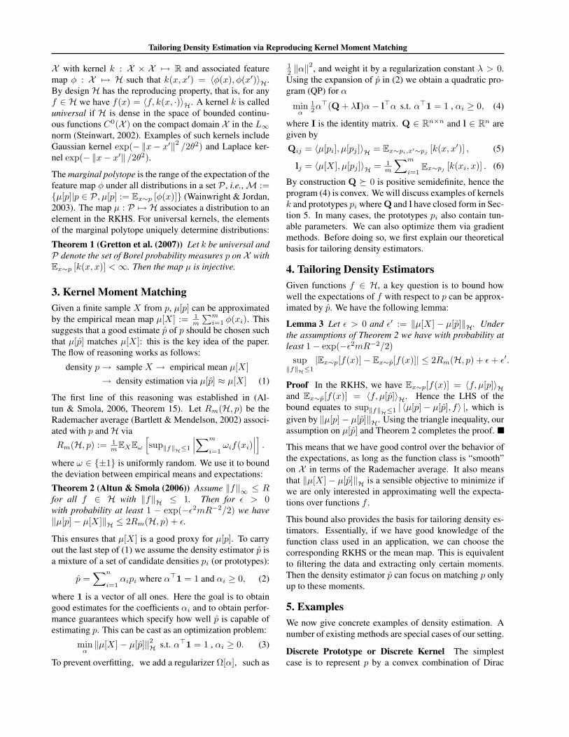
Table 1. Expansions for Qij and lj when using Gaussian prototypes and various kernels in combination. Let c := 〈xi, xj〉+ 1.Kernel Qij lj

Linear kernel˙x, x′

¸〈xi, xj〉 1

m

Pmi=1 〈xi, xj〉

Degree 2 polynomial kernel (˙x, x′

¸+ 1)2 c2 + tr ΣiΣj + x>i Σjxi + x>j Σixj

1m

Pmi=1(c

2 + x>i Σjxi)

Degree 3 polynomial kernel (˙x, x′

¸+ 1)3 c3 + 6x>i ΣiΣjxj + 3c(tr ΣiΣj + x>i Σjxi + x>j Σixj)

1m

Pmi=1(c

3 + 3cx>i Σjxi)

Gaussian RBF kernel e− 1

2θ2 ‖x−x′‖2θd

˛Σi + Σj + θ2I

˛− 12 e

− 12‖xi−xj‖2(Σi+Σj+θ2I) 1

m θd˛Σj + θ2I

˛− 12

Pmi=1 e

− 12‖xi−xj‖2(Σj+θ2I)

measures pi(x) = δxi . Particle filters (Doucet et al., 2001)use this choice when approximating distributions. For in-stance, we could choose xi to be the set of training points.In this case Q defined in (5) equals the kernel matrix and lis the vector of empirical kernel averages:

Qij = k(xi, xj) and lj = 1m

∑m

i=1k(xi, xj). (7)

The key difference between an unweighted set as used inparticle filtering and our setting is that our expansion isspecifically optimized towards good estimates with respectto functions drawn fromH.

The problem of data squashing (DuMouchel et al., 1999)can likewise be seen as a special case of kernel meanmatching. Here one aims to approximate a potentially largeset X by a smaller set X ′ = (x1, α1), . . . , (xn, αn) ofweighted observations. We want to discard X and only re-tain X ′ for all further processing. If ‖µ[X] − µ[X ′]‖H issmall, we expect X ′ to be a good proxy for X .

Instead of using generic kernels k and discrete measuresδxi as prototypes for density estimation, we may reversetheir roles. That is, we may pick generic densities pi and aDirac kernel k(x, x′) = δ(x = x′). Note this is only welldefined for discrete domains X .1 In this case the mean op-erator simply maps a distribution into itself and we obtain〈µ[p], µ[p′]〉H =

∫X p(x)p′(x)dx. Using (5) we have

Qij =∫X

pi(x)pj(x)dx and lj = 1m

∑m

i=1pj(xi). (8)

Gaussian Prototype In general we will neither pick dis-crete prototypes nor discrete kernels for density estimation.We now give explicit expressions for Gaussian prototypes

pi(x) = (2π)−d2 |Σi|−

12 exp

(− 1

2 ‖x− xi‖2Σi

), (9)

where d is the dimension of the data, Σi 0 is a covariancematrix, and ‖x− x′‖2Σi

:= (x − x′)>Σ−1i (x − x′) is the

squared Mahalanobis distance. When used in conjunctionwith different kernels, we have the expansions in Table 1.

Other Prototypes and Kernels Other combinations ofkernels and prototypes also lead to closed form expansions.For instance, similar expressions also holds for a Laplaciankernel. However, this involves more tedious integrals of theform

∫e−λ(|x|+|x−a|)dx = λ−1 + e−λ|a|. Another exam-

ple is to use indicator functions on unit intervals centeredat xi as pi and a Gaussian RBF kernel. In this case, both Qand l can be expressed using the error function (erf).

1On continuous domains such a kernel does not correspond toan RKHS since the point evaluation is not continuous.

Furthermore, Jebara et al. (2004) introduced kernels onprobability functions which effectively used definition (5).While they were not motivated by the connection betweenkernels and density estimation, their results for rich classesof densities, such as HMMs, can be used directly to com-pute our Q and l.

6. Related WorkOur work is related to the density estimators of Vapnik &Mukherjee (2000) and Shawe-Taylor & Dolia (2007). Themain difference lies in the function space chosen to mea-sure the approximation properties. The former uses theBanach space of functions of bounded variation, while thelatter uses the space L1(q), where q denotes a distributionover test functions. For spherically invariant distributionsover test functions our approach and the latter approach areidentical, with a key difference (to our advantage) that ouroptimization is a simple QP which does not require con-straint sampling to make the optimization feasible.

Support Vector Density Estimation The model of Vap-nik & Mukherjee (2000) can be summarized as follows: letF [p] be the cumulative distribution function of p and letF [X] be its empirical counterpart. Assume p is given by(2), and that we have a regularizer Ω[α] as previously dis-cussed. In this case the Support Vector Density Estimationproblem can be written as

minα feasible

1m

∑m

i=1|F [p](xi)− F [X](xi)|+ λΩ[α]. (10)

That is, we minimize the `1 distance between the empir-ical and estimated cumulative distribution functions whenevaluated on the set of observations X .

To integrate this into our framework we need to extendour setting from Hilbert spaces to Banach spaces. De-note by B a Banach space, let X be a domain furnishedwith probability measures p, p′, and let φ : X 7→ B bea feature map into B. Analogously, we define the meanmap µ : P 7→ B as µ[p] := Ex∼p(x) [φ(x)]. More-over, we define a distance between distributions p and p′

via D(p, p′) := ‖µ[p]− µ[p′]‖B. If we choose φ(x) =(χ(−∞,x](x1), . . . , χ(−∞,x](xm)

)>where χ is the indica-

tor function, and use the `m1 norm on φ we recover SV den-

sity estimation as a special case.

Expected Deviation Estimation Shawe-Taylor & Dolia(2007) defined a distance between distributions as follows:let H be a set of functions on X and q be a probabilitydistribution over F . Then the distance between two distri-butions p and p′ is given by

Tailoring Density Estimation via Reproducing Kernel Moment Matching

D(p, p′) := Ef∼q(f) |Ex∼p[f(x)]− Ex∼p′ [f(x)]| . (11)

That is, we compute the average distance between p and p′

with respect to a distribution of test functions.Lemma 4 Let H be a reproducing kernel Hilbert space,f ∈ H, and assume q(f) = q(‖f‖H) with finiteEf∼q[‖f‖H]. Then D(p, p′) = C ‖µ[p]− µ[p′]‖H forsome constant C which depends only onH and q.Proof Note that by definition Ex∼p[f(x)] = 〈µ[p], f〉H.Using linearity of the inner product, Equation (11) equals∫

|〈µ[p]− µ[p′], f〉H|dq(f)

= ‖µ[p]− µ[p′]‖H∫ ∣∣∣∣⟨ µ[p]− µ[p′]

‖µ[p]− µ[p′]‖H, f

⟩H

∣∣∣∣ dq(f),

where the integral is independent of p, p′. To see this, notethat for any p, p′, µ[p]−µ[p′]

‖µ[p]−µ[p′]‖His a unit vector which can

be turned into, say, the first canonical basis vector by a ro-tation which leaves the integral invariant, bearing in mindthat q is rotation invariant.

The above result covers a large number of interesting func-tion classes. To go beyond Hilbert spaces, let φ : X 7→ Bbe the transformation from x into f(x) for all f ∈ H and‖z‖B := Ef∼q(f)[|zf |] be the L1(q) norm. Then (11) canalso be written as ‖µ[p]− µ[p′]‖B, where µ is the meanmap into Banach spaces. Its main drawback is the nontriv-ial computation for constraint sampling (de Farias & Roy,2004) and the additional uniform convergence reasoningrequired. In Hilbert spaces no such operations are needed.

7. ExperimentsWe focus on two aspects: first, our method performs wellas a density estimator per se; and second, it can be tailoredtowards the expectation over a particular function class.

7.1. Methods for ComparisonGaussian Mixture Model (GMM)2 The density wasrepresented as a convex sum of Gaussians. GMM was ini-tialized with k-means clustering. The centers, covariancesand mixing proportions of the Gaussians were optimizedusing the EM algorithm. We used diagonal covariancesin all our experiments. We always employed 50 randomrestarts for k-means, and returned the results from the bestrestart.Parzen Windows (PZ) The density was represented asan average of a set of normalized RBF functions, witheach centered on a data point. The bandwidths of the RBFfunctions were identical and tuned via the likelihood usingleave-one-out cross validation.Reduced Set Density Estimation (RSDE)3 Girolami &He (2003) compressed a Parzen window estimator usingRBF functions of larger bandwidths. The reduced represen-

2GMM codes from: http://www.datalab.uci.edu/resources/gmm/3PZ and RSDE from: http://ttic.uchicago.edu/∼ihler/code/

50 150 250 350 4503.8

3.9

4

4.1

4.2

Training Sample Size

Neg

ativ

e Lo

g Li

kelih

ood GMM

PZRSDEKMM

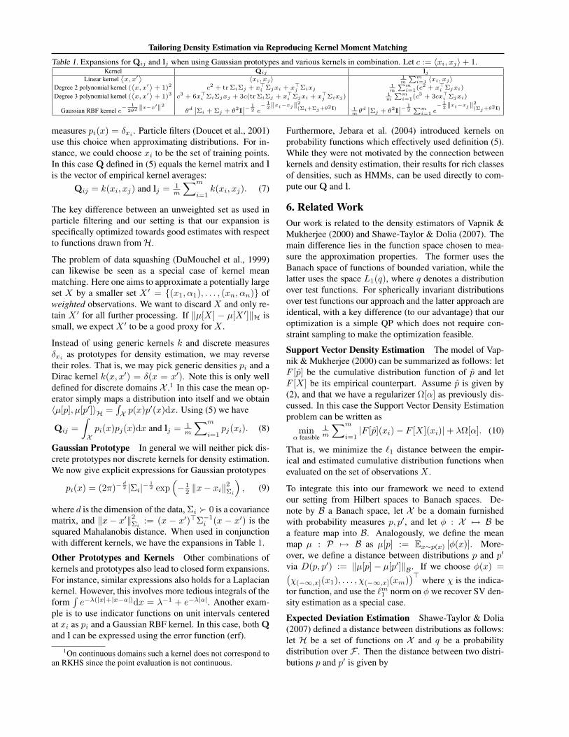
Figure 1. Left: Negative log-likelihood using a mixture of 3Gaussians. The height of the bars represents the median of thescores from 100 repeats, and the whiskers correspond to thequartiles. We mark the best method with a black dot above thewhiskers. Right: Sparsity of KMM solution. Blue dots are datapoints. Red circles represent prototypes selected by KMM. Thesize of a circle is proportional to the magnitude of its weight αi.

tation was produced by minimizing an integrated squareddistance between the two densities.Kernel Moment Matching (KMM) In applying ourmethod, we used Gaussians with diagonal covariances asour prototypes pi. The regularization parameter λ in ouralgorithm was fixed at 10−10 throughout. Since KMM maybe tailored for different RKHS, we instantiated it with thefour different kernels in Table 1. We denote them as LIN,POL2, POL3 and RBF, respectively. Our choice of kernelcorresponded to the function class where we evaluated theexpectations. The initialization of the prototypes will befurther discussed below.

7.2. Evaluation CriterionWe compared various density estimators in terms of twocriteria: negative log-likelihood and discrepancy betweenfunction expectations on test data. Since different algo-rithms are optimized using different criteria, we expect thateach will win with respect to the criterion it employs. Thebenefit of our density estimator is that we can explicitlytailor for different classes of functions. For this reason, wewill focus on the second criterion.

Given a function f , the discrepancy between function ex-pectations is computed as follows: (i) Evaluate functionexpectation using test points, i.e., 1

m

∑mi=1 f(xi); (ii) Eval-

uate function expectation using estimated density p, i.e.,Ex∼p[f(x)]. (iii) Calculate

∣∣ 1m

∑mi=1 f(xi)− Ex∼p[f(x)]

∣∣and normalize it by

∣∣ 1m

∑mi=1 f(xi)

∣∣.We will compare various methods either by repeated ran-dom instantiation or random split of the data (which wewill make clear in context). For both cases, we will per-form paired sign tests at the significance level of 0.01 on theresults obtained from the randomizations. We will alwayspresent the median of the results in subsequent tables, andhighlight in boldface those statistically equivalent methodsthat are significantly better than the rest.

7.3. Synthetic DatasetIn this experiment, we use synthetic datasets to comparevarious methods as the sample size changes. We also show

Tailoring Density Estimation via Reproducing Kernel Moment Matching

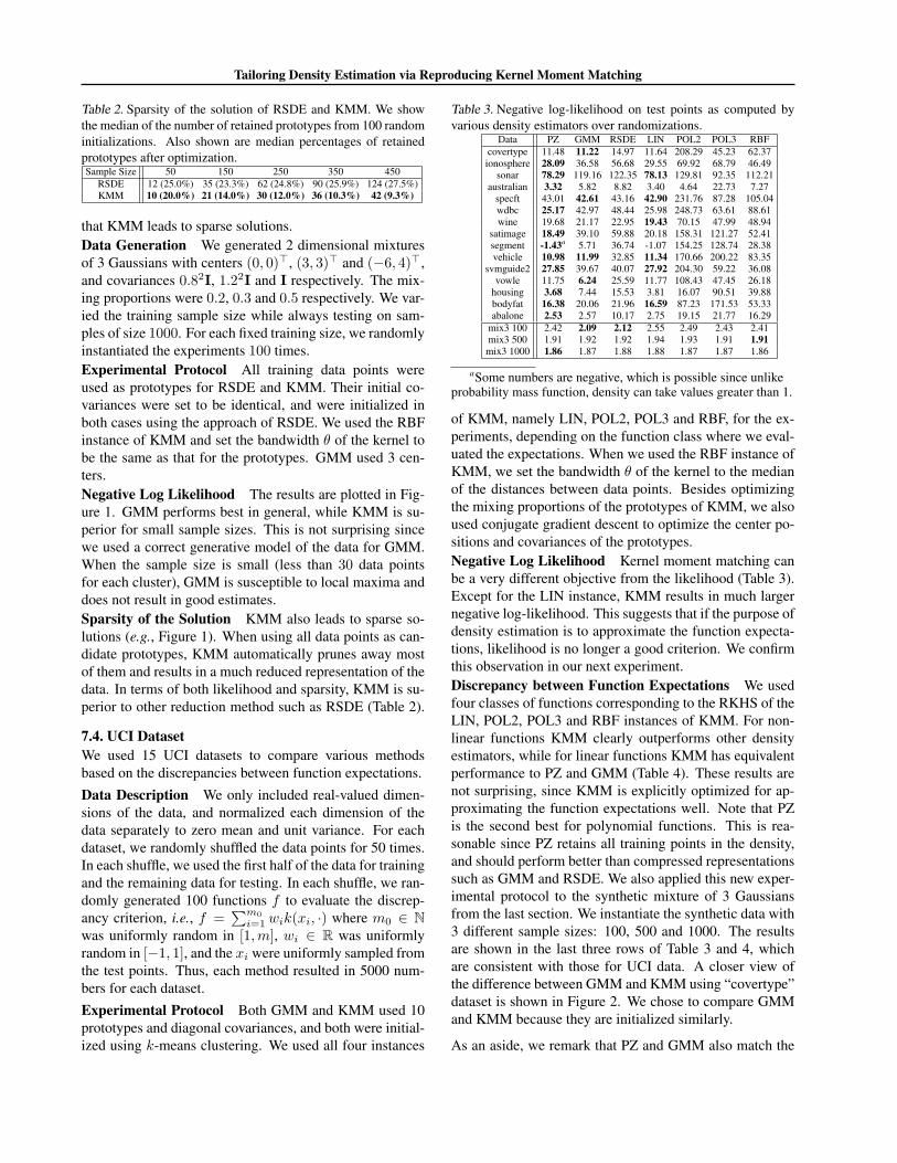
Table 2. Sparsity of the solution of RSDE and KMM. We showthe median of the number of retained prototypes from 100 randominitializations. Also shown are median percentages of retainedprototypes after optimization.Sample Size 50 150 250 350 450

RSDE 12 (25.0%) 35 (23.3%) 62 (24.8%) 90 (25.9%) 124 (27.5%)KMM 10 (20.0%) 21 (14.0%) 30 (12.0%) 36 (10.3%) 42 (9.3%)

that KMM leads to sparse solutions.Data Generation We generated 2 dimensional mixturesof 3 Gaussians with centers (0, 0)>, (3, 3)> and (−6, 4)>,and covariances 0.82I, 1.22I and I respectively. The mix-ing proportions were 0.2, 0.3 and 0.5 respectively. We var-ied the training sample size while always testing on sam-ples of size 1000. For each fixed training size, we randomlyinstantiated the experiments 100 times.Experimental Protocol All training data points wereused as prototypes for RSDE and KMM. Their initial co-variances were set to be identical, and were initialized inboth cases using the approach of RSDE. We used the RBFinstance of KMM and set the bandwidth θ of the kernel tobe the same as that for the prototypes. GMM used 3 cen-ters.Negative Log Likelihood The results are plotted in Fig-ure 1. GMM performs best in general, while KMM is su-perior for small sample sizes. This is not surprising sincewe used a correct generative model of the data for GMM.When the sample size is small (less than 30 data pointsfor each cluster), GMM is susceptible to local maxima anddoes not result in good estimates.Sparsity of the Solution KMM also leads to sparse so-lutions (e.g., Figure 1). When using all data points as can-didate prototypes, KMM automatically prunes away mostof them and results in a much reduced representation of thedata. In terms of both likelihood and sparsity, KMM is su-perior to other reduction method such as RSDE (Table 2).

7.4. UCI DatasetWe used 15 UCI datasets to compare various methodsbased on the discrepancies between function expectations.

Data Description We only included real-valued dimen-sions of the data, and normalized each dimension of thedata separately to zero mean and unit variance. For eachdataset, we randomly shuffled the data points for 50 times.In each shuffle, we used the first half of the data for trainingand the remaining data for testing. In each shuffle, we ran-domly generated 100 functions f to evaluate the discrep-ancy criterion, i.e., f =

∑m0i=1 wik(xi, ·) where m0 ∈ N

was uniformly random in [1,m], wi ∈ R was uniformlyrandom in [−1, 1], and the xi were uniformly sampled fromthe test points. Thus, each method resulted in 5000 num-bers for each dataset.

Experimental Protocol Both GMM and KMM used 10prototypes and diagonal covariances, and both were initial-ized using k-means clustering. We used all four instances

Table 3. Negative log-likelihood on test points as computed byvarious density estimators over randomizations.

Data PZ GMM RSDE LIN POL2 POL3 RBFcovertype 11.48 11.22 14.97 11.64 208.29 45.23 62.37ionosphere 28.09 36.58 56.68 29.55 69.92 68.79 46.49

sonar 78.29 119.16 122.35 78.13 129.81 92.35 112.21australian 3.32 5.82 8.82 3.40 4.64 22.73 7.27

specft 43.01 42.61 43.16 42.90 231.76 87.28 105.04wdbc 25.17 42.97 48.44 25.98 248.73 63.61 88.61wine 19.68 21.17 22.95 19.43 70.15 47.99 48.94

satimage 18.49 39.10 59.88 20.18 158.31 121.27 52.41segment -1.43a 5.71 36.74 -1.07 154.25 128.74 28.38vehicle 10.98 11.99 32.85 11.34 170.66 200.22 83.35

svmguide2 27.85 39.67 40.07 27.92 204.30 59.22 36.08vowle 11.75 6.24 25.59 11.77 108.43 47.45 26.18

housing 3.68 7.44 15.53 3.81 16.07 90.51 39.88bodyfat 16.38 20.06 21.96 16.59 87.23 171.53 53.33abalone 2.53 2.57 10.17 2.75 19.15 21.77 16.29

mix3 100 2.42 2.09 2.12 2.55 2.49 2.43 2.41mix3 500 1.91 1.92 1.92 1.94 1.93 1.91 1.91

mix3 1000 1.86 1.87 1.88 1.88 1.87 1.87 1.86

aSome numbers are negative, which is possible since unlikeprobability mass function, density can take values greater than 1.

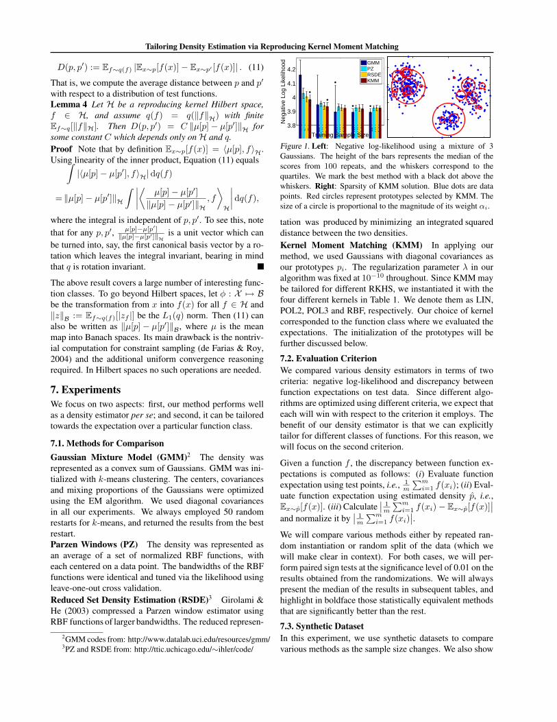
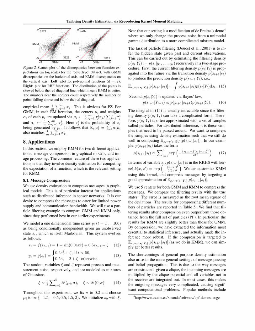
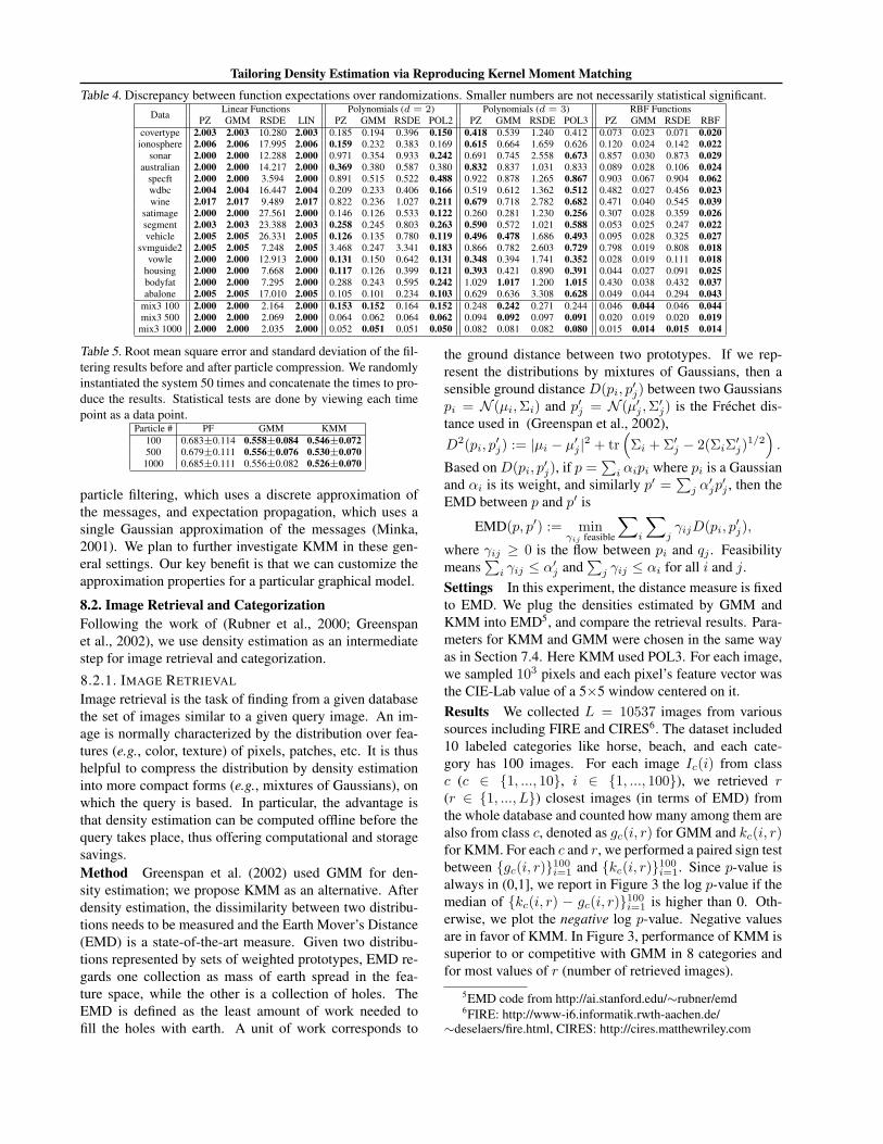
of KMM, namely LIN, POL2, POL3 and RBF, for the ex-periments, depending on the function class where we eval-uated the expectations. When we used the RBF instance ofKMM, we set the bandwidth θ of the kernel to the medianof the distances between data points. Besides optimizingthe mixing proportions of the prototypes of KMM, we alsoused conjugate gradient descent to optimize the center po-sitions and covariances of the prototypes.Negative Log Likelihood Kernel moment matching canbe a very different objective from the likelihood (Table 3).Except for the LIN instance, KMM results in much largernegative log-likelihood. This suggests that if the purpose ofdensity estimation is to approximate the function expecta-tions, likelihood is no longer a good criterion. We confirmthis observation in our next experiment.Discrepancy between Function Expectations We usedfour classes of functions corresponding to the RKHS of theLIN, POL2, POL3 and RBF instances of KMM. For non-linear functions KMM clearly outperforms other densityestimators, while for linear functions KMM has equivalentperformance to PZ and GMM (Table 4). These results arenot surprising, since KMM is explicitly optimized for ap-proximating the function expectations well. Note that PZis the second best for polynomial functions. This is rea-sonable since PZ retains all training points in the density,and should perform better than compressed representationssuch as GMM and RSDE. We also applied this new exper-imental protocol to the synthetic mixture of 3 Gaussiansfrom the last section. We instantiate the synthetic data with3 different sample sizes: 100, 500 and 1000. The resultsare shown in the last three rows of Table 3 and 4, whichare consistent with those for UCI data. A closer view ofthe difference between GMM and KMM using “covertype”dataset is shown in Figure 2. We chose to compare GMMand KMM because they are initialized similarly.

As an aside, we remark that PZ and GMM also match the

Tailoring Density Estimation via Reproducing Kernel Moment Matching

−5 GMM 2

−5

KMM

2

3223

1777

−7 GMM 0

−7

KMM

0

3011

1989

Figure 2. Scatter plot of the discrepancies between function ex-pectations (in log scale) for the ‘covertype’ dataset, with GMMdiscrepancies on the horizontal axis and KMM discrepancies onthe vertical axis. Left: plot for polynomial functions (d = 2);Right: plot for RBF functions. The distribution of the points isskewed below the red diagonal line, which means KMM is better.The numbers near the corners count respectively the number ofpoints falling above and below the red diagonal.

empirical mean 1m

∑mj=1 xj . This is obvious for PZ. For

GMM, in each EM iteration, the centers µi and weightsαi of each pi are updated via µi ←

∑mj=1 τ i

jxj/∑m

j=1 τ ij

and αi ← 1m

∑mj=1 τ i

j . Here τ ij is the probability of xj

being generated by pi. It follows that Ep[x] =∑

i αiµi

also matches 1m

∑mj=1 xj .

8. ApplicationsIn this section, we employ KMM for two different applica-tions: message compression in graphical models, and im-age processing. The common feature of these two applica-tions is that they involve density estimation for computingthe expectation of a function, which is the relevant settingfor KMM.

8.1. Message CompressionWe use density estimation to compress messages in graph-ical models. This is of particular interest for applicationssuch as distributed inference in sensor networks. It is ourdesire to compress the messages to cater for limited powersupply and communication bandwidth. We will use a par-ticle filtering example to compare GMM and KMM only,since they performed best in our earlier experiments.

We model a one dimensional time series yt (t = 1 . . . 100)as being conditionally independent given an unobservedstate st, which is itself Markovian. This system evolvesas follows:

st = f(st−1) = 1 + sin(0.04πt) + 0.5st−1 + ξ (12)

yt = g(st) =

0.2s2

t + ζ, if t < 50,

0.5st − 2 + ζ, otherwise.(13)

The random variables ξ and ζ represent process and mea-surement noise, respectively, and are modeled as mixturesof Gaussians,

ξ ∼ 15

∑5

i=1N (µi, σ), ζ ∼ N (0, σ). (14)

Throughout this experiment, we fix σ to 0.2 and chooseµi to be −1.5,−0.5, 0.5, 1.5, 2. We initialize s0 with ξ.

Note that our setting is a modification of de Freitas’s demo4

where we only change the process noise from a unimodalgamma distribution to a more complicated mixture model.

The task of particle filtering (Doucet et al., 2001) is to in-fer the hidden state given past and current observations.This can be carried out by estimating the filtering densityp(st|Yt) := p(st|y1, . . . , yt) recursively in a two-stage pro-cedure. First, the current filtering density p(st|Yt) is prop-agated into the future via the transition density p(st+1|st)to produce the prediction density p(st+1|Yt), i.e.,

Est∼p(st|Yt)[p(st+1|st)] :=∫

p(st+1|st)p(st|Yt)dst. (15)

Second, p(st|Yt) is updated via Bayes’ law,p(st+1|Yt+1) ∝ p(yt+1|st+1)p(st+1|Yt). (16)

The integral in (15) is usually intractable since the filter-ing density p(st|Yt) can take a complicated form. There-fore, p(st|Yt) is often approximated with a set of samplescalled particles. For distributed inference, it is these sam-ples that need to be passed around. We want to compressthe samples using density estimation such that we still dowell in computing Est∼p(st|Yt)[p(st+1|st)]. In our exam-ple, p(st+1|st) takes the form

p(st+1|st) ∝∑5

i=1exp

(− (st+1−f(st)−µi)

2

2σ2

). (17)

In terms of variable st, p(st+1|st) is in the RKHS with ker-nel k(x, x′) = exp

(− (x−x′)2

2(2σ)2

). We can customize KMM

using this kernel, and compress messages by targeting agood approximation of Est∼p(st|Yt)[p(st+1|st)].

We use 5 centers for both GMM and KMM to compress themessages. We compare the filtering results with the truestates. The error is measured as the root mean square ofthe deviations. The results for compressing different num-bers of particles are reported in Table 5. We find that fil-tering results after compression even outperform those ob-tained from the full set of particles (PF). In particular, theresults for KMM are slightly better than those for GMM.By compression, we have extracted the information mostessential to statistical inference, and actually made the in-ference more robust. If the compression is targeted toEst∼p(st|Yt)[p(st+1|st)] (as we do in KMM), we can sim-ply get better results.

The shortcomings of general purpose density estimationalso arise in the more general settings of message passingand belief propagation. This is due to the way messagesare constructed: given a clique, the incoming messages aremultiplied by the clique potential and all variables not inthe receiver are integrated out. In most cases, this makesthe outgoing messages very complicated, causing signif-icant computational problems. Popular methods include

4http://www.cs.ubc.ca/∼nando/software/upf demos.tar.gz

Tailoring Density Estimation via Reproducing Kernel Moment Matching

Table 4. Discrepancy between function expectations over randomizations. Smaller numbers are not necessarily statistical significant.Data Linear Functions Polynomials (d = 2) Polynomials (d = 3) RBF Functions

PZ GMM RSDE LIN PZ GMM RSDE POL2 PZ GMM RSDE POL3 PZ GMM RSDE RBFcovertype 2.003 2.003 10.280 2.003 0.185 0.194 0.396 0.150 0.418 0.539 1.240 0.412 0.073 0.023 0.071 0.020ionosphere 2.006 2.006 17.995 2.006 0.159 0.232 0.383 0.169 0.615 0.664 1.659 0.626 0.120 0.024 0.142 0.022

sonar 2.000 2.000 12.288 2.000 0.971 0.354 0.933 0.242 0.691 0.745 2.558 0.673 0.857 0.030 0.873 0.029australian 2.000 2.000 14.217 2.000 0.369 0.380 0.587 0.380 0.832 0.837 1.031 0.833 0.089 0.028 0.106 0.024

specft 2.000 2.000 3.594 2.000 0.891 0.515 0.522 0.488 0.922 0.878 1.265 0.867 0.903 0.067 0.904 0.062wdbc 2.004 2.004 16.447 2.004 0.209 0.233 0.406 0.166 0.519 0.612 1.362 0.512 0.482 0.027 0.456 0.023wine 2.017 2.017 9.489 2.017 0.822 0.236 1.027 0.211 0.679 0.718 2.782 0.682 0.471 0.040 0.545 0.039

satimage 2.000 2.000 27.561 2.000 0.146 0.126 0.533 0.122 0.260 0.281 1.230 0.256 0.307 0.028 0.359 0.026segment 2.003 2.003 23.388 2.003 0.258 0.245 0.803 0.263 0.590 0.572 1.021 0.588 0.053 0.025 0.247 0.022vehicle 2.005 2.005 26.331 2.005 0.126 0.135 0.780 0.119 0.496 0.478 1.686 0.493 0.095 0.028 0.325 0.027

svmguide2 2.005 2.005 7.248 2.005 3.468 0.247 3.341 0.183 0.866 0.782 2.603 0.729 0.798 0.019 0.808 0.018vowle 2.000 2.000 12.913 2.000 0.131 0.150 0.642 0.131 0.348 0.394 1.741 0.352 0.028 0.019 0.111 0.018

housing 2.000 2.000 7.668 2.000 0.117 0.126 0.399 0.121 0.393 0.421 0.890 0.391 0.044 0.027 0.091 0.025bodyfat 2.000 2.000 7.295 2.000 0.288 0.243 0.595 0.242 1.029 1.017 1.200 1.015 0.430 0.038 0.432 0.037abalone 2.005 2.005 17.010 2.005 0.105 0.101 0.234 0.103 0.629 0.636 3.308 0.628 0.049 0.044 0.294 0.043

mix3 100 2.000 2.000 2.164 2.000 0.153 0.152 0.164 0.152 0.248 0.242 0.271 0.244 0.046 0.044 0.046 0.044mix3 500 2.000 2.000 2.069 2.000 0.064 0.062 0.064 0.062 0.094 0.092 0.097 0.091 0.020 0.019 0.020 0.019mix3 1000 2.000 2.000 2.035 2.000 0.052 0.051 0.051 0.050 0.082 0.081 0.082 0.080 0.015 0.014 0.015 0.014

Table 5. Root mean square error and standard deviation of the fil-tering results before and after particle compression. We randomlyinstantiated the system 50 times and concatenate the times to pro-duce the results. Statistical tests are done by viewing each timepoint as a data point.

Particle # PF GMM KMM100 0.683±0.114 0.558±0.084 0.546±0.072500 0.679±0.111 0.556±0.076 0.530±0.070

1000 0.685±0.111 0.556±0.082 0.526±0.070

particle filtering, which uses a discrete approximation ofthe messages, and expectation propagation, which uses asingle Gaussian approximation of the messages (Minka,2001). We plan to further investigate KMM in these gen-eral settings. Our key benefit is that we can customize theapproximation properties for a particular graphical model.

8.2. Image Retrieval and CategorizationFollowing the work of (Rubner et al., 2000; Greenspanet al., 2002), we use density estimation as an intermediatestep for image retrieval and categorization.

8.2.1. IMAGE RETRIEVAL

Image retrieval is the task of finding from a given databasethe set of images similar to a given query image. An im-age is normally characterized by the distribution over fea-tures (e.g., color, texture) of pixels, patches, etc. It is thushelpful to compress the distribution by density estimationinto more compact forms (e.g., mixtures of Gaussians), onwhich the query is based. In particular, the advantage isthat density estimation can be computed offline before thequery takes place, thus offering computational and storagesavings.Method Greenspan et al. (2002) used GMM for den-sity estimation; we propose KMM as an alternative. Afterdensity estimation, the dissimilarity between two distribu-tions needs to be measured and the Earth Mover’s Distance(EMD) is a state-of-the-art measure. Given two distribu-tions represented by sets of weighted prototypes, EMD re-gards one collection as mass of earth spread in the fea-ture space, while the other is a collection of holes. TheEMD is defined as the least amount of work needed tofill the holes with earth. A unit of work corresponds to

the ground distance between two prototypes. If we rep-resent the distributions by mixtures of Gaussians, then asensible ground distance D(pi, p

′j) between two Gaussians

pi = N (µi,Σi) and p′j = N (µ′j ,Σ′j) is the Frechet dis-

tance used in (Greenspan et al., 2002),D2(pi, p

′j) := |µi − µ′j |2 + tr

(Σi + Σ′j − 2(ΣiΣ′j)

1/2)

.

Based on D(pi, p′j), if p =

∑i αipi where pi is a Gaussian

and αi is its weight, and similarly p′ =∑

j α′jp′j , then the

EMD between p and p′ is

EMD(p, p′) := minγij feasible

∑i

∑jγijD(pi, p

′j),

where γij ≥ 0 is the flow between pi and qj . Feasibilitymeans

∑i γij ≤ α′j and

∑j γij ≤ αi for all i and j.

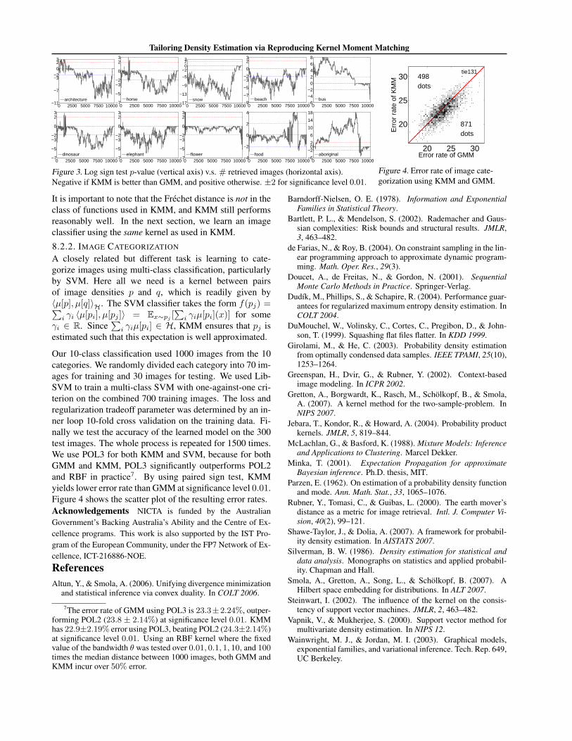
Settings In this experiment, the distance measure is fixedto EMD. We plug the densities estimated by GMM andKMM into EMD5, and compare the retrieval results. Para-meters for KMM and GMM were chosen in the same wayas in Section 7.4. Here KMM used POL3. For each image,we sampled 103 pixels and each pixel’s feature vector wasthe CIE-Lab value of a 5×5 window centered on it.Results We collected L = 10537 images from varioussources including FIRE and CIRES6. The dataset included10 labeled categories like horse, beach, and each cate-gory has 100 images. For each image Ic(i) from classc (c ∈ 1, ..., 10, i ∈ 1, ..., 100), we retrieved r(r ∈ 1, ..., L) closest images (in terms of EMD) fromthe whole database and counted how many among them arealso from class c, denoted as gc(i, r) for GMM and kc(i, r)for KMM. For each c and r, we performed a paired sign testbetween gc(i, r)100i=1 and kc(i, r)100i=1. Since p-value isalways in (0,1], we report in Figure 3 the log p-value if themedian of kc(i, r) − gc(i, r)100i=1 is higher than 0. Oth-erwise, we plot the negative log p-value. Negative valuesare in favor of KMM. In Figure 3, performance of KMM issuperior to or competitive with GMM in 8 categories andfor most values of r (number of retrieved images).

5EMD code from http://ai.stanford.edu/∼rubner/emd6FIRE: http://www-i6.informatik.rwth-aachen.de/

∼deselaers/fire.html, CIRES: http://cires.matthewriley.com

Tailoring Density Estimation via Reproducing Kernel Moment Matching

0 2500 5000 7500 10000−11

−7

−3−2

023

architecture0 2500 5000 7500 10000

−7

−5

−3−2

0

23

horse

0 2500 5000 7500 10000−17

−13

−9

−5

−2023

snow0 2500 5000 7500 10000

−9

−7

−5

−3−2

0

23

beach0 2500 5000 7500 10000

−6−4−2

02468

bus

0 2500 5000 7500 10000−7

−5

−3−2

0

23

dinosaur0 2500 5000 7500 10000

−7

−5

−3−2

0

23

elephant0 2500 5000 7500 10000

−7

−5

−3−2

0

23

flower0 2500 5000 7500 10000

−4

−2

0

2

4

food0 2500 5000 7500 10000

−6

−202

6

10

14

18

aboriginal

Figure 3. Log sign test p-value (vertical axis) v.s. # retrieved images (horizontal axis).Negative if KMM is better than GMM, and positive otherwise. ±2 for significance level 0.01.

20 25 30

20

25

30

Error rate of GMM

Err

or r

ate

of K

MM

871dots

498dots

tie131

Figure 4. Error rate of image cate-gorization using KMM and GMM.

It is important to note that the Frechet distance is not in theclass of functions used in KMM, and KMM still performsreasonably well. In the next section, we learn an imageclassifier using the same kernel as used in KMM.

8.2.2. IMAGE CATEGORIZATION

A closely related but different task is learning to cate-gorize images using multi-class classification, particularlyby SVM. Here all we need is a kernel between pairsof image densities p and q, which is readily given by〈µ[p], µ[q]〉H. The SVM classifier takes the form f(pj) =∑

i γi 〈µ[pi], µ[pj ]〉 = Ex∼pj[∑

i γiµ[pi](x)] for someγi ∈ R. Since

∑i γiµ[pi] ∈ H, KMM ensures that pj is

estimated such that this expectation is well approximated.

Our 10-class classification used 1000 images from the 10categories. We randomly divided each category into 70 im-ages for training and 30 images for testing. We used Lib-SVM to train a multi-class SVM with one-against-one cri-terion on the combined 700 training images. The loss andregularization tradeoff parameter was determined by an in-ner loop 10-fold cross validation on the training data. Fi-nally we test the accuracy of the learned model on the 300test images. The whole process is repeated for 1500 times.We use POL3 for both KMM and SVM, because for bothGMM and KMM, POL3 significantly outperforms POL2and RBF in practice7. By using paired sign test, KMMyields lower error rate than GMM at significance level 0.01.Figure 4 shows the scatter plot of the resulting error rates.Acknowledgements NICTA is funded by the AustralianGovernment’s Backing Australia’s Ability and the Centre of Ex-cellence programs. This work is also supported by the IST Pro-gram of the European Community, under the FP7 Network of Ex-cellence, ICT-216886-NOE.

ReferencesAltun, Y., & Smola, A. (2006). Unifying divergence minimization

and statistical inference via convex duality. In COLT 2006.

7The error rate of GMM using POL3 is 23.3±2.24%, outper-forming POL2 (23.8 ± 2.14%) at significance level 0.01. KMMhas 22.9±2.19% error using POL3, beating POL2 (24.3±2.14%)at significance level 0.01. Using an RBF kernel where the fixedvalue of the bandwidth θ was tested over 0.01, 0.1, 1, 10, and 100times the median distance between 1000 images, both GMM andKMM incur over 50% error.

Barndorff-Nielsen, O. E. (1978). Information and ExponentialFamilies in Statistical Theory.

Bartlett, P. L., & Mendelson, S. (2002). Rademacher and Gaus-sian complexities: Risk bounds and structural results. JMLR,3, 463–482.

de Farias, N., & Roy, B. (2004). On constraint sampling in the lin-ear programming approach to approximate dynamic program-ming. Math. Oper. Res., 29(3).

Doucet, A., de Freitas, N., & Gordon, N. (2001). SequentialMonte Carlo Methods in Practice. Springer-Verlag.

Dudık, M., Phillips, S., & Schapire, R. (2004). Performance guar-antees for regularized maximum entropy density estimation. InCOLT 2004.

DuMouchel, W., Volinsky, C., Cortes, C., Pregibon, D., & John-son, T. (1999). Squashing flat files flatter. In KDD 1999.

Girolami, M., & He, C. (2003). Probability density estimationfrom optimally condensed data samples. IEEE TPAMI, 25(10),1253–1264.

Greenspan, H., Dvir, G., & Rubner, Y. (2002). Context-basedimage modeling. In ICPR 2002.

Gretton, A., Borgwardt, K., Rasch, M., Scholkopf, B., & Smola,A. (2007). A kernel method for the two-sample-problem. InNIPS 2007.

Jebara, T., Kondor, R., & Howard, A. (2004). Probability productkernels. JMLR, 5, 819–844.

McLachlan, G., & Basford, K. (1988). Mixture Models: Inferenceand Applications to Clustering. Marcel Dekker.

Minka, T. (2001). Expectation Propagation for approximateBayesian inference. Ph.D. thesis, MIT.

Parzen, E. (1962). On estimation of a probability density functionand mode. Ann. Math. Stat., 33, 1065–1076.

Rubner, Y., Tomasi, C., & Guibas, L. (2000). The earth mover’sdistance as a metric for image retrieval. Intl. J. Computer Vi-sion, 40(2), 99–121.

Shawe-Taylor, J., & Dolia, A. (2007). A framework for probabil-ity density estimation. In AISTATS 2007.

Silverman, B. W. (1986). Density estimation for statistical anddata analysis. Monographs on statistics and applied probabil-ity. Chapman and Hall.

Smola, A., Gretton, A., Song, L., & Scholkopf, B. (2007). AHilbert space embedding for distributions. In ALT 2007.

Steinwart, I. (2002). The influence of the kernel on the consis-tency of support vector machines. JMLR, 2, 463–482.

Vapnik, V., & Mukherjee, S. (2000). Support vector method formultivariate density estimation. In NIPS 12.

Wainwright, M. J., & Jordan, M. I. (2003). Graphical models,exponential families, and variational inference. Tech. Rep. 649,UC Berkeley.