Talk III: The h-principle for isometric embeddings

Vincent Borrelli

August 30, 2012

1 From the Convex Integration Theory to the Nash-Kuiper Theorem

The goal of this text is to recover the Nash-Kuiper result on C1 isometricembeddings from the machinery of the Gromov Integration Theory.

Theorem (Nash 54, Kuiper 55).– Let Mn be a compact1 Rieman-

nian manifold and f0 : (Mn, g)C1

−→ Eq be a strictly short embedding (i.e∆ := g − f∗0 〈·, ·〉Eq is a Riemannian metric). Then, for every ε > 0, thereexists a C1 isometric embedding f : (Mn, g) −→ Eq such that ‖f−f0‖C0 ≤ ε.

Nevertheless, there are three major obstacles to apply the Gromov Theoremfor Ample relations here. First, the isometric relation is closed, second, it isnot ample, third the convex integration process produces non-injective mapsin general. We have seen previously that the first obstacle can be circum-vented by iteratively applying the Gromov Theorem. But to deal with thetwo other obtacles, we will have to adapt the Gromov machinery. Let us seewhy.

Assume, for a practical presentation, that our manifold M is a Riemanniansquare ([0, 1]2, g) where g is any metric and that q = 3. Our goal is toproduce a map f : ([0, 1]2, g) −→ E3 which is ε-isometric for a given ε > 0.Thus, our 1-jet space is

J1([0, 1]2,E3) = [0, 1]2 × E3 × (E3)2

and our (open) differential relation Rε is

Rε = {(c, y, v1, v2) | gij(c)− ε ≤ 〈vi, vj〉 ≤ gij(c) + ε, 1 ≤ i, j ≤ 2}.1This compactness hypothesis is not essential but it will help simplifying the exposition.

1

Let f0 : ([0, 1]2, g) −→ E3 be a strictly short map. To apply the Gromovmachinery for ample relations we need to extend it to a section σ of ourdifferential relation Rε

σ : [0, 1]2 −→ Rε ⊂ J1([0, 1]2,E3)c = (c1, c2) 7−→ (c, f0(c), v1(c), v2(c)).

Since the topology of the base manifold is trivial, finding such a section iseasy. In fact, there is a considerable latitude for the choice of (v1, v2) sincethe constraints are underdetermined : v1(c) and v2(c) must be of lengthapproximatively

√g11(c) and

√g22(c) and the angle between then is ap-

proximatively α = arccos

(g12(c)√

g11(c)√g22(c)

).

The first step of the machinery is to perform a convex integration in thedirection of the c2 variable. We denote by p⊥2 the projection

(c, y, v1, v2) 7−→ (c, y, v1)

and we set R⊥2z = Rε ∩ (p⊥2)−1(z) for every z = (c, y, v1). The space R⊥2

z

is a thickening of a circle.

The space R⊥2z in E3. The angle of the cone with basis R⊥2

z is approximatively α.

We have denoted v for ∂f0∂c2

(c).

Even if f0 is strictly short, there is no reason why the vector∂f0∂c2

(c) should

be in the convex hull of R⊥2

z(c) with z(c) = (c, f0(c), v1(c)), c ∈ [0, 1]2. Notealso that the natural choice

v1(c) :=√g11(c)

∂f0∂c1

(c)

‖∂f0∂c1(c)‖

2

is of no help since∂f0∂c2

(c) will then lies in the convex hull of the cone with

basis R⊥2

z(c) but not in the convex hull of R⊥2

z(c) in general. In short, a directapplication of the Gromov Theorem for Ample Relations fails.

2 A strategy to solve the relation of isometric maps

Recall that we already have found a strategy to solve the closed relation ofisometric maps R by iteratively solving a sequence (R̃k)k∈N∗ of open differ-ential relations converging toward R.

Let ∆ := g − f∗0 〈·, ·〉Eq and (δk)k∈N∗ be a strictly increasing sequence ofpositive numbers converging toward 1. We set

gk := f∗0 〈·, ·〉Eq + δk∆.

Obviously (gk)k∈N∗ ↑ g. The relation Rk is defined to be the relation ofgk-isometric maps and R̃k is a thickning of Rk. The strategy is to startwith the strictly short map f0, then to solve R̃1 to get a new map f1 whichis strictly short for R̃2, then to solve R̃2, etc. Let fk−1 be a strictly shortembedding for gk−1, the fundamental step is thus to build a new map fksuch that

1) fk is a solution of R̃k,2) fk is C0-close to fk−1,3) ‖fk − fk−1‖C1 is under control,4) fk is an embedding.

Note that since the sequence of metrics (gk)k∈N∗ is strictly increasing, allthe Rk are disjoint. Thus, provided the thickning R̃k is small enough, themap fk will be short for gk+1.

In what follows we describe how to buid such a map fk from fk−1 since,as we have just seen, we can not apply directly the Gromov Theorem forAmple Relations.

3 How to adapt the Gromov machinery

For simplicity, we first assume that Mn is the cube [0, 1]n. The metric dis-torsion induced by fk−1 is measured by a field of bilinear forms obtained as

3

the difference∆k := gk − f∗k−1〈., .〉Eq .

This difference is a metric since fk−1 is strictly short, thus the image of themap

∆k : Mn −→M ⊂ (En ⊗ En)∗

lies inside the positive cone M of inner products of En. There exist Sk ≥n(n+1)

2 linear forms `k,1, . . . `k,Skof En such that

gk − f∗k−1〈., .〉Eq =

Sk∑j=1

ρk,j`k,j ⊗ `k,j

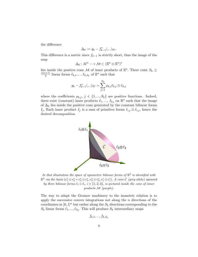
where the coefficients ρk,j , j ∈ {1, ..., Sk} are positive functions. Indeed,there exist (constant) inner products I1, ..., ILk

on Rn such that the imageof ∆k lies inside the positive cone generated by the constant bilinear formsIj . Each inner product Ij is a sum of primitive forms `i,j ⊗ `i,j , hence thedesired decomposition.

In that illustration the space of symmetric bilinear forms of R3 is identified with

R3 via the basis (e∗1 ⊗ e∗2 + e∗2 ⊗ e∗1, e∗2 ⊗ e∗2, e∗1 ⊗ e∗1). A cone C (grey-white) spanned

by three bilinear forms `i ⊗ `i, i ∈ {1, 2, 3}, is pictured inside the cone of inner

products M (purple).

The way to adapt the Gromov machinery to the isometric relation is toapply the successive convex integrations not along the n directions of thecoordinates in [0, 1]n but rather along the Sk directions corresponding to theSk linear forms `1, ..., `Sk

. This will produce Sk intermediary maps

fk,1, ..., fk,Sk

4

such that

gk − f∗k,1〈., .〉Eq ≈ ρk,2`k,2 ⊗ `k,2+ρk,3`k,3 ⊗ `k,3+...+ρk,Sk`k,Sk

⊗ `k,Sk

gk − f∗k,2〈., .〉Eq ≈ ρk,3`k,3 ⊗ `k,3+...+ρk,Sk`k,Sk

⊗ `k,Sk

......

gk − f∗k,Sk−1〈., .〉Eq ≈ ρk,Sk`k,Sk

⊗ `k,Sk

gk − f∗k,Sk〈., .〉Eq ≈ 0.

In orther words, the isometric default ∆k is going to be reduced step bystep by a succession of convex integrations that detroy the coefficients inthe decomposition one by one. The map fk := fk,Sk

is then a solution of

R̃k.

Note that

f∗k,j〈., .〉Eq − f∗k,j−1〈., .〉Eq = (gk − f∗k,j−1〈., .〉Eq)− (gk − f∗k,j〈., .〉Eq)

≈ ρk,j`k,j ⊗ `k,j .

Hence, in that new approach, the fundamental problem is the following :

Fundamental problem.– Given a positive function ρ, a linear form ` 6= 0and an embedding f0 how to build an other embedding f such that

f∗〈., .〉Eq ≈ µ

where µ := f∗0 〈., .〉Eq + ρ `⊗ ` ?

We are going to solve this problem thanks to a convex integration processdescribed below.

4 The one dimensional case

In the above fundamental problem, the embedding f0 is isometric in thedirections lying inside ker ` and short in the directions transverse to ker `.We redress this defect by elongating f0 in a direction transverse to ker `. Theelongation is generated by a normal deformation which gives to the imagesubmanifold a corrugated shape.

5

A plane and a corrugated plane.

One difficulty in the construction of f rests in the choice of a good transversaldirection to perform the convex integration process. This difficulty obviouslyvanishes in the case n = 1, that is why we begin by considering this case first.

One dimensional fundamental problem.– Let f0 : [0, 1] −→ Eq be anembedding, ρ a positive function, ` 6= 0 a linear form on R, how to build another embedding f such that

∀c ∈ [0, 1], ‖f ′(c)‖2 ≈ ‖f ′0(c)‖2 + ρ(c)`2(∂c) ?

Of course that one dimensional problem is trivial, even if the approxima-tion symbol (≈) is replaced by a true equality (=). But the interest lieselsewhere: the convex integration theory offers a way to solve that problemthat can be generalized to any dimension.

Note that the differential relation S of that problem depends on the pointc ∈ [0, 1], precisely

S = {(c, y, v1) | ‖v1‖ = r(c)} ⊂ J1([0, 1],Rq)

where r(c) :=√‖f ′0(c)‖2 + ρ(c)`2(∂c). We thus have to find a family of loops

(hc)c∈[0,1]:

hc : [0, 1] −→ Sq−1(r(c)) ⊂ Eq

such that

f ′0(c) =

∫ 1

0hc(s)ds.

Let n : [0, 1] −→ Eq a unit normal to the curve f0. We set

hc(s) := r(c)eiα(c) cos 2πs

6

where eiθ := cos θ t + sin θ n and t :=f ′0‖f ′0‖

. It is easily checked that∫ 1

0r(c)eiα(c) cos 2πsds = r(c)J0(α(c)) t(c)

where J0 is the Bessel function of order 0. We thus have to choose

α(c) := J−10

(‖f ′0(c)‖r(c)

)(recall that J0 is invertible on [0, κ] where κ ≈ 2.4 is the smallest positiveroot of J0).

The loop hc.

We now define f by the following one dimensional convex integrationformula:

f(c) := f0(0) +

∫ c

0r(u)eiα(u) cos 2πNu du.

with N ∈ N∗.

Observation.– We call N the number of corrugations of the convex inte-gration formula.

Lemma.– The map f solves the one dimensional fundamental problem. Itsspeed ‖f ′‖ is equal to the given function r = (‖f ′0‖2 + ρ`2(∂c))

12 . Moreover

‖f − f0‖C0 = O(1N

)and if N is large enough f is an embedding.

Proof.– The relation ‖f ′‖2 = ‖f ′0‖2 + ρ`2(∂c) ensues from the very defini-tion of f. If N is large enough, the image of f lies inside a small tubularneighborhood of f0. Since f is a normal deformation of f0, it is embedded.�.

7

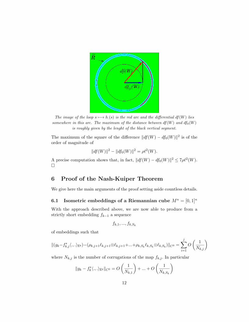
A short curve f0 (black) and the curve f obtained with the one dimensional

convex integration formula (grey, N = 9 and N = 20).

5 A Kuiper-like convex integration process

5.1 A first attempt

We now come back to the n-dimensional case and we assume for simplicitythat ker ` = Span(e2, ..., en) and `(e1) = 1 where (e1, ..., en) is the stan-dard basis of [0, 1]n. The previous convex integration formula can be easilygeneralized to the n-dimensional case by setting:

f(s, c) := f0(0, c) +

∫ s

0r(u, c)eiα(u,c) cos 2πNu du

with s ∈ [0, 1], c = (c2, ..., cn) ∈ [0, 1]n−1, N ∈ N∗, r =√µ(e1, e1) =√

‖f ′0‖2 + ρ, α = J−10

(‖df0(e1)‖

r

), eiθ = cos θ t + sin θ n, t = df0(e1)

‖df0(e1)‖ and n

is any unit normal to f0.

But surprisingly the resulting map f does not solve the fundamentalproblem. Let us see why. The isometric relation

f∗〈., .〉Eq = f∗0 〈., .〉Eq + ρ `⊗ `

8

is equivalent to the following system of equations:

〈df(e1), df(e1)〉Eq = 〈df0(e1), df0(e1)〉Eq + ρ〈df(e1), df(ej)〉Eq = 〈df0(e1), df0(ej)〉Eq if j 6= 1〈df(ei), df(ej)〉Eq = 〈df0(ei), df0(ej)〉Eq with i > 1 and j > 1.

In the one hand we have

∂f

∂s(s, c) = r(s, c)eiα(s,c) cos 2πNs

thus ‖df(e1)‖2 = r2(s, c) and the first equation is fulfilled. In the other

hand, the C1,1̂ closeness of f to f0:

‖f − f0‖C1,1̂ = O

(1

N

)implies that ‖df(ej)− df0(ej)‖ = O

(1N

)for every j 6= 1. In particular

〈df(ei), df(ej)〉Eq = 〈df0(ei), df0(ej)〉Eq +O

(1

N

)for every i > 1, j > 1. The problem arises with the mixted term 〈df(e1), df(ej)〉Eq ,j > 1. Indeed

〈df(e1), df(ej)〉Eq = 〈df(e1), df0(ej)〉Eq +O(1N

)= 〈r(s, c)eiα(s,c) cos 2πNs, df0(ej)〉Eq +O

(1N

)= 〈r(s, c) cos(α(s, c) cos 2πNs)t, df0(ej)〉Eq +O

(1N

)= r(s,c)

‖df0(e1)‖ cos(α(s, c) cos 2πNs)〈df0(e1), df0(ej)〉Eq +O(1N

)Thus, unless µ(e1, ej) = 〈df0(e1), df0(ej)〉Eq is null, there is no reason why〈df(e1), df(ej)〉Eq should be equal to 〈df0(e1), df0(ej)〉Eq .

5.2 Adjusting the convex integration formula

To correct this default we need to adjust our convex integration formula:rather than performing the normal deformation along straight lines we aregoing to follow the integral lines of some well chosen vector field. Let

W (s, c) := e1 +

n∑j=2

ζj(s, c)ej

9

be a vector field µ-orthogonal to ker `, that is µ(W, ej) = 0 for j ∈ {2, ..., n}.Let s 7→ ϕ(s, c) be the integral curve of W issuing from (0, c) that is

∂ϕ

∂s(s, c) = W (ϕ(s, c)) and ϕ(0, c) = (0, c).

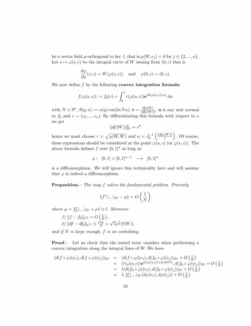
We now define f by the following convex integration formula:

f(ϕ(s, c)) := f0(c) +

∫ s

0r(ϕ(u, c))eiθ(ϕ(u,c)),u) du

with N ∈ N∗, θ(q, u) := α(q) cos(2πNu), t = df0(W )‖df0(W )‖ , n is any unit normal

to f0 and c = (c2, ..., cn). By differentiating this formula with respect to swe get

‖df(W )‖2Eq = r2

hence we must choose r =√µ(W,W ) and α = J−10

(‖df0(W )‖

r

). Of course,

these expressions should be considered at the point ϕ(u, c) (or ϕ(s, c)). Theabove formula defines f over [0, 1]n as long as

ϕ : [0, 1]× [0, 1]n−1 −→ [0, 1]n

is a diffeomorphism. We will ignore this technicality here and will assumethat ϕ is indeed a diffeomorphism.

Proposition.– The map f solves the fundamental problem. Precisely

‖f∗〈., .〉Eq − µ‖ = O

(1

N

)where µ = f∗0 〈., .〉Eq + ρ `⊗ `. Moreover

1) ‖f − f0‖C0 = O(1N

),

2) ‖df − df0‖C0 ≤ CteN +

√7ρ

12 |`(W )|,

and if N is large enough, f is an embedding.

Proof.– Let us check that the mixed term vanishes when performing aconvex integration along the integral lines of W. We have

〈d(f ◦ ϕ)(e1), d(f ◦ ϕ)(ej)〉Eq = 〈d(f ◦ ϕ)(e1), d(f0 ◦ ϕ)(ej)〉Eq +O(1N

)= 〈r(ϕ(s, c))eiα(ϕ(s,c)) cos 2πNs, d(f0 ◦ ϕ)(ej)〉Eq +O

(1N

)= λ〈d(f0 ◦ ϕ)(e1), d(f0 ◦ ϕ)(ej)〉Eq +O

(1N

)= λ f∗0 〈., .〉Eq(dϕ(e1), dϕ(ej)) +O

(1N

)10

where λ = r(ϕ(s,c))‖d(f0◦ϕ)(e1)‖ cos(α(ϕ(s, c)) cos 2πNs). From the definition of W

we deduce that ϕ(s, c) = se1 + ψ(s, c) with ψ(s, c) ∈ ker `. Therefore

∀ j ∈ {2, ..., n}, dϕ(ej) ∈ ker `.

In particular

f∗0 〈., .〉Eq(dϕ(e1), dϕ(ej)) = µ(dϕ(ej), dϕ(e1))

and since dϕ(e1) = W which is µ-orthogonal to ker ` we have

µ(dϕ(ej), dϕ(e1)) = 0.

As a consequence 〈d(f ◦ ϕ)(e1), d(f ◦ ϕ)(ej)〉Eq = O(1N

)and

‖(f ◦ ϕ)∗〈., .〉Eq(e1, ej)− (ϕ∗µ)(e1, ej)‖ = O

(1

N

)for j ∈ {2, ..., n}. It is straightforward to check that

‖(f ◦ ϕ)∗〈., .〉Eq(ei, ej)− (ϕ∗µ)(ei, ej)‖ = O

(1

N

)for i > 1, j > 1 and the equality ‖df(W )‖2Eq = r2 means that

‖(f ◦ ϕ)∗〈., .〉Eq(e1, e1)− (ϕ∗µ)(e1, e1)‖ = 0.

Therefore

‖(f ◦ ϕ)∗〈., .〉Eq − ϕ∗µ‖ = O

(1

N

)and since [0, 1]n is compact

‖f∗〈., .〉Eq − µ‖ = O

(1

N

).

The general theory of convex integration ensures that ‖f−f0‖C1,1̂ = O(1N

).

This proves point 1 and reduces point 2 to the proof of the following inequal-ity:

‖df(W )− df0(W )‖C0 ≤√

7ρ12 |`(W )|.

The maximum of distance between df(W ) and df0(W ) could be roughlyestimated by using the Pythagorean Theorem (see the figure below).

11

The image of the loop s 7−→ h.(s) is the red arc and the differential df(W ) lies

somewhere in this arc. The maximum of the distance between df(W ) and df0(W )

is roughly given by the lenght of the black vertical segment.

The maximum of the square of the difference ‖df(W ) − df0(W )‖2 is of theorder of magnitude of

‖df(W )‖2 − ‖df0(W )‖2 = ρ`2(W ).

A precise computation shows that, in fact, ‖df(W )− df0(W )‖2 ≤ 7ρ`2(W ).�

6 Proof of the Nash-Kuiper Theorem

We give here the main arguments of the proof setting aside countless details.

6.1 Isometric embeddings of a Riemannian cube Mn = [0, 1]n

With the approach described above, we are now able to produce from astrictly short embedding fk−1 a sequence

fk,1, ..., fk,Sk

of embeddings such that

‖(gk−f∗k,j〈., .〉Eq)−(ρk,j+1`k,j+1⊗`k,j+1+...+ρk,Sk`k,Sk⊗`k,Sk

)‖C0 =

j∑i=1

O

(1

Nk,j

)where Nk,j is the number of corrugations of the map fk,j . In particular

‖gk − f∗k 〈., .〉Eq‖C0 = O

(1

Nk,1

)+ ...+O

(1

Nk,Sk

)12

where we have set fk := fk,Sk. Since gk < gk+1, the embedding fk,j is strictly

short for gk+1 if∑j

i=1O(

1Nk,j

)is small enough.

By iterating the process, we generate an infinite sequence of embeddings

f0, f1,1, ..., f1,S1 =: f1, f2,1, ..., f2,S2 =: f2, etc.

Since

‖fk − fk−1‖C0 = O

(1

Nk,1

)+ ...+O

(1

Nk,Sk

)this sequence will converge C0 if we choose the Nk,js large enough. Letf∞ the limit map. The crucial point is that the sequence (fk)k∈N is alsoC1-converging. Indeed we have

‖dfk − dfk−1‖C0 ≤Sk∑j=1

O

(1

Nk,j

)+√

7

Sk∑j=1

ρ12k,j |`k,j(Wk,j)|.

Let us assume that the `k,js and the Wk,js are normalized by requiring, forinstance, that `k,j(.) = 〈Uk,j , .〉En with ‖Uk,j‖En = 1 and Wk,j = Uk,j + Vk,jwith Vk,j ∈ ker `k,j . From the decomposition

gk − f∗k−1〈., .〉Eq =

Sk∑j=1

ρk,j`k,j ⊗ `k,j

we deduce that there exists a constant K(`1, ..., `Sk) > 0 depending on the

chosen `1, ..., `Sksuch that

√7∑Sk

j=1 ρ12k,j |`j(Wk,j)| ≤ K(`1, ..., `Sk

)‖gk − f∗k−1〈., .〉Eq‖.

But we also have

‖gk−1 − f∗k−1〈., .〉Eq‖ =

Sk−1∑j=1

O

(1

Nk−1,j

),

hence

√7∑Sk

j=1 ρ12k,j |`j(Wk,j)| ≤ K(`1, ..., `Sk

)‖gk − gk−1‖+∑Sk−1

j=1 O(

1Nk−1,j

)≤ K(`1, ..., `Sk

)√δk − δk−1‖∆‖+

∑Sk−1

j=1 O(

1Nk−1,j

).

13

In fact, since Mn = [0, 1]n is compact, one can choose a stationnary sequenceof set of linear forms {`k,1, ..., `k,Sk

} so that it is stationnary. In particular,there exists a uniform upper bound K for all the constants K(`1, ..., `Sk

).Thus

‖dfk − dfk−1‖C0 ≤ K√δk − δk−1‖∆‖+

Sk−1∑j=1

O

(1

Nk−1,j

).

The sequence (fk)k∈N can be made C1-converging by choosing the sequence(δk)k∈N∗ such that ∑√

δk − δk−1 < +∞.

For instance, δk = 1− e−kγ with γ > 0 is appropriate.

Once the sequence is C1-converging, it is then straightforward to see thatthe limite is an isometry. Indeed from

gk−1 < f∗k 〈., .〉Eq < gk+1

we deduce by taking the limite that

limk−→∞

(f∗k 〈., .〉Eq) = g.

From the C1-convergence we have

limk−→∞

(f∗k 〈., .〉Eq) = ( limk−→∞

fk)∗〈., .〉Eq

therefore f∗∞〈., .〉Eq = g. Note that f∞ is necessarily an C1 immersion.

The fact that f∞ is an embedding is easily obtained in the codimension onecase. Indeed, f∞ is C0 close to a C1 embedding fk and is such that thetangent planes to f∞ are C0-close to the corresponding tangent planes offk. In codimension one, this implies that f∞ is an embedding. In greatercodimension, the argument is more involved, see [3], p. 393-394.

6.2 Isometric embeddings of a compact manifold

It is enough to perform a cubical decomposition of the manifold and thento glue the local solutions together with the help of the following relativeversion of the proof of the Nash-Kuiper theorem for the cube:

14

Isometric embedding of the cube: relative version .– Let ([0, 1]n, g)

be a Riemannian cube, A ⊂ [0, 1]n be a polyhedron2, f0 : ([0, 1]n, g)C1

−→ Eqbe an embedding which is isometric over an open neighbourhood Op A ofA and is strictly short elsewhere. Then, for every ε > 0, there exists a C1

isometric embedding f : ([0, 1]n, g) −→ Eq such that ‖f − f0‖C0 ≤ ε andf = f0 over a smaller neighbourhood Op1 A.

References

[1] Y. Eliahsberg et N. Mishachev, Introduction to the h-principle,Graduate Studies in Mathematics, vol. 48, A. M. S., Providence, 2002.

[2] N. Kuiper, On C1-isometric imbeddings I, II, Indag. Math. 17 (1955),545-556, 683-689.

[3] F. Nash, C1-isometric imbeddings, Ann. Math. 63 (1954), 384-396.

2That is a subcomplex of a certain smooth triangulation of [0, 1]n.

15