Tankvision Tank Scanner NXA820, Data Concentrator NXA821 ... · Tank Scanner NXA820, Data...

BA00426G/00/EN/01.12

71193832

Valid as of software version:

V01.04

Operating Instructions

Tankvision

Tank Scanner NXA820, Data Concentrator

NXA821, Host Link NXA822

System Description

Table of Contents

3

Table of Contents

1 Target audience for this manual . . . . . . 4

2 Version history . . . . . . . . . . . . . . . . . . . 4

3 Application . . . . . . . . . . . . . . . . . . . . . . 4

3.1 Inventory control . . . . . . . . . . . . . . . . . . . . . . . . . . 4

3.2 Application areas . . . . . . . . . . . . . . . . . . . . . . . . . . . 4

4 Explanation of signs an abbreviations . 5

5 Identifying the components . . . . . . . . . 6

5.1 Nameplate . . . . . . . . . . . . . . . . . . . . . . . . . . . . . . . 6

5.2 Tank Scanner NXA820 . . . . . . . . . . . . . . . . . . . . . . 7

5.3 Data Concentrator NXA821 . . . . . . . . . . . . . . . . . . 8

5.4 Host Link NXA822 . . . . . . . . . . . . . . . . . . . . . . . . . 9

5.5 Explosion picture . . . . . . . . . . . . . . . . . . . . . . . . . 10

5.6 Tankvision OPC Server . . . . . . . . . . . . . . . . . . . . . 10

5.7 Tankvision Printer Agent . . . . . . . . . . . . . . . . . . . . 10

5.8 Tankvision Alarm Agent . . . . . . . . . . . . . . . . . . . . 11

6 PC recommendations . . . . . . . . . . . . . 12

6.1 PC connection for viewing data . . . . . . . . . . . . . . . 12

6.2 Recommendations when using OPC Server,

Printer Agent or Alarm Agent . . . . . . . . . . . . . . . . 12

6.3 Alternations from the recommendations . . . . . . . . . 12

7 Connections to gauges and

host systems. . . . . . . . . . . . . . . . . . . . 13

7.1 Field instruments and slave devices . . . . . . . . . . . . 13

7.2 Host Systems communication . . . . . . . . . . . . . . . . 17

8 Examples . . . . . . . . . . . . . . . . . . . . . . 18

8.1 System architecture . . . . . . . . . . . . . . . . . . . . . . . . 18

8.2 Screen examples in Browser . . . . . . . . . . . . . . . . . 19

9 Calculations . . . . . . . . . . . . . . . . . . . . 21

9.1 API Flow Charts . . . . . . . . . . . . . . . . . . . . . . . . . . 21

9.2 GBT calculation flow chart . . . . . . . . . . . . . . . . . . 34

9.3 Mass Measurement . . . . . . . . . . . . . . . . . . . . . . . . 40

9.4 Calculations for liquefied gases . . . . . . . . . . . . . . . 42

9.5 CTSh . . . . . . . . . . . . . . . . . . . . . . . . . . . . . . . . . . 45

9.6 Alcohol calculations . . . . . . . . . . . . . . . . . . . . . . . . 49

9.7 Annex A.1

. . . . . . . . . . . . . . . . . . . . . . . . . . . . . . . . . . . . . . . 51

9.8 Annex A.2 . . . . . . . . . . . . . . . . . . . . . . . . . . . . . . 53

9.9 Annex A.3 . . . . . . . . . . . . . . . . . . . . . . . . . . . . . . 54

9.10 Annex A.4 . . . . . . . . . . . . . . . . . . . . . . . . . . . . . . 55

9.11 Documentation . . . . . . . . . . . . . . . . . . . . . . . . . . . 55

Target audience for this manual

4

1 Target audience for this manual

This manual is giving detailed information on the system capabilities and architecture. It supports

project and sales engineers in designing the system architecture during acquisition and execution

phase. Furthermore during operation time of the system all servicing personnel in need of detailed

knowledge about the system capabilites.

2 Version history

3 Application

3.1 Inventory control

By using Tankvision to monitor the tank level and stored volume of valuable liquids remotely,

owners or operators of tank farms or terminals for petroleum products and chemicals (liquids) can

visualize the volumes or mass of the stored medium in real time. The data can be used to plan the

inventory and distribution. The data can also be used to manage tank farm operations like pumping

or transferring products.

Tankvision has its unique concept using network technology. Without using proprietary software,

the users can visualize and manage their valuable liquids stored in the tanks by a web browser.

Tankvision is a flexible and cost effective solution due to its scalable architecture. The application

coverage goes from small depots with only a few tanks up to refineries.

3.2 Application areas

• Tank farms in refineries

• Ship loading terminals

• Marketing and distribution terminals

• Pipeline terminals

• Logistic terminals for tanks storing products like crude oils, refined white and black products,

chemicals, LPGs, fuels, biofuels, alcohols

Document version Valid for SW version Changes to the previous version

BA00426G/00/EN/01.12 01.02.02-00xxx/01.04.00 Initial version

Explanation of signs an abbreviations

5

4 Explanation of signs an abbreviations

In order to highlight safety-relevant or alternative operating procedures in the manual, the following

conventions have been used, each indicated by a corresponding symbol in the margin.

Safety conventions

#Warning!

A warning highlights actions or procedures which, if not performed correctly, will lead to personal

injury, a safety hazard or destruction of the device.

"Caution!

Caution highlights actions or procedures which, if not performed correctly, may lead to personal injury

or incorrect functioning of the device.

!Note!

A note highlights actions or procedures which, if not performed correctly, may indirectly affect

operation or may lead to an device response which is not planned.

Explosion protection

0Device certified for use in explosion hazardous area

If the device has this symbol embossed on its name plate it can be installed in an explosion hazardous

area.

-Explosion hazardous area

Symbol used in drawings to indicate explosion hazardous areas. Devices located in and wiring entering

areas with the designation "explosion hazardous areas" must conform with the stated type of protection.

.Safe area (non-explosion hazardous area)

Symbol used in drawings to indicate, if necessary, non-explosion hazardous areas. Devices located in

safe areas still require a certificate if their outputs run into explosion hazardous areas.

Electrical symbols

% Direct voltage

A terminal to which or from which a direct current or voltage may be applied or supplied.

&Alternating voltage

A terminal to which or from which an alternating (sine-wave) current or voltage may be applied or

supplied.

)Grounded terminal

A grounded terminal, which as far as the operator is concerned, is already grounded by means of an

earth grounding system.

*Protective grounding (earth) terminal

A terminal which must be connected to earth ground prior to making any other connection to the

equipment.

+Equipotential connection (earth bonding)

A connection made to the plant grounding system which may be of type e.g. neutral star or

equipotential line according to national or company practice.

Temperature resistance of the connection cables

States, that the connection cables must be resistant to a temperature of at least 85 °C (185 °F).t >85°C

Identifying the components

6

5 Identifying the components

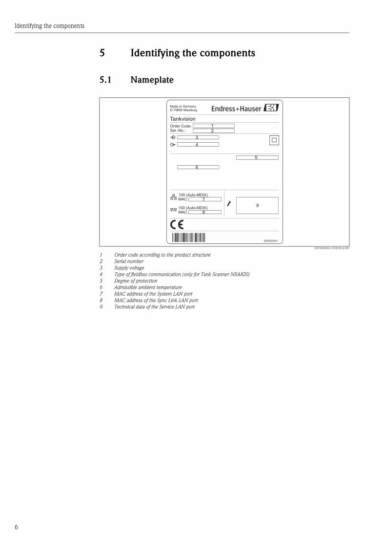
5.1 Nameplate

L00-NXA82xxx-18-00-00-yy-001

1 Order code according to the product structure

2 Serial number

3 Supply voltage

4 Type of fieldbus communication (only for Tank Scanner NXA820)

5 Degree of protection

6 Admissible ambient temperature

7 MAC address of the System LAN port

8 MAC address of the Sync Link LAN port

9 Technical data of the Service LAN port

Made in GermanyD-79689 Maulburg

Tankvision

Order Code:Ser.-No.:

250002393--

100 (Auto-MDIX)MAC:

100 (Auto-MDIX)MAC:

12

3

4

5

6

7

8

9


7

5.2 Tank Scanner NXA820

• The Tank Scanner NXA820 connects multiple tank gauges:

from up to 15 tanks via one field-loop. The Tank Scanner NXA820 supports different field

protocols (Modbus EIA485, Sakura V1, Whessoe WM550).

• The measured values are transmitted by the network and visualized on HTML pages.

• The Tank Scanner NXA820 can be used stand-alone for small tank farms, but also be integrated

into a large system for use in refineries.

• The Tank Scanner NXA820 is equipped with a full set of tank inventory calculations. The

calculations are based on various international standards such as API, ASTM, IP and many others.

Measured values are used to calculate volume and mass.

5.2.1 Ordering information

Detailed ordering information is available from the following sources:

• In the Product Configuration on the Endress+Hauser website: www.endress.com ? Select country

? Instruments ? Select device ? Product page function: Configure this product

• From your Endress+Hauser Sales Center: www.endress.com/worldwide

! Note!

Product Configurator - the tool for individual product configuration

• Up-to-the-minute configuration data

• Depending on the device: Direct input of measuring point-specific information such as measuring

range or operating language

• Automatic verification of exclusion criteria

• Automatic creation of the order code and its breakdown in PDF or Excel output format

• Ability to order directly in the Endress+Hauser Online Shop

5.2.2 Product picture

L00-NXA8xxxx-10-08-06-xx-002


8

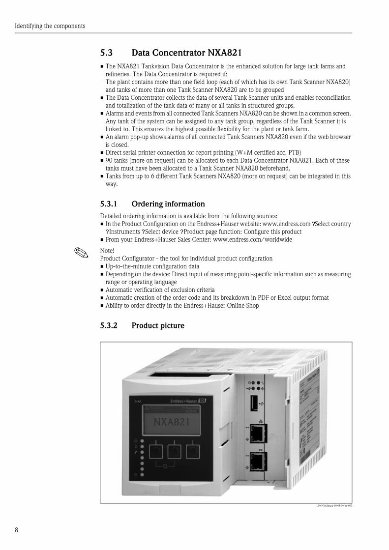
5.3 Data Concentrator NXA821

• The NXA821 Tankvision Data Concentrator is the enhanced solution for large tank farms and

refineries. The Data Concentrator is required if:

The plant contains more than one field loop (each of which has its own Tank Scanner NXA820)

and tanks of more than one Tank Scanner NXA820 are to be grouped

• The Data Concentrator collects the data of several Tank Scanner units and enables reconciliation

and totalization of the tank data of many or all tanks in structured groups.

• Alarms and events from all connected Tank Scanners NXA820 can be shown in a common screen.

Any tank of the system can be assigned to any tank group, regardless of the Tank Scanner it is

linked to. This ensures the highest possible flexibility for the plant or tank farm.

• An alarm pop-up shows alarms of all connected Tank Scanners NXA820 even if the web browser

is closed.

• Direct serial printer connection for report printing (W+M certified acc. PTB)

• 90 tanks (more on request) can be allocated to each Data Concentrator NXA821. Each of these

tanks must have been allocated to a Tank Scanner NXA820 beforehand.

• Tanks from up to 6 different Tank Scanners NXA820 (more on request) can be integrated in this

way.






! Note!









L00-NXA8xxxx-10-08-06-xx-003


9

5.4 Host Link NXA822

• The Host Link NXA822 collects data from all Tank Scanners NXA820 on a network and transfers

them to the host system.

• The MODBUS option supports serial EIA-232(RS) and EIA-485(RS) or MODBUS TCP/IP. The

NXA822 is configured as a MODBUS slave. Supported functions are:

– Coil Status (#01)

– Holding Registers (#03)

– Input Registers (#04)

– Write Modbus Values (#06)

• The MODBUS register map is described via XML files and can easily be adapted to individual

MODBUS master requirements.

• Gauge commands for Servo Gauges

• 90 tanks (more on request) can be allocated to each Host Link NXA822. Each of these tanks must

have been allocated to a Tank Scanner NXA820 beforehand.

• Tanks from up to 6 different Tank Scanners NXA820 (more on request) can be integrated in this

way.

• Per system 2 NXA822 units can be installed.






! Note!









L00-NXA8xxxx-10-08-06-xx-004


10

5.5 Explosion picture

L00-NXA82xxx-16-00-00-xx-071

1 Cover plate

2 Inner electronics

3 Housing

5.6 Tankvision OPC Server

• The OPC Server is a Windows program installed on a PC connecting to NXA820 and allows

access to measured and calculated tank parameters.

• The OPC Server connects to OPC clients on the same PC or other PCs via LAN.

• The OPC Server supports browsing tanks and tank parameters on NXA820.

• The OPC Server is included in each NXA820 and can be uploaded to the PC.

• The OPC Server is based on OPC DA V2.05a

5.7 Tankvision Printer Agent

• The Printer Agent is a Windows program installed on a PC, connecting to NXA820/NXA821.

• The program is running in the background and enables (scheduled) printing reports on connected

printers.

• Up to 3 printers (directly connected to the PC or network printers) can be assigned to the Printer

Agent.

• If a printout can not be performed, a record is kept within the Printer Agent.

• The printer agent software is included in each NXA820 and can be uploaded to the PC.

1

2

3


11

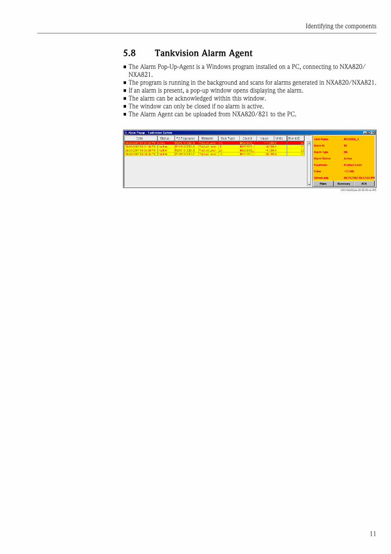
5.8 Tankvision Alarm Agent

• The Alarm Pop-Up-Agent is a Windows program installed on a PC, connecting to NXA820/

NXA821.

• The program is running in the background and scans for alarms generated in NXA820/NXA821.

• If an alarm is present, a pop-up window opens displaying the alarm.

• The alarm can be acknowledged within this window.

• The window can only be closed if no alarm is active.

• The Alarm Agent can be uploaded from NXA820/821 to the PC.

L00-NXA82xxx-20-00-00-en-005

PC recommendations

12

6 PC recommendations

6.1 PC connection for viewing data

Tankvision Tank Scanner NXA820, Tankvision Data Concentrator NXA821 and Tankvision Host

Link NXA822 are providing a web server to view and enter data or perform configurations. Viewing

the pages requires a web browser and JAVA runtime installed on a PC.

PC and the Tankvision components must be connected within the same Local Area Network (LAN)

consisting out of Ethernet lines, switches and/or routers.

! Note!

HUBs shall not be used. In secured systems e.g. for W&M purposes, routers cannot be used. If

company policies allow a remote connection into the LAN also enables a remote connection to

Tankvision components.

6.1.1 Recommendations PC configuration

With all on the market available web browser entering the Tankvision web server is possible.

Nevertheless the pages are optimized for Microsoft Internet Explorer (supported version IE7, IE8

and IE9).

For a proper operation JAVA runtime need to be installed on the PC. As recommendation the

version 6 update 31 should be used for best performance.

The user interface pages are optimized for a screen resolution of 1280x1024 (or higher).

6.2 Recommendations when using OPC Server,

Printer Agent or Alarm Agent

• Windows XP 32 Bit Service Pack 3, Windows7 32 Bit or Windows7 64 Bit

• Java 6 or higher

6.3 Alternations from the recommendations

Alternations to the recommendations in the previous chapters might have influences on the proper

behavior of the system especially when communication ports are used by other programs (e.g. other

OPC servers). In case of uncertainty consult Endress+Hauser.

Connections to gauges and host systems

13

7 Connections to gauges and host systems

7.1 Field instruments and slave devices

! Note!

Please take care that the singal and power cables always are separated to prevent noise and electrical

interference between them.

7.1.1 Communication variants

Field instruments or other slave devices are connected to the Tankvision Tank Scanner NXA820.

The unit is available in 3 communication versions.

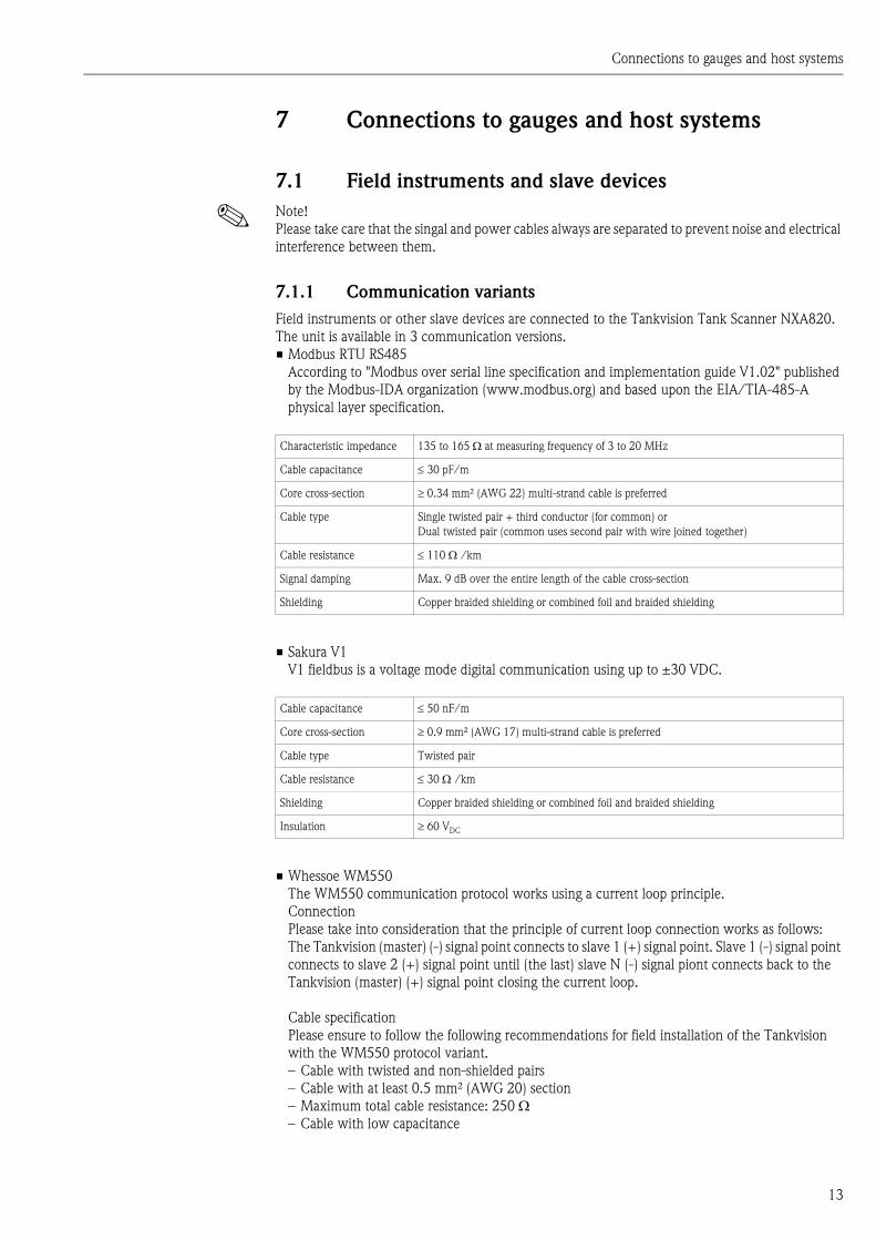
• Modbus RTU RS485

According to "Modbus over serial line specification and implementation guide V1.02" published

by the Modbus-IDA organization (www.modbus.org) and based upon the EIA/TIA-485-A

physical layer specification.

• Sakura V1

V1 fieldbus is a voltage mode digital communication using up to ±30 VDC.

• Whessoe WM550

The WM550 communication protocol works using a current loop principle.

Connection

Please take into consideration that the principle of current loop connection works as follows:

The Tankvision (master) (-) signal point connects to slave 1 (+) signal point. Slave 1 (-) signal point

connects to slave 2 (+) signal point until (the last) slave N (-) signal piont connects back to the

Tankvision (master) (+) signal point closing the current loop.

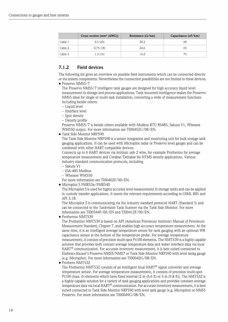
Cable specification

Please ensure to follow the following recommendations for field installation of the Tankvision

with the WM550 protocol variant.

– Cable with twisted and non-shielded pairs

– Cable with at least 0.5 mm² (AWG 20) section

– Maximum total cable resistance: 250 – Cable with low capacitance

Characteristic impedance 135 to 165 at measuring frequency of 3 to 20 MHz

Cable capacitance 30 pF/m

Core cross-section 0.34 mm² (AWG 22) multi-strand cable is preferred

Cable type Single twisted pair + third conductor (for common) or

Dual twisted pair (common uses second pair with wire joined together)

Cable resistance 110 /km

Signal damping Max. 9 dB over the entire length of the cable cross-section

Shielding Copper braided shielding or combined foil and braided shielding

Cable capacitance 50 nF/m

Core cross-section 0.9 mm² (AWG 17) multi-strand cable is preferred

Cable type Twisted pair

Cable resistance 30 /km

Shielding Copper braided shielding or combined foil and braided shielding

Insulation 60 VDC


14

7.1.2 Field devices

The following list gives an overview on possible field instruments which can be connected directly

or via system components. Nevertheless the connection possibilities are not limited to these devices.

• Proservo NMS5/7

The Proservo NMS5/7 intelligent tank gauges are designed for high accuracy liquid level

measurement in storage and process applications. Tank mounted intelligence makes the Proservo

NMS5 ideal for single or multi-task installation, converting a wide of measurement functions

including beside others:

– Liquid level

– Interface level

– Spot density

– Density profile

Proservo NMS5/7 is beside others available with Modbus RTU RS485, Sakura V1, Whessoe

WM550 output. For more information see TI00452G/08/EN.

• Tank Side Monitor NRF590

The Tank Side Monitor NRF590 is a sensor integration and monitoring unit for bulk storage tank

gauging applications. It can be used with Micropilot radar or Proservo level gauges and can be

combined with other HART compatible devices.

Connects up to 6 HART devices via intrinsic safe 2 wire, for example Prothermo for average

temperature measurement and Cerabar/Deltabar for HTMS density applications. Various

industry standard communication protocols, including

– Sakura V1

– EIA-485 Modbus

– Whessoe WM550

For more information see TI00402F/00/EN.

• Micropilot S FMR53x/FMR540

The Micropilot S is used for highly accurate level measurement in storage tanks and can be applied

in custody transfer applications. It meets the relevant requirements according to OIML R85 and

API 3.1B.

The Micropilot S is communicating via the industry standard protocoll HART (Standard 5) and

can be connected to the Tankvision Tank Scanner via the Tank Side Monitor. For more

information see TI00344F/00/EN and TI00412F/00/EN.

• Prothermo NMT539

The Prothermo NMT539 is based on API (American Petroleum Institute) Manual of Petroleum

Measurement Standard, Chapter 7, and enables high accuracy temperature measurement. At the

same time, it is an intelligent average temperature sensor for tank gauging with an optional WB

capacitance sensor at the bottom of the temperature probe. For average temperature

measurement, it consists of precision multi-spot Pt100 elements. The NMT539 is a highly capable

solution that provides both contant average temperature data and water interface data via local

HART® communication. For accurate inventory measurement, it is best suited connected to

Endress+Hauser’s Proservo NMS5/NMS7 or Tank Side Monitor NRF590 with level tankg gauge

(e.g. Micropilot). For more information see TI00042G/08/EN.

• Prothero NMT532

The Prothermo NMT532 consists of an intelligent local HART® signal converter and average

temperature sensor. For average temperature measurement, it consists of precision multi-spot

Pt100 (max. 6) elements which have fixed interval (2 m (6.6 ft) or 3 m (9.8 ft)). The NMT532 is

a highly capable solution for a variety of tank gauging applications and provides constant average

temperature data via local HART® communication. For accurate inventory measurement, it is best

suited connected to Tank Side Monitor NRF590 with level tank gauge (e.g. Micropilot) or NMS5

Proservo. For more information see TI00049G/08/EN.

Cross section (mm² (AWG)) Resistance (/km) Capacitance (nF/km)

Cable 1 0.5 (20) 39.2 60

Cable 2 0.75 (18) 24.6 65

Cable 3 1.3 (16) 14.2 75


15

• Micropilot M FMR2xx

The Micropilot M is used for continuous, non-contact level measurement of liquids, pastes,

slurries and solids. The measurement is not affected by changing media, temperature changes.

– The FMR230 is especially suited for measurement in buffer and process tanks.

– The FMR231 has its strengths wherever high chemical compatibility is required.

– The FMR240 with the small 40 mm (1½") horn antenna is ideally suited for small vessels.

Additionally, it provides an accuracy of ±3 mm (0.12 in).

– The FMR244 combines the advantages of the horn antenna with high chemical resistance.

The 80 mm (3") horn antenna is used additionally in solids.

– The FMR245 - highly resistance up to 200 °C (392 °F) and easy to clean.

The Micropilot M is communicating via the industry standard protocol HART and can be

connected to the Tankvision Tank Scanner via the Tank Side Monitor or an HART to Modbus

converter e.g. by Moore Industries. For more information see TI000345F/00/EN.

• Levelflex M FMP4x

Level Measurement - Continuous level measurement of powdery to granular bulk solids e.g.

plastic granulate and liquids.

– Measurement independent of density or bulk weight, conductivity, dielectric constant,

temperature and dust e.g. during pneumatic filling.

– Measurement is also possible in the event of foam or if the surface is very turbulent.

Interface measurement

Continuous measurement of interfaces between two liquids with very different dielectric

constants, such as in the case of oil and water for example.

The Levelflex M is communicating via the industry standard protocol HART and can be connected

to the Tankvision Tank Scanner via the Tank Side Monitor or an HART to Modbus converter

e.g. by Moore Industries. For more information see TI00358F/00/EN.

• Levelflex FMP5x

– FMP51

Premium device for level and interface measurement in liquids.

– FMP52

Premium device with coated probe for the use in aggressive liquids. Material of wetted parts

FDA listed and USP Class VI compliant.

– FMP54

Premium device for high-temperature and high-pressure applications, mainly in liquids.

Levelflex is communicating via the industry standard protocol HART and can be connected to the

Tankvision Tank Scanner via the Tank Side Monitor or an HART to Modbus converter e.g. by

Moore Industries. For more information see TI01001F/00/EN.

• Cerabar M

The Cerabar M pressure transmitter is used for the following measuring tasks:

– Absolute pressure and gauge pressure in gases, steams or liquids in all areas of process

engineering and process measurement technology.

– High reference accuracy: up to ±0.15%, as PLATINUM version: ±0.075%

Cerabar M is communicating via the industry standard protocol HART and can be connected to

the Tankvision Tank Scanner via the Tank Side Monitor or Proservo.

For more information see TI000436P/00/EN.

• Cerabar S

The Cerabar S pressure transmitter is used for the following measuring tasks:

– Absolute pressure and gauge pressure in gases, steams or liquids in all areas of process

engineering and process measurement technology.


Cerabar S is communicating via the industry standard protocol HART and can be connected to




16

• Deltabar M

The Deltabar M differential pressure transmitter is used for the following measuring tasks:

– Flow measurement (volume or mass flow) in conjunction with primary elements in gases,

vaporss and liquids

– Level, volume or mass measurement in liquids

– Differential pressure monitoring, e.g. of filters and pumps


Deltabar M is communicating via the industry standard protocol HART and can be connected to



• Deltabar S

The Deltabar S differential pressure transmitter is used for the following measuring tasks:

– Flow measurement (volume or mass flow) in conjunction with primary devices in gases, vaporss

and liquids

– Level, volume or mass measurement in liquids

– Differential pressure monitoring, e.g. of filters and pumps


Deltabar S is communicating via the industry standard protocol HART and can be connected to

the Tankvision Tank Scanner via the Tank Side Monitor or an HART to Modbus converter e.g. by

Moore Industries. For more information see TI000382P/00/EN.

• Liquicap M

The Liquicap M FMI5x compact transmitter is used for the continuous level measurement of

liquids.

– Suitable for interface measurement

Liquicap M is communicating via the industry standard protocol HART and can be connected to

the Tankvision Tank Scanner via the Tank Side Monitor or an HART to Modbus converter e.g. by

Moore Industries. For more information see TI00401F/00/EN.

• Whessoe ITGs

• Sakura Endress Float&Tape Transmitter TMD

• Sakura Endress TGM5000

• Sakura Endress TGM4000

• Modbus slave devices

As Modbus is an open protocol there are various system components available which can be

connected to Tankvision Tank Scanner. To do so the so called gauge definition file and the

Modbus map file need to be adapted to the needs. This is a standard procedure and described in

BA00339G/00/EN. Examples for such devices are HART to Modbus converters, PLCs or other

protocol converters e.g. Gauge Emulator by MHT.

! Note!

Remote service access via the Endress+Hauser device configuration tool FieldCare is supported for

the following device combination:

• Tankvision Tank Scanner with Modbus or Sakura V1 communication

• Tank Side Monitor Modbus or Sakura V1 communication and SW version 02.04.00 or later

• HART devices connected to Tank Side Monitor intrinsic safe HART bus and supporting FDT/DTM

or

• Tankvision Tank Scanner with Modbus or Sakura V1 communication

• Proservo NMS5/7 (Modbus or Sakura V1 communication) with

– TCB-6 version 4.27E

– Graphical display operation module

– Modbus communication module COM-5, version 2.0 or

– V1 communication module COM-1 (SRAM-mounted), version 5.01

– HART devices connected to Proservo cannot be reached by FieldCare


17

7.2 Host Systems communication

To transfer and receive data to/from host system the communication variants OPC DA (version

2.05A) and Modbus RS232, Modbus RS485 and Modbus TCP are available.

7.2.1 OPC DA server

See "Tankvision OPC Server", ä 10.

For available parameters see A.1 Parameter list.

7.2.2 Modbus slave via Host Link NXA822

See "Host Link NXA822", ä 9.

For available parameters see A.1 Parameter list.

7.2.3 Connection to Tankvision Professional

To connect to Tankvision Professional a dedicated communication is available. In this case

measured data are transferred as the calculations are performed in Tankvision Professional.

Examples

18

8 Examples

8.1 System architecture

L00-NXA82xxx-02-00-00-en-006

NXA820Tank Scanner

NXA820Tank Scanner

Switch

NXA820Tank Scanner

NXA821Data Concentrator

NXA820 NXA820

NXA822Host Link

NXA820 NXA820 NXA820

Ethernet

DCSOPC Server FieldCareSeveral Printer

for W+M reportsPrinter

Browser

Browser

Browser

DCS

Modbus RTU RS232/485,Modbus TCP

Fieldbus protocol Fieldbus protocol

Operator 1

Operator 2

Operator 3

Fieldbus protocol(e.g. Modbus, V1, WM550)

Examples

19

8.2 Screen examples in Browser

Tank tabular view

Tank details

Examples

20

Trend view

Calculations

21

9 Calculations

Tankvision Tank Scanner can perform various kinds of calculations which are descriped in the

following chapters. The inventory calculations allow the conversion from measured data like level

and temperature to standard data (e.g. Net standard volume or mass). Ther are various standards

for these calculations available differing in the sequence of the calculation or the way compensation

factors are determined (from tables or formula). Today calculations from API (see Text ä 22)

and GB/T (see Text ä 22) are implemented in Tankvision Tank Scanner.

9.1 API Flow Charts

The chart shows the sequence calculations are done according to the API. The different steps are

explained in the following chapters.

L00-NXA82xxx-16-00-00-xx-034

Level

Level

Flow

S&WV

FWL

Base Temp.

Ambient temp.

Air density

air density

Product temp.

Hydrom. corr.

Product Code

S&W

Table & ProductCode

Obs. density &Obs. temp.

Ref. density

FWV

CTSh

Sump/Heelvolume

RemCap AvailVol TOV

GOV

VCF

WAC

Ref. Density

CSW

GSV

NSV

NSW in air

Liquid Mass/NSW in VacuumAir

If Ullage

NoGoZones

convert toInnage

calculateFWV

Floating

API/ASTM

Obs-Refdensity

conversion

S&Wcalculation

Roof

Air corr.calc.

corrections

CalculateRemain cap.

CalculateAvailVol

CalculateTOV

CalculateEquivArea

CalculateEquivArea

TankTop

P-TCT

W-TCT

Tank Shelldetails

RoofDetails

+

-

1.Ullage Conversion

2.Volume calculation

3.Free Water Volume

calculation

4.Tank Shell correction

5.Floating Roofcorrections

7.Volume CorrectionFactor calculation

8.Sediment & Water

calculations

12.Flow calculation

6.Sump/Heel Volume

11.Net Standard Weight

calculation9.

Reference DensityCalculation

10.Net weight in Air

Calculation

Calculations

22

API (American Petroleum Institute)

The American Petroleum Institute, commonly referred to as API, is the largest U.S trade association

for the oil and natural gas industry. It claims to represent about 400 corporations involved in

production, refinement, distribution and many other aspects of the petroleum industry.

The association’s chief functions on behalf of the industry include advocacy and negotiation with

governmental, legal and regulatory agencies; research into economic, toxicological and

environmental effects; establishment and certification of industry standards; and education

outreach. API both funds and conducts research related to many aspects of the petroleum industry.

GB (Chinese national standards)

GB standards are the Chinese national standards issued by the Standardization Administration of

China (SAC), the Chinese National Committee of the ISO and IEC. GB stand for Guobiao, Chinese

for national standard. Mandatory standards are prefixed "GB". Recommended standards are prefixed

"GB/T". A standard number follows "GB" or "GB/T".

Calculations

23

9.1.1 Total Observed Volume - TOV

L00-NXA82xxx-16-00-00-xx-035

The Total Observed Volume (TOV) is determined with the level information and the Tank Capacity

Table (TCT). The TOV is the volume observed at the present (temperature) conditions.

The TCT is a tank specific table created by calibration holding the level to volume transfer

information. To differentiate the TCT for the Product and for the Water the TCT gets marked with

a P (P-TCT).

The level information nedded for this step is in innage which is the normal way the level is

transferred from the gauge. In case the gauge inputs ullage to the system a calculation into innage

is necessary beforehand (Ullage substracted from Mounting position).

Two more information can be derived from TCT and level:

• Remaining Capacity (RemCap) shows how much more product could be pumped into the tank

safely.

• Available Volume (AvailVol) indicates how much product can be pumped out of the tank to the

lowest (defined) possible point e.g. the tank outlet.

9.1.2 Free Water Volume - FWV

L00-NXA82xxx-16-00-00-xx-036

In some cases the tank can also contain water. It can derive from the delivered crude oil, the

processing or by tank breathing. The (innage) water level information together with a Water Tank

Capacity Table (W-TCT) result in the Free Water Volume. It is substracted from the TOV.

Level

RemCap AvailVol TOV

If Ullageconvert to

Innage

CalculateRemain. cap.

CalculateAvailVol

CalculateTOV

TankTop

P-TCT

1.Ullage Conversion

2.TOV calculation

FWLFWV

TOV

calculateFWV

W-TCT

-

3.Free Water Volume

calculation

Calculations

24

9.1.3 Tank Shell Correction - CTSh

• The Tank Shell expands and contracts with temperature changes (compared to TCT calibration

temperature)

• Some countries require CTSh (Correction for Tank Shell temperature effects)

• For heated products the CTSh can be in excess of 0.3% TOV

L00-NXA82xxx-16-00-00-xx-037

! Note!

For more details see ä 45, Chapter "CTSh".

The Tank Shell Correction is a factor which is multiplied with the TOV reduced by the FWV.

9.1.4 Floating Roof Correction - FRC

L00-NXA82xxx-16-00-00-xx-038

A tank can often have a floating roof. A floating roof is called so because it floats on the product

stored in the tank. The roof moves up or down along with product level. Since the roof is floating

on the tank, it displaces some amount of product depending on the weight of the roof and the

density of the product. This displacement in prouct level results in a different apparent level,

introducing an error into the volume calculations. The product volume therefore needs to be

corrected.

A floating roof often has supporting legs. The roof can be rested on these legs when the level is too

low or the tank is empty. This allows maintenance staff to enter below the roof for carrying on tank

maintenance. Based on the product level, the floating roof can be landed on the legs or floating on

the product. However, in a certain range of product level, the floating roof can be pertially landed.

This zone is called "critical zone". In the Tankvision system there can be two critical zones related

to the position of the floating roof legs.

L00-NXA82xxx-16-00-00-xx-039

Base Temp.

Ambient temp.CTSh

Tank Shelldetails

4.Tank Shell correction

air density

Ref. density

NoGoZones

FloatingRoof

corrections

RoofDetails

5.Floating Roofcorrections

B A AA BB

1

3

2

3

1

2

Calculations

25

L00-NXA82xxx-16-00-00-xx-040

Inside critical zone:

3a Apply full FRA

3b Do not Apply FRA

3c Do not calculate FRA

3d Use parcial FRA (interpolate)

! Note!

Floating roofs can already be considered in the TCT.

9.1.5 Sump/Heel/Pipe volume

Volume of the Sump and Pipes are added.

9.1.6 Gross Observed Volume - GOV

L00-NXA82xxx-16-00-00-xx-041

Volu

me

1 3 2

Roof Lan

ded

Hei

ght

Roof T

ake

Off H

eigh

t

LevelRLH

without FRA

withFRA

RTOH

3c

3a

3d

3b

Sump/Pipevolume

TOV

GOV GOV = (TOV - FWV) CTSh FRA + SPV� � � �

FRA

Add Sump/Pipe Volume

Correct for Floating Roof Weight

CTSh Apply CTSh

FWV Subtract Free Water Volume

FloatingRoof

corrections

+

-

Calculations

26

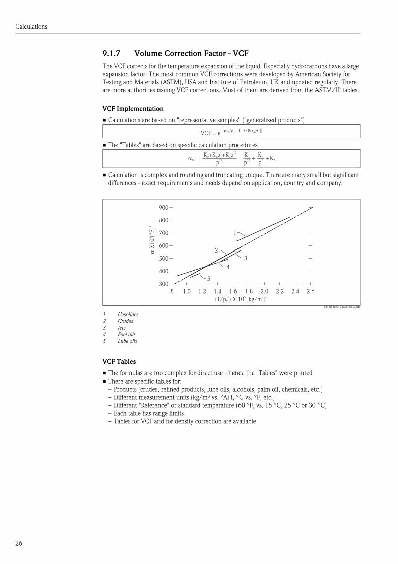
9.1.7 Volume Correction Factor - VCF

The VCF corrects for the temperature expansion of the liquid. Expecially hydrocarbons have a large

expansion factor. The most common VCF corrections were developed by American Society for

Testing and Materials (ASTM), USA and Institute of Petroleum, UK and updated regularly. There

are more authorities issuing VCF corrections. Most of them are derived from the ASTM/IP tables.

VCF Implementation

• Calculations are based on "representative samples" ("generalized products")

• The "Tables" are based on specific calculation procedures

• Calculation is complex and rounding and truncating unique. There are many small but significant

differences - exact requirements and needs depend on application, country and company.

L00-NXA82xxx-16-00-00-xx-044

1 Gasolines

2 Crudes

3 Jets

4 Fuel oils

5 Lube oils

VCF Tables

• The formulas are too complex for direct use - hence the "Tables" were printed

• There are specific tables for:

– Products (crudes, refined products, lube oils, alcohols, palm oil, chemicals, etc.)

– Different measurement units (kg/m³ vs. °API, °C vs. °F, etc.)

– Different "Reference" or standard temperature (60 °F, vs. 15 °C, 25 °C or 30 °C)

– Each table has range limits

– Tables for VCF and for density correction are available

VCF = e[- t(1.0+0.8 t)]� � � �60 60

�60 = = + +K +K p +K p0 1 2

* *2K0 K1 K2

p*2

p*2

p*

900

800

700

600

500

400

300

�TX

10

(°F

)5

-1

.8 1.0 1.2 1.4 1.6 1.8 2.0 2.2 2.4 2.6

(1/p ) X 10 [kg/m ]T

2 5 3 2

1

2

3

4

5

Calculations

27

Most known VCF "Tables"

The Tables are normally grouped in pairs:

• Tables 5 and 6 - ODC resp. VCF °API at 60 °F

• Tables 53 and 54 - ODC resp. VCF kg/m³ at 15 °C

• Tables 24 and 25 - ODC resp. VCF RD 60/60 °F at 60 °F

• Tables 50 and 60 - ODC resp. VCF kg/m³ at 20 °C

Most tables have so called Product Codes:

• A = for generalized crude’s

• B = for refined products

• C = for chemicals

• D = for lube oils

• E = liquefied gases

For chemicals normally a "polynomial equation" is used.

Calculations

28

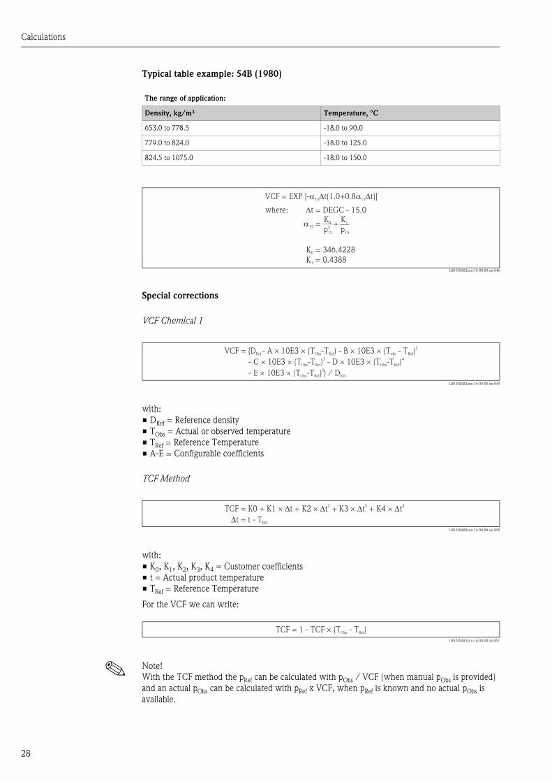
Typical table example: 54B (1980)

L00-NXA82xxx-16-00-00-xx-046

Special corrections

VCF Chemical 1

L00-NXA82xxx-16-00-00-xx-049

with:

• DRef = Reference density

• TObs = Actual or observed temperature

• TRef = Reference Temperature

• A-E = Configurable coefficients

TCF Method

L00-NXA82xxx-16-00-00-xx-050

with:

• K0, K1, K2, K3, K4 = Customer coefficients

• t = Actual product temperature

• TRef = Reference Temperature

For the VCF we can write:

L00-NXA82xxx-16-00-00-xx-051

! Note!

With the TCF method the pRef can be calculated with pObs / VCF (when manual pObs is provided)

and an actual pObs can be calculated with pRef x VCF, when pRef is known and no actual pObs is

available.

The range of application:

Density, kg/m³ Temperature, °C

653.0 to 778.5 -18.0 to 90.0

779.0 to 824.0 -18.0 to 125.0

824.5 to 1075.0 -18.0 to 150.0

VCF = EXP [- t(1.0+0.8 t)]� � � �15 15

K = 346.42280

K = 0.43881

where:

+

�t = DEGC - 15.0

�15 =K0 K1

p15 p15

2

VCF = {D - A 10E3 (T -T ) - B 10E3 (T - T )

- C 10E3 (T -T ) - D 10E3 (T -T )

- E 10E3 (T -T ) } / D

Ref Obs Ref obs Ref

Obs Ref Obs Ref

Obs Ref Ref

� � � �

� � � �

� �

2

3 4

5

TCF = K0 + K1 t + K2� � �� t + K3 t + K4 t2 3 4

�t = t - TRef

TCF = 1 - TCF (T - T )� Obs Ref

Calculations

29

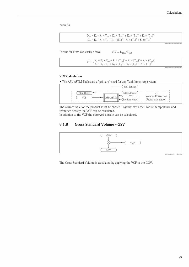
Palm oil

L00-NXA82xxx-16-00-00-xx-052

For the VCF we can easily derive: VCF= DObs/Dref

L00-NXA82xxx-16-00-00-xx-053

VCF Calculation

• The API/ASTM Tables are a "primary" need for any Tank Inventory system

The correct table for the product must be chosen.Together with the Product temperature and

reference density the VCF can be calculated.

In addition to the VCF the observed density can be calculated.

9.1.8 Gross Standard Volume - GSV

L00-NXA82xxx-16-00-00-xx-048

The Gross Standard Volume is calculated by applying the VCF to the GOV.

D = K + K T + K (T ) + K (T ) + K (T )Obs 0 1 Obs 2 Obs 3 Obs 4 Obs� � � �2 3 4

D = K + K T + K (T ) + K (T ) + K (T )ref 0 1 ref 2 ref 3 ref 4 ref� � � �2 3 4

K + K T + K (T ) + K (T ) + K (T )0 1 Obs 2 Obs 3 Obs 4 Obs� � � �2 3 4

K + K T + K (T ) + K (T ) + K (T )0 1 ref 2 ref 3 ref 4 ref� � � �2 3 4VCF =

Product temp.

Table & ProductCode

Ref. density

VCF

Obs. Dens.

API/ASTM

7.Volume CorrectionFactor calculation

GOV

VCF

GSV

Calculations

30

9.1.9 Sediment & Water - S&W

L00-NXA82xxx-16-00-00-xx-072

• Some products have entrained (suspended) sediment and water (S&W)

– i.e. crude’s

• S&W is determined from sample by laboratory method ("Karl-Fisher"-method). The Sediment and

Water percentage (S&W%) determined with the sample is transferred in the Sediment and Water

Fraction (SWF). A correction factor for the product is determined.

As second result the Sediment and Water Volume can be calculated.

Sediment & Water calculation methods

There are 6 methods to calculate S&W

1. SWV = 0

2. SWV = TOV x SWF

3. SWV = (TOV - FWV) x SWF

4. SWV = {(TOV - FWV) x CTSh} x SWF

5. SWV = GOV x SWF

6. SWV = GSV x SWF ("standard" or "default" method)

Where the sediment and water fraction (SWF) is:

L00-NXA82xxx-16-00-00-xx-058

9.1.10 Net Standard Volume - NSV

L00-NXA82xxx-16-00-00-xx-056

Substracting the SWV from the GSV result in Net Standard Volume.

S&WV S&WS&W

calculation

8.Sediment & Water

calculationsCSW

SWF = 1 - (100 - S&W%) / 100= S&W%/100

S&WV S&WCSW

GSV

NSV

S&Wcalculation


calculation

Calculations

31

9.1.11 Density calculations

L00-NXA82xxx-16-00-00-xx-073

We have to distinguish between: observed and reference density

• Observed density is the density of the product at actual (observed) temperature

• Reference density is the density the product would have if we heat/cool it until the reference

temperature (usually 15 °C/60 °F)

• Reference density is used to calculate VCF, FR and mass

• If you know the RefDens you can easily geht the ObDens

ObsDens = RefDens x VCF

• If you know the ObsDens you need (API/ATSM) tables and the sample temperature to get the

RDC (reference density correction factor).

• You can also correct for the thermal expansion of the hydrometer glass (HYC)

RefDens = RDC x ObsDens x HYC

Hydrometer Correction - HYC

L00-NXA82xxx-16-00-00-xx-054

with:

• HYC = Hydrometer correction

• AHYC, BHYC = Thermal expansion coeff. for glass

• t = Temperature of sample

• TCal = Calibration temperature of glass hydrometer

Hydrom. corr.

Product Code

Obs. density &Obs. temp.

Ref. DensityObs-Refdensity

conversion

9.Reference Density

Calculation

HYC = 1.0 - A (t - T ) - B (t - T )HYC Cal HYC Cal� �2

TCal AHYC BHYC

15 °C 0.000 0230 0 0.000 000 020

60 °F 0.000 0127 8 0.000 000 062

Calculations

32

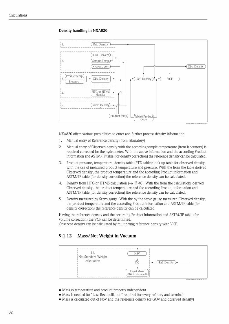
Density handling in NXA820

L00-NXA82xxx-16-00-00-xx-110

NXA820 offers various possibilities to enter and further process density information:

1. Manual entry of Reference density (from laboratory)

2. Manual entry of Observed density with the according sample temperature (from laboratory) is

required corrected for the hydrometer. With the above information and the according Product

information and ASTM/IP table (for density correction) the reference density can be calculated.

3. Product pressure, temperature, density table (PTD table): look up table for observed density

with the use of measured product temperature and pressure. With the from the table derived

Observed density, the product temperature and the according Product information and

ASTM/IP table (for density correction) the reference density can be calculated.

4. Density from HTG or HTMS calculation ( ä 40). With the from the calculations derived

Observed density, the product temperature and the according Product information and

ASTM/IP table (for density correction) the reference density can be calculated.

5. Density measured by Servo gauge. With the by the servo gauge measured Observed density,

the product temperature and the according Product information and ASTM/IP table (for

density correction) the reference density can be calculated.

Having the reference density and the according Product information and ASTM/IP table (for

volume correction) the VCF can be determined.

Observed density can be calculated by multiplying reference density with VCF.

9.1.12 Mass/Net Weight in Vacuum

L00-NXA82xxx-16-00-00-xx-074

• Mass in temperature and product property independent

• Mass is needed for "Loss Reconciliation" required for every refinery and terminal

• Mass is calculated out of NSV and the reference density (or GOV and observed density)

Ref. Density1.

2.

3.

4.

5. Servo Density

Product temp.

Ref. Density VCF

Obs. Density

Obs. Density

Product temp.

Sample Temp.

Pressure

Hydrom. corr.

Obs. Density

HTG or HTMSdensity

Table &ProductCode

Ref. Density

NSV



calculation

Calculations

33

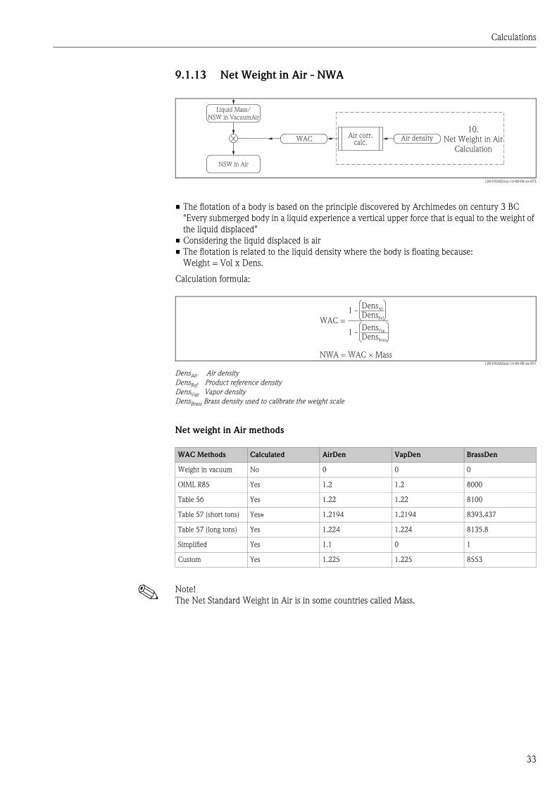
9.1.13 Net Weight in Air - NWA

L00-NXA82xxx-16-00-00-xx-075

• The flotation of a body is based on the principle discovered by Archimedes on century 3 BC

"Every submerged body in a liquid experience a vertical upper force that is equal to the weight of

the liquid displaced"

• Considering the liquid displaced is air

• The flotation is related to the liquid density where the body is floating because:

Weight = Vol x Dens.

Calculation formula:

L00-NXA82xxx-16-00-00-xx-057

DensAir Air density

DensRef Product reference density

DensVap Vapor density

DensBrass Brass density used to calibrate the weight scale

Net weight in Air methods

! Note!

The Net Standard Weight in Air is in some countries called Mass.

Air densityWAC

NSW in Air


Air corr.calc.

10.Net Weight in Air

Calculation

WAC =

NWA = WAC Mass�

1 -

1 -

DensAir

DensRef

DensVap

DensBrass

WAC Methods Calculated AirDen VapDen BrassDen

Weight in vacuum No 0 0 0

OIML R85 Yes 1.2 1.2 8000

Table 56 Yes 1.22 1.22 8100

Table 57 (short tons) Yes 1.2194 1.2194 8393.437

Table 57 (long tons) Yes 1.224 1.224 8135.8

Simplified Yes 1.1 0 1

Custom Yes 1.225 1.225 8553

Calculations

34

9.2 GBT calculation flow chart

The GBT standard is the standard for China.

Main difference is the hydrostatic deformation of the tank not being part of the product TCT but in

a separate table. The VCF and density calculations are based on the same ASTM/IP tables like the

API calculations.

L00-NXA82xxx-16-00-00-xx-033

Product Temp

Ref. Density

FWL

Amb. Temp

Product Temp

Insulation Type

Steel Expa. coef

FRA Mass(G)

S&W

NWA

WCF(Ref. Density - 1.1


NSW/ProductMass/Total

Mass

Obs. Density

Product Temp

Ref. Density

VSPAvailVol**RemCap** LEVEL

Water Densityat 4°C

TOV

VCF

GOV

NSV

Level

HyDC Vol.

FWV**

CTSh**

CSW**

Ref. Density

Sump/PipeVolume

+

+

-

-

Calculate Tankshell correction**

S&WCalculation**

« »Table 59 A.b.DRef. Density Calc.**

Calculate GaugeVolume**

« »Table 60 A.B.DCalculate VCF**

Calculate FWV**

Water TCT

Product TCT

VSP Table

FRA Volume

Calculations

35

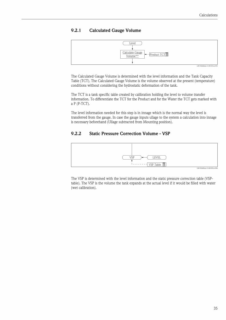
9.2.1 Calculated Gauge Volume

L00-NXA82xxx-16-00-00-xx-093

The Calculated Gauge Volume is determined with the level information and the Tank Capacity

Table (TCT). The Calculated Gauge Volume is the volume observed at the present (temperature)

conditions without considering the hydrostatic deformation of the tank.

The TCT is a tank specific table created by calibration holding the level to volume transfer

information. To differentiate the TCT for the Product and for the Water the TCT gets marked with

a P (P-TCT).

The level information needed for this step is in innage which is the normal way the level is

transferred from the gauge. In case the gauge inputs ullage to the system a calculation into innage

is necessary beforehand (Ullage subtracted from Mounting position).

9.2.2 Static Pressure Correction Volume - VSP

L00-NXA82xxx-16-00-00-xx-094

The VSP is determined with the level information and the static pressure correction table (VSP-

table). The VSP is the volume the tank expands at the actual level if it would be filled with water

(wet calibration).

Level


Product TCT

VSP LEVEL

VSP Table

Calculations

36

9.2.3 Hydrostatic Deformation Correction Volume - HyDC Vol

L00-NXA82xxx-16-00-00-xx-095

The Hydrostatic Deformation Correction Volume is the real from the product fill level created

hydrostatic volume.

It is calculated by correcting the VSP with the ratio of the density of the product versus the water

density.

20 Reference Density at 20 °C (68 °F)

w4 Water Density at 4 °C (39 °F)

The reference density of the Product can be calculated (if not known) with the Observed Density,

the Product/Sample Temperature and the Reference Density Table for the Product.

9.2.4 Total Observed Volume - TOV

L00-NXA82xxx-16-00-00-xx-097

The Total Observed Volume is calculated from the Calculated Gauge Volume and the Hydrostatic

Deformation Correction Volume.

Two more information can be derived from TCT and level:

• Remaining Capacity (RemCap) shows how much more product could be pumped into the tank

safely

• Available Volume (AvailVol) indicates how much product could be pumped out of the tank to the

lowest (defined) possible point e.g. the tank outlet.

9.2.5 Free Water Volume - FWV

L00-NXA82xxx-16-00-00-xx-098

In some cases the tank can also contain water. It can derive from the delivered crude oil, the

processing or by tank breating.

The (innage) water level information together with a Water Tank Capacity Table (W-TCT) result in

the Free Water Volume. It is subtracted from the TOV.

Product Temp

Obs. DensityRef. Density

VSP

Water Densityat 4°C

HyDC Vol.« »Table 59 A.b.D

Ref. Density Calc.**

HyDC = [Vsp ]� r

r w4= [ / ]20

AvailVol**RemCap**

TOV

VSP Vol.+


FWLFWV** Calculate FWV**

Water TCT

Calculations

37

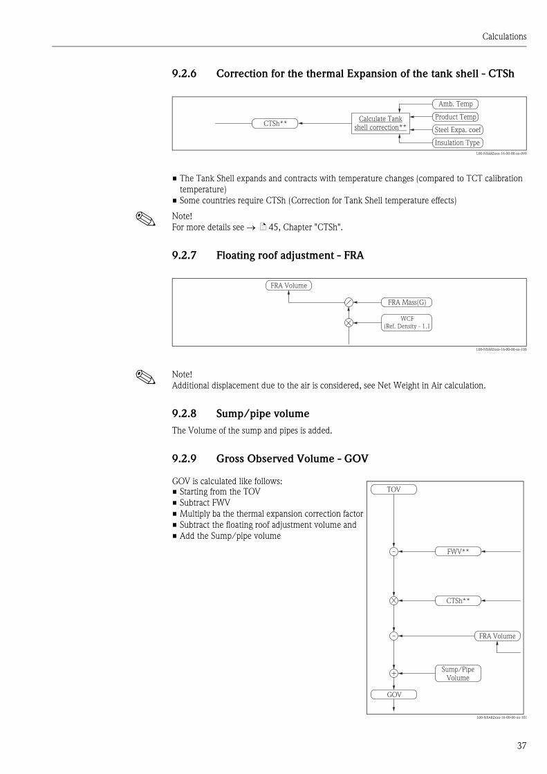
9.2.6 Correction for the thermal Expansion of the tank shell - CTSh

L00-NXA82xxx-16-00-00-xx-099

• The Tank Shell expands and contracts with temperature changes (compared to TCT calibration

temperature)

• Some countries require CTSh (Correction for Tank Shell temperature effects)

! Note!

For more details see ä 45, Chapter "CTSh".

9.2.7 Floating roof adjustment - FRA

L00-NXA82xxx-16-00-00-xx-100

! Note!

Additional displacement due to the air is considered, see Net Weight in Air calculation.

9.2.8 Sump/pipe volume

The Volume of the sump and pipes is added.

9.2.9 Gross Observed Volume - GOV

Amb. Temp

Product Temp

Insulation Type

Steel Expa. coefCTSh**

Calculate Tankshell correction**

FRA Mass(G)


FRA Volume

GOV is calculated like follows:• Starting from the TOV

• Subtract FWV

• Multiply ba the thermal expansion correction factor

• Subtract the floating roof adjustment volume and

• Add the Sump/pipe volume

L00-NXA82xxx-16-00-00-xx-101

FRA Volume

TOV

GOV

FWV**

CTSh**

Sump/PipeVolume

+

-

-

Calculations

38

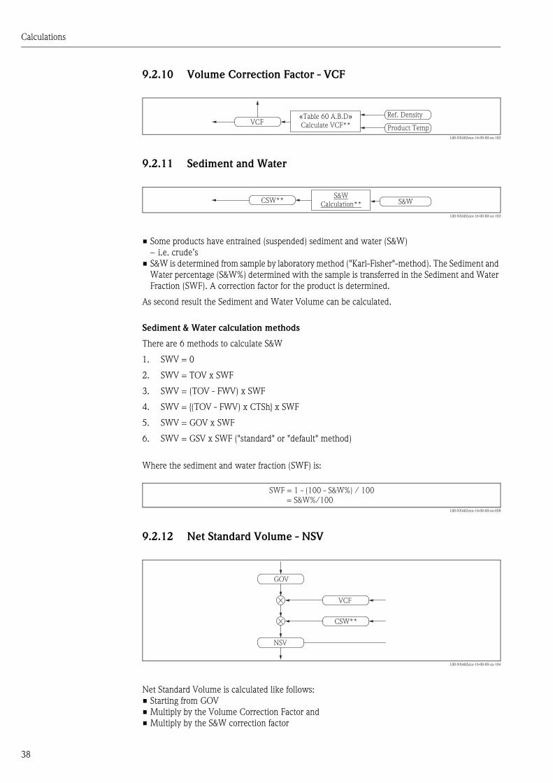
9.2.10 Volume Correction Factor - VCF

L00-NXA82xxx-16-00-00-xx-102

9.2.11 Sediment and Water

L00-NXA82xxx-16-00-00-xx-103

• Some products have entrained (suspended) sediment and water (S&W)

– i.e. crude’s

• S&W is determined from sample by laboratory method ("Karl-Fisher"-method). The Sediment and

Water percentage (S&W%) determined with the sample is transferred in the Sediment and Water

Fraction (SWF). A correction factor for the product is determined.

As second result the Sediment and Water Volume can be calculated.

Sediment & Water calculation methods

There are 6 methods to calculate S&W

1. SWV = 0

2. SWV = TOV x SWF

3. SWV = (TOV - FWV) x SWF

4. SWV = {(TOV - FWV) x CTSh} x SWF

5. SWV = GOV x SWF

6. SWV = GSV x SWF ("standard" or "default" method)

Where the sediment and water fraction (SWF) is:

L00-NXA82xxx-16-00-00-xx-058

9.2.12 Net Standard Volume - NSV

L00-NXA82xxx-16-00-00-xx-104

Net Standard Volume is calculated like follows:

• Starting from GOV

• Multiply by the Volume Correction Factor and

• Multiply by the S&W correction factor

Ref. Density

Product TempVCF

« »Table 60 A.B.DCalculate VCF**

S&WCSW**S&W

Calculation**

SWF = 1 - (100 - S&W%) / 100= S&W%/100

VCF

GOV

NSV

CSW**

Calculations

39

9.2.13 Net Standard Weight - NSW / Product Mass

L00-NXA82xxx-16-00-00-xx-105

Mass is calculated by multiplying NSV with the Reference density.

9.2.14 Net Standard Weight in air - NWA

L00-NXA82xxx-16-00-00-xx-106

The Net Standard Weight in Air is calculated by multiplying the NSV with the Reference Density

reduced by the influence of the Air buoyancy (Reference density - 1.1).

NSW/ProductMass/Total

Mass

NSV

Ref. Density

NWA


NSV

Calculations

40

9.3 Mass Measurement

Today, most hydrocarbons in the western world are bought and sold using volume measurement.

However, in many eastern countries and in some specialised industries, product are sold based on

mass due to traditions in particular markets, so mass calculation can be important in those areas of

trade. Mass-based measurement offers other advantages, since mass is independent of product

temperature and other parameters.

For custody transfer, high accuracy tank gauging is required, and mass-based calculation is often

used.

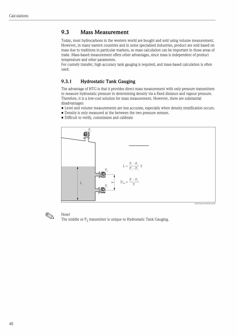
9.3.1 Hydrostatic Tank Gauging

The advantage of HTG is that it provides direct mass measurement with only pressure transmitters

to measure hydrostatic pressure in determining density via a fixed distance and vapour pressure.

Therefore, it is a low-cost solution for mass measurement. However, there are substantial

disadvantages:

• Level and volume measurements are less accurate, especially when density stratification occurs.

• Density is only measured at the between the two pressure sensors.

• Difficult to verify, commission and calibrate

L00-HTGSxxx-05-00-00-xx-001

! Note!

The middle or P2 transmitter is unique to Hydrostatic Tank Gauging.

P3

P2

P1

Y

L = Y

YL

P - P1 3

P - P1 2

P - P1 2

D =obs

Calculations

41

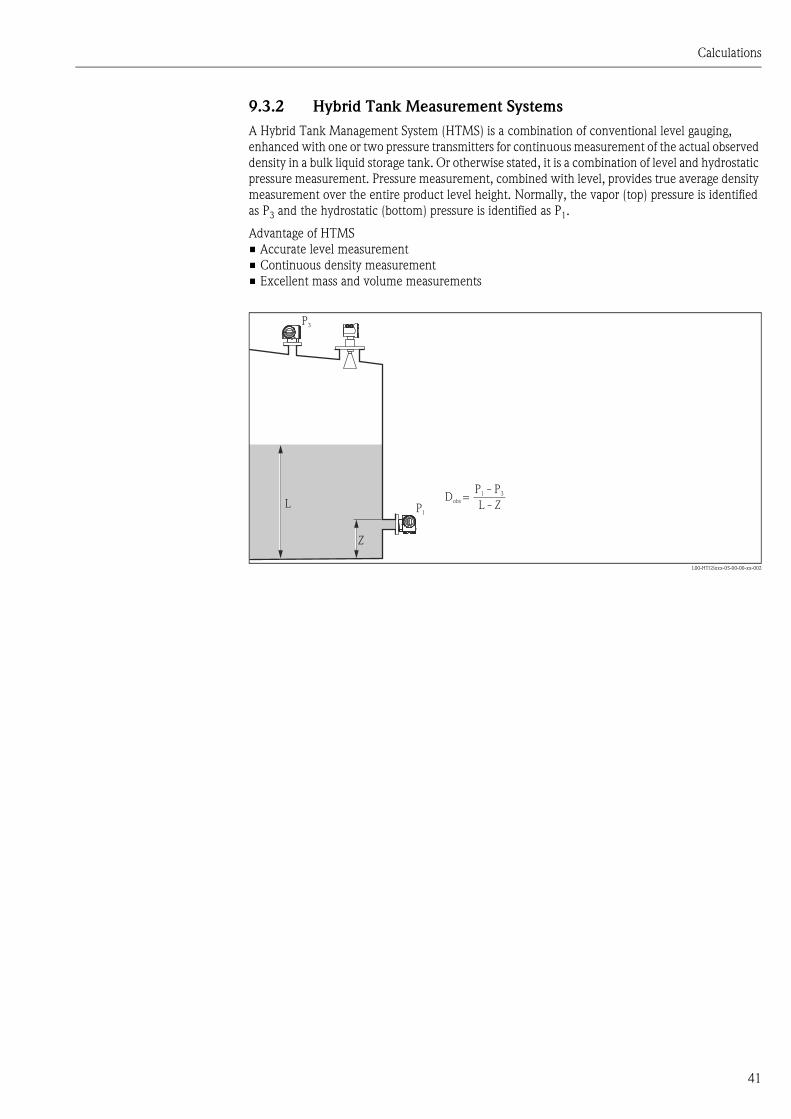
9.3.2 Hybrid Tank Measurement Systems

A Hybrid Tank Management System (HTMS) is a combination of conventional level gauging,

enhanced with one or two pressure transmitters for continuous measurement of the actual observed

density in a bulk liquid storage tank. Or otherwise stated, it is a combination of level and hydrostatic

pressure measurement. Pressure measurement, combined with level, provides true average density

measurement over the entire product level height. Normally, the vapor (top) pressure is identified

as P3 and the hydrostatic (bottom) pressure is identified as P1.

Advantage of HTMS

• Accurate level measurement

• Continuous density measurement

• Excellent mass and volume measurements

L00-HTGSxxx-05-00-00-xx-002

L

Z

P3

P1L - Z

P - P1 3D =obs

Calculations

42

9.4 Calculations for liquefied gases

The mayor difference in the calculation for liquiefied gases compared to liquids is that the gas phase

must be considered. Therefore a calculation for the mass of the product in the gas phase must be

applied.

L00-NXA82xxx-16-00-00-xx-107

9.4.1 Total Mass

9.4.2 MBR method

• The method is based on a specific done by "Moore, Barrett & Redwood" in November 1985. The

calculation procedure was specified for "Whessoe Systems and Controls Ltd.".

• MBR specfy not just the gas calculation, it define a whole process to calculate VCF and RDC.

• This method is only for LPG’s intended but it might also give acceptable results for other Chemical

gasses - as long as the density and temperature are within the specified range.

• Density Input Range: 470 to 610 kg/m³.

• Temperature Inpute Range: -85 to 65 °C (-121 to 149 °F).

• It is not possible to use the M, B & R method for other Reference Temperatures than 15 °C.

Method is based on 10 steps:

1. Measure and input the data

2. VCF Calculation

3. Observed Density calculation

4. Calculate GSV

5. Calculate Liquid Mass

6. Calculate Vapor Volume

7. Calculate Vapor Density

8. Calculate Vapor Mass

9. Calculate Total Mass

10. Calculate Total Weight

Total Mass = Liquid Mass + Vapor Mass

L00-NXA82xxx-16-00-00-xx-108

Vapor densityVapor temp.

Vapor Press.

TankCapacityVaporVol

TOV Ref. Density

Mass in VaporLiquid to

Vapor Ratiocalculation

Densityconversion

Liquid inVapor

Calculation

VaporDetails

Mass in Vapor

WAC

Total MassCalculation

Total massin Vac

Total massin Air

Liquid Mass/NSW in Vacuum

Calculations

43

MBR - Data to be measured (1)

For the LPG application the following data should be real-time measured on the tank(s):

• Product level

• Product Temperature (spot or average)

• Vapor Temperature (spot or average)

• Vapor space pressure - also called "Vapor pressure"

Input data

• The liquid density at 15 °C (59 °F) has to be input by the operator. This density can either be

obtained from a pressurized hydrometer and corrected via an appropriate table or should be

established on basis of chemical analysis.

• The method as implemented in Tankvision also allows the operator to enter Observed or Actual

density as a manual value. Tankvision wil then calculate the corresponding Reference Density.

MBR - VCF Calculation (2)

The following formula shows the calculation method.

L00-NXA82xxx-16-00-00-xx-060

MBR - Observed density (3)

The observed density is calculated using the reference density and the VCF:

• Observed density = Density at 15 °C (59 °F) x VCF

! Note!

The above equation can not be used to calculate the density under reference conditions

(i.e. 15 °C (59 °F)).

MBR - Calculate GSV (4)

The gross standard volume is calculated using the Total observed volume and the VCF

• G.S.V = T.O.V x VCF

MBR - Calculate Liquid Mass (5)

The liquid mass is calculated out of the gross standard volume and the reference density:

• Liquid Mass = G.S.V. x Density at 15 °C (59 °F)

MBR - Calculate Vapor Volume (6)

The vapor volume is obtained using the total tank volume and the liquid total observed volume:

• Vapor volume = Total Tank Volume - TOV

X

Y1

Y2

TR

TT

VO

VO

VD

VD

V2

VCF

V1

TR

TT

=

=

=

=

=

=

=

=

=

=

=

=

=

=

(DENL15 - 500) / 25

0.296-0.2395*X+0.2449167*X*X-0.105*X*X*X+0.01658334*X*X*X*X

368.8+4.924927*X+13.66258*X*X-6.375*X*X*X+1.087503*X*X*X*X

298.2/Y2

(1-TR)^(1/3)

1-1.52816*TT/1.43907*TT*TT-0.81446*TT*TT*TT/0.190454*TT*TT*TT*TT

1-1.52816*TT/1.43907*TT*TT-0.81446*TT*TT*TT/0.190454*TT*TT*TT*TT

(-0.296123+0.386914*TR-0.0427258*TR*TR-0.0480645*TR*TR*TR)/(TR-1.00001)

(-0.296123+0.386914*TR-0.0427258*TR*TR-0.0480645*TR*TR*TR)/(TR-1.00001)

V0*(1-Y1*VD)

V1/V2

VO*(1-Y1*YD)

(TL+273.2)/Y2

(1-TR)^(1/3)

Calculations

44

MBR - Calculate Vapor Density (7)

There are some steps to be followed to get the vapor density

• Molecular weight (MW)

• Critical temperature and pressure

• Reduced temperature and pressure

• Compresibility

• Vapor density

! Note!

The Vapor density is calculated in [kg/m³]

MBR - Calculate Vapor Mass (8)

• The vapor mass (VM) can now be calculated:

MV = Vapor Space x VapDens

• Calculate Total Mass:

Total Mass = Liquid Mass + Vapor Mass

• Equivalent Vapor Liquid Volume

EVLV = Vapor Mass / Liq. Ref. Density

= (D.Ref - 500 / 33.3333)X

= 43 + 4.4 X + 1.35 X - 0.15 X� � �2 3

MW

= 364 + 13.33 X + 8.5 X - 1.833 X� � �2 3

TC

= 43 - 2.283 X + 0.05 X - 0.0667 X� � �2 3

PC

= (TV + 273.2) / TCTR

= (VP + 1.103) / PCPR

=

Locate smallest root of:

Compressibility Z should be in the range of 0.2 to 1 for typical LPG applications.

With:

0.214 - 0.034333 X + 0.005 X - 0.0001667 X� � �2 3

Z - Z + Z (A - b - B ) - A B3 2 2

� �

A = 0.42747 L PR/TR� �2 2

B = 0.08664 PR/TR�L = 1 + (0.48 + 1.574 W - 0.176 W ) (1 - SQRT (TR))� � �

2

W

= (MW (VP + 1.013) / (0.08314 (TV + 273.2) Z� � �VapDen

Calculations

45

9.5 CTSh

9.5.1 What is CTSh

CTSh stands for "Correction for Temperature of the Tank Shell". CTSh is about correcting for when

the temperature of the tank shell is different than the calibration temperature of the tank.

This temperature influence affects the calculated Inventory via (1) the gauge reading, and (2) via a

change in the capacity of the tank as the tank diameter has changed under the temperature effect.

Temperature effect on gauge reading

The temperature effect via the Gauge Reference Height (GRH) affect the level reading and depends on:

• The actual product level in relation to the Gauge Reference Height (GRH),

• The gauge type, for example radar and servo are differently affected,

• The thermal expansion coeficient of the tank steel,

• and the actual tank shell temperature in relation to the tanks shell calibration temperature.

The temperature correction for the Gauge Level reading should be corrected in the Level gauge and

NOT corrected in the Tank Inventorey System.

Reason is that it makes more sense to this correction in the gauge itself:

• Level reading in Gauge ans System should be identical with the same correction applied.

• The required correction depends on the gauge type. A servo, needs for example a different

correction as the temperature effects on the measuring wire in the tank partly compensates the

temperature effects of the tank shell. For a Radar this is not the case.

• Why burden the Tank Iventory system with correction which are gauge specific.

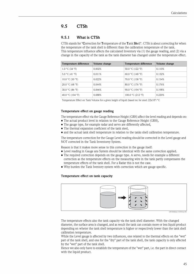
Temperature effect on tank capacity

L00-NXA82xxx-15-00-00-xx-001

The temperature effects also the tank capacity via the tank shell diameter. With the changed

diameter, the surface area is changed, and as result the tank can contain more or less liquid product

depending on wheter the tank shell temperature is higher or respectively lower than the tank shell

calibration temperature.

While the Level gauge is affected by two influences, one related to the thermal effects on the "wet"

part of the tank shell, and one for the "dry" part of the tank shell, the tank capacity is only affected

by the "wet" part of the tank shell.

Hence we also only have to establish the temperature of the "wet" part, i.e. the part in direct contact

with the liquid product.

Temperature difference Volume change Temperature difference Volume change

1.0 °C (34 °F) 0.002% 50.0 °C (122 °F) 0.110%

5.0 °C (41 °F) 0.011% 60.0 °C (140 °F) 0.132%

10.0 °C (50 °F) 0.022% 70.0 °C (158 °F) 0.154%

20.0 °C (68 °F) 0.044% 80.0 °C (176 °F) 0.176%

30.0 °C (86 °F) 0.066% 90.0 °C (194 °F) 0.198%

40.0 °C (104 °F) 0.088% 100.0 °C (212 °F) 0.220%

Temperature Effect on Tank Volume for a given height of liquid (based tec for steel: 22x106/°C

Calculations

46

Wet tank shell temperature

It is unpractical to measure the tank shell temperature for each and individual tank. Hence one

common "estimate" method is used for all tanks. This method is based on the ambien temperature

(Tamb) and the actual liquid product temperature. For most tanks the following expression is

specified in the standards:

L00-NXA82xxx-16-00-00-xx-002

Unfortunately there are also tanks which behave differently. This can be tanks with a real thermal

insulation, but they can also be buried. Hence we had re-write the above equation so we could use

a "insulation factor" If.

L00-NXA82xxx-16-00-00-xx-003

Where:

• Tshell = Temperature of "wet" tank shell

• Tproduct = Temperature of liquid product in tank

• Tambient = Ambient temperature

• If = Insulation Factor

Now we can use the If and use one common equation. Selecting the Insulation factor is simple:

• If = 1.0 for all tanks where the tank is somehow insulated, and

• If = 7/8 for all other tanks

Of course you can modify this setting in the configuration of Tankvision.

! Note!

• In Appendix B you can find a table with some examples as illustration.

• How to obtain the ambient temperature is discussed further on.

Thermal expansion

With the Shell temperature we can now calculated the expansion of the tank capacity. This factor

is indicated with the name CTSh. Late we will see how it applied to the calculated volume.

The CTSh equation depends on the tank type.

Vertical cylindrical tanks

The equation for vertical cylindrical tanks for the volumetric CTSh is relative easy:

L00-NXA82xxx-16-00-00-xx-004

Where:

• = Linear thermal expansion coefficient of tank shell material

• T = Tank Shell Temperature - Tank Calibration temperature

The complexity starts with inconsistencies between the CTSh calculation as specified in various

International standards.

In IP PMP No. 11 (paragraph C.2, page 20) the above equation (1) is simplified to:

L00-NXA82xxx-16-00-00-xx-005

Tshell 7/8 * T + 1/8 * Tproduct ambient=

Tshell I * T + (1 - I ) * Tf product f ambient=

CTSh 1 + 2 * * T + *� �2

T2

=

CTSh 1 + 2 * * T� =

Calculations

47

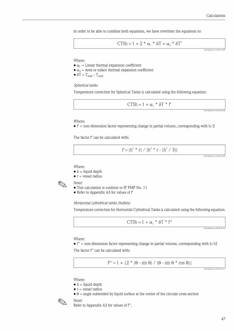
In order to be able to combine both equations, we have rewritten the equations to:

L00-NXA82xxx-16-00-00-xx-007

Where:

• = Linear thermal expansion coefficient

• S = Area or suface thermal expansion coefficient

• T = Tshell - Tcalib

Spherical tanks

Temperature correction for Spherical Tanks is calculated using the following equation:

L00-NXA82xxx-16-00-00-xx-008

Where:

• f’ = non-dimension factor representing change in partial volume, corresponding with h/2

The factor f’ can be calculated with:

L00-NXA82xxx-16-00-00-xx-009

Where:

• h = liquid depth

• r = vessel radius

! Note!

• This calculation is conform to IP PMP No. 11

• Refer to Appendix A3 for values of f’

Horizontal cylindrical tanks (bullets)

Temperature correction for Horizontal Cylindrical Tanks is calculated using the following equation:

L00-NXA82xxx-16-00-00-xx-010

Where:

• f’’ = non-dimension factor representing change in partial volume, corresponding with h/r2

The factor f’’ can be calculated with:

L00-NXA82xxx-16-00-00-xx-011

Where:

• h = liquid depth

• r = vessel radius

• = angle subtended by liquid surface at the centre of the circular cross-section

! Note!

Refer to Appendix A3 for values of f’’.

CTSh 1 + 2 * * T + *� 1 S� T2

=

CTSh 1 + * T * f‘� 1=

f‘ (h * r) / (h * r - (h / 3))2 2 3

=

CTSh 1 + * T * f‘‘� 1=

F‘‘ 1 + 2 * ( - sin ) / ( - sin * cos )� � � � � � �=

Calculations

48

Thermal expansion coefficient(s)

In the previous equations we have used two thermal expansion coefficients:

• = Linear thermal expansion coefficient

• S = Area or surface thermal expansion coefficient

The first one represents the linear thermal expansion of the material of which the tank shell is made.

The second factor represents the squared or area thermal expansion coefficient.

It is of paramount importance that the factor used is in the correct engineering units, i.e. as fraction

per °C or fraction pe °F.

The method for this calculation depends on what equation is to be emulated:

• In case of equation CTSh (3) = 1 + 2 * * T +2 * T2

In this case "S" can be derived from "" by squaring, i.e. "a_tec" = "1_tec"

• In case of equation CTSh (4) = 1 + 2 * * T

In this case "S" should be set to zero.

• For spherical and horizontal cylindrical tanks "S" should be set to zero.

Please also make sure that the exponent value is considered when entering the value in Tankvision.

For example if "" is set to be equal to "1.6 10^-5", while as engineering units shown is "10EE-7/

°C", the "" value to be entered is "160".

Calculations

49

9.5.2 Measurement of ambient temperature

The CTSh should be calculated automatically, which is only possible if we also have the actual

ambient temperature measured automatically.

Tankvision is capable of integration of this temperature from field equipment. It can redistribute this

information over the whole or part of the Tank Farm. This makes it possible to use one ambient

temperature sensor and use the measure temperature for one or more tanks within the same

Tankvision system.

Automatic measurement of ambient temperature on site

Exact recommendations on the location, installation and accuracy of the Ambient Temperature

sensor are vague. The sensor should be located in the outside environment, be protected from direct

sun shine, rain and wind, and preferable be approximately 1 meter (3 ft) from any building or large

object.

An external Ambient Temperature sensor can be connected via:

• NRF590 – for example by adding an extra HART converter with temperature sensor, or by using

the optional RTD input

• Proservo NMS53x – as above

Other methods may also possible be possible, depending on installed equipment and used field

protocol. Please consult Endress+Hauser.

Later we will also see that there is a special setting in Tankvision where we can disable fail

propagation if the ambient temperature doesn’t work. After all it would be pretty horrific if the

calculated inventory data of all tanks is suddenly useless, just because one sensor fails.

Manual entry of ambient temperature

It is also possible to enter the ambient Temperature manual.

This could be used, for either verifying the CTSh calculations, or in the unlikely case the ambient

temperature is in fail.

9.6 Alcohol calculations

9.6.1 The OIML R22

The OIML R22, as issued in 1975 deals with the calculations for the basic data "relating to the

density and to the alcoholic strengths by mass and by volume of mixtures of water and ethanol". As

per OILM R22 standards the range is -20 to +40 °C (-4 to +104 °F) and defines the following:

• Table 1:

Gives the Observe density as a function of the temperature and the alcohol strength by mass

• Table 2:

Gives the Observe density as a function of the temperature and the alcohol strength by volume

• Table 3A and 3B:

Gives the standard (reference) density at 20 °C (68 °F) (Table 3A) and the alcoholic strength by

volume (Table 3B) as a function of the alcoholic strength by mass


Gives the standard density at 20 °C (68 °F) (Table 4A) and the alcoholic strength by mass (Table

4B) as a function of the alcohol strength by volume


Gives the acloholic strength by mass (Table 5A) and the alcoholic strength by volume (Table 5B)

as a function of the observe density at 20 °C (68 °F)

• Table 6:

Gives the alcoholic strength by mass as a function of the observe density and temperature

• Table 7:

Gives the alcoholic strength by volume as a function of the observe density and temperature


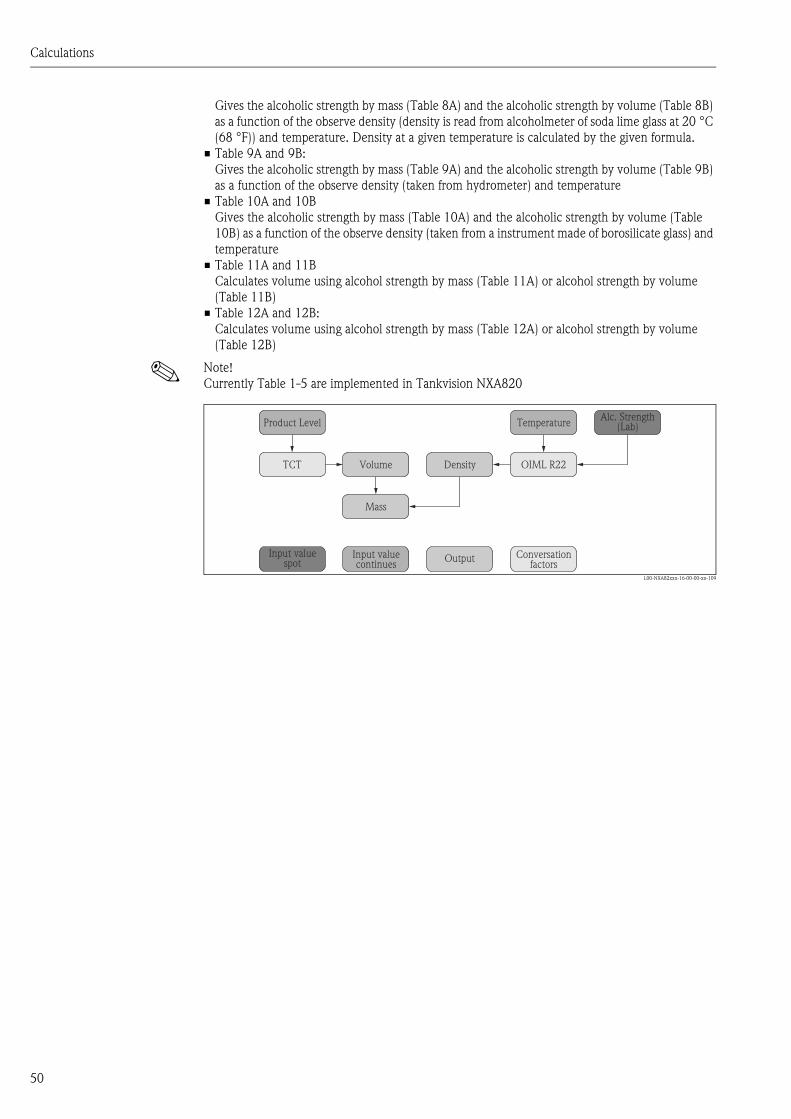
Calculations

50

Gives the alcoholic strength by mass (Table 8A) and the alcoholic strength by volume (Table 8B)

as a function of the observe density (density is read from alcoholmeter of soda lime glass at 20 °C

(68 °F)) and temperature. Density at a given temperature is calculated by the given formula.


Gives the alcoholic strength by mass (Table 9A) and the alcoholic strength by volume (Table 9B)

as a function of the observe density (taken from hydrometer) and temperature

• Table 10A and 10B

Gives the alcoholic strength by mass (Table 10A) and the alcoholic strength by volume (Table

10B) as a function of the observe density (taken from a instrument made of borosilicate glass) and

temperature

• Table 11A and 11B

Calculates volume using alcohol strength by mass (Table 11A) or alcohol strength by volume

(Table 11B)


Calculates volume using alcohol strength by mass (Table 12A) or alcohol strength by volume

(Table 12B)

! Note!

Currently Table 1-5 are implemented in Tankvision NXA820

L00-NXA82xxx-16-00-00-xx-109

Product Level

Input valuecontinues

Input valuespot Output Conversation

factors

TemperatureAlc. Strength

(Lab)

Mass

TCT Volume OIML R22Density

Calculations

51

9.7 Annex A.1

ID PARAMETER OPC ID PARAMETER OPC

622 P_LEVEL Level

(default)

1634 TEMP_1 SPOT_TEMP_1

(dynamic)

623 S_LEVEL SecondaryLevel

(dynamic)


(dynamic)

624 W_LEVEL WaterLevel

(default)


(dynamic)

625 P_TEMP Temperature

(default)


(dynamic)

626 V_TEMP VaporTemperature

(default)


(dynamic)

660 A_TEMP AmbientTemperature

(default)


(dynamic)

627 V_PRESS VaporPressure

(default)


(dynamic)

628 P_OBS_D CALC_OBSERVED_DENSITY

(default)


(dynamic)

661 P_REF_D CALC_REF_DENSITY

(default)


(dynamic)

690 P_PRESS_A - 1643 TEMP_10 SPOT_TEMP_10

(dynamic)

691 P_PRESS_G - 1644 TEMP_11 SPOT_TEMP_11

(dynamic)

692 P_PRESS - 1645 TEMP_12 SPOT_TEMP_12

(dynamic)

693 V_PRESS_A - 1646 TEMP_13 SPOT_TEMP_13

(dynamic)

694 V_PRESS_G - 1647 TEMP_14 SPOT_TEMP_14

(dynamic)

717 TOT_OBS_VOL TOT_OBSERVED_VOLUME

(default)


(dynamic)

718 REM_CAP_TANK REM_CAPACITY_TANK

(default)


(dynamic)

719 AVAIL_VOL AVAIL_VOLUME

(default)

2101 ALCOHOL_BY_MASS AlcoholByMass

(default)

720 SED_W_VOL SED_WATER_VOL

(default)

2102 ALCOHOL_BY_VOLUME AlcoholByVolume

(default)

721 P_LVLCHNG_RATE PROD_LVLCHANGE_RATE

(default)

1551 SAMPLE_TEMPERAURE SampleTemperature

(default)

722 TOTOBS_FLW_RATE TOTOBSERVED_FLOT_RATE

(default)

2601 GP01 GP01

(dynamic)

723 NETSTD_FLW_RATE NETSTD_FLOW_RATE

(default)

2602 GP02 GP02

(dynamic)

724 TOTMASS_FLW_RATE TOTMASS_FLOW_RATE

(default)

2603 GP03 GP03

(dynamic)

725 FREE_W_VOL FREE_WATER_VOL

(default)

2604 GP04 GP04

(dynamic)

726 GROSSS_OBS_VOL GROSS_OBS_VOLUME

(default)

2605 GP05 GP05

(dynamic)

752 TOT_STD_VOL TOTAL_STD_VOLUME

(default)

2606 GP06 GP06

(dynamic)

Calculations

52

dynamic = exported via OPC only when scanned via field scan or set to manual value

754 VCF VCF

(default)

2607 GP07 GP07

(dynamic)

756 MASS_VAPR MASS_VAPOUR

(default)

2608 GP08 GP08

(dynamic)

760 NET_WGHT_AIR NET_WEIGHT_AIR

(default)

2609 GP09 GP09

(dynamic)

761 NET_STD_WGHT NET_STD_WEIGHT

(default)

2610 GP10 GP10

(dynamic)

762 R_ROOF_ADJUS FLOAT_ROOF_ADJUS

(default)

2611 GP11 GP11

(dynamic)

763 F_ROOF_POS FLOAT_ROOF_POS

(default)

2612 GP12 GP12

(dynamic)

774 TNK_SHELL_CORR TANK_SHELL_CORREC

(default)

2613 GP13 GP13

(dynamic)

727 GROSS_STD_VOL GROSS_STD_VOLUME

(default)

2614 GP14 GP14

(dynamic)

728 NET_STD_VOL NET_STD_VOL

(default)

2615 GP15 GP15

(dynamic)

729 P_MASS PRODUCT_MASS 2616 GP16 GP16

(dynamic)

730 TOT_MASS TOTAL_MASS

(default)

2650 PROTOCOL_ALARM_1 -

1592 VAPOR_ROOM_VOL - 2651 PROTOCOL_ALARM_2 -



2654 PERCENTAGE_LEVEL -

ID PARAMETER OPC ID PARAMETER OPC

Calculations

53

9.8 Annex A.2

Insulation factors for various tank geometries

L00-NXA82xxx-16-00-00-xx-014

Fixed RoofTank

d = dry

Ts = Ifw * Tp + (1 - Ifw) * Ta

v = vapor

a = ambient

w = wet

TS =

RecommendedInsulationFactor (IFw)

Ifw = (.825) Ifw = 1.0 Ifw = 1.0 Ifw = 1.0 Ifw = 1.0 Ifw =

p = product

InsulatedTank

Tank withStill. Well

(SW)

Tank withInternalFR & SW

ExternalFloating RoofTank with SW

Floating orNo Roof -

Directmeasurement

TV TV TVTd

Ta Ta Ta Ta

Ta Ta

TP TP TP TP TPTw

Td

Tw TP

TV

* Tp + * Ta78

18

78

78

* Tp + * Ta78

18Tp Tp Tp Tp

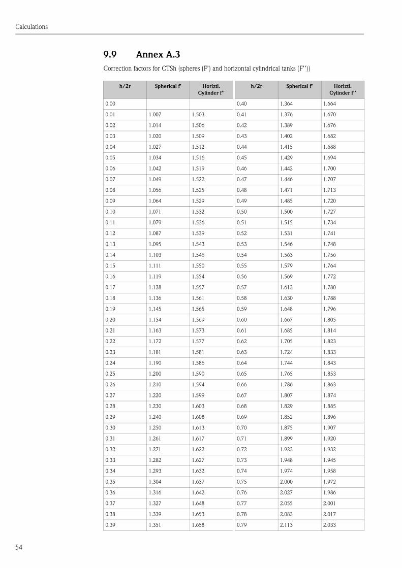
Calculations

54

9.9 Annex A.3

Correction factors for CTSh (spheres (F’) and horizontal cylindrical tanks (F’’))

h/2r Spherical f’ Horiztl.

Cylinder f’’

h/2r Spherical f’ Horiztl.

Cylinder f’’

0.00 0.40 1.364 1.664

0.01 1.007 1.503 0.41 1.376 1.670

0.02 1.014 1.506 0.42 1.389 1.676

0.03 1.020 1.509 0.43 1.402 1.682

0.04 1.027 1.512 0.44 1.415 1.688

0.05 1.034 1.516 0.45 1.429 1.694

0.06 1.042 1.519 0.46 1.442 1.700

0.07 1.049 1.522 0.47 1.446 1.707

0.08 1.056 1.525 0.48 1.471 1.713

0.09 1.064 1.529 0.49 1.485 1.720

0.10 1.071 1.532 0.50 1.500 1.727

0.11 1.079 1.536 0.51 1.515 1.734

0.12 1.087 1.539 0.52 1.531 1.741

0.13 1.095 1.543 0.53 1.546 1.748

0.14 1.103 1.546 0.54 1.563 1.756

0.15 1.111 1.550 0.55 1.579 1.764

0.16 1.119 1.554 0.56 1.569 1.772

0.17 1.128 1.557 0.57 1.613 1.780

0.18 1.136 1.561 0.58 1.630 1.788

0.19 1.145 1.565 0.59 1.648 1.796

0.20 1.154 1.569 0.60 1.667 1.805

0.21 1.163 1.573 0.61 1.685 1.814

0.22 1.172 1.577 0.62 1.705 1.823

0.23 1.181 1.581 0.63 1.724 1.833

0.24 1.190 1.586 0.64 1.744 1.843

0.25 1.200 1.590 0.65 1.765 1.853

0.26 1.210 1.594 0.66 1.786 1.863

0.27 1.220 1.599 0.67 1.807 1.874

0.28 1.230 1.603 0.68 1.829 1.885

0.29 1.240 1.608 0.69 1.852 1.896

0.30 1.250 1.613 0.70 1.875 1.907

0.31 1.261 1.617 0.71 1.899 1.920

0.32 1.271 1.622 0.72 1.923 1.932

0.33 1.282 1.627 0.73 1.948 1.945

0.34 1.293 1.632 0.74 1.974 1.958

0.35 1.304 1.637 0.75 2.000 1.972

0.36 1.316 1.642 0.76 2.027 1.986

0.37 1.327 1.648 0.77 2.055 2.001

0.38 1.339 1.653 0.78 2.083 2.017

0.39 1.351 1.658 0.79 2.113 2.033

Calculations

55

9.10 Annex A.4

Example CTSh calculations

9.11 Documentation

Tank Type Vertical Cylindrical Vertical Cylindrical Vertical Cylindrical Spherical Vertical Cylindrical

Vessel Radius n.a. n.a. n.a. 17.253 n.a.

Product Level n.a. n.a. n.a. 4.6 n.a.

1 (apha) 6.2 x 10^-6 6.2 x 10^-6 0.000011 110 x 10^-7 6.2 x 10^-6

s 4.01E-09 0 0 n.a. 4.01E-09

Tcal 60 °F 60 °F 15 °C 20 °C 60 °F

Tprod 300 °F 300 °F -43 °C 23.5 °C 88.3 °F

Tamb 70 °F 70 °F n.a. 74.5 °F

Ifs 0.875 0.875 1 1 0.875

CTSh 1.00279801 1.0026195 0.998724 1.000047 1.00032

Document Instrument Description

TI00419G/00/EN Tankvision Inventory Management System wich completely integrated

software for operation via standard web browser

TI00452G/08/EN Proservo NMS5 Intelligent tank gauge with high accuracy performance

Liquid level, I/F, Density & Density Profile

TI00402F/00/EN Tank Side Monitor NRF590 Field device for tank sensor operation and monitoring and for

integration into inventory control system

TI00344F/00/EN Micropilot S FMR53x Continuous level transmitter for continuous and non-contact

precision level measurement. For custody transfer and

inventory control applications with NMi- and PTB-approvals

TI00412F/00/EN Micropilot S FMR540 Continuous level transmitter for continuous and non-contact

precision level measurement. For custody transfer and

inventory control applications with NMi and PTB approvals

TI00042G/08/EN Prothermo NMT539 Intrinsically safe multi-signal converter with precision ave-

rage temperature and water bottom sensor for inventory

control and custody transfer applications

TI00049G/08/EN Prothermo NMT532 Intrinsically safe multi-signal converter with precision ave-

rage temperature sensor for inventory control

TI00345F/00/EN Micropilot M FMR23x, FMR24x Continuous and non-contact level measurement. Cost-effec-

tive 4 to 20 mA 2-wire technology. Suitable for hazardous

locations.

TI00358F/00/EN Levelflex M FMP40 Continuous Level Transmitter for:

- Level Measurement in Bulk Solids and Liquids

- Interface Measurement in Liquids

TI01001F/00/EN Levelflex FMP51, FMP52, FMP54 Level and interface measurement in liquids

TI00436P/00/EN Cerabar M PMC51, PMP51, PMP55 Pressure transmitter with ceramic and metal sensors;

With analog electronics or communication via HART, PRO-

FIBUS PA or FOUNDATION Fieldbus

TI00383P/00/EN Cerabar S PMC71, PMP71, PMP75 Pressure transmitter with ceramic and metal sensors

Overload-resistant and function-monitored; Communica-

tion via HART, PROFIBUS PA or FOUNDATION Fieldbus

TI00434P/00/EN Deltabar M PMD55 Differential presure transmitter with metal sensor

Communication via HART, PROFIBUS PA or FOUNDA-

TION Fieldbus

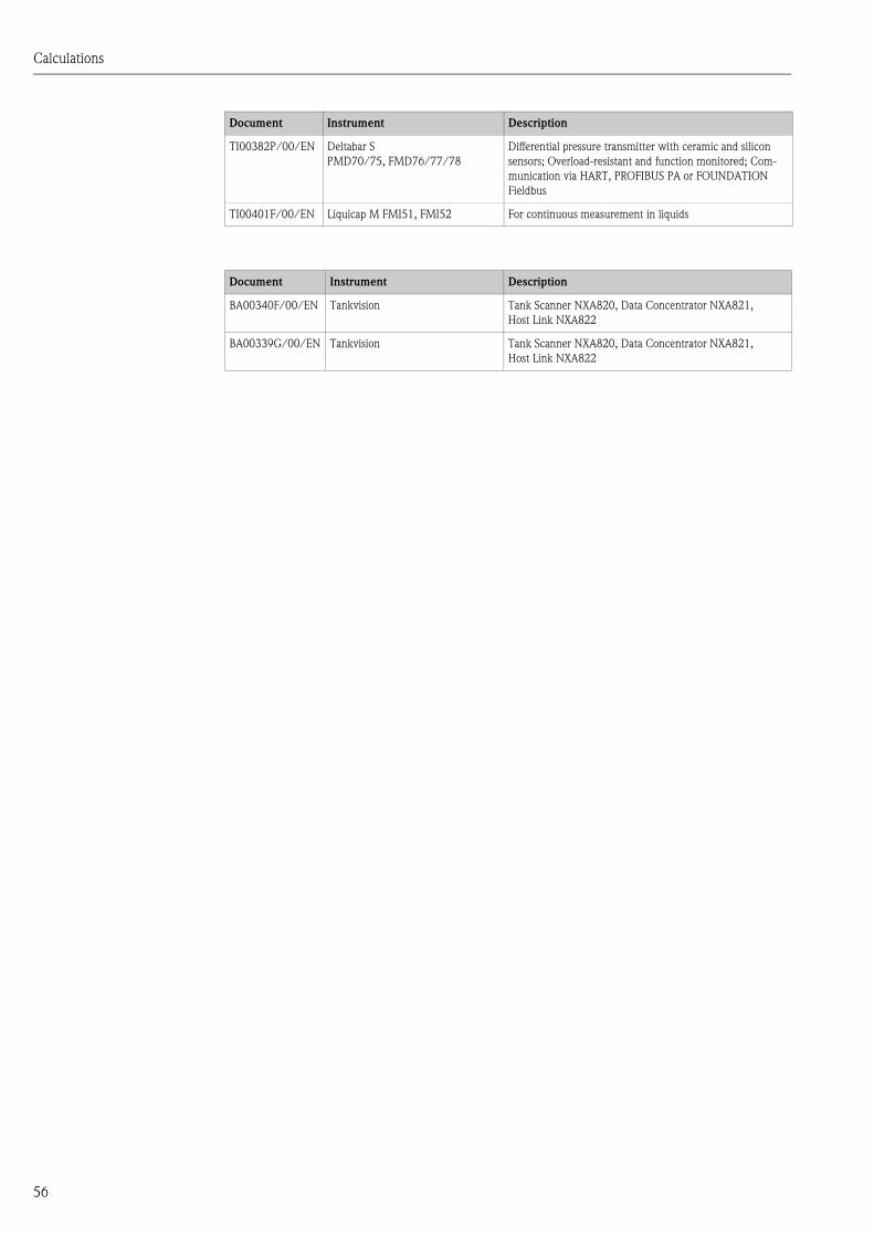
Calculations

56

TI00382P/00/EN Deltabar S

PMD70/75, FMD76/77/78

Differential pressure transmitter with ceramic and silicon

sensors; Overload-resistant and function monitored; Com-

munication via HART, PROFIBUS PA or FOUNDATION

Fieldbus

TI00401F/00/EN Liquicap M FMI51, FMI52 For continuous measurement in liquids


BA00340F/00/EN Tankvision Tank Scanner NXA820, Data Concentrator NXA821,

Host Link NXA822

BA00339G/00/EN Tankvision Tank Scanner NXA820, Data Concentrator NXA821,

Host Link NXA822


Calculations

57

Calculations

58

Calculations

59

www.endress.com/worldwide

BA00426G/00/EN/01.12

71193832

CCS/FM+SGML 9.0/ProMoDo 71193832

Date post:	28-May-2018
Category:	Documents
Upload:	doankhanh
View:	329 times
Download:	3 times

Tankvision Tank Scanner NXA820, Data Concentrator NXA821 ... · Tank Scanner NXA820, Data...

Documents