1 Targeting alternative measures of inflation under uncertainty about inflation expectations and exchange rate pass-through Vincenzo Cassino, Aaron Drew and Sharon McCaw * 1. Introduction It has become increasingly common among central banks to specify the operational goal of monetary policy as the maintenance of price stability. For example, the European Central Bank (ECB) recently announced that its goal for monetary policy is to keep inflation below two percent per annum over the medium term. In translating the operational goal into practice, it must be decided which price index is to be targeted. Theory suggests that if the primary cost of inflation arises from consumers’ uncertainty regarding the future purchasing power of their incomes, then monetary policy should strive to stabilise a utility-constant consumer price index. In the absence of such ideal indices, central banks have opted to target some available index of consumer prices. As consumer price indices are independently calculated by statistical agencies, they are seen as credible targets for policy. This is perhaps their primary advantage. However, the disadvantage of targeting consumer prices is that the aggregate index is often affected by price movements in sub- components that do not reflect the ‘underlying’ trend in inflation. Setting policy at all times based upon movements in aggregate consumer prices could then lead to sub-optimal outcomes. In recognition of this problem, central banks do not in practice strive to meet their CPI inflation targets at all times (see Debelle (1997)). Instead, operational flexibility is afforded to the central bank, arising in two main guises. The first is to target CPI inflation subject to ‘caveats’ for price movements in the index that are seen as extraordinary (for example, as in New Zealand and Canada). The second is to allow the central bank to meet the inflation target over a somewhat flexible period of time (for example, in the ‘medium’ term at the ECB, and ‘over the cycle’ at the Reserve Bank of Australia). A central bank afforded operational flexibility in policy making, explicitly or implicitly, needs to take into account what is often termed underlying or ‘core’ inflation. Many alternative methodologies have been proposed to measure core inflation. The key concept behind these measures is that the central bank should counter only persistent sources of inflationary pressures, as these become ingrained into inflation expectations. Consequently, the inflation control problem is difficult to manage if core inflation ‘gets away’ from the inflation target. In contrast, by definition temporary inflation shocks will not have ongoing effects, and therefore the consequences for the monetary authority of ignoring them are less severe. In the macro model that lies at the heart of the Reserve Bank of New Zealand’s Forecasting and Policy System, FPS, core inflation is defined as the rate of inflation in the price of domestically produced and consumed goods. This rate of inflation is driven principally by the deviation of aggregate demand for goods and services from the economy’s supply capacity. However, for small open economies, movements in the nominal exchange rate, via their direct effect on the price of imported goods, cause a significant part of the variation in consumer price indices. The model’s definition of CPI inflation incorporates these direct exchange rate effects, while the core inflation measure does not. * Economics Department, Reserve Bank of New Zealand, P O Box 2498, Wellington, New Zealand. Correspondence should be addressed to Aaron Drew. Email: [email protected]. The views expressed in this paper are those of the authors and do not necessarily represent the views of the Reserve Bank of New Zealand. This work should be treated as work in progress and should not be quoted without permission of the authors.
Transcript
1
Targeting alternative measures of inflation under uncertainty aboutinflation expectations and exchange rate pass-through
Vincenzo Cassino, Aaron Drew and Sharon McCaw *
1. Introduction
It has become increasingly common among central banks to specify the operational goal of monetarypolicy as the maintenance of price stability. For example, the European Central Bank (ECB) recentlyannounced that its goal for monetary policy is to keep inflation below two percent per annum over themedium term. In translating the operational goal into practice, it must be decided which price index isto be targeted. Theory suggests that if the primary cost of inflation arises from consumers’uncertainty regarding the future purchasing power of their incomes, then monetary policy shouldstrive to stabilise a utility-constant consumer price index. In the absence of such ideal indices, centralbanks have opted to target some available index of consumer prices.
As consumer price indices are independently calculated by statistical agencies, they are seen ascredible targets for policy. This is perhaps their primary advantage. However, the disadvantage oftargeting consumer prices is that the aggregate index is often affected by price movements in sub-components that do not reflect the ‘underlying’ trend in inflation. Setting policy at all times basedupon movements in aggregate consumer prices could then lead to sub-optimal outcomes. Inrecognition of this problem, central banks do not in practice strive to meet their CPI inflation targetsat all times (see Debelle (1997)). Instead, operational flexibility is afforded to the central bank,arising in two main guises. The first is to target CPI inflation subject to ‘caveats’ for pricemovements in the index that are seen as extraordinary (for example, as in New Zealand and Canada).The second is to allow the central bank to meet the inflation target over a somewhat flexible period oftime (for example, in the ‘medium’ term at the ECB, and ‘over the cycle’ at the Reserve Bank ofAustralia).
A central bank afforded operational flexibility in policy making, explicitly or implicitly, needs to takeinto account what is often termed underlying or ‘core’ inflation. Many alternative methodologieshave been proposed to measure core inflation. The key concept behind these measures is that thecentral bank should counter only persistent sources of inflationary pressures, as these becomeingrained into inflation expectations. Consequently, the inflation control problem is difficult tomanage if core inflation ‘gets away’ from the inflation target. In contrast, by definition temporaryinflation shocks will not have ongoing effects, and therefore the consequences for the monetaryauthority of ignoring them are less severe.
In the macro model that lies at the heart of the Reserve Bank of New Zealand’s Forecasting andPolicy System, FPS, core inflation is defined as the rate of inflation in the price of domesticallyproduced and consumed goods. This rate of inflation is driven principally by the deviation ofaggregate demand for goods and services from the economy’s supply capacity. However, for smallopen economies, movements in the nominal exchange rate, via their direct effect on the price ofimported goods, cause a significant part of the variation in consumer price indices. The model’sdefinition of CPI inflation incorporates these direct exchange rate effects, while the core inflationmeasure does not.
*Economics Department, Reserve Bank of New Zealand, P O Box 2498, Wellington, New Zealand.Correspondence should be addressed to Aaron Drew. Email: [email protected]. The views expressed in thispaper are those of the authors and do not necessarily represent the views of the Reserve Bank of New Zealand.This work should be treated as work in progress and should not be quoted without permission of the authors.
2
If exchange rate movements affect only the level of the CPI, and not inflation expectations, thenexchange rate pass-through constitutes the type of shock that core inflation measures aim to remove.In this case, a priori, we would expect that ‘looking through’ these short-lived effects would lead tosuperior macroeconomic outcomes. This is examined in Svensson (1998), where a model of a smallopen economy is used to compare ‘flexible’ policy rules that target CPI inflation, against those thattarget domestic price inflation. Svensson’s results largely confirm our intuition - the variance in CPIinflation and the real exchange rate is lower when targeting CPI inflation, whilst the variance in realoutput and nominal interest rates are lower when targeting domestic price inflation.
We might expect that agents face a signal extraction problem in the real world as to how much ofobserved inflation constitutes ‘core’ inflation. Given this problem, we do not know exactly howagents form their expectations of inflation. Hence, there is no guarantee that agents’ perceptions ofcore inflation are the same as that of the monetary authority. In Conway et al. (1998), stochasticsimulations of FPS are used to explore the implications of this uncertainty in the context of CPIversus core domestic price inflation targeting. The result found in Svensson (op. cit.) was largelyupheld. That is, whether direct exchange rate price effects influence inflation expectations or only thelevel of CPI inflation, and regardless of whether the monetary authority perceives this correctly,targeting domestic inflation reduces the variability in all macro variables except for CPI inflation.
This paper extends the work presented in Conway et al. in several dimensions. Firstly, followingrecent development of the FPS core model, the stochastic disturbances applied are a more completerepresentation of the shocks the New Zealand economy has faced historically. Secondly, we examinethe performance of the model economy under a broader range of policy rules. Finally we add anotherimportant dimension of uncertainty to the problem – that of the speed of exchange rate pass-through.Reflecting conventional ‘stylised facts’, the exchange rate transmission channel of monetary policy inFPS affects CPI inflation more quickly than the aggregate demand transmission channel.Nevertheless, the exchange rate transmission channel is still slow relative to other stylised modelssuch as that in Svensson (1998). This reflects only New Zealand’s recent experience. Thetransmission of exchange rate or foreign price movements into domestic import prices has been quitevariable over time. Given this uncertainty about the speed of exchange rate pass-through, coupledwith uncertainty about how agents form their inflation expectations, we examine whether it is still thecase that preferable macroeconomic outcomes are attainable under domestic price inflation targeting.
Our results suggest that under the standard forward-looking inflation targeting policy rule used in FPS– a rule that is used to prepare the Bank’s economic projections – it is indeed still the case thattargeting core inflation results in superior macroeconomic outcomes. We also examine theperformance of the model economy under three alternative, descriptively accurate policy rules.1 Inparticular, we consider an inflation-targeting rule that is less forward-looking than the standard FPSrule, an inflation-targeting rule that explicitly seeks to smooth output, and the standard ‘Taylor rule’.Under a policy rule with a shorter policy horizon than the standard FPS rule, it is found that targetingcore inflation reduces variability in output, core inflation, and CPI inflation, at a cost of higherinstrument variability, relative to targeting CPI inflation. The results under the forward-lookinginflation targeting rule with an explicit concern for smoothing output are similar to those found withthe standard FPS policy rule, except that core inflation variability is largely the same regardless ofwhether CPI or core inflation is targeted. Finally, the results under the Taylor rule run against thequalitative results seen under the forward-looking policy rules. The Taylor rule that targets outputand core inflation results in more variability in output and the real exchange rate relative to the Taylorrule that targets output and CPI inflation.
1 These rules are descriptively accurate in the sense that they can explain movements in actual policy over historyquite well.
3
The remainder of the paper is structured as follows. In Section 2 a very brief description of FPS, andthe technique employed for performing stochastic simulations of the model, are presented. In Section3, alternative methodologies for constructing core inflation are outlined and we discuss how themodel’s definition of core inflation fits within these methodologies. Section 4 contains a discussionof exchange rate pass-through in New Zealand. The stochastic simulation results are presented inSection 5. Section 6 contains a brief summary and conclusion.
2. The FPS core model2
2.1 The core model
The FPS core model describes the interaction of five economic agents: households, firms,government, a foreign sector, and the monetary authority. The model has a two-tiered structure. Thefirst tier is the underlying steady-state structure that determines the long-run equilibrium to which themodel will converge. The second tier is the dynamic adjustment structure that traces out how theeconomy converges towards that long-run equilibrium.
The long-run equilibrium is characterised by a neo-classical balanced-growth path. Along that growthpath, consumers maximise utility, firms maximise profits and government achieves exogenously-specified targets for debt and expenditures. The foreign sector trades in goods and assets with thedomestic economy. Taken together, the actions of these agents determine expenditure flows thatsupport a set of stock equilibrium conditions underlying the balanced growth path.
The dynamic adjustment process overlaid on the equilibrium structure embodies both “expectational”and “intrinsic” dynamics. Expectational dynamics arise through the interaction of exogenousdisturbances, policy actions and private agents’ expectations. Policy actions are introduced to re-anchor expectations when exogenous disturbances move the economy away from equilibrium.Because policy actions do not immediately re-anchor private expectations, other real variables in theeconomy must follow disequilibrium paths until expectations return to equilibrium. To capture thisnotion, expectations are modelled as a linear combination of a backward-looking autoregressiveprocess and a forward-looking model-consistent process. Modelling expectations in this way partiallyaddresses the critique, initially raised in Lucas (1976), that examining alternative policy actions inreduced form econometric models gives misleading conclusions.3
Intrinsic dynamics arise because adjustment is costly. The costs of adjustment are modelled using apolynomial (up to fourth order) adjustment-cost framework (see Tinsley (1993)). In addition toexpectational and intrinsic dynamics, the behaviour of both the monetary and fiscal authorities alsocontributes to the overall dynamic adjustment process.
On the supply side, FPS is a single-good model. That single good is differentiated in its use by asystem of relative prices. Overlaid on this system of relative prices is an inflation process. Althoughinflation can potentially arise from many sources in the model, inflation in domestic goods prices isdetermined fundamentally by the difference between the economy’s supply capacity and the demandfor goods and services. Further, the relationship between goods markets disequilibrium and inflation
2 See Black et al. (1997) for a full account of the FPS.3 The Lucas critique states that the estimated parameters of reduced-form models are dependent on the policyregimes in place over the estimation period. Consequently, simulating reduced-form models in which behaviouris invariant to policy actions produces misleading policy conclusions. Although FPS has partially addressed theLucas critique, a more explicit modelling of agents’ learning behaviour would be required to fully address it.
4
is specified to be asymmetric. Excess demand generates more inflationary pressure than an identicalamount of excess supply generates deflationary pressure.
The monetary authority effectively closes the model by enforcing a nominal anchor. Its behaviour ismodelled by a forward-looking reaction function that moves the short-term nominal interest rate inresponse to projected deviations of inflation from an exogenously-specified target rate. Although thereaction function is ad hoc in the sense that it is not the solution to a pre-defined optimal controlproblem as in Svensson (1996), its design is not arbitrary. The forward-looking nature of the reactionfunction takes account of the lags in the economy between policy actions and subsequent implicationsfor inflation outcomes. Further, the strength of the policy response to projected deviations in inflationimplicitly embodies the notion that the monetary authority is not single-minded in its pursuit of theinflation target. Other factors such as the variability of its instrument and the real economy are also ofconcern.
2.2 Stochastic simulations of the core model4
Performing stochastic simulations requires a distribution from which to draw the shocks that areapplied to the model economy. In small macroeconometric models, the distributions of the shocksapplied to the model are usually based upon the properties of the residuals from the estimatedequations (see, for example, Fillion and Tetlow (1994) for an application of this approach). Given thepaucity of data in New Zealand, and the size of the model, FPS has been calibrated. Consequently,there are no historical errors from which we can draw shocks to use for stochastic simulations of themodel. Instead, impulse response functions (IRFs) from an estimated VAR are used to definedisturbances to the FPS core model. These disturbances include shocks to:
• world output• world commodity prices• domestic demand• core inflation• the real exchange rate.
The impulse response functions arising from the VAR are used to determine the serial and crosscorrelation structure of the macro disturbances. This is the primary advantage of using the VARmodel – the shocks applied in the stochastic simulation experiments presented in Section 5 do nothave independence arbitrarily imposed.5
As discussed in Conway et al. (1998), there are two main weaknesses that arise in using the VAR todefine the macro disturbances. The first is that the data could not support a large enough VAR tocapture foreign interest rate and inflation effects. To rectify this problem, an extension has recentlybeen made to the FPS core model. The core model now contains an endogenous foreign sectorconsisting of an aggregate IS curve, a Phillips curve, a policy reaction function, a long-term interestrate equation and a terms of trade relationship. Given this extension, shocks to world output andcommodity prices now directly influence foreign inflation and interest rates. As such, the behaviourof the model economy under stochastic simulations is arguably now more realistic.
The properties of the foreign model have been calibrated using the behaviour of New Zealand’s termsof trade as suggested by the VAR, evidence regarding commodity price variability over United States
4 See Drew and Hunt (1998a) for a complete description on how stochastic simulations of the FPS core model areperformed.5 Note however that the disturbances are seeded, so that for each experiment considered an identical battery ofshocks hit the core model.
5
business cycles,6 and the properties of the FRB/US model as outlined in Brayton and Tinsley (1996).(See Appendix 1 for further details and an illustration of the properties of the foreign sector of theFPS core model).
The second main difficulty with using the VAR is that there is insufficient stochastic information inthe New Zealand potential output series to produce sensible impulse response functions when it isincluded. As such, there are no permanent disturbances in the stochastic simulation experiments,implying that important sources of macro variability in the New Zealand economy may be missing inthe analysis. Mitigating this is the fact that innovations in the economy’s level of productive capacitywill in part be captured by the shock terms of the other variables of the system. Stochasticinnovations in the domestic price level, for example, can be partially attributed to temporaryaggregate supply shocks. Furthermore, as seen in Drew and Hunt (1998b), the moments of key macrovariables generated by the FPS core model are reasonably close to the relevant historical moments.
3. Alternative measures of core inflation and FPS
3.1 Alternative measures of core inflation
With the advent of inflation targeting by several central banks around the world, there has beenincreasing recognition and acceptance of the idea that it may be preferable to stabilise a measure ofinflation other than the simple mean inflation rate in the ‘general’ level of consumer prices. A “coreinflation” measure, if more closely influenced by monetary policy, may comprise a superior targetinflation rate.
Measures of core inflation aim to exclude temporary shocks and leave only shocks that ‘permanently’affect inflation7. These latter shocks have the potential to feed through into inflationary expectations,and thus into a generalised inflation process. Temporary shocks, by comparison, tend to be out of linewith ‘typical’ price changes and might be expected to have little or no effect on inflation expectations.The core component is therefore the component of inflation that the monetary authority should focuson controlling.
There are a number of different methods of extracting underlying inflation from measured inflation.These can be generally classified under statistical and model-based approaches. Statistically-basedprocedures apply some type of filter to exclude from the CPI index ‘unusual’ price movements.Model-based procedures impose some economic theory onto the problem of extracting core inflation.
The simplest statistically-based approach is simply to exclude from the series those prices that movesignificantly differently from the general level of prices. This can be done on a quarter-by-quarterbasis, based on actual price changes, or, more commonly, by removing the same prices each quarter.Such prices typically include very volatile series, such as fresh food and oil prices, or prices that arelittle affected by demand, such as those set administratively by government.
The problem with the approach identified above is that it is relatively ad hoc, and may be subject tochanges in definition. If this is the case then the measure is not externally verifiable, and hence maybe seen as a non-credible policy target. An alternative statistically-based procedure that does notsuffer from this problem is to rank price changes within a CPI regimen using a weighting scheme thataffords less influence to extreme price movements than a simple mean. Roger (1995, 1997)
6 This relationship was taken in part from evidence contained in Hunt (1995).7 Under inflation targeting, all shocks to prices are allowed to be only levels effects in the long run. Over thenear term, the distinction is really about the degree of persistence in prices.
6
investigates median-based and trimmed mean measures for New Zealand.8 A similar approach is toweight price changes according to their estimated information content with respect to the ‘true’general rate of inflation. Dow (1993) assigns weights to price changes by solving a static filteringproblem, and alternatively by using a Kalman filter, to produce an index with less volatility. The ideabehind the calculation is that there is an underlying ‘average’ inflation rate, unaffected by relativeprice shocks and affecting all prices evenly.
Quah and Vahey (1995) use a VAR identified by long-run restrictions to extract core inflation.9
Specifically, they assume that observed changes in consumer price inflation are the result of two typesof disturbances, uncorrelated with each other. The first has no impact on real output in the medium tolong run, while the second has unrestricted effects on both measured inflation and real output, but isassumed not to affect core inflation. That is, core inflation is defined as that part of inflation that hasno medium to long-run impact on output. This reflects the notion of a vertical long-run Phillips curvein output and inflation. An advantage of this measure is that it is based on economic theory, but adrawback is that the addition of a new data point requires re-estimation. The historical series istherefore subject to revision, which makes it an undesirable target inflation rate.
In the literature, these different measures of core inflation use varying terminology, being defined interms of ‘level’ or ‘rate’ shocks, ‘permanent’ versus ‘temporary’ shocks, ‘typical’ versus ‘extreme’shocks, or ‘demand’ versus ‘supply’ shocks. Despite these different approaches, the key aim of all themeasures is to extract a measure of that component of CPI inflation that can be most closelyinfluenced by monetary policy, yet still purport to represent ‘the price level’ in an economy. Thisdoes come at a cost, however: a conceptual difficulty with any core inflation measure is that theremay be valid information regarding the future path of core inflation contained within the excludedprice movements. This reflects the fact that we do not know exactly how agents form theirexpectations of inflation.
3.2 Core inflation in FPS
In the Reserve Bank of New Zealand’s Forecasting and Policy System (FPS) the counterpart of coreinflation is inflation in the price of domestically produced and consumed goods and services(domestic price inflation). This rate of inflation is determined according to a Phillips curverelationship:
( ) ( ) ( )( ) ( )( )( ) ( ) ( )
π α π α πt t te
t tp
t tpL L y y L y y
f tot g w h ti
= − ⋅ + ⋅ + − + −
+ + +
+1 1 2 3B B B
,(1)
where π represents domestic price inflation, π e represents expected inflation, y represents output,
y p represents potential output, α is a coefficient, ( )B L denotes a polynomial in the back-shift
operator, ( )⋅ + is an annihilation operator (in this case filtering out negative values of the output gap),
( )f tot is a function of the terms of trade, ( )g w represents a function of the real wage, and ( )h ti afunction of indirect taxes.
8 Rather than simply choosing the median, an alternative percentile can be chosen if it as seen as desirable forcredibility reasons that the measure should have the same mean as the published CPI. For example, Roger findsthat the 56th or 57th percentile is appropriate for New Zealand.9 Gartner and Wehinger (1998) use Quah and Vahey’s methodology to estimate core inflation for selectedEuropean Union countries. They find that inflation is primarily demand-driven, and that therefore the resultingcore inflation indicator could potentially be useful when formulating monetary policy.
7
Inflation expectations are given by a linear combination of past and model-consistent values ofdomestic price inflation:
( ) ( ) ( )π γ π γ πte
t tL F= − ⋅ + ⋅ ⋅1 B C (2)
where γ is a coefficient and ( )C F is a polynomial in the forward-shift operator.
Full CPI inflation, by comparison, incorporates direct exchange rate effects. The base-case version ofFPS is structured such that direct exchange rate effects on import prices affect only the level of theCPI. That is, direct exchange rate effects in the CPI do not impact on inflation expectations. CPIinflation is built up by adding imported consumption goods price inflation to inflation in domesticprices:
( ) ( )π πtcpi
t t tL pc pc= ⋅ ⋅ −B 1 (3)
where πtcpi represents CPI inflation and pc is the consumption price deflator relative to the price of
domestically-produced and consumed goods. The consumption price deflator is a linear combinationof the prices of both domestically-produced and imported consumption goods. The latter termincludes the direct price effects of movements in the exchange rate.
The base-case version of the model implies that there is little persistence in inflation arising fromdirect exchange rate effects. Foreign price shocks and real exchange rate movements have only verysmall effects on the domestic price level. If the price of exports increases, for example, resources willshift away from the production of goods for domestic consumption, towards the production ofexports. This will have supply implications for the domestic market, and hence domestic prices.Similarly, an increase in import prices, due to either a foreign price shock or exchange ratedepreciation, will increase the cost of a significant number of inputs to production, thereby alsoaffecting the domestic price level through supply-side effects. However, the magnitude of sucheffects is extremely small in the FPS model relative to the direct CPI price effects of such foreignshocks.
In addition to exchange rate movements, domestic price inflation in FPS is also largely insulated fromthe first round effects of changes in consumption taxes and government charges. The measure isaffected directly by wage pressures, the output gap and inflationary expectations, a characteristicwell-suited to a core inflation measure, as these can be influenced by monetary policy. Inflation indomestic prices in the FPS model can therefore be interpreted as a measure of core inflation.
3.3 Uncertainty and core inflation in FPS
It is likely to be the case that agents in the real world are unable to distinguish how much movementin the CPI is attributable to exchange rate effects, how much other ‘temporary’ shocks, and how muchreflects core inflationary pressures.10 If this is the case, then there is uncertainty over how agents formtheir expectations of inflation. To examine the implications of this uncertainty, two model structuresfor inflation expectations are considered. The first structure is the standard characterisation ofexpectations seen in equation (2) above. The second structure is as follows:
10 In New Zealand, this assumption may be reasonable since the data is unable to reveal whether or not directexchange rate effects influence agents’ expectations of generalised inflation. This is presented formally inConway and Hunt (1997), who find that when both first and second differences of the exchange rate are includedas explanatory variables in a standard Phillips curve relationship, both are significant.
8
( ) ( ) ( ) cpit
cpit
et FL πγπγπ ⋅⋅+⋅−= CB1 (4)
That is, inflation expectations are made a function of historical CPI inflation, and model-consistentexpectations of future CPI inflation. Movements in the exchange rate or foreign prices under thisspecification of inflation expectations then directly enter into inflation expectations, andconsequently, also affect core inflation.
If the exchange rate affects both the level of CPI inflation and inflation expectations, then theexchange rate channel of policy is potentially a powerful lever for the monetary authority to use.However, if the monetary authority sets policy believing that it can affect inflation expectations viathe exchange rate channel, and this turns out to be incorrect, we might expect that potentiallyundesirable macroeconomic outcomes could occur. Alternatively, what are the macroeconomicoutcomes of setting policy believing that the exchange rate only has price level effects, when in fact italso affects core inflation via inflation expectations? These issues are examined in section 5 of thispaper. Before we turn to this however, the influence of uncertainty about the speed of exchange ratepass-through onto CPI inflation is discussed.
4. Exchange rate pass-through in New Zealand
In open economies, the exchange rate plays an important role in the monetary policy transmissionprocess, particularly under an inflation-targeting regime. By utilising the impact of exchange ratemovements on import prices, monetary authorities have a relatively fast and direct channel throughwhich changes in policy can feed through into inflation. Indirectly, movements in the exchange ratecan also affect inflation through economic activity and inflation expectations, as per the interest ratechannel.
The emphasis placed by the monetary authority upon the direct versus the indirect transmissionchannel can be thought of as a reflection of its policy horizon. For example, a monetary authoritytargeting CPI inflation with a relatively short horizon will rely more on the direct channel. During theearly period of inflation targeting at the RBNZ, the concern was to build credibility. Given theuncertainty regarding the relationship between interest rates and inflation, the Bank used primarilymovements in the exchange rate to maintain CPI inflation within its target band.11 Policy was set toensure that the trade-weighted exchange rate remained within a ‘comfort zone’ consistent withkeeping inflation on target. The width of the exchange rate comfort zone was determined by estimatesof the degree of pass-through from exchange rate movements to CPI inflation.
A substantial amount of research has been carried out at the RBNZ to determine the strength ofexchange rate effects on CPI inflation given its importance in the policy process. Most of thisresearch involved estimating ‘mark-up’ equations based on a cost-plus view of price setting. Theseequations specify inflation as a function of economic activity, unit labour costs, world import andexport prices and the exchange rate. The degree of exchange rate pass-through is measured by thesum of the coefficients on the exchange rate variables. This work is surveyed by Beaumont et al.(1994), who find that the magnitude of exchange rate pass-through into CPI inflation over the mediumrun is quite stable at around -0.3 (i.e. a 1 percent appreciation reduces inflation by 0.3 percent).12 This
11 See Orr et al. (1998) for a discussion of the role of the exchange rate in New Zealand monetary policy. Morerecently, the role of the exchange rate has expanded to incorporate the indirect effects on inflation througheconomic activity and inflation expectations also.12The ‘medium-run’ is defined to be around 2 years. More disaggregated analysis by Winkelman (1996) showsthat the degree of exchange rate pass-through varies greatly between commodities.
9
finding is consistent with the share of consumption allocated to imported items in FPS.13 However,the speed of the pass-through varies considerably. In particular, recent empirical evidence suggeststhat exchange rate pass-through is slower presently than it was in the early 1990s.14
Reflecting recent empirical evidence, the transmission of a shock to the exchange rate into CPIinflation is slower in FPS than the mark-up equation previously used to generate the Bank’s medium-term inflation projections. This is shown in Table 1 below.15
Table 1 Impact of Temporary Exchange Rate Shock
Mark-up equation FPS
Peak effect after 3 Quarters 6 Quarters
Proportion of cumulative 18 monthimpact achieved after 1 year
78 % 25 %
It may be the case, however, that in the future exchange rate pass-through is quicker than thatcurrently calibrated into FPS. To examine the implications of the exchange rate pass-through speeduncertainty, a faster pass-through is calibrated in the FPS core model to be more consistent with thatestimated in the mark-up equation. This is illustrated in Figure 1 below which presents the impact ofa 1-quarter exchange rate shock under the standard FPS calibration, and an alternative faster pass-through calibration. Both the standard calibration of the exchange rate pass-through and thealternative calibration are used in the stochastic simulation experiments presented next.
Figure 1: Impact of Exchange Rate Shock on CPI Inflation(shock minus control)
13 Twelve percent of consumption goods are imported directly and the remaining 17 percent are importedintermediate goods, used to produce consumer goods in New Zealand.14 This is discussed in Orr et al. (1998). Note that it may also be the case that the magnitude of exchange ratepass-through has also declined, all else equal, implying that the CPI is less influenced by movements in theexchange rate today than historically. Examining uncertainty about the magnitude of policy transmission effects(or policy multipliers) is outside the scope of this paper, but part of the Bank’s current research agenda.15 In order to compare meaningfully the properties of the FPS GE model with the partial equilibrium mark-upequation, the endogenous evolution of relevant FPS variables were used as inputs into the mark-up equation.
10
5. Results
5.1 Overview of the experiments
Before discussing the results it is useful to provide a ‘roadmap’ of the experiments conducted for thispaper. Stochastic simulations of the model economy are performed under both domestic price andCPI inflation targeting. In the simulation experiments two sources of uncertainty are considered:
1) Uncertainty over whether exchange rate effects enter into agents’ inflation expectations;combined with
2) Uncertainty over the speed of the pass-through from domestic import consumption prices into CPIinflation.
Table 2 below shows the complete dimension of the problem. For the first source of uncertainty twomodel structures, as presented in Section 3, are considered: exchange rate effects are level effects (L)or they affect inflation expectations (E). Similarly, for the second source of uncertainty two modelstructures, as presented in Section 4, are considered: exchange rate pass-through is normal (N) or it isfast (F). The monetary authority targets core inflation (πc), or CPI inflation (πcpi). In setting policyto meet the inflation target, it believes the real world is given by B, which may or may not conform tothe true representation of the world, given by R.
For each source of uncertainty there are then four distinct (B/R) cases to consider. As in Conway etal., in order to capture uncertainty about how the exchange rate affects expectations, we examinecases where the monetary authority sets policy on the belief that the exchange rate affects:
1) only the level of the CPI, when in reality it affects inflation expectations (L/E);2) inflation expectations, when in reality it affects only the level of the CPI (E/L);3) only the level of the CPI, and this is true in reality (L/L); and,4) inflation expectations, and this is true in reality (E/E).
Similarly, for uncertainty regarding exchange rate pass-through the monetary authority sets policy onthe belief that exchange rate pass-through is:
1) normal when in reality it is fast (N/F);2) fast when in reality it is normal (F/N);3) normal, and in reality it is normal (N/N); and,4) fast, and in reality it is fast (F/F).
11
Table 2: Outline of Stochastic Simulation Experiments
L/L L/E E/E E/L
N/N πc πcpi πc πcpi πc πcpi πc πcpi
F/F πc πcpi πc πcpi πc πcpi πc πcpi
N/F πc πcpi πc πcpi πc πcpi πc πcpi
F/N πc πcpi πc πcpi πc πcpi πc πcpi
Key:
πc The monetary authority targets core inflationπcpi The monetary authority targets CPI inflation
L The exchange rate affects only the level of the CPIE The exchange rate affects inflation expectationsN Exchange rate pass-through is normalF Exchange rate pass-through is fast
B/R The authority sets policy assuming world B, but the real world is given by R.
The two sources of uncertainty are not restricted to be mutually exclusive, as there may well beinteresting dynamics that arise from the interaction of the uncertainties. Hence, the total number ofcases to consider is 16. For each case, the authority can target core inflation or CPI inflation. Thetotal number of experiments conducted is therefore 32 for each policy rule examined.16
16 In practice, examining the macro variability of the model economy under the alternative configurations of the‘real’ world is computationally very expensive. A forward solution of endogenous model variables is conductedat each point in time, conditional upon the information set at that point in time. Using the methodology describedin Drew and Hunt (1998a), approximately 300,000 simulations are conducted for each rule employing the“stacked-time” algorithm for forward-looking non-linear models (see Armstrong et al. (1995)). With this inmind, employing grid-search techniques to search for so called ‘efficient policy rules’ was not possible giventime constraints.
12
The analysis is restricted to examining the performance of the model economy under fourdescriptively accurate policy rules:
I. The standard FPS policy rule, used in the formulation of the Reserve Bank’s economicprojections, is a forward-looking inflation forecast-based rule. This policy rule ischaracterised as follows:
)5.1(*4.1_8
6
−+= ∑=
+k
ktt tpdoteqrnrn (4)
where: rnt is the actual nominal 90 day interest rate at time t,rn_eq is the equilibrium 90 day interest rate,tpdott+k is the projection for inflation at time t, k quarters into the future,1.5 is the target rate of inflation, representing the mid-point of the inflation target-band for New Zealand monetary policy.
II. An inflation-targeting rule with a shorter policy horizon than the standard rule. Thispolicy rule is identical to that presented in (4), except that k = 2 to 4. Our motivation forexamining this rule is that it may be more indicative of the way policy was run in the earlyperiod of inflation targeting at the Reserve Bank.17 Furthermore, it is closer to the ‘strict’inflation targeting rules discussed in Svensson (1998).
III. The standard ‘Taylor’ rule . This rule has been found to be descriptively accurate for theconduct of policy in the United States (see Taylor (1993)). The formulation of this rule is asfollows:
)(*5.0)5.1(*5.0_ ttt ygaptpdoteqrnrn +−+= (5)
where ygapt is the deviation of output from potential at time t. The weights of 0.5 oninflation and output deviations from the target and potential respectively are as in Taylor(1993).
IV. A rule with the same policy horizon and weight on inflation as the standard FPS rule, but alsowith a weight of 0.5 on contemporaneous deviations of output from potential. We can thinkof this as a ‘forward-looking’ Taylor rule .
Finally, to evaluate the performance of the model economy under the alternative inflation targets, theroot mean squared deviations (RMSDs) of output, the nominal interest rate, the real exchange rate,core inflation, and CPI inflation are compared.18 Significance tests are conducted by constructing t-test statistics to examine the hypothesis that differences between the RMSDs over the alternativeinflation targets are not significantly different from zero.19 We turn now to the results.
17See Orr et al. (1998).18 RMSDs are calculated rather than SDs because in a model such as FPS with a non-linear Phillips curve, understochastic simulations the long-run average outcome for output will be less than the deterministic level ofpotential output and the average outcome for inflation will be above target. RMSDs penalise deviations from thedeterministic level and target and hence ‘reward’ outcomes that are closer. See Laxton et al. (1994) for furtherelaboration on this point.19 In other terms, the second moments of the model economy are evaluated only. As Luppi (1998) shows, thewelfare benefit of stabilising the economy in terms of consumption utility is very small relative to the welfarebenefits of permanently increasing an economy’s growth potential. Although not explicitly incorporated into theanalysis, we would argue that reducing the volatility in macro variables such as inflation, interest rates, theexchange rate, and output may also permanently increase an economy’s supply capacity. Furthermore, it iscertainly the case that most political pressure placed upon central bankers in the conduct of monetary policyconcerns the management of the economy over the business cycle.
13
5.2 Results
5.2.1 The standard FPS policy rule
The first set of results, presented in the N/N block in Table 3 below, repeat the analysis presented inConway et al. (1998). The stochastic behaviour of the model economy is evaluated under thealternative inflation targets, given uncertainty about the way in which exchange rate movements affectinflation expectations. Exchange rate pass-through is normal and the monetary authority correctlyperceives this.
As we might expect, given the richer structure of the external sector in the present FPS core model,the results are quantitatively different from those seen in Conway et al. The qualitative story remainsunaltered however: targeting core domestic price inflation results in lower macroeconomic variabilityfor all variables considered with the exception of CPI inflation. Furthermore, whether targetingdomestic price inflation or CPI inflation, there is less variability in the macro variables whenexpectations of core inflation are a function of CPI inflation. This is seen in comparing columns 1with 2, and 3 with 4. These results stem from the fact that in a small open economy, the exchangerate is to some degree influenced by the policy instrument via uncovered interest parity (UIP). SinceCPI-based expectations include the effects of exchange rate movements, this means that the monetaryauthority now finds it easier than before to sway expectations because of the effect of UIP inexchange rate dynamics. Effectively, this gives the monetary authority more control over inflation.On average, the relative importance of this channel is greater than the effect of the exchange rate andexternal price shocks that are hitting the economy.
The impact of exchange rate movements on inflation expectations creates an interesting dynamicwhen the monetary authority misperceives these effects. The worst outcome for both CPI and coreinflation variability, under both core and CPI inflation targeting, occurs when the authority believesinflation expectations are CPI-based and in fact they are not (the E/L case). In this case the authorityconsistently overestimates the impact of the transmission of policy onto inflation, and consequently, isnot vigorous enough with policy to achieve the inflation control it achieves in the absence of themisperception. Conversely, the lowest inflation variability occurs when the monetary authoritybelieves expectations are not CPI-based and they in fact are (L/E). In this case, the authority setspolicy quarter-by-quarter in a manner that gives it more control over inflation than it had countedupon. The variability of all macro variables is in fact lower than if expectations are formed in linewith central bank beliefs (L/L). In Conway et al. (1998) it is shown this result is not a general result.Instead, it reflects the fact that the standard FPS policy rule is not an ‘efficient policy rule’: lowervariability in inflation and output can be obtained by being more aggressive with the policyinstrument (see Appendix 2 for details). For all rules on the efficient policy frontier, as we mightexpect, the monetary authority makes no mistakes about the structure of the model economy.
14
Table 3: Performance of the model economy under the standard FPS rule
L/L L/E E/E E/L
πc πcpi πc πcpi πc πcpi πc πcpi
rmsd y 2.74 3.22*a 2.58 2.97*a 2.59 2.91*a 2.78 3.18*a
*a (*b) indicates that variability under core inflation targeting is less (more) than under CPI inflation targeting atthe 95 percent level of confidence.
The second, third, and fourth set of results, shown in the F/F, F/N and N/F blocks, show that under thestandard FPS policy rule, the additional factor of alternative exchange rate pass-through speeds doesnot substantively alter the conclusions reached in Conway et al. For all cases, the variability inoutput, the interest rate, the exchange rate and core inflation is lower under core inflation targetingthan under CPI inflation targeting. In fact, in contrast to the case of normal exchange rate pass-through, there are four cases (as highlighted) where CPI inflation variability is also lower under coreinflation targeting. Under the standard FPS policy rule, then, our results further strengthen the casefor targeting core inflation over CPI inflation.
15
The four cases that result in higher CPI inflation variability when targeting CPI inflation, occur whenexchange rate pass-through is perceived to be fast (F/F or F/N), and exchange rate movements areperceived to affect expectations (E/E or E/L). In these cases, the monetary authority believes that ithas a channel with which it can quickly affect both CPI inflation, through price level effects, and coreinflation, via inflation expectations. Under core inflation targeting the authority counts upon the latterchannel; under CPI inflation targeting it counts upon both. Whether or not the beliefs are correct,core inflation targeting results in lower CPI inflation variability.
When the authority, in fact, has neither channel but does not realise it (the F/N E/L case), under bothCPI and core inflation targeting the monetary authority consistently sets policy too loosely relative towhen it knows the true state of the economy. Hence, both CPI and core inflation variability is higherthan in the correct-information N/N L/L case. However, under CPI inflation targeting policy is seteven more loosely.20 In fact, the highest variability for CPI inflation under the standard FPS rule isthen observed. Similarly, when the authority makes no mistakes about inflation expectations, butbelieves exchange rate pass-through is faster than it actually is (the F/N E/E case), policy is again settoo loosely under CPI inflation targeting, and higher CPI inflation variability results.
The more puzzling cases are when the authority correctly perceives exchange rate pass-through is fast(F/F), and rightly or wrongly believes that movements in the exchange rate affect inflationexpectations (E/E or E/L). Under these cases, regardless of the inflation target, the authority believesit can sway inflation expectations via movements in the exchange rate. As such, we might expect thatthe general result that CPI inflation variability is lower under CPI inflation targeting would hold.However, it does not. This may reflect the fact that the standard FPS policy rule is not an efficientpolicy rule. Alternatively, it may reflect that under the standard FPS policy horizon, the monetaryauthority is unable to exploit fully a fast exchange rate transmission channel. This issue is examinednext.
5.2.2 The short-horizon policy rule
The standard policy rule used in FPS sets policy given forecast deviations of inflation from the target6, 7, and 8 quarters ahead. Over this horizon, policy affects inflation primarily through the output gapchannel. Therefore, even under CPI inflation targeting the transmission of exchange rate movementsinto CPI inflation is ‘looked-through’ to some extent. With a shorter policy-horizon of 2 to 4 quarters,movements in the exchange rate affect CPI inflation more over the horizon in which policy is reactingto forecasted inflation deviations from target. Hence under CPI inflation targeting the authority reliesupon the direct exchange rate transmission channel to a greater extent. This may afford the authoritybetter control over CPI inflation. It is of interest then to examine the macroeconomic implications oftargeting core versus CPI inflation when the authority has a less forward-looking policy horizon; thatis, when it is trying to stabilise inflation more quickly.
The results of the stochastic simulation experiments are presented in Table 4 below. Relative to theresults observed for the standard FPS policy rule, it is seen that policy is far more aggressive. Thiscan be seen by comparing the variability in the nominal interest rate, for any configuration of themodel economy and any inflation target, in Table 4 with Table 3. This result reflects that if policyseeks to stabilise inflation at a shorter-horizon, it needs to be aggressive. In being more aggressive,the monetary authority reduces the variability in CPI inflation when targeting CPI inflation, and both
20 Note that setting policy ‘more loosely’ does not imply that the RMSD of policy variables will be less. In fact,as observed in table 3, the RMSD of the nominal interest rate and the exchange rate is higher under the CPIinflation targeting cases. Setting policy consistently too loosely implies that the authority does not act strongly orsoon enough to inflation deviations from the target. As such, greater secondary cycles are put through the modeleconomy and policy instruments stay away from control for longer. The RMSD statistic explicitly penalises this.
16
CPI and core inflation, when targeting core inflation. However, the cost of this is greater outputvariability. This result is observed more generally in a host of other research including Black et al.(1997), Svensson (1998), and Drew and Hunt (1998b).
An interesting result observed is that for the short-horizon policy rule, policy is far more aggressiveunder core inflation targeting relative to CPI inflation targeting, where instrument variability is around1.5 percentage points higher.21 This result stems from the fact that when targeting CPI inflation atshort horizons, the monetary authority can rely more upon the direct price effects of exchange ratemovements onto CPI inflation. Hence it does not need to be as aggressive with policy as if it weretargeting core inflation, which excludes these effects.
In being more aggressive under core inflation targeting, the monetary authority not only reduces coreinflation variability relative to the CPI inflation targeting rules, but also reduces CPI inflationvariability.22 This result is substantively different from the broad result obtained under the standardpolicy rule. Furthermore, although the monetary authority is more aggressive under core inflationtargeting, output variability is still less than that observed under CPI inflation targeting for anyconfiguration of the model economy and monetary authority beliefs. This result re-enforces theefficacy of targeting core over CPI inflation. That is, even when exchange rate pass-through is fast,within the policy horizon of the monetary authority and affecting core inflation expectations, whentargeting CPI inflation the monetary authority induces unnecessary volatility into the economy byreacting to the price level effects of movements in the exchange rate.
21 If the RMSD of the nominal interest rate is 1.5 percentage points more under core inflation targeting, then the95 per cent confidence band about the interest rate is +/-3 percentage points greater than that under targeting CPIinflation. This is of a magnitude likely to be of concern for any real world monetary authority.22 There is one case in table 4 where CPI inflation variability is actually lower when targeting CPI inflation (theL/E and N/F case as highlighted). We see this result as an anomaly that would possibly not be robust under abroader range of policy rules.
17
Table 4: Performance of the model economy under the short-horizon rule
L/L L/E E/E E/L
πc πcpi πc πcpi πc πcpi πc πcpi
rmsd y 3.29 3.72*a 3.10 3.26*a 2.94 3.16*a 3.17 3.62*a
*a (*b) indicates that variability under core inflation targeting is less (more) than under CPI inflation targeting atthe 95 percent level of confidence.
18
5.2.3 The Taylor rule
The Taylor rule differs from the previous policy rules examined for two key reasons. Firstly, onlyobserved contemporaneous information is used to guide policy. Therefore, the monetary authority’sbeliefs about the structure of the real world are irrelevant. Policy is set mechanically in response tothe actual deviations of output and inflation from their targets. In contrast, under the inflation-targeting rules examined previously, the monetary authority exploits its knowledge of the economy toproject the future outlook of the economy in order to set policy. Even given the uncertaintiesexamined in this paper, the monetary authority is still better informed about the structure of theeconomy than is likely in the real world.23 As such, we might expect that superior macroeconomicoutcomes would be attainable when policy is forward looking.24
The second point of difference between the Taylor rule and the inflation targeting rules, is the obviousfact that weight is placed not only on inflation deviations from the target, but also on deviations ofoutput from potential. As such policy explicitly seeks to smooth output. In contrast, inflationforecast-based rules only implicitly smooth output via the output gap channel of policy, given shocksto demand. A core inflation-targeting rule does this to a greater extent than a CPI inflation-targetingrule as the core inflation rule works primarily via the output gap channel, rather than the directexchange rate channel. That is, shocks to aggregate demand move core inflation and output in thesame direction. Hence stabilising core inflation has the ancillary benefit of stabilising output in aworld where demand shocks are important. This is one of the reasons why under the inflationtargeting rules examined previously, output variability is lower under core inflation targeting.
Turning to the results, in Table 5 below there are only four cases considered, given that the authority’sbeliefs about the real world are irrelevant. These cases are that exchange rate pass-through is:
1. normal and exchange rate movements affect only the level of CPI inflation2. fast and exchange rate movements affect only the level of CPI inflation3. normal and exchange movements affect inflation expectations4. fast and exchange movements affect inflation expectations
Whatever the structure of the world, the qualitative results presented in Table 5 are the same. Outputand exchange rate variability is marginally higher under core inflation targeting, whilst core and CPIinflation variability is lower. Variability in the policy instrument is largely the same under either coreor CPI inflation targeting.
23 In the real world the monetary authority must also contend with uncertainty about the current state of theeconomy and more generalised model uncertainties than those considered here.24 This result is seen in Drew and Hunt (1998b), even when the monetary authority makes errors about the levelof potential output.
19
Table 5: Performance of the model economy under the Taylor Rule
L/L E/E
πc πcpi πc πcpi
rmsd y 2.39 2.34*b 2.36 2.31*b
rmsd rn 3.39 3.39 3.22 3.21
rmsd z 4.24 4.15*b 4.28 4.19*b
rmsd πc 2.69 2.76*a 2.44 2.50*a
N/N
rmsd πcpi 2.49 2.58*a 2.23 2.31*a
rmsd y 2.39 2.34*b 2.37 2.32*b
rmsd rn 3.39 3.37 3.34 3.31*b
rmsd z 4.24 4.10*b 4.32 4.17*b
rmsd πc 2.69 2.74*a 2.53 2.57*a
F/F
rmsd πcpi 2.49 2.58*a 2.34 2.39*a
*a (*b) indicates that variability under core inflation targeting is less (more) than under CPI inflation targeting atthe 95 percent level of confidence.
The fact that variability in output is higher under core inflation targeting runs directly against theresults obtained under the previous two policy rules examined. This result at first glance seemscounterintuitive. As discussed, setting policy to stabilise core inflation will stabilise output undershocks that also affect aggregate demand. It is true that setting policy in response to temporary shocksto the Phillips curve will move output in the opposite direction. However, given the previousstochastic simulation results it must be the case that on average the shocks to demand are moreimportant than shocks to the Phillips curve.
To shed some light on the Taylor rule results a simple deterministic demand shock is presented underboth core and CPI inflation targeting, for both the Taylor rule and the standard FPS rule. The resultsof these simulations are given in Appendix 3. The dashed lines are the outcomes under core inflationtargeting, the solid lines outcomes under CPI inflation targeting. All outcomes are expressed asdeviations from control. For the Taylor rule with a core inflation target, the paths for both CPI andcore inflation deviate less from control than under CPI targeting, while the paths for the real exchangerate and the output gap appear to deviate more. In contrast, for the standard FPS rule, it is clear thatthe output gap and domestic price inflation is less variable under core inflation targeting in the case ofthe demand shock.
The results under the deterministic demand shock are then similar to the results observed under thestochastic simulation experiments. It would therefore appear that the differences between the Taylorresults and the inflation targeting results stem from the differing response of the monetary authority toshocks to demand. These responses are fundamentally a function of the policy horizon of themonetary authority. Under the Taylor rule with a CPI inflation target, the monetary authority seesmore quickly the impact of its policy actions on CPI inflation, via the impact of the exchange rate. Ittherefore eases policy slightly more rapidly than under the core inflation Taylor rule. The realexchange rate returns to control more quickly and the cycle in output is less. However, as policy iseffectively looser, both CPI and core inflation variability are higher.
20
Conversely, under a Taylor rule with a core inflation target the authority does not see the impact of itspolicy actions until later, as policy works through the slower output channel. Policy is kept tighter forlonger, and via UIP the real exchange rate deviates from control for a longer period.
In contrast, when the authority is forward-looking, by definition it sets policy based upon theprojected outlook of the economy. With a core inflation target under the demand shock, it seesthrough the temporary effect of the exchange rate appreciation on CPI inflation and keeps policyinitially tighter for longer. Further out, it is able to ease back on monetary conditions more quicklythan under the CPI inflation target. That is, by being forward-looking and targeting core inflation theauthority more quickly arrests the inflationary consequences of the demand shock.
In comparison to the forward-looking inflation targeting rules, both CPI and core inflation variabilityis far greater under both Taylor rules examined. For example, the variability of CPI inflation underthe CPI inflation targeting Taylor rule is roughly 2.5 times greater than that of the standard CPIinflation targeting policy rule. In contrast, output variability under the Taylor rule is consistentlylower than under the forward-looking rules, although not by the same order of magnitude as thatobserved for CPI inflation variability. This result is observed more generally in Drew and Hunt(1998b), where a broader range of policy rules are examined that that presented here.
In summary, under the core inflation targeting Taylor rule output variability is higher relative to theCPI inflation targeting Taylor rule. This result is a function of the policy horizon of the monetaryauthority. It may also be because the standard Taylor rule is not efficient (See Drew and Hunt(1998b)), hence it will be interesting to see in future research whether the result still holds whenconsidering efficient policy rules. The benefit of including an output gap term into the policy reactionfunction, is however, clearly seen. We turn now to examine a rule that combines features of bothtypes of rules examined thus far; that is, a rule that is forward-looking in inflation, but also has aconcern for the current output gap.
5.2.4 Inflation forecast-based rule with explicit output smoothing
In Table 6 below, the results of targeting core versus CPI inflation are seen in the context of a rulethat is forward-looking in inflation, but also has a concern for the current output gap. The broadresult from these experiments is that output and instrument variability is lower when targeting coreinflation, whilst CPI inflation variability is slightly higher. These results match those observed for thestandard FPS policy rule and hence oppose the results observed under the Taylor rule examined here.An interesting point of departure from the standard results, however, is that core inflation variabilityis largely the same regardless of whether CPI or core inflation is targeted. This reflects the fact thatby including an output argument into the policy reaction function, forward-looking CPI inflationtargeting becomes closer to core inflation targeting. The analysis presented here, however, suggeststhat this is true only up to a point. It is still the case that the monetary authority is better able tostabilise output and its instruments by not reacting as strongly to exchange rate effects.
The hybrid nature of the policy rule examined here is clearly seen in comparison of the results withthe previous policy rules examined. Relative to the Taylor rule, inflation variability is far lower.Relative to the inflation targeting rules, output variability is lower. As in Drew and Hunt (1998b),this result suggests that a forward-looking inflation-targeting rule could be well complemented by alsohaving a concern for current output.
Two further points of comparison with the previous policy rules examined are also worth mentioning.Firstly, the four cases identified using the standard policy rule (in section 5.2.1), in which under core
21
inflation targeting CPI inflation variability is also reduced, are overturned here. That is, the morerobust general result that under core inflation targeting, CPI inflation variability is slightly higher,holds. Secondly, the specification of inflation expectations qualitatively affects the outcome of thestochastic experiments in the same way as observed under the other forward-looking policy rulesexamined. That is, better macroeconomic outcomes are observed when movements in the exchangerate do affect inflation expectations. Again, reflecting that the policy rule is not efficient, the bestoutcomes for inflation, and often output, are observed when the authority acts as if the exchange rateaffects only the level of CPI inflation when it in fact affects inflation expectations (L/E). The worstresults for output and inflation are observed in the converse case (E/L).
Table 6: Performance of the model economy under an inflation forecast-based rule withexplicit output smoothing
L/L L/E E/E E/L
πc πcpi πc πcpi πc πcpi πc πcpi
rmsd y 2.50 2.81*a 2.38 2.69*a 2.37 2.59*a 2.60 2.84*a
*a (*b) indicates that variability under core inflation targeting is less (more) than under CPI inflation targeting atthe 95 percent level of confidence.
6. Summary and conclusion
22
This paper has sought to address whether preferable macroeconomic outcomes are attainable undercore as opposed to CPI inflation targeting when there is uncertainty about exchange rate pass-throughand/or uncertainty about how agents form their expectations of inflation. To answer this question,stochastic simulations of the model economy are performed and the macroeconomic stability of theeconomy is assessed. Under the standard FPS policy rule, the broad result is that targeting coreinflation reduces the variability in output, the interest rate and the exchange rate, and that of coreinflation itself. However, CPI inflation variability is, in most instances, slightly more variable. Undera policy rule with a shorter policy horizon than the standard FPS rule, it is found that targeting coreinflation reduces variability in output and both core and CPI inflation; however, instrument variabilityis higher. The results under a forward-looking Taylor rule are similar to those found with the standardFPS policy rule, except that core inflation variability is largely the same regardless of whether CPI orcore inflation is targeted. Finally, the results obtained under the standard core inflation targetingTaylor rule are that core and CPI inflation variability is lower, whilst output and exchange ratevariability is higher.
In summary, as in Svensson (1998), the results are somewhat dependent upon the formulation of thepolicy rule. If policy is forward-looking there is broad support targeting core inflation over CPIinflation. Under the Taylor rule, the efficacy of targeting core inflation is less clear as output andexchange rate variability is higher.
The motivation for examining the behaviour of the economy under the policy rules presented in thispaper is that they are descriptively accurate representations of actual policy practice. The results,however, may not be general even for the FPS model economy. To answer this question our futureresearch agenda will be to perform grid-search techniques to search for efficient policy rules.
References
Armstrong, J., R. Black, D. Laxton and D. Rose (1995), “A robust method for simulatingforward looking models”, Part 2 of The Bank of Canada’s New Quarterly Projection Model.Technical report No. 73. Ottawa: Bank of Canada.
Beaumont C., V. Cassino, and D. Mayes (1994), “Approaches to modelling prices at the ReserveBank of New Zealand”, Reserve Bank of New Zealand Discussion Paper G 94/3.
Black, R., V. Cassino, A. Drew, E. Hansen, B. Hunt, D. Rose and A. Scott (1997), “The Forecastingand Policy System: the core model”, Reserve Bank of New Zealand Research Paper No. 43.
Brainard, W. (1967), “Uncertainty and the effectiveness of policy”, American Economic Review, Vol.57: 411-425.
Brayton, F. and P. Tinsley, (1996), “A Guide to FRB/US: A Macroeconomic Model of the UnitedStates”. Finance and Economics Discussion Series No. 42, Federal Reserve Board,Washington.
Conway, P., A. Drew, B. Hunt, and A. Scott. (1998), “Exchange rate effects and inflation targeting ina small open economy: a stochastic analysis using FPS”, BIS Conference Papers, Vol. 6.
Conway, P. and B. Hunt (1997), “Estimating potential output: a semi structural approach”, ReserveBank of New Zealand Discussion Paper G97/9, Wellington.
Dow, J.P. (1993), “Measuring inflation using multiple price indexes” University of CaliforniaDepartment of Economics Working Paper 93-16
Debelle, G. (1997), “Inflation targeting in practice”, IMF Working Paper No. 35, Washington, D.C.
Drew, A. and B. Hunt, (1998a), “The forecasting and policy system: stochastic simulations of the coremodel”. Reserve Bank of New Zealand Discussion Paper G98/6.
Drew, A., B. Hunt, (1998b), “Efficient simple policy rules and the implications of uncertainty aboutpotential output”, Paper presented to the RBNZ Conference on Policy and Uncertainty, June1998 (conference volume forthcoming).
Dwyer, J. and Lam, R. (1995), “The two stages of exchange rate pass-through: implications forinflation”. Australian Economic Papers.
Fillion, J. and R. Tetlow, (1994) “Zero inflation or price level targeting? Some answers fromstochastic simulations on a small open-economy macro model” in Economic Behaviour andPolicy Choice under Price Stability, Bank of Canada Publication.
Gartner, C. and Wehinger, G. (1998), “Core inflation in selected European countries”.Oesterreichische National Bank Working Paper 33.
Hunt B., (1995), The effects of foreign demand shocks on the Canadian economy: an analysis usingQPM.” Bank of Canada Review, Autumn, 23-32, Bank of Canada, Ottawa.
Laxton, D., Rose, D., and Tetlow, B. (1994) “Monetary Policy, Uncertainty, and the Presumption ofLinearity”, Bank of Canada Technical Report No. 63
Lippi, F. (1998) Comments on “Exchange rate effects and inflation targeting in a small openeconomy: a stochastic analysis using FPS”, BIS Conference Papers, Vol. 6.
Lucas, R.E. Jr. (1976), “Econometric policy evaluation: a critique”, in K. Brunner and A. Meltzer(eds.), The Phillips Curve and the Labour Market, Carnegie-Rochester Conference on PublicPolicy, Vol. 1, 19-46.
Orr A., A. Scott, and B. White (1998) “The exchange rate and inflation targeting”, Reserve Bank ofNew Zealand Bulletin, September 1998.
24
Quah D. and S. Vahey. (1995), “Measuring core inflation”. The Economic Journal 105:1130-1144.
Roger, S. (1995), “Measures of underlying inflation in New Zealand, 1981-1995”. Reserve Bank ofNew Zealand Discussion Paper G95/5.
Roger, S. (1997), “A robust measure of core inflation in New Zealand, 1949-1996.” Reserve Bank ofNew Zealand Discussion Paper G97/7.
Svensson, L.E.O. (1996), “Inflation forecast targeting: implementing and monitoring inflationtargets”, Institute for International Economic Studies Seminar Paper No. 615, Stockholm.
Svensson, L.E.O. (1998), “Open-economy inflation targeting”, forthcoming Reserve Bank of NewZealand Discussion Paper, Wellington.
Taylor, J. (1994), “The inflation-output variability tradeoff revisited”, in J. Fuhrer (ed.), Goals,Guidelines, and Constraints Facing Monetary Policy Makers, Conference Series No. 38.Boston: Federal Reserve Bank of Boston: 21-38.
Taylor, J. (1993), “Macroeconomic policy in a world economy: from econometric design to practicaloperation”, Norton 1993, New York and London.
Tinsley, P.A. (1993), “Fitting both data and theories: polynomial adjustment costs and error-correction decision rules”, Unpublished paper. Division of Statistics and Research, Board ofGovernors of the Federal Reserve System, Washington.
Winkelman, L. (1996), “A study of pass-through elasticities for New Zealand import markets”Reserve Bank of New Zealand Discussion Paper G96/5.
25
Appendix 1 The endogenous foreign sector
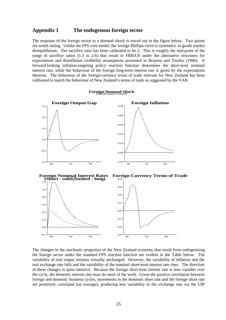
The response of the foreign sector to a demand shock is traced out in the figure below. Two pointsare worth noting. Unlike the FPS core model, the foreign Phillips curve is symmetric in goods marketdisequilibrium. The sacrifice ratio has been calibrated to be 2. This is roughly the mid-point of therange of sacrifice ratios (1.3 to 2.6) that result in FRB/US under the alternative structures forexpectations and disinflation credibility assumptions presented in Brayton and Tinsley (1996). Aforward-looking inflation-targeting policy reaction function determines the short-term nominalinterest rate, while the behaviour of the foreign long-term interest rate is given by the expectationstheorem. The behaviour of the foreign-currency terms of trade relevant for New Zealand has beencalibrated to match the behaviour of New Zealand’s terms of trade as suggested by the VAR.
The changes in the stochastic properties of the New Zealand economy that result from endogenisingthe foreign sector under the standard FPS reaction function are evident in the Table below. Thevariability of real output remains virtually unchanged. However, the variability of inflation and thereal exchange rate falls and the variability of the nominal short-term interest rate rises. The directionof these changes is quite intuitive. Because the foreign short-term interest rate is now variable overthe cycle, the domestic interest rate must do more of the work. Given the positive correlation betweenforeign and domestic business cycles, movements in the domestic short rate and the foreign short rateare positively correlated (on average), producing less variability in the exchange rate via the UIP
26
condition. Additionally, the response of the foreign monetary authority in order to return foreigninflation to control also helps to return domestic inflation to control via import and export prices.
Root Mean Squared Deviations
Output Exchange rate Nominal interestrate
CPI Inflation
Exogenousforeign sector
3.19 5.24 3.59 1.19
Endogenousforeign sector
3.22 4.97 3.89 1.05
27
Appendix 2 Efficient Policy Frontiers
As defined in Taylor (1994), efficient policy rules are those rules that deliver the lowest achievablecombinations of inflation and output variability, given the structure of the model economy underconsideration and the stochastic disturbances applied. In the graph below, the efficient policy frontieris traced out for forward-looking CPI inflation targeting policy rules.25 The two policy rules of thesame class examined in this paper are also shown. These rules lie to the north east of the efficientpolicy frontier. This illustrates that the policy rules examined are not efficient: other policy rulesexist that the monetary authority could use to achieve lower combinations of both output andinflation.
CPI-Y frontier
2.5
3.0
3.5
4.0
4.5
5.0
5.5
0.0 0.2 0.4 0.6 0.8 1.0 1.2 1.4 1.6 1.8 2.0
RMSD CPI Inflation
Frontier: std passthrough, CPI targeting
Std FPS rule
Short FPS rule
The policy rules that lie upon the efficient policy frontier tend to penalise forecast inflation deviationsfrom target far more vigorously than the standard FPS policy rule, or the alternatives presented in thispaper. This is illustrated in the second graph below which shows the trade-off between instrumentand inflation variability. Note that the policy rules presented here all have relatively low instrumentvariability. This finding is common in the extensive literature on policy rules (see Drew and Hunt(1998b)). That is, it is often found that descriptively accurate policy rules, such as the Taylor rule,fare poorly in terms of the inflation/output variability trade-off, but well in terms of instrumentvariability. In other words, policy makers have a high revealed preference for being cautious inadjusting policy. The classic Brainard (1966) article offers a plausible insight into this revealedpreference: if there is also uncertainty about policy multipliers, it may better to act cautiously.
25 See Drew and Hunt (1998b) for a description of the techniques employed to trace out efficient policy frontiers,and a general discussion on the stochastic behaviour of the FPS model under alternative policy rules.