8/3/2019 tarting Simulink
http://slidepdf.com/reader/full/tarting-simulink 1/20
tarting Simulink
Simulink is started from the MATLAB command prompt by entering the following
command:
simulink
Alternatively, you can hit the New Simulink Model button at the top of the
MATLAB command window as shown below:
When it starts, Simulink brings up two windows. The first is the main Simulink
window, which appears as:
The second window is a blank, untitled, model window. This is the window into
which a new model can be drawn.
Model Files
In Simulink, a model is a collection of blocks which, in general, represents a system.
In addition, to drawing a model into a blank model window, previously saved model
files can be loaded either from the File menu or from the MATLAB command prompt.
As an example, download the following model file by clicking on the following link
and saving the file in the directory you are running MATLAB from.
8/3/2019 tarting Simulink
http://slidepdf.com/reader/full/tarting-simulink 2/20
simple.mdl
Open this file in Simulink by entering the following command in the
MATLAB command window. (Alternatively, you can load this file using
the Open option in the File menu in Simulink, or by hitting Ctrl+O in Simulink.) simple
The following model window should appear.
A new model can be created by selecting New from the File menu in any Simulink
window (or by hitting Ctrl+N).
Basic Elements
There are two major classes of items in Simulink: blocks and lines. Blocks are used to
generate, modify, combine, output, and display signals. Lines are used to transfer
signals from one block to another.
Blocks
There are several general classes of blocks:
Sources: Used to generate various signals
Sinks: Used to output or display signals
Discrete: Linear, discrete-time system elements (transfer functions, state-space
models, etc.)
Linear: Linear, continuous-time system elements and connections (summing
junctions, gains, etc.)
Nonlinear: Nonlinear operators (arbitrary functions, saturation, delay, etc.)
Connections: Multiplex, Demultiplex, System Macros, etc.
Blocks have zero to several input terminals and zero to several output terminals.
Unused input terminals are indicated by a small open triangle. Unused output
terminals are indicated by a small triangular point. The block shown below has an
unused input terminal on the left and an unused output terminal on the right.
8/3/2019 tarting Simulink
http://slidepdf.com/reader/full/tarting-simulink 4/20
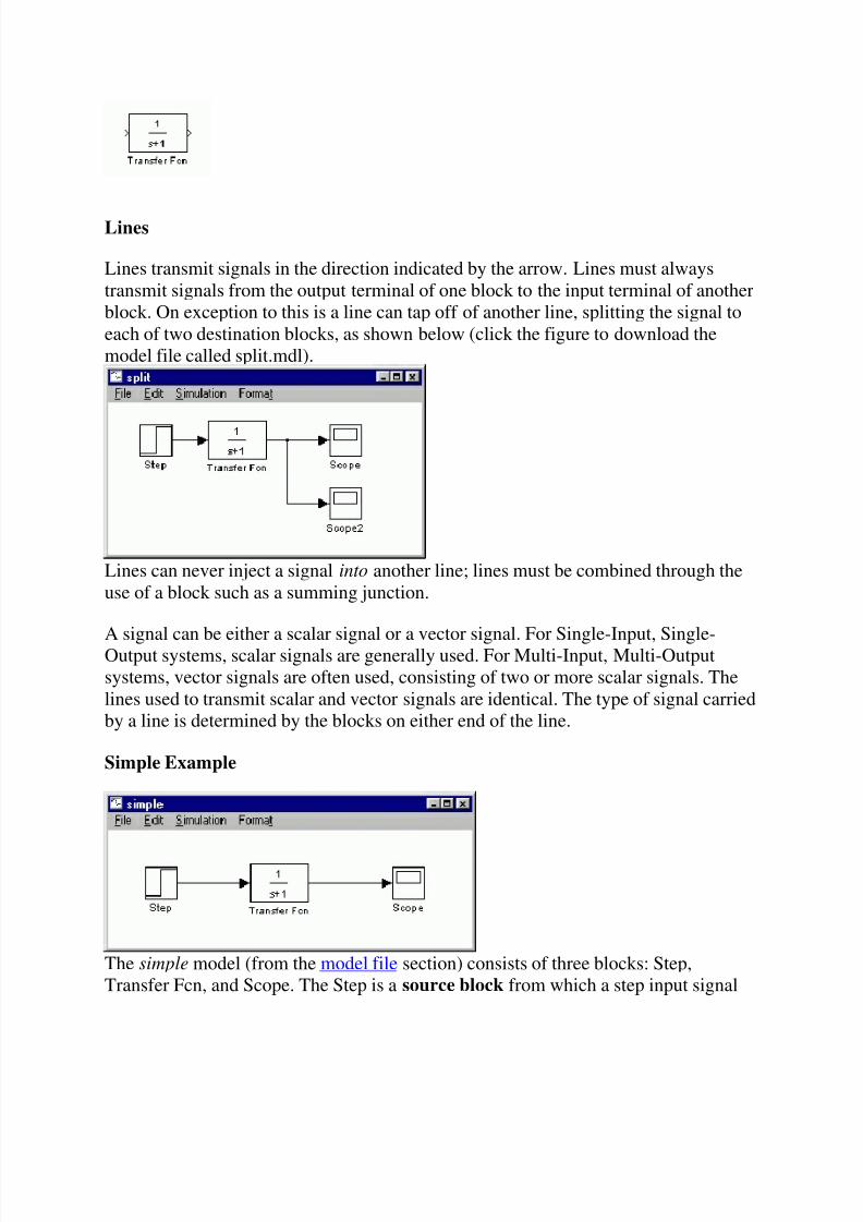
originates. This signal is transfered through the line in the direction indicated by the
arrow to the Transfer Function linear block. The Transfer Function modifies its input
signal and outputs a new signal on a line to the Scope. The Scope is a sink block used
to display a signal much like an oscilloscope.
There are many more types of blocks available in Simulink, some of which will bediscussed later. Right now, we will examine just the three we have used in
the simple model.
Modifying Blocks
A block can be modified by double-clicking on it. For example, if you double-click on
the "Transfer Fcn" block in the simple model, you will see the following dialog box.
This dialog box contains fields for the numerator and the denominator of the block's
transfer function. By entering a vector containing the coefficients of the desired
numerator or denominator polynomial, the desired transfer function can be entered.
For example, to change the denominator to s^2+2s+1, enter the following into the
denominator field: [1 2 1]
and hit the close button, the model window will change to the following,
which reflects the change in the denominator of the transfer function.
8/3/2019 tarting Simulink
http://slidepdf.com/reader/full/tarting-simulink 5/20
The "step" block can also be double-clicked, bringing up the following dialog box.
The default parameters in this dialog box generate a step function occurring at time=1
sec, from an initial level of zero to a level of 1. (in other words, a unit step at t=1).
Each of these parameters can be changed. Close this dialog before continuing.
The most complicated of these three blocks is the "Scope" block. Double clicking on
this brings up a blank oscilloscope screen.
When a simulation is performed, the signal which feeds into the scope will be
displayed in this window. Detailed operation of the scope will not be covered in this
tutorial. The only function we will use is the autoscale button, which appears as a pair
of binoculars in the upper portion of the window.
Running Simulations
To run a simulation, we will work with the following model file:
simple2.mdl
8/3/2019 tarting Simulink
http://slidepdf.com/reader/full/tarting-simulink 6/20
Download and open this file in Simulink following the previous instructions for this
file. You should see the following model window.
Before running a simulation of this system, first open the scope window by double-
clicking on the scope block. Then, to start the simulation, either select Start from
the Simulation menu (as shown below) or hit Ctrl-T in the model window.
The simulation should run very quickly and the scope window will appear as shown
below.
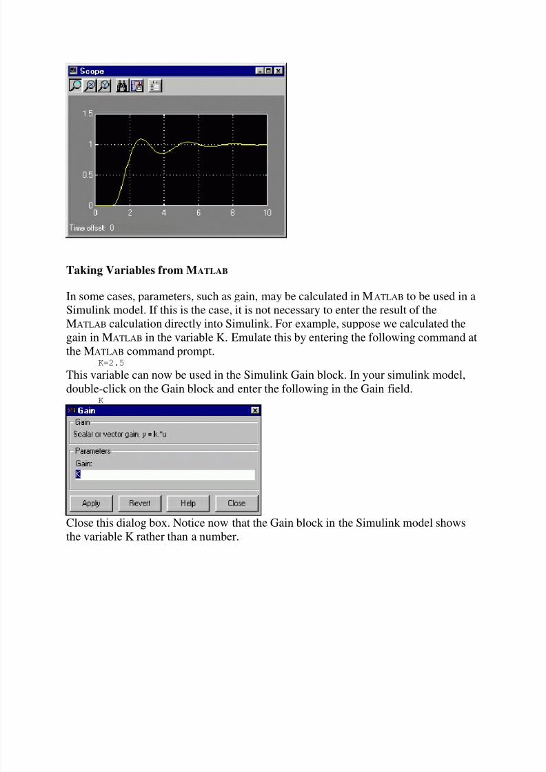
Note that the simulation output (shown in yellow) is at a very low level relative to theaxes of the scope. To fix this, hit the autoscale button (binoculars), which will rescale
the axes as shown below.
8/3/2019 tarting Simulink
http://slidepdf.com/reader/full/tarting-simulink 7/20
Note that the step response does not begin until t=1. This can be changed by double-
clicking on the "step" block. Now, we will change the parameters of the system and
simulate the system again. Double-click on the "Transfer Fcn" block in the modelwindow and change the denominator to
[1 20 400]
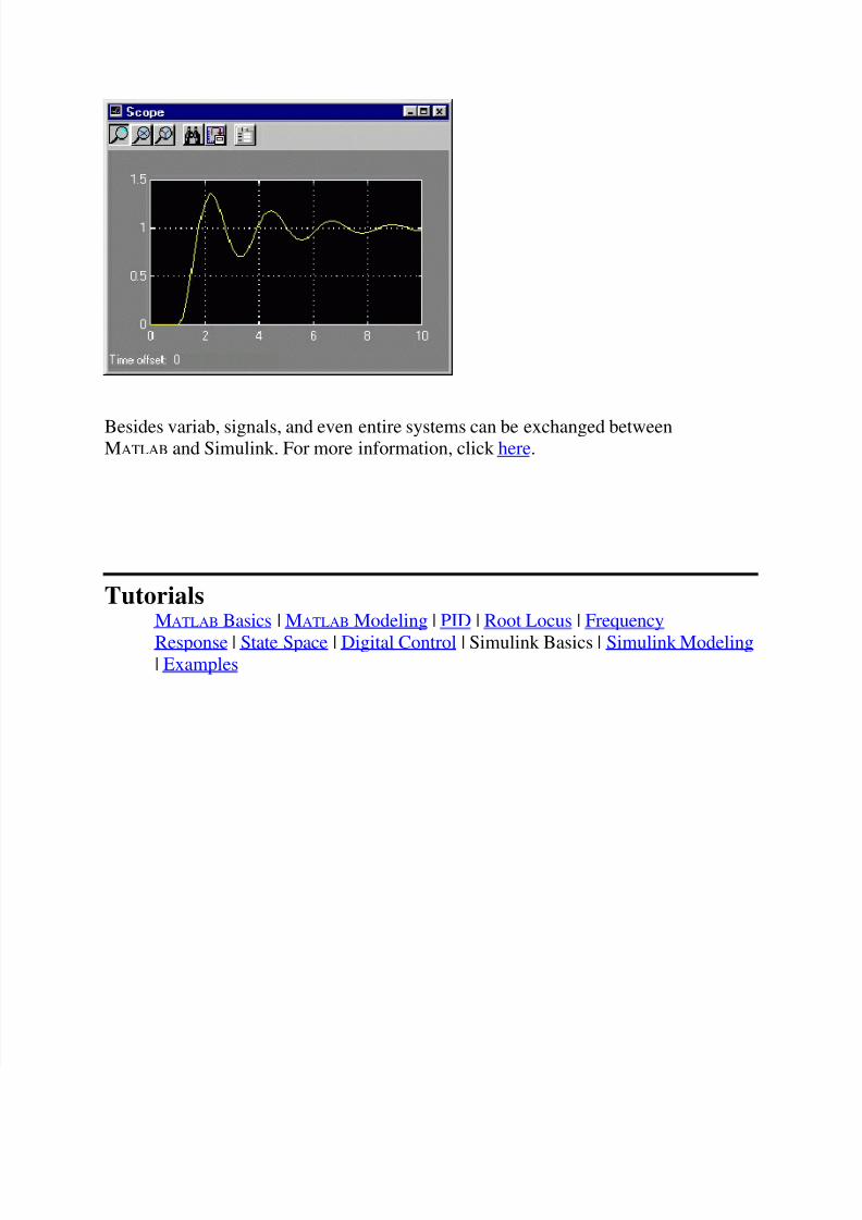
Re-run the simulation (hit Ctrl-T) and you should see what appears as a flat line in the
scope window. Hit the autoscale button, and you should see the following in the scope
window.
Notice that the autoscale button only changes the vertical axis. Since the new transfer
function has a very fast response, it it compressed into a very narrow part of the scopewindow. This is not really a problem with the scope, but with the simulation itself.
Simulink simulated the system for a full ten seconds even though the system had
reached steady state shortly after one second.
To correct this, you need to change the parameters of the simulation itself. In the
model window, select Parameters from the Simulation menu. You will see the
8/3/2019 tarting Simulink
http://slidepdf.com/reader/full/tarting-simulink 8/20
following dialog box.
There are many simulation parameter options; we will only be concerned with the
start and stop times, which tell Simulink over what time period to perform the
simulation. Change Start time from 0.0 to 0.8 (since the step doesn't occur until
t=1.0. Change Stop time from 10.0 to 2.0, which should be only shortly after the
system settles. Close the dialog box and rerun the simulation. After hitting the
autoscale button, the scope window should provide a much better display of the step
response as shown below.
Building Systems
8/3/2019 tarting Simulink
http://slidepdf.com/reader/full/tarting-simulink 9/20
In this section, you will learn how to build systems in Simulink using the building
blocks in Simulink's Block Libraries. You will build the following system.
If you would like to download the completed model, here.
First you will gather all the necessary blocks from the block libraries. Then you will
modify the blocks so they correspond to the blocks in the desired model. Finally, you
will connect the blocks with lines to form the complete system. After this, you will
simulate the complete system to verify that it works.
Gathering Blocks
Follow the steps below to collect the necessary blocks:
Create a new model (New from the File menu or Ctrl-N). You will get a blank
model window.
8/3/2019 tarting Simulink
http://slidepdf.com/reader/full/tarting-simulink 10/20
Double-click on the Sources icon in the main Simulink window.
This opens the Sources window which contains the Sources Block Library.
Sources are used to generate signals. Click here for more information on block
libraries.
8/3/2019 tarting Simulink
http://slidepdf.com/reader/full/tarting-simulink 11/20
Drag the Step block from the sources window into the left side of your model
window.
Double-click on the Linear icon in the main Simulink window to open the
Linear Block Library window. Drag the Sum, Gain, and two instances of the Transfer Fcn (drag it two times)
into your model window arranged approximately as shown below. The exact
alignment is not important since it can be changed later. Just try to get the
correct relative positions. Notice that the second Transfer Function block has a
1 after its name. Since no two blocks may have the same name, Simulink
automatically appends numbers following the names of blocks to differentiate
between them.
Double-click on the Sinks icon in the main Simulink window to open the Sinks
window.
8/3/2019 tarting Simulink
http://slidepdf.com/reader/full/tarting-simulink 12/20
Drag the Scope block into the right side of your model window.
Modify Blocks
Follow these steps to properly modify the blocks in your model.
Double-click your Sum block. Since you will want the second input to be
subtracted, enter +- into the list of signs field. Close the dialog box.
Double-click your Gain block. Change the gain to 2.5 and close the dialog box.
Double-click the leftmost Transfer Function block. Change the numerator to [1
2] and the denominator to [1 0]. Close the dialog box.
Double-click the rightmost Transfer Function block. Leave the numerator [1],
but change the denominator to [1 2 4]. Close the dialog box. Your model
should appear as:
Change the name of the first Transfer Function block by clicking on the words
"Transfer Fcn". A box and an editing cursor will appear on the block's name as
shown below. Use the keyboard (the mouse is also useful) to delete the existing
name and type in the new name, "PI Controller". Click anywhere outside the
8/3/2019 tarting Simulink
http://slidepdf.com/reader/full/tarting-simulink 13/20
name box to finish editing.
Similarly, change the name of the second Transfer Function block from
"Transfer Fcn1" to "Plant". Now, all the blocks are entered properly. Your
model should appear as:
Connecting Blocks with Lines
Now that the blocks are properly laid out, you will now connect them together. Follow
these steps.
Drag the mouse from the output terminal of the Step block to the upper
(positive) input of the Sum block. Let go of the mouse button only when the
mouse is right on the input terminal. Do not worry about the path you followwhile dragging, the line will route itself. You should see the following.
8/3/2019 tarting Simulink
http://slidepdf.com/reader/full/tarting-simulink 14/20
The
resulting line should have a filled arrowhead. If the arrowhead is open, as
shown below, it means it is not connected to anything.
You
can continue the partial line you just drew by treating the open arrowhead as an
output terminal and drawing just as before. Alternatively, if you want to redraw
the line, or if the line connected to the wrong terminal, you should delete the
line and redraw it. To delete a line (or any other object), simply click on it to
select it, and hit the delete key.
Draw a line connecting the Sum block output to the Gain input. Also draw a
line from the Gain to the PI Controller, a line from the PI Controller to the
Plant, and a line from the Plant to the Scope. You should now have the
8/3/2019 tarting Simulink
http://slidepdf.com/reader/full/tarting-simulink 15/20
following.
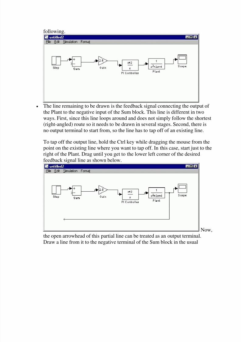
The line remaining to be drawn is the feedback signal connecting the output of
the Plant to the negative input of the Sum block. This line is different in two
ways. First, since this line loops around and does not simply follow the shortest(right-angled) route so it needs to be drawn in several stages. Second, there is
no output terminal to start from, so the line has to tap off of an existing line.
To tap off the output line, hold the Ctrl key while dragging the mouse from the
point on the existing line where you want to tap off. In this case, start just to the
right of the Plant. Drag until you get to the lower left corner of the desired
feedback signal line as shown below.
Now,
the open arrowhead of this partial line can be treated as an output terminal.
Draw a line from it to the negative terminal of the Sum block in the usual
8/3/2019 tarting Simulink
http://slidepdf.com/reader/full/tarting-simulink 16/20
manner.
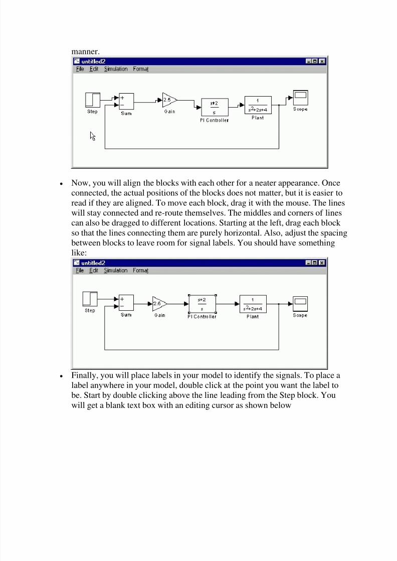
Now, you will align the blocks with each other for a neater appearance. Once
connected, the actual positions of the blocks does not matter, but it is easier toread if they are aligned. To move each block, drag it with the mouse. The lines
will stay connected and re-route themselves. The middles and corners of lines
can also be dragged to different locations. Starting at the left, drag each block
so that the lines connecting them are purely horizontal. Also, adjust the spacing
between blocks to leave room for signal labels. You should have something
like:
Finally, you will place labels in your model to identify the signals. To place a
label anywhere in your model, double click at the point you want the label to
be. Start by double clicking above the line leading from the Step block. Youwill get a blank text box with an editing cursor as shown below
8/3/2019 tarting Simulink
http://slidepdf.com/reader/full/tarting-simulink 17/20
Type
an r in this box, labeling the reference signal and click outside it to end editing.
Label the error (e) signal, the control (u) signal, and the output (y) signal in the
same manner. Your final model should appear as:
To save your model, select Save As in the File menu and type in any desired
model name. The completed model can be found here.
Simulation
Now that the model is complete, you can simulate the model. Select Start from
the Simulation menu to run the simulation. Double-click on the Scope block to view
its output. Hit the autoscale button (binoculars) and you should see the following.
8/3/2019 tarting Simulink
http://slidepdf.com/reader/full/tarting-simulink 18/20
Taking Variables from MATLAB
In some cases, parameters, such as gain, may be calculated in MATLAB to be used in a
Simulink model. If this is the case, it is not necessary to enter the result of the
MATLAB calculation directly into Simulink. For example, suppose we calculated the
gain in MATLAB in the variable K. Emulate this by entering the following command at
the MATLAB command prompt. K=2.5
This variable can now be used in the Simulink Gain block. In your simulink model,
double-click on the Gain block and enter the following in the Gain field. K
Close this dialog box. Notice now that the Gain block in the Simulink model shows
the variable K rather than a number.
8/3/2019 tarting Simulink
http://slidepdf.com/reader/full/tarting-simulink 20/20
Besides variab, signals, and even entire systems can be exchanged betweenMATLAB and Simulink. For more information, click here.
Tutorials
MATLAB Basics | MATLAB Modeling | PID | Root Locus | Frequency
Response | State Space | Digital Control | Simulink Basics | Simulink Modeling | Examples