Tasche_2009

8/13/2019 Tasche_2009

http://slidepdf.com/reader/full/tasche2009 1/58

Estimating discriminatory power and PD curves when the

number of defaults is small

Dirk Tasche, Lloyds Banking Group∗

Abstract

The intention with this paper is to provide all the estimation concepts and techniques thatare needed to implement a two-phases approach to the parametric estimation of probability

of default (PD) curves. In the first phase of this approach, a raw PD curve is estimated basedon parameters that reflect discriminatory power. In the second phase of the approach, theraw PD curve is calibrated to fit a target unconditional PD. The concepts and techniquespresented include a discussion of different definitions of area under the curve (AUC) andaccuracy ratio (AR), a simulation study on the performance of confidence interval estima-tors for AUC, a discussion of the one-parametric approach to the estimation of PD curvesby van der Burgt (2008) and alternative approaches, as well as a simulation study on theperformance of the presented PD curve estimators. The topics are treated in depth in orderto provide the full rationale behind them and to produce results that can be implementedimmediately.

1 Introduction

In the current economic environment with its particular consequence of rising credit default ratesall over the world, at first glance it might not seem very appropriate to look after estimationissues experienced in portfolios with a small number of defaults. However, low default estimationissues can occur quite naturally even in such a situation:

• It is of interest to estimate instantaneous discriminatory power of a score function orrating system. “Instantaneous” means that one looks only at the defaults and survivalsthat occurred in a relatively short time period as one year or less. In typical wholesaleportfolios that represent the scope of a rating system the number of borrowers does notexceed 1000. As a consequence, the number of defaults observed within a one year periodmight well be less than 20.

• Similarly, when estimating forward-looking point-in-time (PIT) conditional probabilitiesof default per score or rating grade (PD curve), it makes sense to construct the estimationsample from observations in a relatively short time period like one or two years in order tocapture the instantaneous properties of a potentially rather volatile object. The previousobservation on the potentially low number of defaults then applies again.

∗The opinions expressed in this paper are those of the author and do not necessarily reflect views of LloydsBanking Group.

1

a r X

i v : 0 9 0 5 . 3 9 2 8 v 2 [ q - f i n . R M ] 5 M a r 2 0 1 0

8/13/2019 Tasche_2009


8/13/2019 Tasche_2009


questions of how the power of such score functions or rating systems can be assessed and howprobability of default (PD) estimates (PD curves) associated with score values or rating gradescan be derived.

In sub-section 2.1 we present a general concept for the calibration of score functions and rating

systems which is based on separate estimation of discriminatory power and an unconditionalprobability of default. In sub-section 2.2 a simple probabilistic model is introduced that will helpin the derivation of some ideas and formulas needed for implementation of the concept. Moreover,in sub-section 2.3 we recall for further reference some properties of distribution functions andsome notation related to such functions.

2.1 Estimation phase and calibration phase

In this sub-section, we introduce the concept of a two-phases approach to the calibration of ascore function or a rating system: The first phase is the estimation phase, the second phase is

the calibration and forecast phase.

2.1.1 Estimation

The aim here is to estimate conditional PDs per score (or grade) and the discriminatory power of the rating system (to be formally defined in sections 3 and 3.2) from a historical sample of scoresor rating grades associated with borrowers whose solvency states one period after the scores wereobserved are known. The composition of the sample is not assumed to be representative of currentor future portfolio composition. In particular, the proportion of defaulters and survivors in thesample may differ from proportions of defaulters and survivors expected for the future. Theestimated conditional PDs therefore are considered raw PDs and have to be calibrated beforebeing further used. The estimation sample could be the development sample of the rating systemor a validation sample.

In the following, we will write x1, . . . , xnD when talking about a sample of scores or rating gradesof defaulted borrowers and y1, . . . , ynN when talking about a sample of surviving borrowers. Inboth these cases, the solvency state of the borrowers one period after the observation of thescores is known. In contrast, we will write s1, . . . , sn when talking about a sample of scores of borrowers with unknown future solvency state.

2.1.2 Calibration and forecast

The aim here is to calibrate the raw PDs from the estimation step in such a way that, on thecurrent portfolio, they are consistent with an unconditional PD that may be different to theunconditional PD of the estimation sample. This calibration exercise is needed because for theborrowers in the current portfolio scores (or rating grades) can be determined but not theirfuture solvency states. Hence direct estimation of conditional PDs with the current portfolio assample is not possible. We will provide the details of the calibration under the assumption thatthe conditional score distributions (formally defined in (2.3) below) that underlie the estima-tion sample and the conditional score distributions of the current portfolio are the same. Thisassumption is reasonable if the estimation sample was constructed not too far back in time or if

3

8/13/2019 Tasche_2009


the rating system was designed with an intention of creating a through-the-cycle (TTC) ratingsystem.

As mentioned before, the unconditional PDs of estimation sample and current portfolio may bedifferent. This will be the case in particular if a point-in-time (PIT) calibration of the conditional

PDs is intended, such that the PDs can be used for forecasting future default rates. But also if aTTC calibration of the PDs is intended (such that no direct forecast of default rates is possible),most of the time the TTC unconditional PD will be different to the realised unconditional PDof the estimation sample. Note that the unconditional score distributions of estimation sampleand current portfolio can be different but, on principle, are linked together by equation (2.4)from sub-section 2.2.

The question of how to forecast the unconditional PD is not treated in this paper. An exampleof how PIT estimation of the unconditional PD could be conducted is presented by Engelmannand Porath (2003, section III). Technical details of how the calibration of the conditional PDscan be done are provided in appendix A.

2.2 Model and basic properties

Speaking in technical terms, in this paper we study the joint distribution and some estimationaspects of a pair (S, Z ) of real random variables. The variable S is interpreted as the credit score (continuous case) or rating grade 1 (discrete case) observed for a solvent borrower at a certainpoint in time. Hence S typically takes on values on a continuous scale in some open intervalI ⊂ R or on a discrete scale in a finite set I = {1, 2, . . . , k}.

Convention: Low values of S indicate low creditworthiness (“bad”), high values of S indicatehigh creditworthiness (“good”).

The variable Z is the borrower’s state of solvency one observation period (usually one year)after the score was observed. Z takes on values in {0, 1}. The meaning of Z = 0 is “borrowerhas remained solvent” (solvency or survival), Z = 1 means “borrower has become insolvent”(default). We write D for the event {Z = 1} and N for the event {Z = 0}. Hence

D ∩ N = {Z = 1} ∩ {Z = 0} = ∅, D ∪ N = whole space. (2.1)

The marginal distribution of the state variable Z is characterised by the unconditional probability of default p which is defined as

p = P[D] = P[Z = 1] ∈ [0, 1]. (2.2)

The joint distribution of (S, Z ) then can be specified by the two conditional distributions of S

given the states of Z or the events D and N respectively. In particular, we define the conditionaldistribution functions

F N (s) = P[S ≤ s | N ] = P[{S ≤ s} ∩ N ]

1 − p , s ∈ I,

F D(s) = P[S ≤ s | D] = P[{S ≤ s} ∩ D]

p , s ∈ I.

(2.3)

1In practice, often a rating system with a small finite number of grades is derived from a score functionwith values on a continuous scale. This is usually done by mapping score intervals on rating grades. See Tasche(2008, section 3) for a discussion of how such mappings can be defined. Discrete rating systems are preferredby practitioners because manual adjustment of results (overrides) is feasible. Moreover, results by discrete ratingsystems tend to be more stable over time.

4

8/13/2019 Tasche_2009


For the sake of an easier notation we denote by S N and S D random variables with distributionsP[S ∈ · | N ] and P[S ∈ · | D] respectively. In the literature, F N (s) sometimes is called false alarm rate while F D(s) is called hit rate .

By the law of total probability, the distribution function F (s) = P[S

≤ s] of the marginal (or

unconditional) distribution of the score S can be represented as

F (s) = p F D(s) + (1 − p) F N (s), all s. (2.4)

F (s) is often called alarm rate .

The joint distribution of the pair (S, Z ) of score and borrower’s state one period later can also bespecified by starting with the unconditional distribution P[S ∈ · ] of S and combining it with theconditional probability of default P[D | S ] = 1 − P[N | S ]. Recall that in general the conditionalprobability P[D | S ] = pD(S ) can be characterised2 by the property (see, e.g. Durrett, 1995,section 4.1)

E[ pD(S ) 1{S ∈A}] = P [D

∩ {S

∈A

}], (2.5)

for all Borel sets A ⊂ R. It is well-known (Bayes’ formula) that equation (2.5) implies closed-formrepresentations of P[D | S = s] = pD(s) in two important special cases:

• S is a discrete variable, i.e. S ∈ I = {1, 2, . . . , k}. Then

P[D | S = j ] = p P[S = j | D]

p P[S = j | D] + (1 − p) P[S = j | N ] , j ∈ I. (2.6a)

• S is a continuous variable with values in an open interval I such that there are Lebesguedensities f N and f D of the conditional distribution functions F N and F D from (2.3). Then

P[D | S = s] = p f D(s) p f D(s) + (1 − p) f N (s)

, s ∈ I. (2.6b)

A closely related consequence of equation (2.5) is the fact that p, F N , and F D can be determinedwhenever the unconditional score distribution F and the conditional probabilities of defaultP[D | S ] are known. We then obtain

p = E

P[D | S ]

=

k j=1 P[D | S = j ] P[S = j ], S discrete I P[D | S = s] f (s) ds, S continuous with density f .

(2.7a)

If S is a discrete rating variable, we have for j ∈ I

P[S = j | D] = P[D | S = j ] P[S = j ]/p,

P[S = j | N ] =

1 − P[D | S = j ]

P[S = j ]/(1 − p).(2.7b)

If S is continuous score variable with density f , we have for s ∈ I

f D(s) = P[D | S = s] f (s)/p,

f N (s) =

1 − P[D | S = s]

f (s)/(1 − p).(2.7c)

2We define the indicator function 1M of a set M by 1M (m) =

1, m ∈ M,

0, m /∈ M.

5

8/13/2019 Tasche_2009


2.3 Notation for distribution functions

At some points in this paper we will need to handle distribution functions and their inverse func-tions. For further reference we list in this subsection the necessary notation and some properties

of such functions:

• A (real) distribution function G is an increasing and right-continuous function R→ [0, 1]with lim

x→−∞G(x) = 0 and lim

x→∞G(x) = 1.

• Any real random variable X defines a distribution function G = GX by G(x) = P[X ≤ x].

• Convention: G(−∞) = 0 and G(∞) = 1.

• Denote by G(· − 0) the left-continuous version of the distribution function G. Then G(· −0) ≤ G and G(x − 0) = G(x) for all x but countably many x ∈ R because G is non-decreasing.

• For any distribution function G, the function G−1 is its generalised inverse or quantile function , i.e.

G−1(u) = inf {x ∈ R : G(x) ≥ u}, u ∈ [0, 1]. (2.8a)

In particular, we obtain− ∞ = G−1(0) < G−1(1) ≤ ∞. (2.8b)

• Denote by ϕ(s) the standard normal density and by Φ(s) the standard normal distributionfunction.

3 Discriminatory power: Theory

Hand (1997, section 8.1) described ROC curves as follows: “Often the two degrees of freedom[i.e. the two error types associated with binary classification] are presented simultaneously for arange of possible classification thresholds for the classifier in a receiver operating characteristic (ROC) curve . This is done by plotting true positive rate (sensitivity) on the vertical axis againstfalse positive rate (1 - specificity) on the horizontal axis.”

Translated into the notation introduced in section 2, for a fixed score value s seen as threshold thetrue positive rate is the hit rate F D(s) while the false positive rate is the false alarm rate F N (s).In these terms, CAP (Cumulative Accuracy Profile) curves (not mentioned by Hand, 1997) canbe described as a plot of the hit rates against the alarm rates across a range of classification

thresholds. If all possible thresholds are to be considered, these descriptions formally can beexpressed in the following terms.

Definition 3.1 (ROC and CAP) Denote by F N the distribution function F N (s) = P[S N ≤s] of the scores conditional on the event “borrower survives”, by F D the distribution function F D(s) = P[S D ≤ s] of the scores conditional on the event “borrower defaults”, and by F the unconditional distribution function F (s) = P[S ≤ s] of the scores.

The Receiver Operating Characteristic (ROC) of the score function then is defined as the graph of the following set gROC (“g” for graph) of points in the unit square:

gROC = F N (s), F D(s) : s ∈ R ∪{±∞}. (3.1a)

6

8/13/2019 Tasche_2009


The Cumulative Accuracy Profile (AUC) of the score function is defined as the graph of the following set gCAP of points in the unit square:

gCAP =

F (s), F D(s)

: s ∈ R ∪{±∞}

. (3.1b)

Actually the point sets gROC and gCAP can be quite irregular (e.g. if one of the involveddistribution functions has an infinite number of discontinuities and the set of discontinuities isdense in R). In such a case it would be physically impossible to plot on paper a precise graphof the point set. In most parts of the following, therefore, we will focus on three more regularspecial cases which are of relevance for theory and practice:

1) F , F N , and F D are smooth, i.e. at least continuous. This is usually a reasonable assumptionwhen the score function takes on values on a continuous scale.

2) The distributions of S , S N and S D are concentrated on a finite number of points. Thisis the case when the score function is a rating system with a finite number (e.g. seven or

seventeen as in case of S & P, Moody’s, or Fitch ratings) of grades.

3) F , F N , and F D are empirical distribution functions associated to finite samples of scoreson a continuous scale. This is naturally the case when the performance of a score functionis analysed on the basis of non-parametric estimates.

In the smooth situation of 1) the sets gROC and gCAP are compact and connected such thatthere is no ambiguity left of how to draw a graph that – together with the x-axis and the verticalline through x = 1 – encloses a region of finite area. In situations 2) and 3), however, the setsgROC and gCAP consist of a finite number of isolated points and hence are unconnected. Whilethis, in a certain sense, even facilitates the drawing of the graphs, the results nonetheless will be

unsatisfactory when it comes to a comparison of the discriminatory power of score functions orrating systems. Usually, therefore, in such cases a certain degree of interpolation will be appliedto the points of the sets gROC and gCAP in order to facilitate their visual comparison. We willdiscuss in section 3.2 the question of how to do best the interpolation to satisfy some propertiesthat are desirable from a statistical point of view.

Before, however, in section 3.1 we have a closer look on the properties of ROC graphs in smoothcontexts. These properties then will be used as a kind of yardstick to assess the appropriatenessof interpolation approaches to the discontinuous case in section 3.2.

3.1 Continuous score distributions

In this subsection, we will work most of the time on the basis of one of the following twoassumptions.

Assumption N: The distribution of the score S N conditional on the borrower’s survival iscontinuous, i.e.

P[S N = s] = 0 for all s. (3.2)

Assumption S: The unconditional distribution of the score S is continuous (and hence by (2.4)so are the distributions of S N and S D), i.e.

P[S = s] = 0 for all s. (3.3)

7

8/13/2019 Tasche_2009


Additionally, the following technical assumption is sometimes useful.

Assumption:F −1D (1) ≤ F −1N (1). (3.4)

This is equivalent to requiring that the essential supremum of S D

is not greater than the essen-tial supremum of S N . Such a requirement seems natural under the assumption that low scorevalues indicate low creditworthiness (“bad”) and high score values indicate high creditworthiness(“good”).

As an immediate consequence of these assumptions we obtain representations of the ROC andCAP sets (3.1a) and (3.1b) that are more convenient for calculations.

Theorem 3.2 (Standard parametrisations of ROC and CAP)With the notation of definition 3.1 define the functions ROC and CAP by

ROC(u) = F DF −1N (u), u ∈ [0, 1], (3.5a)

CAP(u) = F DF −1(u) = F D( p F D(·) + (1 − p) F N (·))−1(u), u ∈ [0, 1]. (3.5b)

For (3.5b), assume p > 0 (otherwise ROC and CAP coincide). Under (3.2) (assumption N)then we have

u, ROC(u)

: u ∈ [0, 1] ⊂ gROC. (3.5c)

If under (3.2) (assumption N), moreover, the distribution of S D is absolutely continuous with respect to the distribution of S N (i.e. P[S N ∈ A] = 0 ⇒ P[S D ∈ A] = 0), then 3 “ =” applies also to (3.5c):

u, ROC(u)

: u ∈ [0, 1]

= gROC. (3.5d)

Equation (3.3) (assumption S) implies u, CAP(u) : u ∈ [0, 1] = gCAP. (3.5e)

Proof. Note that (2.8b) implies in general

0 = CAP(0) = ROC(0). (3.6a)

For p > 0, we have

s : p F D(s) + (1 − p) F N (s) ≥ 1 ⊂ s : F D(s) ≥ 1

and hence

CAP(1) = F D

( p F D(·) + (1 − p) F N (·))−1(1)

≥ F D

F −1D (1)

≥ 1⇒ CAP(1) = 1. (3.6b)

Additionally, if (3.4) holds – which is implied by the absolute continuity assumption – we obtain

ROC(1) = F D

F −1N (1)

≥ F D

F −1D (1)

≥ 1

⇒ ROC(1) = 1. (3.6c)

3The absolute continuity requirement implies that F D is constant on the intervals on which F N is constant.

8

8/13/2019 Tasche_2009


Now, by (3.2) (assumption N) we have F N

F −1N (u)

= u and by (3.3) (assumption S) we haveF

F −1(u)

= u (see van der Vaart, 1998, section 21.1). This implies (3.5c) and “⊂” in (3.5e).Assume that distribution of S D is absolutely continuous with respect to the distribution of S N .For s ∈ R let s0 = F −1N

F N (s)

. By continuity of F N then we have F N (s0) = F N (s), and by

absolute continuity of S D

with respect to S N

we also have F D

(s0

) = F D

(s). This implies “=”in (3.5c) because on the one hand

F N (s), F D(s)

=

F N (s), F D(s0)

=

F N (s), ROC

F N (s) ∈ u, ROC(u)

: u ∈ [0, 1]

,

and on the other hand for s = ±∞ we can apply (3.6a), (3.6b), and (3.6c).The “=” in (3.5e) follows from the fact that S D by (2.4) is always absolutely continuous withrespect to S .

Remark 3.3A closer analysis of the proof of theorem 3.2 shows that a non-empty difference between the left-hand and the right-hand sides of (3.5c) can occur only if there are non-empty intervals on which the value of F N is constant. To each such interval on which F D is not constant there is corresponding piece of a vertical line in the set gROC that has no counterpart in the graph of the function ROC(u). Note, however, that these missing pieces are not relevant with respect to the area below the ROC curve because this area is still well-defined when all vertical pieces are removed from gROC. In this sense, in theorem 3.2 the absolute continuity requirement and equation (3.5d) are only of secondary importance.

In view of theorem 3.2 and remark 3.3, we can regard ROC and CAP curves as graphs forfunctions (3.5a) and (3.5b) respectively, as long as (3.2) and (3.3) apply. This provides a conve-nient way to dealing analytically with ROC and CAP curves. In section 3.2 we will revisit thequestion of how to conveniently parametrize the point sets (3.1a) and (3.1b) in the case of scoredistributions with discontinuities.

In this section, we continue by looking closer at some well-known properties of ROC and CAPcurves. In non-technical terms the following proposition 3.4 states: The diagonal line is the ROCand CAP curve of powerless rating systems (or score functions). For a perfect score function,the ROC curve is essentially the horizontal line at level 1 while the CAP curve is made up bythe straight line u → u/p,u < p and the horizontal line at level 1.

Proposition 3.4 Under (3.2) (assumption N), in case of a powerless classification system (i.e.F D = F N ) we have

ROC(u) = u = CAP(u), u ∈ [0, 1]. (3.7a)

In case of a perfect classification system 4 (i.e. there is a score value s0 such that F D(s0) =

1, F N (s0) = 0) we obtain without continuity assumption that

ROC(u) =

0, u = 0,

1, 0 < u ≤ 1,(3.7b)

and, if p > 0 and F D is continuous,

CAP(u) =

u/p, 0 ≤ u < p,

1, p ≤ u ≤ 1.(3.7c)

4Note that in case of a perfect classification system the distribution of S D is not absolutely continuous withrespect to the distribution of S N as it would be required for (3.5d) to obtain.

9

8/13/2019 Tasche_2009


Proof. For (3.7a), we have to show that

F D

F −1D (u)

= u, u ∈ [0, 1]. (3.8)

This follows from the continuity assumption (3.2) (see van der Vaart, 1998, section 21.1).

On (3.7b) and (3.7c): Observe that F D(s0) = 1, F N (s0) = 0 for some s0 implies (3.4). By (3.6a),(3.6b) and (3.6c), therefore, we only need to consider the case 0 < u < 1. For u > p we obtain

F (s0) = p F D(s0) + (1 − p) F N (s0) = p (3.9)

⇒ F −1(u) ≥ s0

⇒ F D

F −1(u)

= 1.

This implies (3.7b) (with p = 0), in particular, and (3.7c) for u > p. For u < p, equation (3.9)implies F −1(u) < s0. By left continuity of F −1, we additionally obtain F −1(u) ≤ s0 for u ≤ p.But

F (s) = p F D(s) + (1−

p) F N (s) = p F D(s), s≤

s0.

Hence for u ≤ p

F −1(u) = inf {s : p F D(s) ≥ u} = F −1D (u/p)

⇒ F D

F −1(u)

= F D

F −1D (u/p)

= u/p.

The last equality follows from the assumed continuity of F D.

By theorem 3.2, in the continuous case (3.2) and (3.3), the common notions of AUC (area underthe curve) and AR (accuracy ratio) can be defined in terms of integrals of the ROC and CAPfunctions (3.5a) and (3.5b). Recall that the accuracy ratio commonly is described in terms likethese: “The quality of a rating system is measured by the accuracy ratio AR. It is defined as

the ratio of the area between the CAP of the rating model being validated and the CAP of therandom model [= powerless model], and the area between the CAP of the perfect rating modeland the CAP of the random model” (Engelmann et al., 2003a, page 82).

Definition 3.5 (Area under the curve and accuracy ratio)For the function ROC given by (3.5a) we define the area under the curve AUC by

AUC =

10

ROC(u) du. (3.10a)

For the function CAP given by (3.5b) we define the accuracy ratio AR by

AR = 10 CAP(u) − u du

1 − p/2 − 1/2 =

2 10 CAP(u) du − 1

1 − p . (3.10b)

In the continuous case (3.3) (assumption S) AUC and AR are identical up to a constant lineartransformation, as shown by the following proposition.

Proposition 3.6 (AUC and AR in the continuous case)If the distribution of the score function conditional on default is continuous then

AR = 2 AUC − 1.

10

8/13/2019 Tasche_2009


Proof. Denote by S D a random variable with the same distribution F D as S D but independent of S D. Let S N be independent of S D. Observe that F −1N (U ) and F −1D (U ) have the same distributionas S N and S D if U is uniformly distributed on (0, 1). By the definition (3.10b) of AR and Fubini’stheorem, therefore we obtain

AR = 21 − p

p P[S D ≤ S D] + (1 − p) P[S D ≤ S N ] − 1/2 (3.11)

= 2 P[S D ≤ S N ] − 1

= 2 AUC − 1.

In this calculation, the fact has been used that 1/2 = P[S D ≤ S D] because the distribution of S D is assumed to be continuous.

As the ROC curve does not depend on the proportion p of defaulters in the population, propo-sition 3.6 in particular shows that AR does not depend on p either. The following corollary isan easy consequence of propositions 3.4 and 3.6. It identifies the extreme cases for classification

systems. A classification system is considered poor if its AUC and AR are close to AUC and ARof a powerless system. It is considered powerful if if its AUC and AR are close to AUC and ARof a perfect system.

Corollary 3.7 Under (3.2) (assumption N), in case of a powerless classification system (i.e.F D = F N ) we have

AUC = 1/2,

AR = 0.(3.12a)

In case of a perfect classification system (i.e. there is a score value s0 such that F D(s0) =

1, F N (s0) = 0) we obtain if the distribution of the scores conditional on default is continuous

AUC = 1,

AR = 1.(3.12b)

Relation (3.12a) can obtain also in situations where F N = F D. For instance, Clavero Rasero(2006, proposition 2.6) proved that (3.12a) applies in general when F N and F D have densitiesthat are both symmetric with respect to the same point.

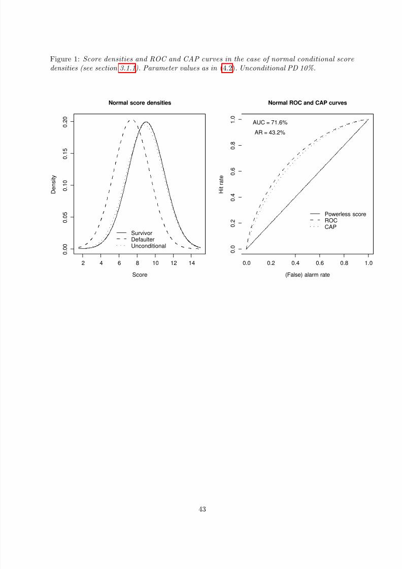
3.1.1 Example: Normally distributed scores

Assume that the score distributions conditional on default and survival, respectively, are normal:

S D ∼ N (µD, σ2D), S N ∼ N (µN , σ2N ). (3.13)

Formulas for ROC in the sense of (3.5a) and AUC in the sense of (3.10a) then easily are derived:

ROC(u) = ΦσN Φ

−1(u) + µN − µDσD

, u ∈ [0, 1]

AUC = Φ

µN − µD

σ2N + σ2D

.

(3.14)

11

8/13/2019 Tasche_2009


Note that (3.14) gives a closed form of AUC where Satchell and Xia (2008) provided a formulainvolving integration. See figure 1 for an illustration of (3.13) and (3.14).

The unconditional score distribution F can be derived from (2.4). Under (3.13), however, for p /

∈ {0, 1

}, F is not a normal distribution function. Its inverse function F −1 can be evaluated

numerically, but no closed-form representation is known. For plots of the CAP curve, thereforeit is more efficient to make use of representation (3.1b). The value of AR can be derived fromthe value of AUC by proposition 3.6.

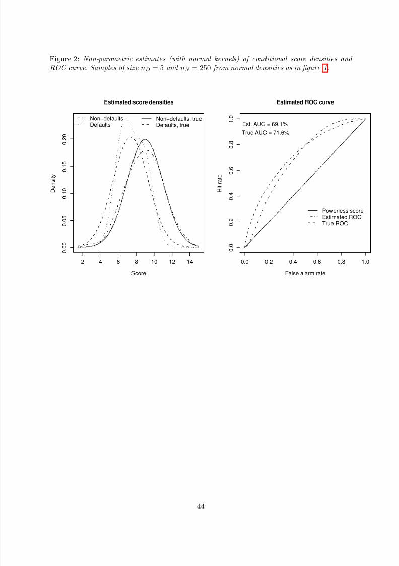
3.1.2 Example: Density estimation with normal kernel

Assume that there are samples x1, . . . , xnD of scores of defaulted borrowers and y1, . . . , ynN of surviving borrowers. If the scores take on values on a continuous scale, it makes sense to try andestimate densities of the defaulters’ scores and survivors’ scores, respectively. We consider herekernel estimation with a normal kernel as estimation approach (see, e.g. Pagan and Ullah, 1999,

chapter 2). The resulting density estimates then are

f D(s) = (nD hD)−1nDi=1

ϕs − xi

hD

,

f N (s) = (nN hN )−1

nN i=1

ϕs − yi

hN

,

(3.15)

where hD, hN > 0 denote appropriately selected bandwidths . Silverman’s rule of thumb (see, e.g.Pagan and Ullah, 1999, equation (2.50)) often yields reasonable results:

h = 1.06 σ T −1/5, (3.16)

where σ denotes the standard deviation of the sample x1, . . . , xnD or y1, . . . , ynN , respectively.Equation (3.15) immediately implies the following formulas for the corresponding estimateddistribution functions:

F D(s) = (nD)−1nDi=1

Φs − xi

hD

,

F N (s) = (nN )−1

nN i=1

Φs − yi

hN

.

(3.17)

ROC and CAP curves then can be drawn efficiently by taking recourse to (3.1a) and (3.1b). Anestimate of AUC (and then by proposition 3.6 of AR) is given by a generalisation of (3.14):

AU C = (nD nN )−1

nDi=1

nN j=1

Φ y j − xi

h2N + h2D

. (3.18)

See figure 2 for illustration.

Remark 3.8 (Bias of kernel-based AUC-estimator)Assume that the samples x1, . . . , xnD of scores of defaulted borrowers and y1, . . . , ynN of scores

12

8/13/2019 Tasche_2009


of surviving borrowers are samples from normally distributed score functions as in (3.13). Then

the expected value of the AUC-estimator AU C from (3.18) can be calculated as follows:

E

AU C

= Φ

µN − µD

h2N + h2D + σ2N + σ2D

.

Hence by (3.14), the following observations apply:E AU C − 1/2

≤ |AUC − 1/2|sign

E AU C

− 1/2

= sign(AUC − 1/2)

µD = µN ⇔ E AU C

= AUC

µD = µN ⇔ A U C = 1/2.

In particular, in case µN > µD the estimator AU C on average underestimates the area under

the curve while in case µN < µD the area under the curve is overestimated by

AU C .

To account for the potential bias of the AUC estimates by (3.18) as observed in remark 3.8,in section 4 we will apply linear transformations to the density estimates (3.15). These lineartransformations make sure that the means and variances of the estimated densities exactlymatch the empirical means and variances of the samples x1, . . . , xnD and y1, . . . , ynN respectively(Davison and Hinkley, 1997, section 3.4). Define

bD =

1/nnD

i=1 x2i − (1/n

nDi=1 xi)2

h2D + 1/n

nDi=1 x2i − (1/n

nDi=1 xi)2

, aD = 1 − bD

n

nDi=1

xi, (3.19a)

bN =

1/nnN j=1 y2 j − 1/nnN

j=1 y j2

h2N + 1/nnN

j=1 y2 j −

1/nnN

j=1 y j

2 , aN = 1 − bN

n

nN j=1

y j. (3.19b)

Replace then in equations (3.15), (3.17), and (3.18)

xi by aD + bD xi and hD by bD hD,

y j by aN + bN y j and hN by bN hN ,(3.19c)

to reduce the bias from an application of (3.18) for AUC estimation. If, for instance, in theright-hand panel of figure 2 the estimated ROC curve is based on the transformed samples

according to (3.19c), the resulting estimate of AUC is 71.2%. Thus, at least in this example, the“transformed” AUC estimate is closer to the true value of 71.6% than the estimate based onestimated densities without adjustments for mean and variance.

3.2 Discontinuous score distributions

We have seen that in the case of continuous score distributions as considered in section 3.1 thereare standard representations of ROC and CAP curves (theorem 3.2) that can be convenientlydeployed to formally define the area under the curve (AUC) and the accuracy ratio (AR) andto investigate some of their properties. In this section, we will see that in a more general setting

13

8/13/2019 Tasche_2009


the use of the curve representations (3.5a) and (3.5b) can have counter-intuitive implications.We then will look at modifications of (3.5a) and (3.5b) that avoid such implications and showthat these modifications are compatible with common interpolation approaches to the ROC andCAP graphs as given by (3.1a) and (3.1b). We will do so primarily with a view on the settingsdescribed in items 2) and 3) at the beginning of section 3. For the sake of reference, the followingtwo examples describe these settings in more detail.

Example 3.9 (Rating distributions)Consider a rating system with grades 1, 2, . . . , n where n stands for highest creditworthiness.The random variable R which expresses a borrower’s rating grade then is purely discontinuousbecause

P[R = k] ≥ 0, k ∈ {1, 2, . . . , n}P[R /∈ {1, 2, . . . , n}] = 0.

See the upper panel of figure 3 for illustration. As in the case of score functions S , we write RD when considering R on the sub-population of defaulters and RN when considering R on the sub-population of survivors.

Example 3.10 (Sample-based empirical distributions)Assume – as in section 3.1.2 – that there are samples x1, . . . , xnD of scores of defaulted borrow-ers and y1, . . . , ynN of surviving borrowers. If there is no reason to believe that the samples were generated from continuous score distributions, or if sample sizes are so large that kernel estima-tion becomes numerically inefficient, one might prefer to work with the empirical distributions of S D and S N as inferred from x1, . . . , xnD and y1, . . . , ynN , respectively:

For w, z

∈R let

δ w(z) =1, z ≤ w

0, z > w.

For w ∈ R define the empirical distribution function for the sample z1, . . . , zn by

δ w(z1, . . . , zn) = 1/nni=1

δ w(zi). (3.20a)

For w, z ∈ R let

δ ∗w(z) =

1, z < w

1/2, z = w

0, z > w.

For w ∈ R define the modified empirical distribution function for the sample z1, . . . , zn by

δ ∗w(z1, . . . , zn) = 1/nni=1

δ ∗w(zi). (3.20b)

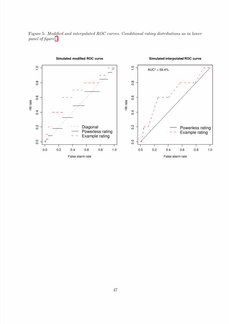
Of course, there is some overlap between examples 3.9 and 3.10. The samples in example 3.10could have been generated from rating distributions as described in example 3.9 (see lower panelof figure 3 for illustration). Then example 3.10 just would be a special case of example 3.9. Themore interesting case in example 3.10 therefore is the case where {x1, . . . , xnD}∩{y1, . . . , ynN } =

14

8/13/2019 Tasche_2009


∅. This will occur with probability 1 when the two sub-samples are generated from continuousscore distributions.

Some consequences of discontinuity:

• In the settings of examples 3.9 and 3.10 the CAP and ROC graphs as defined by (3.1b)and (3.1a) consist of finitely many points.

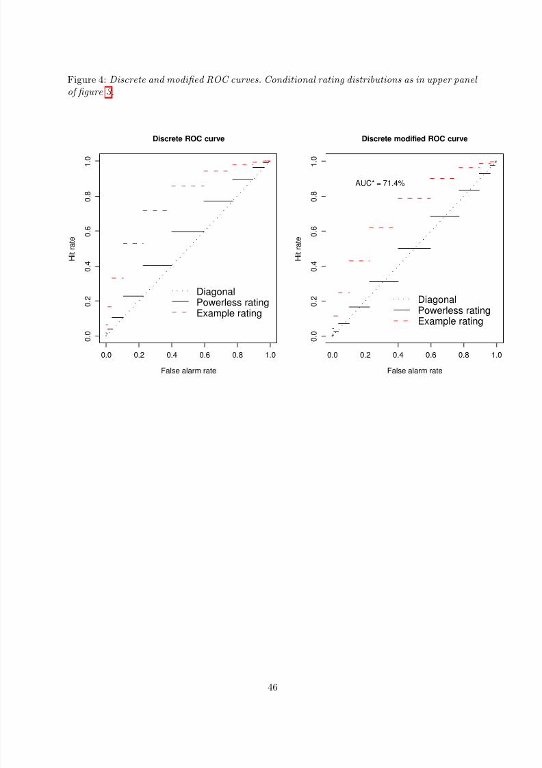
• CAP and ROC functions as defined by (3.5b) and (3.5a) are piecewise constant for ratinggrade variables R as in example 3.9 and empirical distribution functions as in example3.10. See left panel of figure 4 for illustration.

• Proposition 3.4 does not apply. In particular, the graphs of CAP and ROC functions asdefined by (3.5b) and (3.5a) for powerless score functions with discontinuities are notidentical with the diagonal line. See left panel of figure 4 for illustration.

• Let S be a random variable with a distribution that is concentrated on finitely many points

as in example 3.9 or 3.10. Let S be a random variable with the same distribution as S but independent of S . Then we have

P[S = S ] > 0. (3.21)

3.2.1 Observations on the general case

In this section, we first look at what happens with corollary 3.7 if no continuity assumptionobtains.

Proposition 3.11 (AUC and AR in the general case)Define AUC and AR by (3.10a) and (3.10b), respectively, with ROC and CAP as given in (3.5a)and (3.5b). Let S D and S N denote independent random variables with distribution functions F D(score distribution conditional on default) and F N (score distribution conditional on survival).Assume that S D is an independent copy of S D. Then

AUC = P[S D ≤ S N ],

AR = 2 P[S D ≤ S N ] − 1 + p

1 − p P[S D = S D].

Proof. The equation for AUC follows from application of Fubini’s theorem to the right-hand

side of (3.10a). Observe that in general

2 P[S D ≤ S D] = 1 + P[S D = S D] (3.22a)

and therefore

P[S D ≤ S D] − 1/2 = P[S D = S D]/2. (3.22b)

Inserting this last identity into (3.11) yields the equation for AR.

15

8/13/2019 Tasche_2009


Corollary 3.12 Define AUC and AR by (3.10a) and (3.10b), respectively, with ROC and CAP as given in (3.5a) and (3.5b). Let S D and S D denote independent random variables with dis-tribution function F D. In case of a powerless classification system (i.e. F D = F N ) we then have

AUC = 1/2 + P[S D = S D]/2,

AR = P[S D = S D]

1 − p .

(3.23)

In case of a perfect classification system (i.e. there is a score value s0 such that F D(s0) =1, F N (s0) = 0) we have

AUC = 1 (3.24a)

and, if p > 0,

AR = 1 + p

1 − p P[S D = S

D]. (3.24b)

When corollary 3.12 is compared to corollary 3.7, it becomes clear that definitions (3.5a) and(3.5b) are unsatisfactory when it comes to calculate AUC and AR for powerless or perfect scorefunctions with potential discontinuities. In particular, AUC and AR of powerless score functionsthen will not equal any longer 50% and 0, respectively. AR of a perfect score function can evenbe greater than 100% when calculated for a score function with discontinuities.

Definitions (3.5a) and (3.5b) of ROC and CAP curves, however, can be modified in a way suchthat proposition 3.6 and corollary 3.7 obtain without the assumption that the score function iscontinuous.

Definition 3.13 (Modified ROC and CAP functions)Denote by F N and F D the distribution functions of the survivor scores and the defaulter scores respectively. Let S D be a random variable with distribution function F D. The Modified ReceiverOperating Characteristic function ROC∗(u) then is defined by

ROC∗(u) = P

S D < F −1N (u)

+ P

S D = F −1N (u)

/2, u ∈ [0, 1]. (3.25a)

With F denoting the unconditional distribution function of the scores, the Modified CumulativeAccuracy Profile function CAP∗(u) is defined by

CAP∗(u) = PS D < F −1(u)+ PS D = F −1(u)/2, u∈

[0, 1]. (3.25b)

In general, we have

ROC∗(u) ≤ ROC(u) and CAP∗(u) ≤ CAP(u), u ∈ [0, 1].

Compare the two panels of figure 4 for illustration. If, however, the distribution function F Dof the defaulter scores is continuous, (3.25a) and (3.5a) are equivalent, and so are (3.25b) and(3.5b) because

ROC(u) = P

S D < F −1N (u)

+ P

S D = F −1N (u)

,

CAP(u) = PS D < F −1(u)+ PS D = F −1(u).(3.26)

16

8/13/2019 Tasche_2009


The following modified definitions of AUC and AR obviously coincide with the unmodified con-cepts of AUC and AR from definition 3.5 when the underlying score distributions are continuous.

Definition 3.14 (Modified area under the curve and modified accuracy ratio)For the function ROC∗ given by (3.25a) we define the modified area under the curve AUC∗ by

AUC∗ =

10

ROC∗(u) du. (3.27a)

For the function CAP∗ given by (3.25b) we define the modified accuracy ratio AR∗ by

AR∗ = 2

1 − p

10

CAP∗(u) du − 1/2

. (3.27b)

Clearly, we have AUC∗ ≤ AUC and AR∗ ≤ AR. The advantage of definition 3.14 compared todefinition 3.5 is that it gives us versions of proposition 3.6 and corollary 3.7 that obtain without

any continuity requirements on the score distributions.

Proposition 3.15 Define AUC∗ and AR∗ by (3.27a) and (3.27b), respectively, with ROC∗ and CAP∗ as given in (3.25a) and (3.25b). Let S D and S N denote independent random variables that have the distribution of the scores conditional on default and on survival respectively. Then we obtain

AUC∗ = P[S D < S N ] + P[S D = S N ]/2, (3.28a)

AR∗ = 2 P[S D < S N ] + P[S D = S N ] − 1 = P[S D < S N ] − P[S D > S N ]. (3.28b)

In particular, AR∗ = 2 AUC∗ − 1 holds.

Proof. By application of Fubini’s theorem, obvious from the definitions of AUC∗ and AR∗.

Note that (3.28a) by some authors (e.g. Newson, 2001, equation (12)) is used as definition of the area under the ROC curve.

Corollary 3.16 In case of a powerless classification system (i.e. F D = F N ) we have

AUC∗ = 1/2,

AR∗ = 0.(3.29)

In case of a perfect classification system (i.e. there is a score value s0 such that F D(s0) =1, F N (s0) = 0) we have

AUC∗ = 1 (3.30a)

and, if p > 0,

AR∗ = 1. (3.30b)

Corollary 3.16 gives a clear indication that for general score distributions definition 3.14 shouldbe preferred to definition 3.5. For the latter definition leads to the results from corollary 3.12that are counter-intuitive in case of discontinuous score distributions. In section 3.2.2, we willshow that in the settings of examples 3.9 and 3.10 definition 3.14 also can be interpreted ingraphical terms.

17

8/13/2019 Tasche_2009


3.2.2 Examples: Rating distributions and empirical score distributions

In this section, we look at examples 3.9 and 3.10 in more detail. Observe first that both examplescan be described in the same more general terms.

Assumption G: There is a finite number of states z1 < z2 < .. . < z such that

P[S D ∈ {z1, . . . , z}] = 1 = P[S N ∈ {z1, . . . , z}]. (3.31a)

Define for i = 1, . . . ,

P[S D = zi] = πi,

P[S N = zi] = ωi.(3.31b)

Convention:z0 = −∞. (3.31c)

To avoid redundancies in the notation we assume that

πi + ωi > 0 for i ≥ 1. (3.31d)

Choose = n and zi = i to see that (3.31a) (assumption G) is satisfied in the setting of example3.9. Then it is obvious how to determine the probabilities πi and ωi.

In case of example 3.10 choose to be the number of elements of the set (combined sample){x1, . . . , xnD , y1, . . . , ynN } and zi as the i-th element of the ordered list of the different elementsof the set. In this case we will have 1 ≤ ≤ nD + nN . The lower extreme case will occur whenboth the defaulter score sample and the survivor score sample are constant and have the same

value. This seems unlikely to happen in practice. The greater limit for will be assumed whenall the values in both the defaulter score and the survivor score samples are pairwise different.This will occur even with probability one if both conditional score distributions are continuous.

For the probabilities πi and ωi in (3.31b), in the setting of example 3.10 we obtain

πi = δ zi(x1, . . . , xnD) − δ zi−1(x1, . . . , xnD),

ωi = δ zi(y1, . . . , ynN ) − δ zi−1(y1, . . . , ynN ).(3.32)

ROC, ROC∗, AUC, and AUC∗. Under (3.31a) (assumption G), the ROC and ROC∗ func-tions according to (3.5a) and (3.25a) can be described more specifically as follows:

ROC(u) =

0, if 0 = u,i

j=1 π j, if i−1

j=1 ω j < u ≤i j=1 ω j

for 1 ≤ i ≤ .

(3.33a)

ROC∗(u) =

0, if 0 = u,

πi/2 +i−1

j=1 π j , if i−1

j=1 ω j < u ≤i j=1 ω j

for 1 ≤ i ≤ .

(3.33b)

18

8/13/2019 Tasche_2009


Remark 3.17 Observe that equations (3.33a) and (3.33b) can be become redundant to some extent in so far as the intervals on their right-hand sides may be empty. This will happen in particular in the context of example 3.10 whenever the samples x1, . . . , xnD and y1, . . . , ynN are disjoint. Let

y1 < . . . <

ykN be the ordered elements of the set {y1, . . . , ynN } of survivor scores.

Define y0 = −∞. More efficient versions of (3.33a) and (3.33b) then can be stated as

ROC(u) =

0, if 0 = u,

δ yk(x1, . . . , xnD), if δ yk−1(y1, . . . , ynN ) < u ≤ δ yk(y1, . . . , ynN )

for 1 ≤ k ≤ .

ROC∗(u) =

0, if 0 = u,

δ ∗yk

(x1, . . . , xnD), if δ yk−1(y1, . . . , ynN ) < u ≤ δ yk(y1, . . . , ynN )

for 1 ≤ k ≤ .

Under (3.31a) (assumption G) we obtain for the set gROC from definition 3.1

gROC =

00

,

ω1π1

,

ω1 + ω2π1 + π2

, . . . ,

−1 j=1 ω j−1 j=1 π j

,

11

. (3.34)

Under assumption (3.31d), the points in gROC will be pairwise different. Hence there won’t beany redundancy in the representation (3.34) of gROC.

As both the graphs of the ROC and the ROC∗ functions as specified by (3.33a) and (3.33b) canobviously be discontinuous at u = 0, u = ω1, . . ., u =

−1 j=1 ω j, in practice (see, e.g., Newson,

2001; Fawcett, 2004; Engelmann et al., 2003b) they are often replaced by the linearly interpolatedgraph through the points of the set gROC as given by (3.34) (in the order of the points as listed

there).

Proposition 3.18 Under (3.31a) (assumption G), the area in the Euclidean plane enclosed by the x-axis, the vertical line through x = 1 and the graph defined by linear interpolation of the ordered point set gROC as given by (3.34) equals AUC∗ as defined by (3.27a) and (3.33b).Moreover, AUC∗ can be calculated as

AUC∗ = 1/2

i=1

ωi πi +

i=2

ωi

i−1 j=1

π j. (3.35a)

Proof. Engelmann et al. (2003b, section III.1.2) showed that the area under the interpolatedROC curve equals AUC∗ as represented by (3.28a). Equation (3.35a) follows immediately from(3.28a) and (3.31b).

Still under (3.31a) (assumption G), it is easy to see that AUC from definition 3.5, i.e. the“continuous” version of the area under the curve, can be calculated as

AUC =

i=2

ωi

i j=1

π j ≥ AUC∗. (3.35b)

Observe that AUC = AUC∗ if and only if

i=1 ωi πi = P[S D = S N ] = 0.

19

8/13/2019 Tasche_2009


Remark 3.19 In the specific setting of example 3.10 , the representation of ROC∗(u) from re-mark 3.17 implies

AUC∗ = (nD nN )−1

nD

i=1nN

j=1δ ∗yj(xi). (3.36a)

The right-hand side of (3.36a) is up to the factor nD nN identical to the statistic of the Mann-Whitney test on whether a distribution is stochastically greater than another distribution (see,e.g., Engelmann et al., 2003b). By means of the representation of ROC(u) from remark 3.17 , it is not either hard to show that

A U C = (nD nN )−1

nDi=1

nN j=1

δ yj (xi). (3.36b)

Clearly, AUC∗ = AUC if and only if the samples x1, . . . , xnD and y1, . . . , ynN are disjoint.

CAP, CAP∗

, AR, and AR∗

. Recall from (2.2) that p stands for the unconditional probabilityof default5. Under (3.31a) (assumption G), (3.31b) therefore implies that P[S = zi] = p πi + (1− p) ωi. With this in mind, the following representations of CAP(u) and CAP∗(u) are obvious:

CAP(u) =

0, if 0 = u,i

j=1 π j, if i−1

j=1

p π j + (1 − p) ω j

< u ≤i

j=1

p π j + (1 − p) ω j

for 1 ≤ i ≤ .

(3.37a)

CAP∗(u) =

0, if 0 = u,

πi/2 +i−1

j=1 π j , if i−1

j=1

p π j + (1 − p) ω j

< u ≤i

j=1

p π j + (1 − p) ω j

for 1 ≤ i ≤ .

(3.37b)

Note that thanks to assumption (3.31d) the redundancy issue mentioned in remark 3.17 will notoccur for representations6 (3.37a) and (3.37b).

Under (3.31a) (assumption G) we obtain for the set gCAP from definition 3.1

gCAP =

00

,

p π1 + (1 − p) ω1

π1

, . . . ,

−1 j=1

p π j + (1 − p) ω j

−1 j=1 π j

,

11

. (3.38)

As the both the graphs of the CAP and the CAP∗ functions as specified by (3.37a) and (3.37b)are obviously discontinuous at u = 0, u = p π1 + (1

− p) ω1, . . ., u =

−1 j=1 p π j + (1

− p) ω j, in

practice (see, e.g., Engelmann et al., 2003b) they are often replaced by the linearly interpolatedgraph through the points of the set gCAP as given by (3.38) (in the order of the points as listedthere).

Proposition 3.20 Under (3.31a) (assumption G), the ratio of 1) the area in the Euclidean plane enclosed by the line x = y, the vertical line through x = 1 and the graph defined by linear

5In example 3.9, the value of p is a model parameter that can be chosen as it is convenient. In contrast, inexample 3.10 a natural (but not necessary) choice for the value of p is p = nD

nD+nN .

6For more efficient calculations of CAP(u) or CAP∗(u) in the setting of example 3.10 nonetheless the obser-vation might be useful that

i

j=1

p πj + (1− p) ωj

= δ zi(x1, . . . , xnD , y1, . . . , ynN ) if p is chosen as suggested in

footnote 5.

20

8/13/2019 Tasche_2009


interpolation of the ordered point set gCAP as given by (3.38) and 2) the area enclosed by the line x = y, the vertical line through x = 1 and the CAP ∗ curve of a perfect score function equals AR∗ as defined by (3.27b) and (3.37b). Moreover, AR∗ can be calculated as

AR∗ =

i=1

ωi πi + 2

i=2

ωi

i−1 j=1

π j − 1. (3.39a)

Proof. As in Engelmann et al. (2003b, section III.1.2) one can show that the area under the in-terpolated CAP curve equals P[S D < S ]+P[S D = S ]/2 where S D and S are independent randomvariables with the empirical distribution of the scores conditional on default and the uncondi-tional empirical score distribution, respectively. If S N denotes a further independent randomvariable, with the distribution of the scores conditional on survival, and S D is an independentcopy of S D, this observation implies that

Ratio of the areas 1) and 2) = P[S D < S ] + P[S D = S ]/2 − 1/2

1 − p/2 − 1/2

= 2

1 − p

p P[S D < S D] + (1 − p) P[S D < S N ]

+ P[S D = S D]/2 + (1 − p) P[S D = S N ]/2

= 2 P[S D < S N ] + P[S D = S N ] − 1.

By proposition 3.15, this implies the first part of the assertion. (3.39a) then is an immediateconsequence of (3.35a) and proposition 3.15 once again.

Still under (3.31a) (assumption G), by proposition 3.11 one can conclude that AR from definition3.5, i.e. the “continuous” version of the accuracy ratio, can be calculated as

A R = 2

i=2

ωi

i j=1

π j − 1 + p

1 − p

i=1

π2i > AR∗. (3.39b)

The “>” on the right-hand side of (3.39b) is implied by (3.31a) (i.e. at least one πi is positive).

Remark 3.21 In the specific setting of example 3.10, equation (3.39a) is equivalent to

AR∗ = 2

nD nN

nDi=1

nN j=1

δ ∗yj(xi) − 1. (3.40a)

If p = nDnD+nN

, by combining proposition 3.11 and (3.36b) one can also calculate AR for the setting of example 3.10 , i.e. a representation equivalent to (3.39b):

AR = 2

nD nN

nDi=1

nN j=1

δ yj(xi) − 1 + 1

nD nN

nDi=1

nD j=1

δ xj(xi) δ xi(x j). (3.40b)

Note that AR > AR∗ even if the samples x1, . . . , xnD and y1, . . . , ynN are disjoint. This follows from

nDi=1

nD j=1 δ xj(xi) δ xi(x j) ≥nD

i=1 1 = nD > 0.

21

8/13/2019 Tasche_2009


4 Discriminatory power: Numerical aspects

Engelmann et al. (2003a,b) compared for different sample sizes approximate normality-basedand bootstrap confidence intervals for AUC. As they worked with a huge dataset of defaulter

and non-defaulter scores, they treated the estimates on the whole dataset as “true” values – anassumption confirmed by tight confidence intervals. Engelmann et al. then sub-sampled fromthe dataset to study the impact of smaller sample sizes. Their conclusion – for scores both oncontinuous and discrete scales – was that even for defaulter samples of size ten the approximateand bootstrap intervals do not differ much and cover the “true” value.

After having presented some general considerations on the impact on bootstrap performanceby sample size in sub-section 4.1, in sections 4.2 and 4.3 we supplement the observations of Engelmann et al. in a simulation study7 where we sample from known analytical distributions.This way, we really know the true value of AUC and can determine whether or not the truevalue is covered by a confidence interval. Additionally, we study the impact of having an evensmaller sample size of five defaulters.

Note that by proposition 3.15 any conclusion on estimation uncertainty for AUC∗ also appliesto AR∗.

4.1 Bootstrap confidence intervals when the default sample size is small

Davison and Hinkley (1997, section 2.3) commented on the question of how large the samplesize should be in order to generate meaningful bootstrap samples. Davison and Hinkley observedthat if the size of the original sample is n the number of different bootstrap samples that canbe generated from this sample is no larger than

2n−1n

. Table 1 shows the value of this term for

the first eleven positive integers. When following the general recommendation by Davison andHinkley to generate at least 1000 bootstrap samples, according to table 1 then beginning withn = 7 it is possible not to have any identical (up to permutations) samples. For sample size sixand below the sample variation will be restricted for combinatorial reasons. This applies evenmore to samples on a discrete scale which in most cases include ties. One should therefore expectthat bootstrap intervals for AUC become less reliable when the size of the defaulter score sampleis six or less or when the sample includes ties. A simple simulation experiment further illustratesthis observation. For two samples of size n ∈ {1, . . . , 11} with n different elements and n − 1different elements respectively, we run8 100 bootstrap experiments each with 1000 iterations. Ineach bootstrap experiment we count how many of the generated samples are different.

Table 2 indeed clearly demonstrates that the factual sample size from bootstrapping is signifi-

cantly smaller than the nominal bootstrap sample size when the original sample has less thannine elements. The impact of small size of the original sample is even stronger when the originalsample includes at least one tie (two identical elements). Observe, however, that the impact of diminished factual sample size is partially mitigated by the fact that for combinatorial reasonsthe frequencies of duplicated bootstrap samples will have some variation.

7Like Engelmann et al. (2003a,b) we compare approximate normality-based and bootstrap confidence intervalsfor AUC. Newson (2006) describes how jackknife methods can be applied to estimate confidence intervals forSomers’ D (and hence in particular for AUC).

8All calculations for this paper were conducted with R version 2.6.2 (R Development Core Team, 2008).

22

8/13/2019 Tasche_2009


Bootstrap confidence intervals. In sections 4.2 and 4.3 we calculate basic bootstrap intervals generated by nonparametric bootstrap as described in section 2.4 of Davison and Hinkley (1997).Technically speaking, if the original estimate of a parameter (e.g. of AUC ∗) is t and we havea bootstrap sample t∗1 ≤ t∗2 ≤ . . . ≤ t∗n of estimates for the same parameter, then the basicbootstrap interval I at confidence level γ

∈(0, 1) is given by

I = [2 t − t∗n (1+γ )/2, 2 t − t∗n (1−γ )/2], (4.1)

where we assume that (n + 1) (1 + γ )/2 and (n + 1)(1 − γ )/2 are integers in the range from 1to n. Our standard choice of n and γ in sections 4.2 and 4.3 is n = 999 and γ = 95%, leading to(n + 1) (1 + γ )/2 = 975 and (n + 1) (1 − γ )/2 = 25.

Approximate confidence intervals for AUC∗ based on the central limit theorem.Additionally, in sections 4.2 and 4.3 we calculate approximate confidence intervals for AUCaccording to Engelmann et al. (2003b, equation (12)).

4.2 Simulation study: Continuous score distributions

We consider the normal distribution example from section 3.1.1 with the following choice of parameters:

µD = 6.8, σD = 1.96

µN = 8.5, σN = 2(4.2)

These parameters are chosen such as to match the first two moments of the binomial distributionslooked at in subsequent section 4.3. According to (3.14), under the normal assumption withparameters as in (4.2) then we have AUC = AUC∗ = 71.615%.

For defaulter score sample sizes nD ∈ {5, 10, 15, 20, 25, 30, 35, 40, 45, 50} and constant survivorscore sample size nN = 250, we conduct k = 100 times the following bootstrap experiment:

1) Simulate a sample of size nD of independent normally distributed defaulter scores and asample of size nN of independent normally distributed survivor scores, with parameters asspecified in (4.2).

2) Based on the samples from step 1) calculate estimates AUCkernel according to (3.18) and(3.19c) and AUCemp according to (3.36a) for AUC.

3) Based on the samples from step 1) and AUCemp calculate the normal 95% confidence

interval I normal (as described by Engelmann et al., 2003b, equation (12)).4) Generate for each of the two samples from step 1) r = 999 nonparametric bootstrap

samples, thus obtaining r = 999 pairs of bootstrap samples.

5) For each pair of bootstrap samples associated with bootstrap trial i = 1, . . . , r calculate

estimates AU C i according to (3.18) and (3.19c) as well as AU C i according to (3.36a) forAUC.

6) Calculate basic bootstrap 95% confidence intervals I kernel and I emp as described in (4.1)

based on the estimate AUCkernel and the sample AU C i

i=1,...,r

and the estimate AUCemp

and the sample AU C ii=1,...,r, respectively.

23

8/13/2019 Tasche_2009


7) Check whether or not

AUC ∈ I normal, AUC ∈ I kernel, AUC ∈ I emp,

50% ∈ I normal, 50% ∈ I kernel, 50% ∈ I emp.

To give an impression of the variation encountered with the different confidence interval method-ologies and the different sample sizes, table 3 (for defaulter sample sizes nD = 5, nD = 25, andnD = 45) shows the AUC estimates from the original samples and the related confidence intervalestimates for the first five experiments. Although it is clear from the tables that the estimatesare more stable and the confidence intervals are tighter for the larger defaulter score samples,it is nonetheless hard to conclude from these results which of the estimation methods is mostefficient.

Table 4 and figure 6 therefore provide information on how often the true AUC was covered by theconfidence intervals and how often 50% was an element of the confidence intervals. The check of the coverage of 50% is of interest because as long as 50% is included in a 95% confidence interval

for AUC, one cannot conclude that the score function or rating system under consideration hasgot any discriminatory power.

According to table 4 and figure 6 coverage of the true AUC is poor for defaulter sample sizenD ≤ 15 but becomes satisfactory for the larger defaulter sample sizes. At the same time, thevalues of coverage of 50% indicate poor power for defaulter sample sizes nD ≤ 20 and muchbetter power for defaulter sample size nD = 25 and larger.

For all defaulter sample sizes the coverage differences both for true AUC and for 50% are negli-gible in case of the “empirical” confidence intervals and the kernel estimation-based confidenceintervals. For the smaller defaulter sample sizes (nD ≤ 15), coverage of true AUC by the normalconfidence interval is clearly better than by the “empirical” confidence intervals and the kernelestimation-based confidence intervals but still less than the nominal level of 95%. The bettercoverage of true AUC by the normal confidence intervals, however, comes at the price of a muchhigher coverage of 50% for defaulter samples sizes nD ≤ 20 (type II error). For defaulter samplesizes nD ≥ 25 differences in performance of the three approaches to confidence intervals seem tovanish.

Remark 4.1 With a view on (3.36a), it follows from the duality of tests and confidence intervals (see, e.g., Casella and Berger , 2002, theorem 9.2.2) that the check of whether 50% is covered by the AUC 95% confidence interval is equivalent to conducting a Mann-Whitney test of whether the defaulter score distribution and the survivor score distribution are equal (null hypothesis). The

exact distribution of the Mann-Whitney test statistic can be calculated with standard statistical software packages. Hence the 95% confidence interval coverage rates of 50% reported in table 4can be double-checked against type II error rates from application of the two-sided Mann-Whitney test at 5% type I error level.

The type II error rates mentioned in remark 4.1 are displayed in the second to last column of table 4. For the sake of completeness, in the last column of table 4 type II error rates fromapplication of the two-sided Kolmogorov-Smirnov test are presented, too. Comparison of theMann-Whitney type II error and the coverage of 50% by the AUC confidence intervals clearlyindicates that for defaulter sample size nD ≤ 20 the bootstrap confidence intervals are toonarrow. With a view on table 2 this observation does not come as a surprise for very small

24

8/13/2019 Tasche_2009


defaulter sample sizes but is slighly astonishing for a defaulter sample size like nD = 15. Theconfidence intervals based on asymptotic normality, however, seem to perform quite well forsample size nD ≥ 10. Comparing the last column of table 4 to the second-last column moreovershows that the Mann-Whitney test is clearly more powerful for smaller defaulter sample sizesthan the Kolmogorov-Smirnov test.

In summary, the simulation results suggest that in the continuous setting of this section fordefaulter sample size nD ≥ 20 the performance differences between the three approaches toAUC confidence intervals considered are negligible. For defaulter sample size nD < 20, however,with a view on the coverage of the true AUC parameter it seems clearly preferable to deploy theconfidence interval approach based on asymptotic normality (as described, e.g., by Engelmannet al., 2003a,b) because its coverage rates come closest to the nominal confidence level (butare still smaller). For very small defaulter sample size nD ≤ 10, poorer coverage of the trueAUC parameter may come together with a high type II error (high coverage of 50%, indicatingmisleadingly that the score function is powerless).

On the basis of a more intensive simulation study that includes observations on coverage rates,thus we can re-affirm and at the same time refine the conclusion by Engelmann et al. (2003a,b)that confidence intervals for AUC (and AR) based on asymptotic normality work reasonably wellfor sample data on a continuous scale, even for small defaulter sample size like nD = 10 but notnecessarily for a very small defaulter sample size like nD = 5. Moreover, for defaulter sample sizesnD < 20 the asymptotic normality confidence interval estimator out-performs bootstrap-basedestimators.

4.3 Simulation study: Discrete score distributions

We consider the binomial distribution example for 17 rating grades from figure 3 with probability

parameter pD = 0.4 for the defaulter rating distribution and probability parameter pN = 0.5for the survivor rating distribution. As a consequence, the first two moments of the defaulterrating distribution match the first two moments of the defaulter score distribution from section4.2 and the first two moments of the survivor rating distribution match the first two moments of the survivor score distribution from section 4.2. Moreover, also the discriminatory power of thefictitious rating system considered in this section is almost equal to the discriminatory power of the score function from section 4.2 (AUC∗ 71.413% according to (3.35a) vs. AUC 71.615%).

To assess the impact of the discreteness of the model, we conduct the same simulation exerciseas in section 4.2 but replace step 1) by step 1∗) which reads

1∗) Simulate a sample of size nD of independent binomially distributed defaulter ratings and asample of size nN of independent binomially distributed survivor ratings, with probabilityparameters pD = 0.4 and pN = 0.5 respectively.

As in section 4.2, to give an impression of the variation encountered with the different confidenceinterval methodologies and the different sample sizes, table 5 (for defaulter sample sizes nD = 5,nD = 25, and nD = 45) shows the AUC estimates from the original samples and the relatedconfidence interval estimates for the first five experiments. Although it is clear from the tablesthat the estimates are more stable and the confidence intervals are tighter for the larger defaulterscore samples, it is nonetheless hard to conclude from these results which of the estimationmethods is most efficient. Interesting is also the result from experiment number 5 for sample

25

8/13/2019 Tasche_2009


size nD = 5 in table 5 which with lower confidence bounds of 90.0% and more looks very muchlike an outlier due to a defaulter sample concentrated at the bad end of the rating scale.

Table 6 and figure 7 provide information on how often the true AUC was covered by the con-fidence intervals and how often 50% was an element of the confidence intervals. In contrast to

table 4 and figure 6, table 6 and figure 7 do not give a very clear picture of the performanceof the three AUC estimation approaches on the rating data. While coverage of 50% (type IIerror) is high for defaulter sample sizes smaller than nD = 30, coverage of 50% reaches verysmall values as in the continuous case of section 4.2 for larger defaulter sample sizes. Presumablydue to the relatively small number of 100 bootstrap experiments – which already requires somehours of computation time –, according to figure 7 there is some variation and not really a cleartrend in the level of coverage of the true AUC parameter. Even for a relatively high defaultersample size of nD = 40 there is sort of a collapse of coverage of true AUC with percentages of 90% or lower. For defaulter sample size of nD = 45 or more there might be some stabilisationat a satisfactory level.

As in the continuous case, for all defaulter sample sizes the coverage differences both for trueAUC and for 50% are negligible in case of the “empirical” confidence intervals and the kernelestimation-based confidence intervals. For the smaller defaulter sample sizes (nD ≤ 20), coverageof true AUC by the normal confidence interval is clearly better than by the “empirical” confidenceintervals and the kernel estimation-based confidence intervals but still less than the nominal levelof 95%. The better coverage of true AUC by the normal confidence intervals, however, comesat the price of a much higher coverage of 50% for defaulter samples sizes nD ≤ 15 (type IIerror). For defaulter sample sizes nD ≥ 25 differences in performance of the three approaches toconfidence intervals seem to vanish.

Remark 4.2 Remark 4.1 essentially also applies to the setting of this section. But take into

account that in the presence of ties in the sample the equivalence between AUC∗

as defined by (3.27a) and the Mann-Whitney statistic only holds when ranks for equal elements of the ordered total sample are assigned as mid-ranks. With this in mind we can double-check the 95% confidence coverage rates of 50% reported in table 6 against type II error rates from application of the two-sided Mann-Whitney test at 5% type I error level in the same manner as we have done for remark 4.1.

The type II error rates9 mentioned in remark 4.2 are reported in the second to last column of table6. We have presented type II error rates from application of the two-sided Kolmogorov-Smirnovtest in the last column of table 4. Due to the massive presence of ties in the discrete-case samples,however, application of the Kolmogorov-Smirnov test does not seem appropriate in this section.

Instead, we report type II error rates from application of the two-sided exact Fisher test 10 (see,e.g., Weisstein, 2009) in the last column of table 6.

Again, comparison of the Mann-Whitney type II error and the coverage of 50% by the AUCconfidence intervals clearly indicates that for defaulter sample size nD ≤ 20 the bootstrapconfidence intervals are too narrow. With another view on table 2 this is even less a surprisethan in the continuous case. The confidence intervals based on asymptotic normality, however,

9Exact p-values for the Mann-Whitney test on samples with ties were calculated with the function wilcox test

from the R-software package coin .10The p-values of Fisher’s exact test have been calculated with the function fisher.test (R-software package

stats ) in simulation mode due to too high memory and time requirements of the exact mode.

26

8/13/2019 Tasche_2009


8/13/2019 Tasche_2009


when following a parametric approach to PD curve estimation. See Pluto and Tasche (2005) fora non-parametric approach that might be a viable alternative in particular when little defaultobservation is available.

5.1 Derivatives of CAP and ROC curves

It is a well known fact that there is a close link between ROC and CAP curves on the onehand and conditional probabilities of default on the other hand. Technically speaking, the linkis based on the following easy-to-prove (when making using of theorem 3.2) observation.

Proposition 5.1 Let F D and F N be distribution functions on an open interval I ⊂ R. Assume that F D has a density f D which is continuous on I and that F N has a positive density f N that is continuous on I . Let 0 < p < 1 be a fixed probability and define the mixed distribution F by (2.4). Write f for the density of F . Define ROC(u) and CAP(u), u ∈ (0, 1) by (3.5a) and (3.5b), respectively. Then both ROC and CAP are continuously differentiable for u

∈(0, 1) with

derivatives

ROC(u) = f D

F −1N (u)

f N

F −1N (u) , (5.1a)

CAP(u) = f D

F −1(u)

p f D

F −1(u)

+ (1 − p) f N

F −1(u)

= f D

F −1(u)

f

F −1(u) . (5.1b)

Proposition 5.1 is of high interest in the context of individual default risk analysis because – in

the notation of sections 2.2 and 3 – the probability of default conditional on a score value s isgiven by (2.6b). Proposition 5.1 then immediately implies

P[D | S = s] = p ROC

F N (s)

p ROC

F N (s)

+ 1 − p

(5.2a)

= p CAP p F D(s) + (1 − p) F N (s)

= p CAP

F (s)

. (5.2b)

Note that by (5.2b), the derivative of a differentiable CAP curve for a borrower populationwith unconditional probability of default p > 0 is necessarily bounded from above by 1/p. Thefollowing theorem shows on the one hand that this condition is not only a necessary but alsoa sufficient condition for a distribution function on the unit interval to be a CAP curve. Onthe other hand, the theorem shows that a CAP curve relates not only to one combination of conditional and unconditional score distributions but provides a link between conditional andunconditional score distributions which applies to an infinite number of such combinations.

Theorem 5.2 Let p ∈ (0, 1) be a fixed probability. Let f D ≥ 0 be a density on R such that the set I = {f D > 0} is an open interval and f D is continuous in I . Denote by F D(s) =

s−∞ f D(v) dv

the distribution function associated with f D. Then the following two statements are equivalent:

(i) The function u → C (u), u ∈ (0, 1) is continuously differentiable in u with limu→0

C (u) = 0,

limu→1

C (u) = 1, and 0 < C (u) ≤ 1/p, u ∈ (0, 1).

28

8/13/2019 Tasche_2009


(ii) There is a density f N ≥ 0 such that {f N > 0} = I , f N is continuous in I and

C (u) = F D

F −1(u)

, u ∈ (0, 1), (5.3)

where F (s) = p F D(s) + (1 − p) s−∞ f N (v) dv.

Proof.

(i) ⇒ (ii): By assumption, C maps (0, 1) onto (0, 1) and the inverse C −1 of C exists. DefineF (s) = C −1

F D(s)

. Then F is a distribution function with lim

s→inf I F (s) = 0, lim

s→sup I F (s) = 1

and density

f (s) = F (s) = f D(s)

C

F (s) , s ∈ I. (5.4)

Observe that f (s) is positive and continuous in I . Hence the inverse F −1 of F exists. Let

F N (s) =

F (s)

− p F D(s)

1 − p s ∈R

, and

f N (s) = f D(s) 1/C

F (s)− p

1 − p , s ∈ I. (5.5)

By (5.4), then f N is the continuous derivative of F N and is positive in I by assumption on C

and f D. This implies that F N is a distribution function with lims→inf I

F N (s) = 0, lims→sup I

F N (s) = 1

and density f N . By construction of F and F N , the functions C , F D, and F satisfy (5.3).

(ii) ⇒ (i): By construction, F D(s) and F (s) are distribution functions which converge to 0 fors → inf I and to 1 for s → sup I . This implies the limit statements for C . Equation (5.3) impliesthat C is continuously differentiable with derivative

0 < C (u) = f DF −1(u)

p f D

F −1(u)

+ (1 − p) f N

F −1(u) ≤ 1/p.

For the sake of completeness, we provide without proof the result corresponding to theorem5.2 for ROC curves. In contrast to the case of CAP curves, essentially every continuously dif-ferentiable and strictly increasing distribution function on the unit interval is the ROC curvefor an infinite number of combinations of score distributions conditional of default and survivalrespectively.

Proposition 5.3 Let f D

≥ 0 be a density on R such that the set I =

{f D > 0

} is an open

interval and f D is continuous in I . Denote by F D(s) = s−∞ f D(v) dv the distribution function associated with f D. Then the following two statements are equivalent:

(i) The function u → R(u), u ∈ (0, 1) is continuously differentiable in u with limu→0

R(u) = 0,

limu→1

R(u) = 1, and 0 < R(u), u ∈ (0, 1).

(ii) There is a density f N ≥ 0 such that {f N > 0} = I , f N is continuous in I and

R(u) = F D

F −1N (u)

, u ∈ (0, 1), (5.6)

where F N (s) = s−∞ f N (v) dv.

29

8/13/2019 Tasche_2009


The basic idea both with theorem 5.2 and proposition 5.3 is that if in the functional equationf (x) = g(h−1(x)) two of the three functions f , g and h are given then the third can be calculatedby solving the equation for it. In the cases of ROC and CAP curves, matters can get morecomplicated because the involved functions are not necessarily invertible. This would entail sometechnicalities when trying to solve f (x) = g(h−1(x)) for g or h. However, to relate conditionalprobabilities of default to ROC and CAP functions via (5.2a) and (5.2b) we need the existenceof densities. This introduces some degree of smoothness as can be seen from theorem 5.2 andproposition 5.3. Both the theorem and the proposition could also be stated with fixed distributionF N of the survivor scores. However, the survivor score distribution appears in the CAP functiononly as a mixture with the defaulter score distribution. Therefore, stating theorem 5.2 with givensurvivor score distribution would no longer be straight-forward and the proof would involve theimplicit function theorem. As the additional insight by such a version of theorem 5.2 would belimited, in this paper the formulation of the theorem as provided above has been preferred.

5.2 Van der Burgt’s approach and alternatives

The one-parameter curve proposed by van der Burgt (2008) for estimating CAP functions is

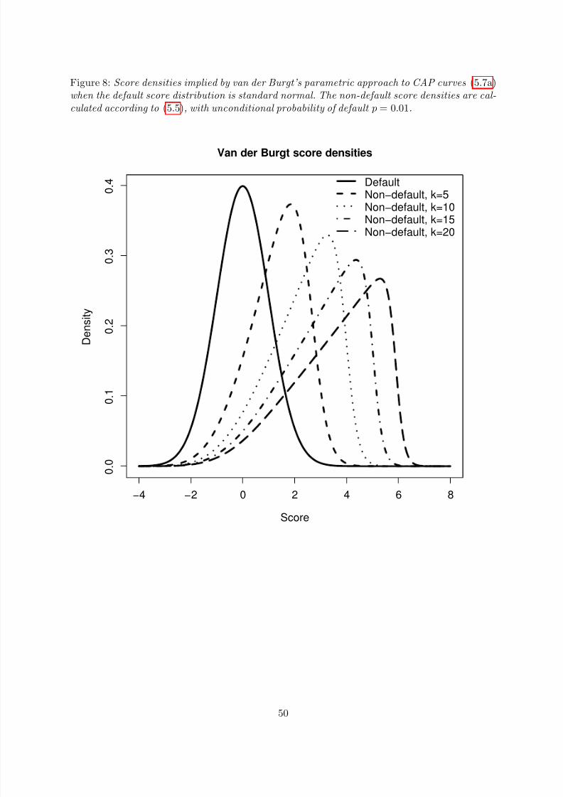
C κ(u) = 1 − e−κu

1 − e−κ , u ∈ [0, 1], (5.7a)

where κ ∈ R is the fitting parameter. The function C κ is obviously a distribution function on[0, 1]. Moreover, for positive κ the graph of C κ is concave as one might expect from the CAPcurve of a score function that assigns low scores to bad borrowers and high scores to goodborrowers. For κ → 0 the graph of C κ converges toward the diagonal line, i.e. the graph of apowerless score function. The derivative of C κ and ARκ associated with C κ according to (3.10b)

are easily computed as

C κ(u) = κ e−κu

1 − e−κ, (5.7b)

ARκ = 2

1 − p

1

1 − e−κ − 1

κ − 1/2

. (5.7c)

In (5.7c) the parameter p > 0 denotes the unconditional probability of default of the estimationsample in the sense of section 2.1. Observe from (5.7b) that for κ > 0

C κ(1) = κ

1 − e−κ e−κ ≤ C κ(u) ≤ κ

1 − e−κ = C κ(0), u ∈ [0, 1]. (5.8a)

Theorem 5.2 hence implies

κ < κ

1 − e−κ ≤ 1

p. (5.8b)

Given a CAP curve CAP(u) to be approximated, in the setting of a continuous score functiona natural approach to finding the best fit κ would be a least squares procedure as the following

κ = arg minκ>0

10

CAP(u) − C κ(u)

2du

= arg minκ>0

E

F D(S ) − C κ(F (S ))2

.

(5.9a)

30

8/13/2019 Tasche_2009


In practice, the integration in (5.9a) would have to be replaced by a sample mean. Alternatively,van der Burgt (2008) suggested inferring κ by means of (5.7c) from an estimated11 AR (orvia proposition 3.6 from an estimated AUC). Assuming that an estimate of the unconditionalprobability p is available, probabilities of default conditional on realised score values then canbe estimated via (5.2b):

P[D | S = s] = p κ e−κF (s)

1 − e−κ . (5.9b)

Van der Burgt (2008), however, applied the methodology to a discrete setting as described inexample 3.9 (rating system with n grades). In the notation of example 3.9 van der Burgt’sapproach to finding the best fit parameter κ can be described as

κ = arg minκ>0

n j=1

P[RD ≤ j] − C κ(P[R ≤ j])

2= arg min

κ>0E

F D(R) − C κ(F (R))

2

P[R = r] r=R .

(5.10a)

Van der Burgt’s approach hence can be regarded as sort of an unweighted regression in whichthe same weights are given to rating grades with very few observations and grades with quitea lot of observations. For calculating the estimates of the conditional probabilities of defaultvan der Burgt (2008) does not deploy equation (5.9b) but a modification that substitutes theunconditional score distribution function F by the mean of its right and left continuous versions(F + F ( · − 0))/2:

P[D | R = j ] = p κ exp

−κ (P[R < j] + P[R ≤ j])/2

1 − e−κ . (5.10b)

In his paper, van der Burgt (2008) does not spend much time with explaining the why and how

of his approach. It is tempting to guess that the approach was more driven by the results thanby theoretical considerations. We observe that it is not obvious how to deploy van der Burgt’sregression approach (5.10a) for a sample of scores from a score function with continuous scale.Therefore, for our example calculations in section 5.3 we will make use of (5.9a) and (5.9b) forthe continuous setting and of (5.10a) and (5.10b) for the discrete setting of example 3.9.

In general, when choosing C κ for fitting a CAP curve, one should be aware that as a consequenceof theorem 5.2 this choice implies some structural links between the score distribution of thedefaulters and the score distribution of the survivors. This is illustrated in figure 8 which showsfor unconditional probability of default p = 0.01 and different values of κ the survivor scoredensities that are implied by theorem 5.2 when the defaulter score density is assumed to be

standard normal. Clearly, for large κ and, by (5.7c), high discriminatory power the impliedsurvivor score distributions are not normal as they are not symmetric.

This observation on the one hand might be considered not very appealing. On the other hand,it suggests an alternative approach along the lines of section 3.1.1 which provides in (3.14) atwo-parametric representation of the ROC function for the case of normally distributed defaulterand survivor score distributions.

As mentioned in section 3.1.1, no closed form is available for the CAP function in case of normallydistributed defaulter and survivor score distributions. This is one reason why we consider in the

11This requires that there is an estimate of p. Van der Burgt assumes p ≈ 0 for the purpose of estimating κ butthen, in a further step, makes use of the fact that p is positive.

31

8/13/2019 Tasche_2009


following how to approximate general ROC curves (not CAP curves) by the ROC function of the normal family as described in section 3.1.1. Another reason is that, in general, fitting ROCcurves is conceptually sounder than fitting CAP curves because this way one can better separatethe estimation of an unconditional probability of default from the estimation of parameters of the fitting function.

By substituting in (3.14) the parameter b > 0 for σN /σD and the parameter a ∈ R for µN −µDσD,

we obtain a two-parametric family of ROC functions:

Ra,b(u) = Φ

a + b Φ−1(u)

, u ∈ (0, 1). (5.11a)

From this, it follows readily that

Ra,b(u) = b

ϕ

a + b Φ−1(u)

ϕ

Φ−1(u) , (5.11b)

ARa,b = 2 Φ

a√ b2 + 1

− 1. (5.11c)

Clearly, a two-parameter family of functions will give better fits than a one-parameter family of functions as the one-parameter family proposed by van der Burgt (2008). In order to have a faircomparison, therefore, in the following we will focus on the one-parameter sub-family of (5.11a)specified by fixing b at b = 1. We simplify notation by writing Ra for Ra,1. From section 3.1.1it follows that the one-parameter family of ROC functions Ra includes, in particular, the ROCcurves for normally distributed defaulter and survivor score functions when their variances areequal. Equations (5.11b) and (5.11c) are simplified significantly for Ra:

Ra(u) = e−aΦ

−1(u)−a2/2, (5.12a)

ARa = 2 Φa/√

2− 1. (5.12b)

When the unconditional probability of default p is known, (5.12a) via (5.2a) implies the followingrepresentation of the probability of default conditional on a realised score value:

P[D | S = s] = 1

1 + 1− p p exp

a Φ−1(F N (s)) + a2/2 . (5.13a)

Clearly, (5.13a) can be rewritten as

P[D | S = s] = 1

1 + exp

α + β Φ−1(F N (s)) (5.13b)

with

α = log1 − p

p

+ a2/2, β = a.

Thus, the conditional PDs derived from the one-parameter ROC approximation approach (5.11a)with b = 1 are the conditional PDs of a logit regression where the default indicator is regressed onthe explanatory variable Φ−1(F N (S )). In the special case where the score distribution conditionalon survival is normal (i.e. F N (s) = Φ

(s−µ)/σ

for some suitable constants µ and σ), the right-

hand side of equation (5.13b) coincides with the conditional PDs of the common logit approach:

P[D | S = s] = 1

1 + expα + β s. (5.14)

32

8/13/2019 Tasche_2009


Thus (5.13b) can be considered a robust logit approach that replaces regression on the originalscore S by regression on the transformed score Φ−1(F N (S )) to account for the fact that thescore distribution might not be normal. As such, the suggestion by van der Burgt (2008) leadsto a potentially quite useful modification of logit regression in the univariate case.

On an estimation sample in the sense of section 2.1.1, parameters for logit-type raw conditionalPDs as specified in equations (5.13b) and (5.14) can be estimated by maximum likelihood (MLE)procedures (see, e.g., Cramer, 2003, chapter 3). In the case of (5.13b), MLE will only work if 0 < F N (xi) < 1 and 0 < F N (y j) < 1 for all scores xi (defaulters) and y j (survivors) in theestimation sample. This will not be the case if F N is estimated as the empirical distributionfunction of the survivor sample y j. To work around this issue, the empirical distribution canbe modified (as described in section 5.3). Another approach could be non-linear least squaresestimation:

(

α,

β ) = arg min

α,β∈RE

1D − 1 + exp

α + β Φ−1(F N (S ))−12

, (5.15)

where 1D = 1 for defaulted borrowers and 1D = 0 otherwise.

Van der Burgt (2008, equation (5)) suggested inferring the value of parameter κ specifying hisCAP curve approximation (5.7a) from an estimate of AUC. This idea can be used to deriveanother approach to the estimation of the parameters in (5.13b) or (5.14). To infer the values of two parameters, two equations are needed. A natural choice for the first equation is to equate atarget value q for the unconditional PD and the mean of the conditional PDs:

q = E

P[D | S ]

. (5.16a)

This equation can in general be used for the calibration of conditional PDs, see appendix Afor details. A good choice for the second equation seems equating a target value A for the area

under the curve AUC∗ and a representation of AUC∗ in terms of the conditional PDs:

A =E

E

P[D | S ] 1{S<s}

s=S +P[S = s]

{s=S }

P[D | S ]/2

1 − P[D | S ]

E

P[D | S ]

1 − E

P[D | S ] (5.16b)

This representation of AUC∗ follows from proposition 3.15. Combining equations (5.16a) and(5.16b) for the inference of parameters can be regarded as a quasi moment matching approach.It is “quasi” moment matching because AUC∗ is not a proper moment of the conditional PDs.The most natural alternative, the variance of the conditional PDs, however, depends on theproportion of defaulters in the borrower population. As this proportion clearly varies over timeit would be difficult to determine an appropriate target variance of the conditional PDs. Incontrast, AUC∗ by its definition does not depend on the proportion of defaulters in the borrowerpopulation. It is therefore plausible to assume that discriminatory power displays less variationover time such that its value can be inferred from a historical estimation sample and still appliesto the current portfolio. The following example illustrates how the quasi moment matchingapproach works when the logit shape (5.14) is supposed to apply to the conditional PDs.

Example 5.4 (Quasi moment matching for PD curve calibration)Let s1 ≤ s2 ≤ . . . ≤ sn be a sorted calibration sample of credit scores in the sense of section 2.1.2 (possibly the scores of the current portfolio). Assume that the PDs conditional on the score

33

8/13/2019 Tasche_2009


realisations can be described by (5.14). The sample versions of equations (5.16a) and (5.16b)then read:

q = 1

n

n

i=11

1 + expα + β si,

A =

ni=1exp(α+β si)1+exp(α+β si)

12 (1+exp(α+β si))

+i−1

j=11

1+exp(α+β sj)

ni=1

11+exp(α+β si)

ni=1exp(α+β si)1+exp(α+β si)

.

(5.17)

Here q is the target unconditional PD which could be estimated for instance by econometric methods (see, e.g., Engelmann and Porath , 2003, section III). The variable A stands for the target discriminatory power, expressed as area under the curve AUC∗ which can be estimated

from an estimation sample in the sense of section 2.1.1 by means of (3.36a).Solving the equation system (5.17) for the parameters α and β then gives the quasi momentmatching coefficients for the logit approach to conditional PDs.

5.3 Performance comparison

To illustrate the operation of van der Burgt’s approach and the three logit approaches introducedin section 5.2 and to compare their performance, we get back to the example from section 4.2for the continuous score distribution case and to the example from section 4.3 for the case of a discrete rating distribution. The examples, together with some modifications, will show thatnone of the four approaches is uniformly superior to the others. To see how the estimationmethods work we conduct simulation experiments with five different scenarios.

The following scenarios are considered:

1) Rating systems with discrete scales:

• Case 1: 17 grades, binomial distribution with probability parameter 0.4 for the de-faulters’ rating distribution, binomial distribution with probability parameter 0.5 forthe survivors’ rating distribution (as in section 4.3).

• Case 2: 7 grades, binomial distribution with probability parameter 0.3 for the de-faulters’ rating distribution, binomial distribution with probability parameter 0.5 forthe survivors’ rating distribution.

2) Score functions with continuous scales:

• Case 3: Normal distribution with mean 6.8 and standard deviation 1.96 for the de-faulters’ score distribution, normal distribution with mean 8.5 and standard deviation2 for the survivors’ score distribution (as in section 4.2). Means and standard devia-tions are chosen such as to match those from the above discrete case 1.

• Case 4: Normal distribution with mean 2.1 and standard deviation 1.12 for the de-faulters’ score distribution, normal distribution with mean 3.5 and standard deviation1.22 for the survivors’ score distribution. Means and standard deviations are chosensuch as to match those from the above discrete case 2.

• Case 5: Normal distribution with mean 0.0 and standard deviation 1.25 for the de-faulters’ score distribution, normal distribution with mean 1.0 and standard deviation

34

8/13/2019 Tasche_2009


1.0 for the survivors’ score distribution. Means and standard deviations here are cho-sen such as to have a larger difference in standard deviations than in cases 3 and 4and to have the standard deviation for the defaulters’ score distribution exceedingthe standard deviation for the survivors’ score distribution.

In cases 1 and 2, when the value of the unconditional PD is known, the true conditional PDsper rating grade can be calculated according to (2.6a). In cases 3, 4, and 5 the true conditionalPDs per score value can be calculated according to (2.6b).

For each scenario the following simulation experiment with 1000 iterations is conducted:

1) Generate an estimation sample: Rating grades / scores of 25 (results in table 7) and 50(results in table 8) defaulters and rating grades / scores of 250 survivors.

2) Based on the estimation sample, estimates are calculated for

• discriminatory power measured by AUC∗

according to (3.36a),• parameters12 p and κ and distribution function13 F for the raw conditional PDs

suggested by van der Burgt (2008), where the PDs are calculated according to (5.9b)in the continuous cases 3, 4, and 5, and according to (5.10b) in the discrete cases 1and 2,

• parameters α and β and distribution function14 F N for the raw conditional PDsaccording to the robust logit approach (5.13b),

• parameters15 α and β for the raw conditional PDs according to the logit approach(5.14).

3) Generate then a calibration sample: Rating grades / scores of 300 borrowers with unknown

future solvency states. For each of the borrowers first a default / survival simulation withPD = 2.5% is conducted. According to the result then a rating grade / score is drawnfrom the corresponding rating / score distribution. The simulated solvency state is notrecorded.

4) Based on the calibration sample, the raw PDs from step 2) are calibrated to an uncondi-tional PD16 of 2.5%, as described in proposition A.1 from appendix A.

5) Based on the calibration sample, parameters α and β for PDs according to the quasimoment matching approach are inferred from an unconditional PD 2.5% and the AUC ∗

estimate from step 2), as described in example 5.17.

12Here p is actually a constant: p = 25/(25 + 250) = 1/11 and p = 50/(25 + 250) = 1/6 respectively.13In the continuous cases 3, 4, and 5, an estimate of F is calculated according to (2.4). F D and F N in (2.4) are

calculated from normal kernel density estimates with bias-correction as described in section 3.1.2. In the discretecases 1 and 2 the standard empirical distribution function is deployed for estimating F .

14In the continuous cases 3, 4, and 5, F N is calculated from a normal kernel density estimate with bias-correctionas described in section 3.1.2. In the discrete cases 1 and 2, F N is estimated as the mean of the right-continuousand the left-continuous versions of the empirical distribution function. Additionally, to avoid numerical issueswhen deploying maximum likelihood estimation, whenever the result would be zero it is replaced by half of theminimum positive value of the modified empirical distribution function.

15α and β are estimated by the standard logit MLE procedure (see, e.g., Cramer, 2003, chapter 3).16Hence, we implicitly assume that we have estimated exactly the true unconditional PD of 2.5%. Of course,

in practice this would be unlikely. For the purpose of comparing the performance of different estimators thisassumption is nonetheless useful.

35

8/13/2019 Tasche_2009


6) Based on the calibration sample, for each rating grade / score the differences betweentrue conditional PD and the PD estimates according to the four different approaches arecalculated.

7) Based on the four samples of PD differences, the standard error SE is calculated for each

of the four approaches according to the generic formula

SE =

1

n

ni=1

P[D | S = si] − P[D | S = si]

2, (5.18)

where s1, . . . , sn is the calibration sample, P[D | S = si] is the true conditional PD, and P[D | S = si] is the estimated conditional PD.

Actually, running the simulation as described in steps 1) to 7) only once would provide interestinginsights but would not help too much when it comes to a comparison of the performances of the different estimators. For illustration, have a look at figure 9 which displays the results (true

conditional PDs and estimated conditional PDs) of one simulation run of case 1 (17 rating gradesscenario). All four estimates seem to fit well the true conditional PDs for rating grades 5 to 17.For rating grades 1 to 4 the fit seems much worse. The van der Burgt and the robust logitestimators even assign constant conditional PD estimates to rating grades 1 to 3.

Note, however, that in this simulation run there were no observations of rating grades 1 to 3and 16 and 17. In so far, on the one hand, it is questionable whether there should be at all anyconditional PD estimates for grades 1 to 3 and 16 and 17. On the other hand, it is not surprisingthat also for the logit and quasi moment matching estimators the fit at grades 1 to 3 and 16 and17 is rather poor. Given the sizes of 300 or less of the estimation and calibration samples thatare simulated, full coverage of the rating scale by realised rating grades can only be expectedfor a rating scale with a significantly lower number of grades. In the following, therefore, welook also at the scenario case 2 – a rating system with 7 grades only. The probability to observeunoccupied rating grades when the sample size is about 250 is quite low under scenario case 2.

According to the single simulation run underlying figure 9 there might not be any dramaticdifferences of the performances of the different estimators. More detailed information can beobtained from running a number of simulations. Tables 7 and 8 (for defaulter scores samplesizes 25 and 50 respectively in the estimation sample) show quantiles of the distributions of thestandard errors according to (5.18) that were observed in 1000 iterations of the experiment.

Observations from tables 7 and 8:

(i) When comparing the quantiles of the standard error distributions as displayed in table 8to the results from table 7, it appears that the reductions in the low quantiles are moder-ate while the reductions in the higher quantiles are significantly larger. This observationindicates that the higher number of defaulter scores in the estimation sample mainly hasan impact on the variance of the standard error distributions. Note that the distributionalassumptions in cases 1 to 5 have been chosen deliberately such that exact matches by oneof the estimation approaches are not possible. Hence the standard error rates do not con-verge to zero for larger defaulter score samples. Rather the variances of their distributionswill be diminished.

(ii) For cases 1 to 3 the logit estimator is best according to the quantiles observed at levels75% or lower. In case 4, there is no clear picture. In case 5, the robust logit estimator is

36

8/13/2019 Tasche_2009


best. In cases 1 to 4, the variance of the standard error distribution of the van der Burgtestimator is clearly the least.

(iii) The error magnitude in case 5 is much higher than in the other cases. This might be dueto the fact that the true conditional PD curve is not monotonous as a consequence of the

fact that there is a relatively large difference between the variances of the two conditionalscore distributions.

(iv) The van der Burgt estimator is less volatile than the other estimators (exception in case5) but has also a much higher minimum error level. Actually, case 5 has been defineddeliberately with a higher variance of the defaulters score distribution in order to challengethe performance of the van der Burgt estimator. For figure 8 indicates that the van derBurgt estimator can adapt to the case where the survivors score distribution has largervariance than the defaulters score distribution but not necessarily to the opposite case.

(v) Performance of the quasi moment matching estimator is inferior to the performance of thelogit estimator but the difference is not large.

Van der Burgt (2008, section 5) described an approach to exploring the sensitivity of the con-ditional PD curves estimated by means of estimator (5.10a) with regard to uncertainty in theestimation sample. This approach is based on the potential variation of the “concavity” pa-rameter κ. Observation (v) indicates that an analogous approach can be applied to the logitestimator by exploring the sensitivities of the quasi moment estimates with respect to AUC∗

and the unconditional PD.

Remark 5.5 (Use of the quasi moment matching estimator for sensitivity analysis)We have seen in section 4 how to construct confidence intervals for the area under the curve

(and equivalently for the accuracy ratio) even in case of defaulter scores sample sizes as small as five. By applying the quasi moment matching estimator, we can then generate conditional PD curves from different values for AUC∗ as indicated by the confidence interval. Similarly, one can vary the unconditional PD which is the other input to the quasi moment matching estimator in order to investigate the sensitivity of the conditional PD curves with respect to the unconditional PD.

Table 9 displays the results of another approach to the performance comparison of the conditionalPD estimates. The table shows for both defaulter score sample sizes of 25 and 50 and all thefive scenarios introduced earlier the frequencies (in 1000 simulation iterations) with which thefour estimation approaches produced the least standard error. Hence the entries for the different

estimators in a row of table 9 add up to 100%. The results from table 9 re-affirm observations(ii) and (v) made on tables 7 and 8 in so far as they also show dominance of the logit or quasimoment matching estimators in cases 1 to 3 and of the robust logit estimator in case 5. Table 9however, indicates a clear superiority of the van der Burgt estimator in case 4 where the resultsof tables 7 and 8 are less clear.

Also shown in table 9 (last column) are the ratios of the conditional score distribution standarddeviations for the five considered scenarios. This helps to explain the performance results.

• The logit and quasi moment matching estimators stand out in cases 1 and 3 becausethen the standard deviations are nearly equal and therefore (5.14) describes an almost

37

8/13/2019 Tasche_2009


exact fit of the conditional PD curve (Cramer, 2003, section 6.1). Note from tables 7 and8 that nevertheless the estimation error realised with a logit or quasi moment matchingestimator can be quite large. This can be explained with a sensitivity analysis as describedin remark 5.5. Figure 10 illustrates that matching a wrong AUC-specification has quite adramatic impact on the shape of the estimated conditional PD curve, with the consequenceof a high standard error. Although misspecification of the target unconditional PD has amuch weaker impact, this observation clearly reveals significant vulnerability of parametricapproaches to conditional PD curve estimation by their dependence on assumptions on theshape of the conditional PD curve.

• The van der Burgt estimator stands out in case 4 because it adapts best to a situationwhere the survivor score variance is significantly larger than the defaulter score variance.See figure 8 for a graphical demonstration of this adaptation property.

• With a view on case 4, it is surprising that the van der Burgt estimator does not stands outin case 2 although the survivor score variance is also significantly larger than the defaulter

score variance. The different approaches to the estimation of κ that we apply in cases 2and 4 – (5.10a) vs. (5.9a) – might explain this observation. Weighted least squares as in(5.9a) presumably comply better with the standard error definition (5.18) which includesimplicit weighting similar to (5.9a).

• The robust logit estimator stands out in case 5 because it adapts best to a situation wherethe survivor score variance is significantly smaller than the defaulter score variance. Therobust logit estimator, however, cannot represent non-monotonous conditional PDs either.That is why the fit even by this estimator in case 5 is quite poor (as shown in tables 7 and8).

As the final observation in this simulation study table 10 shows Spearman rank correlationsbetween the absolute errors of the AUC∗ estimates on the estimation sample and the standarderrors of the conditional PD estimates on the calibration sample. Again the last column of the table displays the ratios of the conditional score distribution standard deviations for thefive considered scenarios. Table 10 demonstrates that there is a clear relation between the twoestimation errors if the variances of the conditional score distributions are approximately equal.The less equal the variances of the conditional score distributions are, the weaker the relationseems to be. However, the almost vanishing correlations in case 5 could also be caused by therather high estimation errors observed for the conditional PDs in this case. Hence, it seemspremature to draw a firm conclusion from this limited evidence.

6 Conclusions

In this paper, we have treated some topics that are not very closely related at first glance:

1) In section 3 we have looked in detail at the question of how to define and calculate con-sistently discriminatory power in terms of area under the curve (AUC) and accuracy ratio(AR). We have seen that there are good reasons to base the definitions of AUC and ARon definition 3.13 of modified ROC and CAP curves. Section 3.2.2 provides reasy-to-useformulas for the estimation of AUC and AR from samples.

38

8/13/2019 Tasche_2009


2) In section 4 we have reported the results of a simulation study which refined related studiesby Engelmann et al. (2003a,b) on the performance of confidence interval estimators forAUC. We have confirmed that the asymptotic normality confidence interval estimator ismost reliable. However, not surprisingly even this estimator performs not very well whenapplied to defaulter score samples of size ten or less.

3) In section 5 we have discussed a proposal by van der Burgt (2008) to derive PD curveestimates by a one-parameter approach to the estimation of CAP curves. By providingbackground information, we have shown that there are some quite natural logit-relatedalternatives to van der Burgt’s proposal. We have then investigated the performance of the different estimators by another simulation study. The results of this study are mixed inthat they demonstrate on the one hand that none of the discussed estimation methods isuniformly best and on the other hand that, in general, by following a parametric approachone risks huge estimation errors caused by the implicit structural assumptions of theestimators.

The common theme in this list is the fact that all the estimation concepts and techniquescan be deployed in an implementation of the two-phases approach to PD curve estimation asdescribed in section 2.1. In the first phase of this approach one estimates shape parametersthat are essentially equivalent to discriminatory power as expressed by AUC or AR (van derBurgt’s concavity parameter κ or the parameter β in the logit curves from section 5.2). Inthe second phase of the approach the raw PD curve from the first phase is calibrated on thecurrent portfolio such that the resulting unconditional probability of default fits an independentlydetermined target unconditional PD. The technical details of this calibration step are describedin appendix A.

References

G. Casella and R. L. Berger. Statistical Inference . Duxbury Press, second edition, 2002.

B. Clavero Rasero. Statistical Aspects of Setting up a Credit Rating System . PhD thesis, Fach-bereich Mathematik, Technische Universitat Kaiserslautern, 2006.

J. S. Cramer. Logit Models From Economics and Other Fields . Cambridge University Press,2003.

A. C. Davison and D. V. Hinkley. Bootstrap Methods and their Application . Cambridge Univer-sity Press, 1997.

R. Durrett. Probability: Theory and Examples . Duxbury Press, second edition, 1995.

B. Engelmann and D. Porath. Empirical Comparison of Different Methods for Default Proba-bility Estimation. Working paper, 2003.

B. Engelmann and R. Rauhmeier, editors. The Basel II Risk Parameters: Estimation, Valida-tion, and Stress Testing . Springer, 2006.

B. Engelmann, E. Hayden, and D. Tasche. Testing rating accuracy. RISK , 16(1):82–86, January2003a.

39

8/13/2019 Tasche_2009


B. Engelmann, E. Hayden, and D. Tasche. Measuring the Discriminative Power of RatingSystems. Discussion paper (Series 2: Banking and Financial Supervision) 01/2003, DeutscheBundesbank, 2003b.

T. Fawcett. ROC Graphs: Notes and Practical Considerations for Researchers. Working paper,

2004. URL http://home.comcast.net/~tom.fawcett/public_html/papers/ROC101.pdf .

D. J. Hand. Construction and Assessment of Classification Rules . John Wiley & Sons, Chich-ester, 1997.

R. Newson. Parameters behind “non-parametric” statistics: Kendall’s τ a, somers’ D and mediandifferences. The Stata Journal , 1(1):1–20, 2001.

R. Newson. Confidence intervals for rank statistics: Somers’ D and extensions. The Stata Journal , 6(3):309–334, 2006.

OeNB. Guidelines on Credit Risk Management: Rating Models and Validation . Oesterreichische

Nationalbank and Austrian Financial Market Authority, November 2004. URL http://www.oenb.at/en/img/rating_models_tcm16-22933.pdf .

A. Pagan and A. Ullah. Nonparametric econometrics . Cambridge University Press, 1999.

K. Pluto and D. Tasche. Thinking positively. RISK , 18:72–78, 2005.

R Development Core Team. R: A Language and Environment for Statistical Computing . RFoundation for Statistical Computing, Vienna, Austria, 2008. URL http://www.R-project.org. ISBN 3-900051-07-0.

S. Satchell and W. Xia. Analytic models of the ROC curve: Applications to credit ratingmodel validation. In G. Christodoulakis and S. Satchell, editors, The Analytics of Risk Model Validation , pages 113–133. Academic Press, 2008.

D. Tasche. Validation of internal rating systems and PD estimates. In G. Christodoulakis andS. Satchell, editors, The Analytics of Risk Model Validation , pages 169–196. Academic Press,2008.

M. van der Burgt. Calibrating low-default portfolios, using the cumulative accuracy profile.Journal of Risk Model Validation , 1(4):17–33, 2008.

A. W. van der Vaart. Asymptotic Statistics . Cambridge University Press, 1998.

E. Weisstein. Fisher’s Exact Test, 2009.

URL http://mathworld.wolfram.com/FishersExactTest.html.

A Appendix: Calibration of a PD curve to a target uncondi-

tional PD

We assume that for each score or rating grade s an estimate pD,p(s) = P p[D | S = s] of the PDconditional on the score has been made. The index p indicates that these PDs depend on theunconditional PD p = nD

nD+nN where nD is the size of the defaulter estimation sample x1, . . . , xnD

40

http://home.comcast.net/~tom.fawcett/public_html/papers/ROC101.pdf




http://www.oenb.at/en/img/rating_models_tcm16-22933.pdf



http://www.r-project.org/



http://mathworld.wolfram.com/FishersExactTest.html

http://mathworld.wolfram.com/FishersExactTest.html






8/13/2019 Tasche_2009


and nN stands for the size of the survivor estimation sample y1, . . . , ynN . The PDs pD,p(s) arecalled raw PDs . In section 5 we look at some parametric approaches to the estimation of suchraw PDs.

It is, however, unlikely that the unknown defaulter proportion (the actual unconditional PD)

in a given calibration sample s1, . . . , sn (possibly the current portfolio) is p. We assume thatinstead there is an estimate π = p of this unknown unconditional PD. The aim is then to find atransformation of the raw PDs evaluated on the sample s1, . . . , sn such that their mean equalsπ. By (2.5) this is a necessary condition for having unbiased estimates of the conditional PDs.

In the special cases of a rating system with a fixed number of grades k (i.e. S is a discreterandom variable) and of a score function with conditional score densities f N and f D, we knowfrom equations (2.6a) and (2.6b) that the unconditional PD q and the corresponding conditionalPDs pD,q(s) satisfy the following equation:

λ(s) = q

1

−q

1 − pD,q(s)

pD,q(s) , (A.1)

where the likelihood ratio λ is defined as

λ(s) =

f N (s)

f D(s), S continuous,

P[S = s | N ]

P[S = s | D], S discrete.

As mentioned in section 2.1.2, we assume that the conditional score distributions are the samein the estimation and in the calibration sample. Then also the likelihood ratios are the samein the estimation and in the calibration sample. Hence (A.1) applies both to the raw PDs withunconditional PD p and to the conditional PDs pD,π(s) corresponding to the unconditional PDπ. This observation implies17

pD,π(s) = 1

1 + 1−ππ λ(s)

= 1

1 + 1−ππ p1− p1− pD,p(s) pD,p(s)

. (A.2)

The PDs from (A.2) often will not have the required property that their mean equals π, even if the conditional score distributions for the estimation and the calibration samples are really thesame:

π = 1

n

n

i=1

pD,π(si). (A.3)

This is due to the facts

• that π is unlikely to be an exact forecast of the unconditional default rate and

• that the sample s1, . . . , sn is the result of randomly sampling from a mixture of the un-conditional score distributions. Hence the empirical distribution of the sample is likely tobe somewhat different to the theoretical unconditional score distribution as presented in(2.4).

17This approach seems to be common knowledge (see, e.g., OeNB, 2004, section 5.3).

41

8/13/2019 Tasche_2009


Depending upon how much different are the conditional score distributions underlying the es-timation sample and the calibration sample respectively and how good a forecast for the trueunconditional PD the estimate π is, the difference between the left-hand and the right-hand sidesof (A.3) can be of quite different magnitudes. It can become quite large in particular if π is nota point-in-time forecast of the unconditional PD but rather an estimate of a through-the-cyclecentral tendency.

Whatever the magnitude of the difference is, it may be desirable to obtain equality of the bothsides of (A.3) by adjusting the conditional PDs on its right-hand side. The obvious approach tothis would be to apply a constant multiplier to each of the pD,π(si). This approach, however,on the one hand lacks a theoretical foundation and, on the other hand, has the disadvantagethat conditional PD values higher than 100% may be the consequence of multiplication with aconstant factor that is possibly greater than 100%.

In a more sophisticated approach the pD,π(si) on the right-hand side of (A.3) are replacedby pD,q(si) where q is chosen in such a way as to match the left-hand side of (A.3) with its

right-hand side. In this approach pD,q(si) is specified by (A.2) (with π substituted by q and ssubstituted by si). Hence q is a solution of the equation

π = 1

n

ni=1

1

1 + 1−qq p1− p1− pD,p(si) pD,p(si)

. (A.4a)

Recall that the raw PDs pD,p(si) are assumed to be known. It it not difficult to see that theactual value of p in the fraction p

1− p in (A.4a) does not matter for the values of the transformed

PDs because the transformed PDs depend on q and p only through the term 1−qq p1− p . Hence it

is sufficient to consider the simplified (case p = 1/2 in the fraction p1− p) equation

π = 1n

ni=1

1

1 + 1−qq1− pD,p(si) pD,p(si)

. (A.4b)

The right-hand side of this equation is continuous and strictly increasing in q and convergestoward 0 for q → 0 and toward 1 for q → 1. Therefore there is a unique solution q for (A.4b).

Proposition A.1 Let s1, . . . , sn be a sample of scores or rating grades. Assume that an estimate π ∈ (0, 1) of the unconditional PD in s1, . . . , sn is given and that there is a set of raw conditional PDs pD(s1), . . . , pD(sn) associated with s1, . . . , sn. If at least one of the pD(si) is greater than 0 and less than 1, then there is a unique solution q = q (π) ∈ (0, 1) to equation (A.4b). The

numbers πi = 1

1 + 1−q(π)q(π)1− pD(si) pD(si)

, i = 1, . . . , n (A.5)

are called π-calibrated conditional PDs associated with the sample s1, . . . , sn.

42

8/13/2019 Tasche_2009


Figure 1: Score densities and ROC and CAP curves in the case of normal conditional score densities (see section 3.1.1). Parameter values as in (4.2). Unconditional PD 10%.

2 4 6 8 10 12 14

0 . 0

0

0 . 0

5

0 . 1

0

0 . 1

5

0 . 2

0

Normal score densities

Score

D e n s i t y

SurvivorDefaulterUnconditional

0.0 0.2 0.4 0.6 0.8 1.0

0 . 0

0 . 2

0

. 4

0 . 6

0 . 8

1 . 0

Normal ROC and CAP curves

(False) alarm rate

H i t r a t e

Powerless scoreROCCAP

AUC = 71.6%

AR = 43.2%

43

8/13/2019 Tasche_2009


Figure 2: Non-parametric estimates (with normal kernels) of conditional score densities and ROC curve. Samples of size nD = 5 and nN = 250 from normal densities as in figure 1.

2 4 6 8 10 12 14

0 . 0

0

0 . 0

5

0

. 1 0

0 . 1

5

0 . 2

0

Estimated score densities

Score

D e n s i t y

Non−defaults

DefaultsNon−defaults, true

Defaults, true

0.0 0.2 0.4 0.6 0.8 1.0

0 . 0

0 . 2

0

. 4

0 . 6

0 . 8

1 . 0

Estimated ROC curve

False alarm rate

H i t r a t e

Powerless score

Estimated ROC

True ROC

Est. AUC = 69.1%

True AUC = 71.6%

44

8/13/2019 Tasche_2009


Figure 3: Fictitious conditional rating distributions for a rating system with 17 grades.Upper panel: Defaulters’ distribution is binomial with success probability 40%; survivors’ distri-bution is binomial with success probability 50%.Lower panel: Defaulters’ distribution by sampling 5 times from defaulters’ distribution from up-per panel. Survivors’ distribution by sampling 250 times from survivors’ distribution from upper panel.Note the different scaling of the y-axis in the two panels.

1 3 5 7 9 11 13 15 17 0 . 0

0

0 .

1 0

0 . 2

0

Binomial conditional score distributions

Grade

r e q u

e n c y

Default

Survival

1 3 5 7 9 11 13 15 17

0 . 0

0 . 2

0 . 4

Simulated conditional score distributions

Grade

r e q u e n c y

Default

Survival

45

8/13/2019 Tasche_2009


Figure 4: Discrete and modified ROC curves. Conditional rating distributions as in upper panel of figure 3 .

0.0 0.2 0.4 0.6 0.8 1.0

0 . 0

0 . 2

0

. 4

0 . 6

0 . 8

1 . 0

Discrete ROC curve

False alarm rate

H i t r a t e

DiagonalPowerless ratingExample rating

0.0 0.2 0.4 0.6 0.8 1.0

0 . 0

0 . 2

0

. 4

0 . 6

0 . 8

1 . 0

Discrete modified ROC curve

False alarm rate

H i t r a t e


AUC* = 71.4%

46

8/13/2019 Tasche_2009


Figure 5: Modified and interpolated ROC curves. Conditional rating distributions as in lower panel of figure 3 .

0.0 0.2 0.4 0.6 0.8 1.0

0 . 0

0 . 2

0

. 4

0 . 6

0 . 8

1 . 0

Simulated modified ROC curve

False alarm rate

H i t r a t e


0.0 0.2 0.4 0.6 0.8 1.0

0 . 0

0 . 2

0

. 4

0 . 6

0 . 8

1 . 0

Simulated interpolated ROC curve

False alarm rate

H i t r a t e

Powerless ratingExample rating

AUC* = 59.4%

47

8/13/2019 Tasche_2009


Figure 6: Example from section 4.2 . Coverage of true AUC and 50% by 95% confidence intervals as function of sample size nD of defaulter scores. Differentiation according to estimation method.Total hits in 100 experiments. Exact results in table 4.

10 20 30 40 50

0

2 0

4 0

6 0

8 0

1 0 0

Coverage of true AUC and 50% by 95% confidence intervals

Defaulter score sample size

C o v e r f r e q u e n c y

Kernel, AUC

emp., AUCnormal, AUCKernel, 50%emp., 50%normal, 50%

48

8/13/2019 Tasche_2009


Figure 7: Example from section 4.3 . Coverage of true AUC and 50% by 95% confidence intervals as function of sample size nD of defaulter scores. Differentiation according to estimation method.Total hits in 100 experiments. Exact results in table 6 .

10 20 30 40 50

0

2 0

4 0

6 0

8 0

1 0 0

Coverage of true AUC and 50% by 95% confidence intervals

Defaulter score sample size

C o v e r f r e q u e n c y

Kernel, AUCemp., AUCnormal, AUCKernel, 50%emp., 50%normal, 50%

49

8/13/2019 Tasche_2009


Figure 8: Score densities implied by van der Burgt’s parametric approach to CAP curves (5.7a)when the default score distribution is standard normal. The non-default score densities are cal-culated according to (5.5), with unconditional probability of default p = 0.01.

−4 −2 0 2 4 6 8

0 . 0

0 . 1

0 . 2

0 . 3

0 . 4

Van der Burgt score densities

Score

D e n s i t y

Default

Non−default, k=5

Non−default, k=10

Non−default, k=15

Non−default, k=20

50

8/13/2019 Tasche_2009


Figure 9: True conditional PDs and estimated conditional PDs for the case 1 scenario (rating system with 17 grades) from section 5.3 . Defaulter scores sample size 25 in estimation sample.

1 3 5 7 9 11 13 15 17

0 .

0

0 .

1

0 .

2

0 .

3

0 .

4

Estimated conditional probabilities of default

Grade

TrueVan der BurgtLogitRobust logit

Quasi moment matching

51

8/13/2019 Tasche_2009


Figure 10: True conditional PDs and conditional PDs estimates by the quasi moment matching estimator (example 5.4) for the case 3 scenario (continuous score function with nearly equal conditional score distribution variances) from section 5.3 . Estimates based on calibration sample of size 300. Estimates are matched to the true unconditional PD and the true AUC (“best fit”),to a too small unconditional PD and the true AUC (“lower PD”), and to the true unconditional PD and a too high AUC (“higher AUC”).

2 4 6 8 10 12

0 . 0

0

0 . 0

5

0 . 1

0

0 . 1

5

0

. 2 0

Conditional probability of default

Score

P D

True (2.5% uncond PD)

QMM (best fit)QMM (lower PD)QMM (higher AUC)

52

8/13/2019 Tasche_2009


Table 1: Maximum number of different bootstrap samples as function of size n of original sample.

n 1 2 3 4 5 6 7 8 9 10 11

2n−1n 1 3 10 35 126 462 1716 6435 24310 92378 352716

Table 2: Estimated (from 100 simulation experiments) mean numbers µn and ν n of different (after sorting) samples in 1000 bootstrap iterations of size n with n different elements and n − 1 different elements, respectively.

n 1 2 3 4 5 6 7 8 9 10 11

µn 1.0 3.0 10.0 35.0 117.0 323.0 620.2 844.6 945.8 983.2 995.1

ν n NA 1.0 4.0 15.0 52.0 160.1 389.6 679.8 873.0 957.6 987.0

Table 3: Results of first five bootstrap experiments as described in section 4.2. Confidence

intervals at 95% level. Default sample sizes nD = 5, nD = 25, and nD = 45.

True AUC = 71.615%

Exp. no. AUCkernel I kernel AUCemp I emp I normal

nD = 5

1 56.95% 37.19% 80.26% 56.80% 36.96% 81.28% 32.88% 80.72%

2 68.67% 47.30% 92.75% 68.56% 47.12% 94.08% 42.19% 94.93%

3 62.14% 42.19% 84.07% 62.32% 42.08% 84.64% 37.52% 87.12%

4 75.37% 54.99% 97.46% 73.52% 52.00% 95.92% 48.88% 98.16%

5 62.19% 37.26% 86.07% 63.12% 38.48% 88.96% 34.53% 91.71%

nD = 25

1 65.67% 55.21% 77.19% 65.89% 55.25% 77.74% 54.42% 77.36%2 65.55% 55.18% 76.22% 65.60% 54.93% 76.85% 54.59% 76.61%

3 62.44% 51.86% 73.42% 62.18% 51.62% 73.52% 51.04% 73.31%

4 70.44% 59.02% 81.74% 71.28% 60.91% 82.62% 59.80% 82.76%

5 66.62% 55.78% 77.62% 66.62% 56.05% 78.27% 55.63% 77.62%

nD = 45

1 68.63% 61.30% 77.42% 68.47% 61.12% 77.08% 60.45% 76.49%

2 72.07% 63.34% 81.71% 71.74% 62.66% 82.15% 62.63% 80.86%

3 75.00% 68.27% 83.28% 74.95% 68.24% 83.38% 67.35% 82.55%

4 71.45% 63.67% 79.81% 71.15% 63.04% 79.70% 62.26% 80.03%

5 67.31% 59.77% 75.60% 67.06% 59.34% 75.52% 59.16% 74.95%

53

8/13/2019 Tasche_2009


Table 4: Example from section 4.2 . Coverage of true AUC and 50% by 95% confidence intervals. With differentiation according to estimation method and sample size nD of de-

faulter scores. Total hits in 100 experiments. MW means Mann-Whitney test, KS means Kolmogorov-Smirnov test.

True AUC in interval 50% in interval Type II error rateMethod: Kernel emp. normal Kernel emp. normal MW KS

nD = 5 81 82 88 34 38 47 57 68

nD = 10 86 86 87 23 24 27 29 39

nD = 15 88 88 92 9 10 13 13 19

nD = 20 95 95 95 7 7 10 10 14

nD = 25 92 93 93 0 0 0 0 10

nD = 30 92 93 94 1 0 1 0 5

nD = 35 97 97 97 1 1 1 1 2

nD = 40 94 95 95 1 1 1 1 0

nD = 45 96 96 95 0 0 0 0 0

nD = 50 95 95 95 1 1 1 1 1

Table 5: Results of first five bootstrap experiments as described in section 4.3. Confidence intervals at 95% level. Default sample sizes nD = 5, nD = 25, and nD = 45.

True AUC = 71.413%

Exp. no. AUCkernel I kernel AUCemp I emp I normal

nD = 5

1 69.04% 48.88% 94.86% 69.12% 49.64% 95.96% 43.18% 95.06%

2 63.97% 36.87% 92.31% 62.80% 35.04% 92.76% 30.07% 95.53%

3 68.52% 45.21% 96.57% 65.08% 40.00% 89.64% 36.47% 93.69%4 69.53% 50.58% 92.35% 68.28% 49.16% 89.92% 45.61% 90.95%

5 95.41% 91.81% 100.00% 95.20% 91.40% 100.00% 90.00% 100.00%

nD = 25

1 68.10% 57.62% 79.41% 68.90% 58.78% 79.82% 57.91% 79.90%

2 69.10% 59.85% 79.31% 68.71% 59.56% 79.29% 58.36% 79.06%

3 69.98% 60.66% 79.51% 69.62% 60.10% 79.43% 59.74% 79.49%

4 66.33% 55.05% 77.66% 66.31% 55.30% 77.65% 54.94% 77.69%

5 80.26% 71.77% 89.89% 79.73% 71.11% 89.89% 70.27% 89.19%

nD = 45

1 72.00% 64.56% 81.00% 71.64% 64.25% 80.51% 63.75% 79.53%

2 73.34% 66.93% 80.65% 73.03% 66.70% 80.32% 66.20% 79.85%

3 73.22% 65.62% 81.36% 73.14% 65.70% 81.26% 65.36% 80.93%

4 74.13% 66.46% 82.05% 73.92% 66.33% 81.98% 66.17% 81.68%

5 76.63% 70.11% 82.89% 76.32% 69.84% 82.68% 69.74% 82.89%

54

8/13/2019 Tasche_2009


Table 6: Example from section 4.3 . Coverage of true AUC and 50% by 95% confidence intervals. With differentiation according to estimation method and sample size nD of de-

faulter scores. Total hits in 100 experiments. MW means Mann-Whitney test, Fisher means Fisher’s exact test.

True AUC in interval 50% in interval Type II error rateMethod: Kernel emp. normal Kernel emp. normal MW Fisher

nD = 5 73 74 81 41 42 51 63 79

nD = 10 89 88 91 25 25 32 32 61

nD = 15 88 87 90 11 12 14 15 49

nD = 20 91 90 93 10 12 12 10 37

nD = 25 91 93 93 7 7 7 6 30

nD = 30 92 92 92 1 0 3 1 19

nD = 35 93 91 94 0 0 0 0 9

nD = 40 87 88 90 0 0 0 1 8

nD = 45 94 94 94 0 0 0 0 7

nD = 50 94 94 95 0 0 0 0 5

55

8/13/2019 Tasche_2009


Table 7: Standard errors according to (5.18) for different approaches to estimation of conditional probabilities of default. Measured in simulation experiment as described in section 5.3. Defaulter scores sample size 25 in estimation sample.

Quantile level Standard errors

Quasi moment matching Logit Robust logit Van der BurgtCase 1 (17 rating grades)

5% 0.097% 0.088% 0.185% 0.483%

25% 0.268% 0.269% 0.339% 0.656%

50% 0.528% 0.496% 0.553% 0.82%

75% 0.9% 0.861% 0.91% 1.062%

95% 1.62% 1.584% 1.7% 1.479%

Case 2 (7 rating grades)

5% 0.115% 0.116% 0.213% 0.58%

25% 0.32% 0.317% 0.392% 0.717%

50% 0.577% 0.543% 0.657% 0.86%75% 0.942% 0.915% 1.089% 1.12%

95% 1.628% 1.67% 2.022% 1.593%

Case 3 (continuous ∼ 17 grades)

5% 0.121% 0.123% 0.169% 0.45%

25% 0.285% 0.27% 0.372% 0.621%

50% 0.523% 0.517% 0.644% 0.791%

75% 0.933% 0.908% 1.111% 1.027%

95% 1.75% 1.761% 2.518% 1.512%


5% 0.288% 0.28% 0.261% 0.425%25% 0.471% 0.454% 0.533% 0.599%

50% 0.735% 0.715% 0.886% 0.794%

75% 1.224% 1.185% 1.662% 1.046%

95% 2.235% 2.315% 3.387% 1.559%

Case 5 (continuous, different variances)

5% 0.646% 0.634% 0.493% 1.133%

25% 0.902% 0.875% 0.782% 1.66%

50% 1.348% 1.24% 1.164% 2.282%

75% 2.18% 1.913% 1.74% 3.238%

95% 3.7% 3.398% 3.028% 4.994%

56

8/13/2019 Tasche_2009


Table 8: Standard errors according to (5.18) for different approaches to estimation of conditional probabilities of default. Measured in simulation experiment as described in section 5.3. Defaulter scores sample size 50 in estimation sample.

Quantile level Standard errors

Quasi moment matching Logit Robust logit Van der BurgtCase 1 (17 rating grades)

5% 0.083% 0.085% 0.17% 0.414%

25% 0.216% 0.237% 0.31% 0.561%

50% 0.418% 0.4% 0.483% 0.696%

75% 0.684% 0.697% 0.777% 0.885%

95% 1.168% 1.183% 1.302% 1.243%

Case 2 (7 rating grades)

5% 0.101% 0.097% 0.182% 0.426%

25% 0.265% 0.267% 0.36% 0.545%

50% 0.477% 0.475% 0.594% 0.68%75% 0.802% 0.781% 0.943% 0.879%

95% 1.289% 1.288% 1.754% 1.295%


5% 0.114% 0.117% 0.163% 0.356%

25% 0.244% 0.245% 0.336% 0.524%

50% 0.437% 0.44% 0.557% 0.676%

75% 0.741% 0.722% 0.928% 0.898%

95% 1.299% 1.275% 2.222% 1.264%


5% 0.281% 0.281% 0.259% 0.307%25% 0.456% 0.426% 0.5% 0.466%

50% 0.695% 0.681% 0.852% 0.643%

75% 1.095% 1.05% 1.458% 0.855%

95% 1.829% 1.92% 3.214% 1.24%

Case 5 (continuous, different variances)

5% 0.635% 0.634% 0.47% 0.968%

25% 0.872% 0.867% 0.745% 1.485%

50% 1.273% 1.257% 1.082% 2.12%

75% 2.008% 1.923% 1.594% 3.055%

95% 3.351% 3.07% 2.688% 4.638%

57

8/13/2019 Tasche_2009


Table 9: Probabilities to produce least standard error for different approaches to estima-tion of conditional probabilities of default. Measured in simulation experiment as described in section 5.3 . QMM means “Quasi moment matching”. σD and σN are the standard deviations of the defaulter score distribution and survivor score distribution respectively.

Case Probability to produce least standard error σD/σN QMM Logit Robust logit Van der Burgt

Default sample size 25

1 (17 grades) 40.5% 33.1% 16.6% 9.8% 98%

2 (7 grades) 39% 27.8% 21.7% 11.5% 91.7%

3 (continuous ∼ 17 grades) 35.2% 27% 16.9% 20.9% 98%

4 (continuous ∼ 7 grades) 29.5% 16.3% 16.7% 37.5% 91.7%

5 (different variances) 25% 21.1% 52.5% 1.4% 125%


1 (17 grades) 43.7% 31% 14.8% 10.5% 98%

2 (7 grades) 35.8% 28.5% 20.9% 14.8% 91.7%3 (continuous ∼ 17 grades) 35% 28% 14.3% 22.7% 98%

4 (continuous ∼ 7 grades) 26% 14.4% 12.9% 46.7% 91.7%

5 (different variances) 25% 17.8% 56% 1.2% 125%

Table 10: Spearman correlations of absolute error of AUC estimate and standard error of conditional PD curve estimate for different approaches to estimation of conditional probabilities of default. Measured in simulation experiment as described in section 5.3.QMM means “Quasi moment matching”. σD and σN are the standard deviations of the defaulter score distribution and survivor score distribution respectively.

Case Spearman correlation σD/σN QMM Logit Robust logit Van der Burgt


1 (17 grades) 87.2% 86% 78.1% 55.6% 98%

2 (7 grades) 80.7% 79.5% 65.6% 54.6% 91.7%

3 (continuous ∼ 17 grades) 85.4% 85.5% 70.8% 59.3% 98%

4 (continuous ∼ 7 grades) 51% 46.9% 38.6% 62.9% 91.7%

5 (different variances) 18.7% 12.4% 25.5% 9.2% 125%


1 (17 grades) 81.9% 81.8% 71.8% 46.8% 98%

2 (7 grades) 74.4% 75.5% 60.4% 49.6% 91.7%3 (continuous ∼ 17 grades) 79.5% 78.8% 59.7% 49% 98%

4 (continuous ∼ 7 grades) 36.4% 30.1% 28.2% 54.8% 91.7%

5 (different variances) 6.9% 4% 11.8% 7.2% 125%

Date post:	04-Jun-2018
Category:	Documents
Upload:	fbsjam10
View:	219 times
Download:	0 times

Tasche_2009

Documents