Delft University of Technology Faculty of Electrical Engineering, Mathematics and Computer Science Delft Institute of Applied Mathematics Particle nucleation and coarsening in aluminum alloys A literature study submitted to the Delft Institute of Applied Mathematics in partial fulfillment of the requirements for the degree MASTER OF SCIENCE in APPLIED MATHEMATICS by D. den Ouden Delft, the Netherlands May 2009 Copyright c 2009by D. den Ouden. All rights reserved.
Transcript
Delft University of Technology
Faculty of Electrical Engineering, Mathematics and Computer Science
“Particle nucleation and coarsening in aluminum alloys”
D. den Ouden
Delft University of Technology
Daily supervisor Responsible professor
Dr.ir. F.J. Vermolen Prof.dr.ir. C. Vuik
May 2009 Delft, the Netherlands
Preface
This document is the result of the literature study of my Master of Science research project at theUniversity of Technology at Delft, The Netherlands. This project has been carried out at the faculty ofElectrical Engineering, Mathematics and Computer Science at the chair of Numerical Analysis.
I wish to thank Fred Vermolen for proposing and supervising this project.
5.1 Evolution of the size distribution function φ during prolonged artificial ageing at 180C. . 285.2 Evolution of several quantities during prolonged ageing at 180 C. . . . . . . . . . . . . . 295.3 Evolution of the size distribution function φ during up-quenching at 380C. The time in
this figure is the time after upquenching. . . . . . . . . . . . . . . . . . . . . . . . . . . . 305.4 Evolution of several quantities during up-quenching at 380C. . . . . . . . . . . . . . . . . 315.5 Evolution of the minimum of φ for several θ < 0.56759. . . . . . . . . . . . . . . . . . . . . 325.6 Results from simulation with various θ. . . . . . . . . . . . . . . . . . . . . . . . . . . . . 345.7 Results from simulation with various θ. . . . . . . . . . . . . . . . . . . . . . . . . . . . . 355.8 Snapshot of the size distribution φ at 40, 000 seconds for the chosen θ. . . . . . . . . . . . 365.9 Relative results from simulation with various θ. . . . . . . . . . . . . . . . . . . . . . . . . 375.10 Relative results from simulation with various θ. . . . . . . . . . . . . . . . . . . . . . . . . 385.11 Evolution of the minimum of φ for several γ. . . . . . . . . . . . . . . . . . . . . . . . . . 395.12 Snapshot of the size distribution φ at 40, 000 seconds for the chosen γ. . . . . . . . . . . . 405.13 Results from simulation with various γ. . . . . . . . . . . . . . . . . . . . . . . . . . . . . 415.14 Relative results from simulation with various γ. . . . . . . . . . . . . . . . . . . . . . . . . 425.15 Evolution of the minimum of φ for several θ. . . . . . . . . . . . . . . . . . . . . . . . . . 435.16 Snapshot of the size distribution φ at 40, 000 seconds for the chosen γ. . . . . . . . . . . . 445.17 Results from simulation with various γ. . . . . . . . . . . . . . . . . . . . . . . . . . . . . 455.18 Relative results from simulation with various γ. . . . . . . . . . . . . . . . . . . . . . . . . 465.19 Snapshot of the size distribution φ at 40, 000 seconds for the chosen γ. . . . . . . . . . . . 475.20 Results from simulation with three time integration methods. . . . . . . . . . . . . . . . . 485.21 Relative results from simulation with three time integration methods. . . . . . . . . . . . 495.22 Results for gravitational model 1. . . . . . . . . . . . . . . . . . . . . . . . . . . . . . . . . 525.23 Finite element mesh after deformation, width/height ratio equals 0.001. . . . . . . . . . . 535.24 Results for gravitational model 2. . . . . . . . . . . . . . . . . . . . . . . . . . . . . . . . . 545.25 Results for gravitational model 2. . . . . . . . . . . . . . . . . . . . . . . . . . . . . . . . . 555.26 Results for uniform normal force model 1. . . . . . . . . . . . . . . . . . . . . . . . . . . . 575.27 Results for uniform normal force model 2. . . . . . . . . . . . . . . . . . . . . . . . . . . . 595.28 Results for normal point force model 1. . . . . . . . . . . . . . . . . . . . . . . . . . . . . 615.29 Results for normal point force model 2. . . . . . . . . . . . . . . . . . . . . . . . . . . . . 635.30 Results for shear force model 1. . . . . . . . . . . . . . . . . . . . . . . . . . . . . . . . . . 655.31 Results for shear force model 2. . . . . . . . . . . . . . . . . . . . . . . . . . . . . . . . . . 675.32 Topology of used mesh. . . . . . . . . . . . . . . . . . . . . . . . . . . . . . . . . . . . . . 685.33 Results for uniform normal force model 1. . . . . . . . . . . . . . . . . . . . . . . . . . . . 695.34 Results for uniform normal force model 1. . . . . . . . . . . . . . . . . . . . . . . . . . . . 70
ix
x LIST OF FIGURES
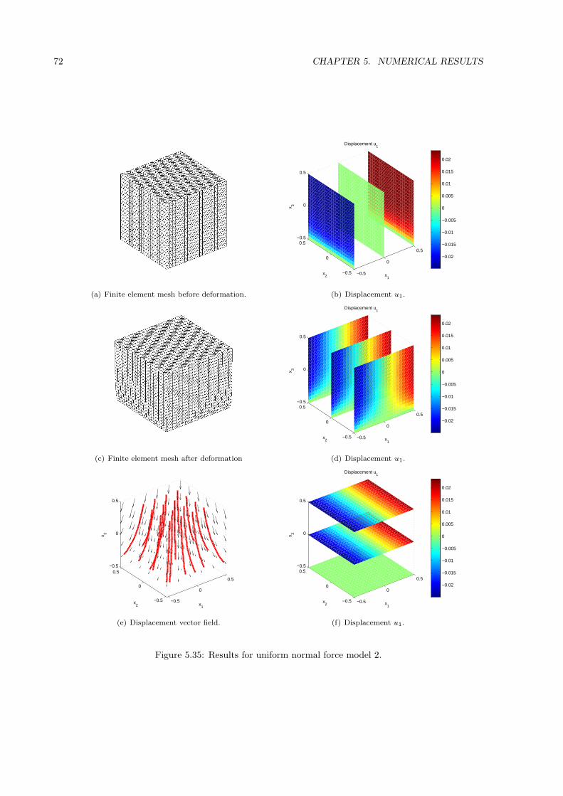
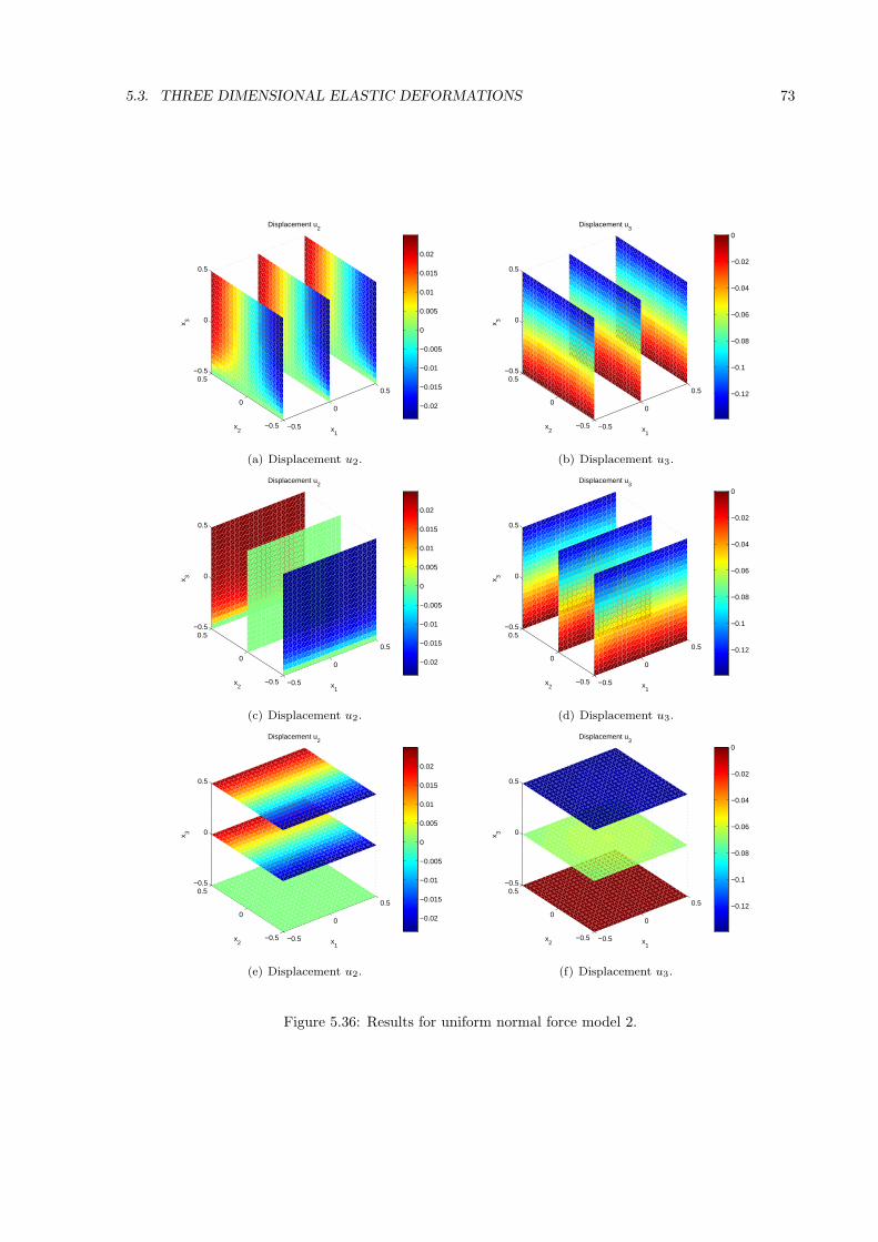
5.35 Results for uniform normal force model 2. . . . . . . . . . . . . . . . . . . . . . . . . . . . 725.36 Results for uniform normal force model 2. . . . . . . . . . . . . . . . . . . . . . . . . . . . 735.37 Results for normal point force model 1. . . . . . . . . . . . . . . . . . . . . . . . . . . . . 755.38 Results for normal point force model 1. . . . . . . . . . . . . . . . . . . . . . . . . . . . . 765.39 Results for normal point force model 2. . . . . . . . . . . . . . . . . . . . . . . . . . . . . 785.40 Results for normal point force model 2. . . . . . . . . . . . . . . . . . . . . . . . . . . . . 795.41 Topology for odd-even decomposition for three dimensional mesh. . . . . . . . . . . . . . . 80
Heat treatment and manufacturing of aluminum alloys is a complex operation that has several factorsthat influence the usability of the object after metalworking. The influence of most of these factors havebeen studied and achieved by a process of trial and error. Examples of such factors are the temperature,deformations and radiation. Although the experimentally achieved results are useful, they are onlyperformed on a particular ally or in a particular setting, which as a results implies that the results can befalse for other alloys and settings. To resolve this problem a mathematical model for the influence of thesefactors could be proposed. Until recently only statistical models have been proposed, tested and verified,but these models only investigate the influences of the temperature on the alloy. Therefore a model basedon possible exact solutions of a problem can me more useful and and possibly can be combined with othermodels, such as the those for the deformation within an alloy due to exterior or interior forces. It seemslikely that these models will consist of several partial differential equations, which can be solved exact orwith numerical methods.
This document will focus on the factor regarding nucleation and growth of particles in aluminum alloysduring rolling or extrusion, since the presence and size of particles can influences the characteristics ofthe aluminum alloy object. Nucleation and growth of the particles will be modeled by following thesame reasoning as Myhr and Grong [7]. Metalworking of an object will be done by means of stress-strainrelations which will result in (in)elastic deformation models.
In this paper we show that the model proposed by Myhr and Grong [7] is correct, but also can beimproved by use of other time integration methods. We will also derive a elastic deformation model, forwhich will be shown that numerically obtained results are congruent with physics.
The remainder of this document is structured as follows. First an introduction to the field of met-allurgy is given. Chapter 3 will derive and state the models for particle nucleation and growth and forelastic deformations. The next chapter will reproduce part of the results from [7], compare differenttime integration methods and discuss results from numerical simulation of the elastic deformation model.Finally some conclusions will be drawn and follow-up work will be stated.
1
2 CHAPTER 1. INTRODUCTION
Chapter 2
Preliminaries in metallurgy
This chapter deals with the basic metallurgy concepts that are required to understand the behavior ofalloys during equilibrium and when changing to equilibrium. We begin with a short introduction aboutthe ordering of alloys. Then a discussion is presented about the thermodynamical behavior of alloysand the related phase diagrams. Next the diffusional concepts related to alloys are stated. Thereaftertransformations due to diffusion are discussed. Finally some information is presented about metalworkingtechniques. The information presented in this chapter mostly originates from [9], especially Chapters 1,2 and 5.
2.1 Metal alloys
Although the term alloy or metal alloy is unambiguous, one can still order these alloys by their properties.Such an ordering can be made on the solvent metal, but also on the number of components of the alloy.If using the solvent metal for ordering one can distinct the following twenty groups:
Aluminum Gold Mercury TinBismuth Indium Nickel UraniumCobalt Iron Potassium ZincCopper Lead Silver ZirconiumGallium Magnesium Titanium Rare earth metals
Another common ordering uses the number of components in the alloy. Although any alloy uninten-tionally contains all the elements from the periodic table, only traces of most elements are found. If weneglect those elements of which only traces are present, we can number the components of the alloy bydecreasing weight percentage or another factor. If only one alloy element is present besides the solventmetal, we speak of binary alloys. Likewise a ternary alloy consist of two alloy elements besides the solventmetal. Quaternary alloys consist of three alloy elements and the solvent metal. Alloys with more thenthree alloy elements do not have a specific name, which is why we call it complex alloys.
Besides the ordering on the number of components of an alloy there exist a subordering for the ternary,quaternary and more complex alloys. This ordering is based on the interaction of the alloy elements witheach other. Assume we have a ternary alloy with alloy elements that have the intension to bond with eachother. As a result we can view this alloy as a binary alloy, since each nuclei that will form, consists of oneelement, namely the combination of the two original elements. A ternary alloy with this property will becalled a quasi-binary alloy. Likewise a distinction can be made in quaternary and complexer alloys.
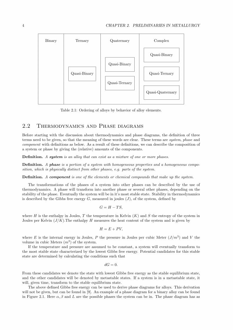
Using the last ordering by number of components and the subordering by behavior of the alloy elementsthe overview in Table 2.1 is gained.
3
4 CHAPTER 2. PRELIMINARIES IN METALLURGY
Binary Ternary Quaternary Complex
Quasi-Binary
Quasi-Binary
Quasi-Binary Quasi-Ternary
Quasi-Ternary
Quasi-Quaternary
Table 2.1: Ordering of alloys by behavior of alloy elements.
2.2 Thermodynamics and Phase diagrams
Before starting with the discussion about thermodynamics and phase diagrams, the definition of threeterms need to be given, so that the meaning of these words are clear. These terms are system, phase andcomponent with definitions as below. As a result of these definitions, we can describe the composition ofa system or phase by giving the (relative) amounts of the components.
Definition. A system is an alloy that can exist as a mixture of one or more phases.
Definition. A phase is a portion of a system with homogeneous properties and a homogeneous compo-
sition, which is physically distinct from other phases, e.g. parts of the system.
Definition. A component is one of the elements or chemical compounds that make up the system.
The transformations of the phases of a system into other phases can be described by the use ofthermodynamics. A phase will transform into another phase or several other phases, depending on thestability of the phase. Eventually the system will be in it’s most stable state. Stability in thermodynamicsis described by the Gibbs free energy G, measured in joules (J), of the system, defined by
G = H − TS,
where H is the enthalpy in Joules, T the temperature in Kelvin (K) and S the entropy of the system inJoules per Kelvin (J/K).The enthalpy H measures the heat content of the system and is given by
H = E + PV,
where E is the internal energy in Joules, P the pressure in Joules per cubic Meter (J/m3) and V thevolume in cubic Meters (m3) of the system.
If the temperature and pressure are assumed to be constant, a system will eventually transform tothe most stable state characterized by the lowest Gibbs free energy. Potential candidates for this stablestate are determined by calculating the conditions such that
dG = 0.
From these candidates we denote the state with lowest Gibbs free energy as the stable equilibrium state,and the other candidates will be denoted by metastable states. If a system is in a metastable state, itwill, given time, transform to the stable equilibrium state.
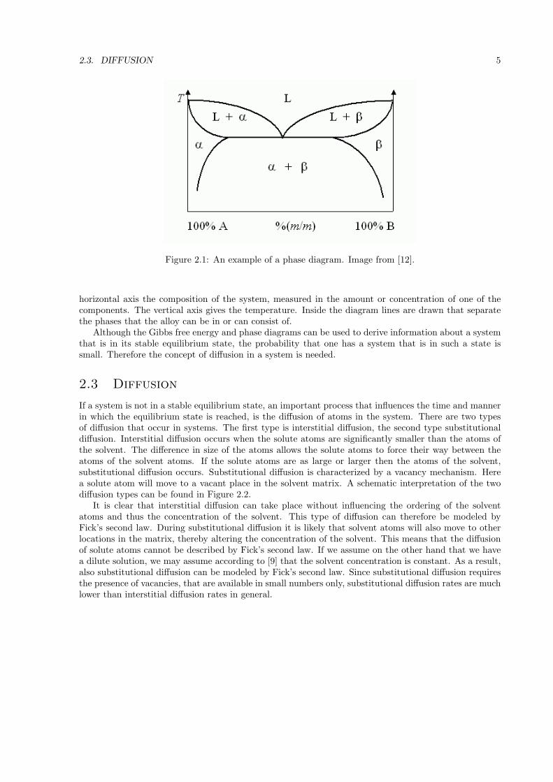
The above defined Gibbs free energy can be used to derive phase diagrams for alloys. This derivationwill not be given, but can be found in [9]. An example of a phase diagram for a binary alloy can be foundin Figure 2.1. Here α, β and L are the possible phases the system can be in. The phase diagram has as
2.3. DIFFUSION 5
Figure 2.1: An example of a phase diagram. Image from [12].
horizontal axis the composition of the system, measured in the amount or concentration of one of thecomponents. The vertical axis gives the temperature. Inside the diagram lines are drawn that separatethe phases that the alloy can be in or can consist of.
Although the Gibbs free energy and phase diagrams can be used to derive information about a systemthat is in its stable equilibrium state, the probability that one has a system that is in such a state issmall. Therefore the concept of diffusion in a system is needed.
2.3 Diffusion
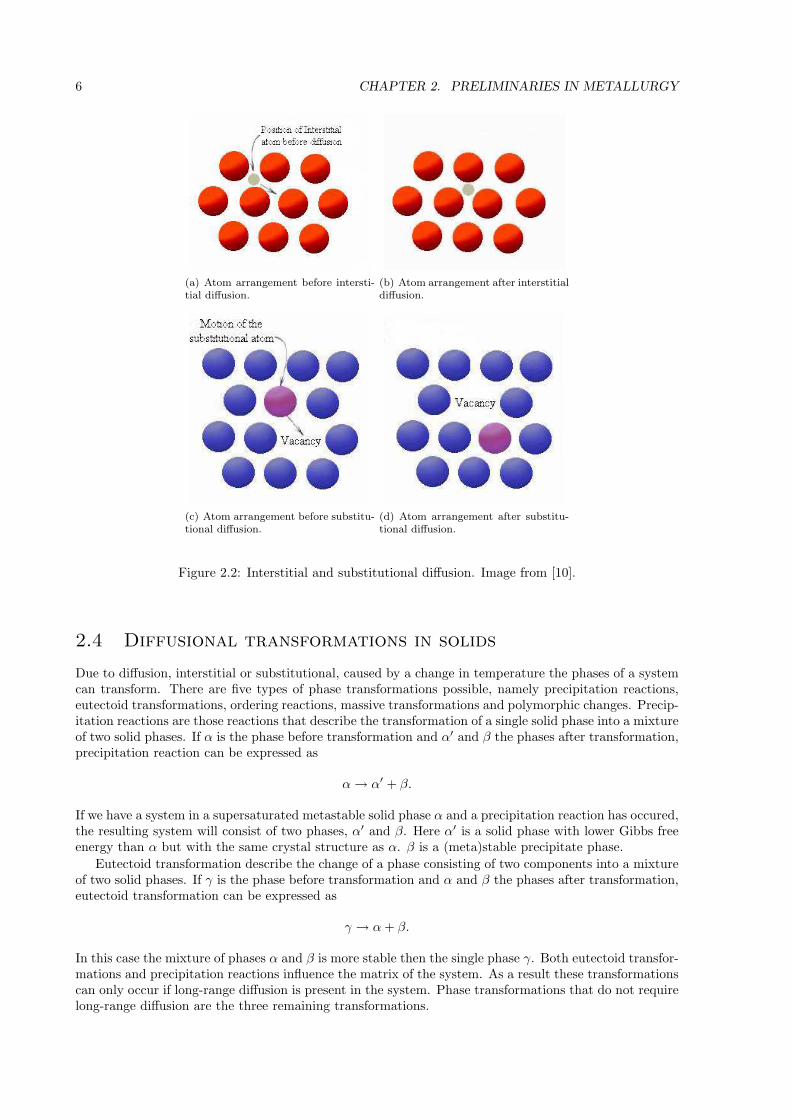
If a system is not in a stable equilibrium state, an important process that influences the time and mannerin which the equilibrium state is reached, is the diffusion of atoms in the system. There are two typesof diffusion that occur in systems. The first type is interstitial diffusion, the second type substitutionaldiffusion. Interstitial diffusion occurs when the solute atoms are significantly smaller than the atoms ofthe solvent. The difference in size of the atoms allows the solute atoms to force their way between theatoms of the solvent atoms. If the solute atoms are as large or larger then the atoms of the solvent,substitutional diffusion occurs. Substitutional diffusion is characterized by a vacancy mechanism. Herea solute atom will move to a vacant place in the solvent matrix. A schematic interpretation of the twodiffusion types can be found in Figure 2.2.
It is clear that interstitial diffusion can take place without influencing the ordering of the solventatoms and thus the concentration of the solvent. This type of diffusion can therefore be modeled byFick’s second law. During substitutional diffusion it is likely that solvent atoms will also move to otherlocations in the matrix, thereby altering the concentration of the solvent. This means that the diffusionof solute atoms cannot be described by Fick’s second law. If we assume on the other hand that we havea dilute solution, we may assume according to [9] that the solvent concentration is constant. As a result,also substitutional diffusion can be modeled by Fick’s second law. Since substitutional diffusion requiresthe presence of vacancies, that are available in small numbers only, substitutional diffusion rates are muchlower than interstitial diffusion rates in general.
6 CHAPTER 2. PRELIMINARIES IN METALLURGY
(a) Atom arrangement before intersti-tial diffusion.
(b) Atom arrangement after interstitialdiffusion.
(c) Atom arrangement before substitu-tional diffusion.
(d) Atom arrangement after substitu-tional diffusion.
Figure 2.2: Interstitial and substitutional diffusion. Image from [10].
2.4 Diffusional transformations in solids
Due to diffusion, interstitial or substitutional, caused by a change in temperature the phases of a systemcan transform. There are five types of phase transformations possible, namely precipitation reactions,eutectoid transformations, ordering reactions, massive transformations and polymorphic changes. Precip-itation reactions are those reactions that describe the transformation of a single solid phase into a mixtureof two solid phases. If α is the phase before transformation and α′ and β the phases after transformation,precipitation reaction can be expressed as
α → α′ + β.
If we have a system in a supersaturated metastable solid phase α and a precipitation reaction has occured,the resulting system will consist of two phases, α′ and β. Here α′ is a solid phase with lower Gibbs freeenergy than α but with the same crystal structure as α. β is a (meta)stable precipitate phase.
Eutectoid transformation describe the change of a phase consisting of two components into a mixtureof two solid phases. If γ is the phase before transformation and α and β the phases after transformation,eutectoid transformation can be expressed as
γ → α + β.
In this case the mixture of phases α and β is more stable then the single phase γ. Both eutectoid transfor-mations and precipitation reactions influence the matrix of the system. As a result these transformationscan only occur if long-range diffusion is present in the system. Phase transformations that do not requirelong-range diffusion are the three remaining transformations.
2.4. DIFFUSIONAL TRANSFORMATIONS IN SOLIDS 7
Ordering reactions describe the transformation of a single phase α to the single phase α′ and wherethe phase α has an disordered matrix structure and α′ a ordered matrix structure. Reactions of thesetypes can be expressed as
α(disordered) → α′(ordered).
If a phase transforms into several other phases that have different crystal structures than the originalphase, but with the same overall composition, a massive transformation has occurred. A simple exampleof this type of transformation can be described by the transformation
β → α.
In single component systems there can exist crystal structures that are stable in some temperatureranges. If the temperature changes in such a way that the present phase becomes unstable, a polymorphictransformation will occur. After this transformation the system will be in a stable phase with differentcrystal structure then the starting phase. Such a reaction can be described by
γ → α.
A schematic representation of the above discussed phase transformations can be found in Figure 2.3.
Figure 2.3: Examples of diffusional phase transformations. Image from [9].
In this thesis only phase transformations caused by precipitation reactions are modeled. These trans-formations are characterized by diffusional nucleation and growth. There are two types of nucleation,namely homogeneous and heterogeneous. The latter is the most occurring type and therefore will be usedto model the nucleation in a system. After nuclei are formed, the nuclei will grow or shrink. This growthwill also be modeled to describe the behavior of the system under time. The models for nucleation andgrowth will not be derived here, but can for example be found in [9].
8 CHAPTER 2. PRELIMINARIES IN METALLURGY
2.5 Metalworking techniques
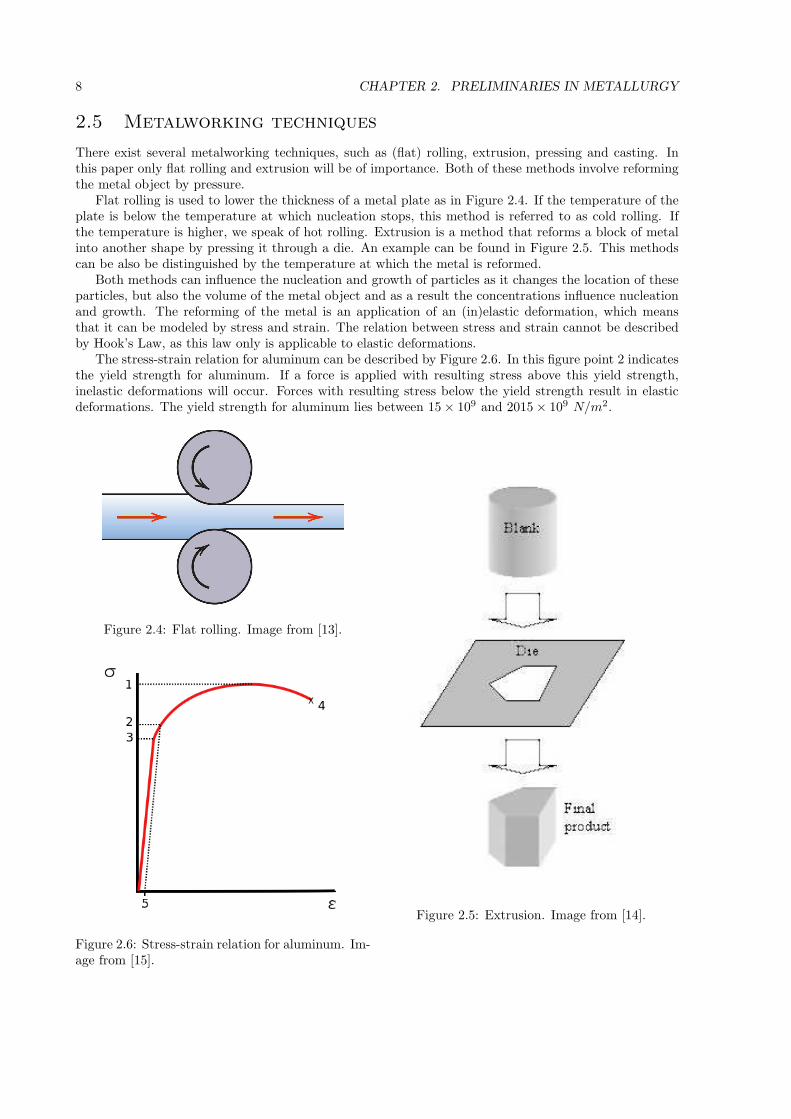
There exist several metalworking techniques, such as (flat) rolling, extrusion, pressing and casting. Inthis paper only flat rolling and extrusion will be of importance. Both of these methods involve reformingthe metal object by pressure.
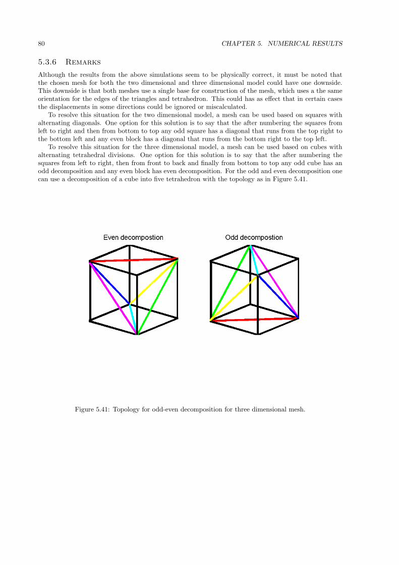
Flat rolling is used to lower the thickness of a metal plate as in Figure 2.4. If the temperature of theplate is below the temperature at which nucleation stops, this method is referred to as cold rolling. Ifthe temperature is higher, we speak of hot rolling. Extrusion is a method that reforms a block of metalinto another shape by pressing it through a die. An example can be found in Figure 2.5. This methodscan be also be distinguished by the temperature at which the metal is reformed.
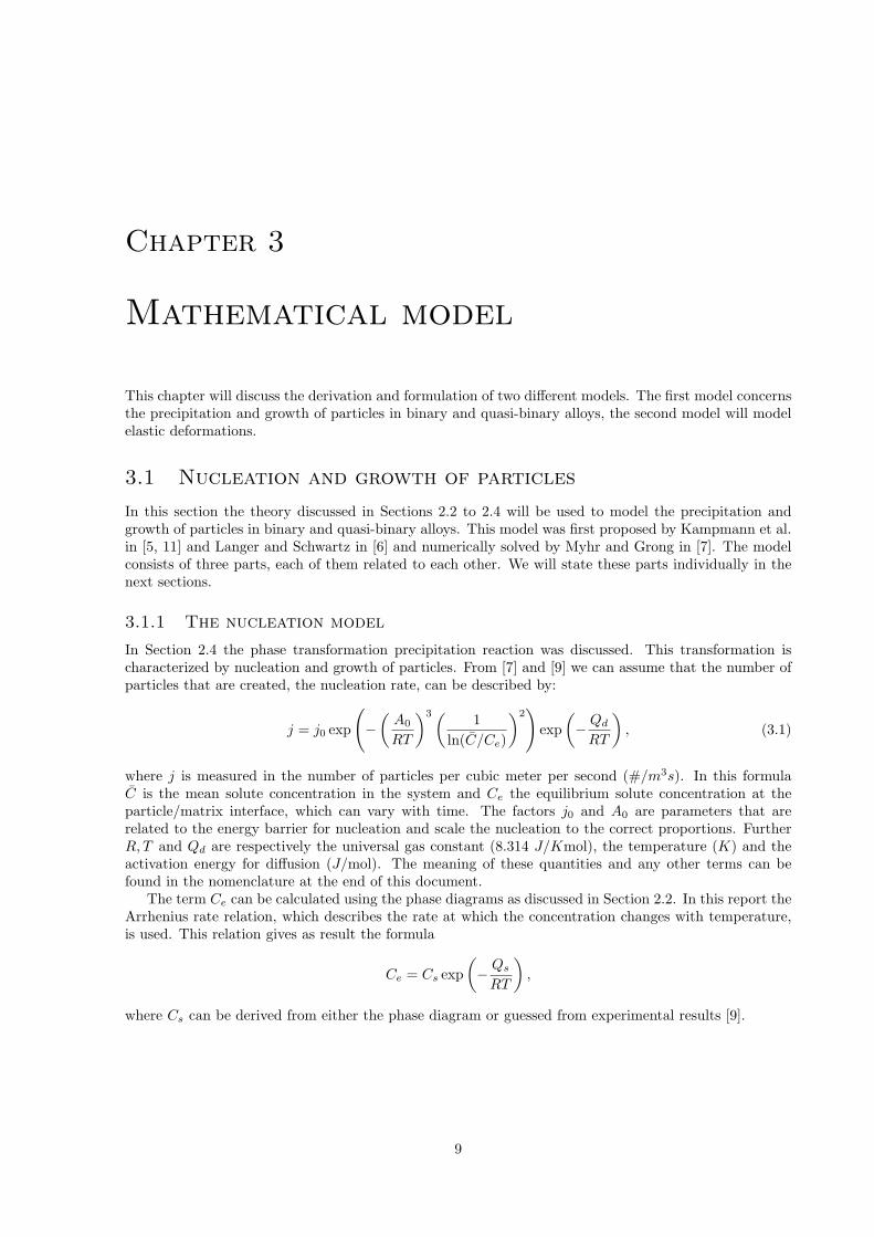
Both methods can influence the nucleation and growth of particles as it changes the location of theseparticles, but also the volume of the metal object and as a result the concentrations influence nucleationand growth. The reforming of the metal is an application of an (in)elastic deformation, which meansthat it can be modeled by stress and strain. The relation between stress and strain cannot be describedby Hook’s Law, as this law only is applicable to elastic deformations.
The stress-strain relation for aluminum can be described by Figure 2.6. In this figure point 2 indicatesthe yield strength for aluminum. If a force is applied with resulting stress above this yield strength,inelastic deformations will occur. Forces with resulting stress below the yield strength result in elasticdeformations. The yield strength for aluminum lies between 15 × 109 and 2015 × 109 N/m2.
Figure 2.4: Flat rolling. Image from [13].
Figure 2.6: Stress-strain relation for aluminum. Im-age from [15].
Figure 2.5: Extrusion. Image from [14].
Chapter 3
Mathematical model
This chapter will discuss the derivation and formulation of two different models. The first model concernsthe precipitation and growth of particles in binary and quasi-binary alloys, the second model will modelelastic deformations.
3.1 Nucleation and growth of particles
In this section the theory discussed in Sections 2.2 to 2.4 will be used to model the precipitation andgrowth of particles in binary and quasi-binary alloys. This model was first proposed by Kampmann et al.in [5, 11] and Langer and Schwartz in [6] and numerically solved by Myhr and Grong in [7]. The modelconsists of three parts, each of them related to each other. We will state these parts individually in thenext sections.
3.1.1 The nucleation model
In Section 2.4 the phase transformation precipitation reaction was discussed. This transformation ischaracterized by nucleation and growth of particles. From [7] and [9] we can assume that the number ofparticles that are created, the nucleation rate, can be described by:
j = j0 exp
(
−(
A0
RT
)3(1
ln(C/Ce)
)2)
exp
(
− Qd
RT
)
, (3.1)
where j is measured in the number of particles per cubic meter per second (#/m3s). In this formulaC is the mean solute concentration in the system and Ce the equilibrium solute concentration at theparticle/matrix interface, which can vary with time. The factors j0 and A0 are parameters that arerelated to the energy barrier for nucleation and scale the nucleation to the correct proportions. FurtherR, T and Qd are respectively the universal gas constant (8.314 J/Kmol), the temperature (K) and theactivation energy for diffusion (J/mol). The meaning of these quantities and any other terms can befound in the nomenclature at the end of this document.
The term Ce can be calculated using the phase diagrams as discussed in Section 2.2. In this report theArrhenius rate relation, which describes the rate at which the concentration changes with temperature,is used. This relation gives as result the formula
Ce = Cs exp
(
− Qs
RT
)
,
where Cs can be derived from either the phase diagram or guessed from experimental results [9].
9
10 CHAPTER 3. MATHEMATICAL MODEL
3.1.2 The rate law
Besides a nucleation rate that predicts the number of new particles that will be created per second, thegrowth of the present particles will influence the precipitation reaction. For the sake of simplicity, weassume that a particle has a spherical shape, with radius r. For this particle its radius will change intime at the rate
v =dr
dt=
C − Ci
Cp − Ci
D
r, (3.2)
where Ci is the particle/matrix interface concentration and Cp the concentration of the solute of interestinside the particle. It can be shown that Ci can be related to the equilibrium concentration Ce, whichresults in
Ci = Ce exp
(
2σVm
rRT
)
. (3.3)
For each combination of possible concentrations Ce, C, there is a particle that will neither grow ordissolve. From (3.2) and (3.3) we can derive that this particle has radius
r∗ =2σVm
RT
(
ln
(
C
Ce
))−1
(3.4)
which we will call the critical particle radius of the system. From this result we can also conclude that vis negative for radii smaller than r∗ and that v is positive for radii larger than r∗. This means that thesmaller particles will dissolve and the larger will grow.
The diffusion coefficient D can be calculated by means of an exponential formula depending on Qd, Rand T and is given by
D = D0 exp
(
− Qd
RT
)
,
where D0 is derived from experimental results. For the derivation of this formula one is invited to readChapter 2 of [9].
3.1.3 The particle size distribution
During this study, we are interested in the number of particles in a certain system as a function of time.One tool to describe this is the use of a particle concentration function. If we denote this concentrationby N with the definition that N(r, t) indicates the number op particles per cubic meter with particleradius between r−∆r/2 and r + ∆r/2 at time t, we may derive a model for N . ∆r is a numerical value,which can be interpreted as the size of a numerical control interval.
Let Ω = (r, r + ∆r) ⊆ [0,∞) be an arbitrary domain. Let F be the flux of transport of particlesover radii from this domain. If we assume that F has positive orientation, the flow of particles into Ω isdefined by F (r). Similar the flow out of Ω equals F (r + ∆r). The change of particles with radii fromΩ can also be due to a source term S. As a result, the change in time of the number of particles withradius from Ω can be expressed as
∆r∂N
∂t= F (r) − F (r + ∆r) + ∆rS.
Dividing by ∆r and letting ∆r tend to zero, we arrive with the use of the definition of the partialderivative at
∂N
∂t= −∂F
∂r+ S.
By definition, the flux F is defined as the number of particles that cross a certain boundary, normalizedby the area of that boundary. Since we are working in one dimension, we can say that this area equals1. We also formally know the rate at which the particles ‘move’, i.e. grow, namely v. This means thatthe flux F is given by F = Nv. Substituting this relation into the derived partial differential equation,results in
∂N
∂t= −∂(Nv)
∂r+ S. (3.5)
3.1. NUCLEATION AND GROWTH OF PARTICLES 11
In the field of metallurgy one is often not interested in the number of particles per cubic meter (N),but in the particle size distribution function φ. To simplify things N is calculated numerically, afterwhich φ can be determined by the relation ∆riφ(ri, t) = N(ri, t) where ri is the center of a numericalcontrol volume and ∆ri the size of this control interval.
3.1.4 The complete model for the particle distribution
Although we have formulated three formal expressions about the nucleation and growth of particles, wedo not have a closed system yet. Closing this system requires the definition of the source term S in (3.5)and the definition of boundary and initial conditions for N .
We will start with defining the source term S. This term represents the number of particles thatnucleate per second per cubic meter. In Section 3.1.1 we have formulated the function j, that has thissame meaning. So a logical step is to relate S to j, but S = j is not useful, since then the overallproduction over the real axis can become infinitely large. Research by Kampmann et al. [5] has indicatedthat the particles that are being formed have a radius that is slightly larger then the critical radius r∗.Let ∆r∗ be a small positive number and denote by r∗ +∆r∗ the radius of particles that are being formed.Now we can formally say that S is given by
S(r, t) =
j(t) if r = r∗ + ∆r∗,
0 otherwise.(3.6)
Although we now have defined the source term S, yet no relation between j and N has been given.This relation can be made easily if we define the mean concentration C as a function of N . In the abovesection we have formally defined the function φ as the size distribution function, which is related to Nand will be used in the needed relation.
First define the particle volume fraction f as
f(t) =
∫
∞
0
4
3πr3φdr. (3.7)
Note that f is dimensionless. If no particles are present, we can easily see that f = 0 and that C = C0,where C0 is the concentration of the solute in the overall system. This concentration is assumed to beknown for each system. If on the other hand particles are present, the weight percentage of the solutein the particles is given by Cpf . As a result the concentration of solute not in the particles, C, can beexpressed by
C =C0 − Cpf
1 − f. (3.8)
Using equations (3.7) and (3.8) to obtain j and S we have related S to our function N , which wasneeded to close the system. A fortunate result of the derived relation, is that we also have found a relationbetween v and N , by means of C.
On inspecting the partial differential equation (3.5), we see that at most one initial condition and atmost one boundary condition is needed. The initial condition is of the form
N(r, 0) = N0(r),
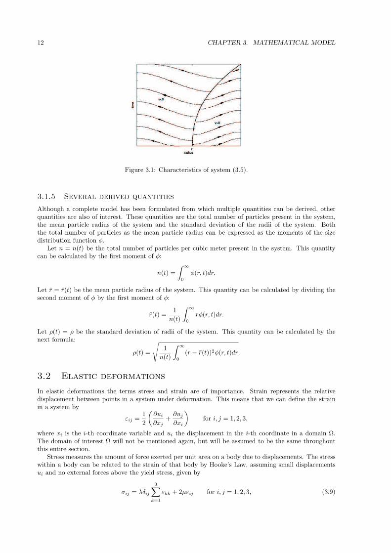
where N0 is a known positive function or identically zero. If we investigate the characteristics of thesystem, we see that these can be divided into to regions, to the left of r∗ and to the right of r∗. Thecharacteristics plane with the division line r∗ can be seen in Figure 3.1. The region left of r∗ has anegative growth rate v, to the right a positive growth rate v. Due to these characteristics, no boundarycondition need to be specified.
We now formulated a closed system that can predict the number of particles per cubic meter in analloy. This system is given by
∂N
∂t= −∂(Nv)
∂r+ S for r ∈ [0,∞), t ∈ (0,∞),
N(r, 0) = N0(r) for r ∈ [0,∞).
Note that this is a non-linear partial differential equation due to the relations between N, v and S.
12 CHAPTER 3. MATHEMATICAL MODEL
Figure 3.1: Characteristics of system (3.5).
3.1.5 Several derived quantities
Although a complete model has been formulated from which multiple quantities can be derived, otherquantities are also of interest. These quantities are the total number of particles present in the system,the mean particle radius of the system and the standard deviation of the radii of the system. Boththe total number of particles as the mean particle radius can be expressed as the moments of the sizedistribution function φ.
Let n = n(t) be the total number of particles per cubic meter present in the system. This quantitycan be calculated by the first moment of φ:
n(t) =
∫
∞
0
φ(r, t)dr.
Let r = r(t) be the mean particle radius of the system. This quantity can be calculated by dividing thesecond moment of φ by the first moment of φ:
r(t) =1
n(t)
∫
∞
0
rφ(r, t)dr.
Let ρ(t) = ρ be the standard deviation of radii of the system. This quantity can be calculated by thenext formula:
ρ(t) =
√
1
n(t)
∫
∞
0
(r − r(t))2φ(r, t)dr.
3.2 Elastic deformations
In elastic deformations the terms stress and strain are of importance. Strain represents the relativedisplacement between points in a system under deformation. This means that we can define the strainin a system by
εij =1
2
(
∂ui
∂xj+
∂uj
∂xi
)
for i, j = 1, 2, 3,
where xi is the i-th coordinate variable and ui the displacement in the i-th coordinate in a domain Ω.The domain of interest Ω will not be mentioned again, but will be assumed to be the same throughoutthis entire section.
Stress measures the amount of force exerted per unit area on a body due to displacements. The stresswithin a body can be related to the strain of that body by Hooke’s Law, assuming small displacementsui and no external forces above the yield stress, given by
σij = λδij
3∑
k=1
εkk + 2µεij for i, j = 1, 2, 3, (3.9)
3.2. ELASTIC DEFORMATIONS 13
where δij is the Kronecker delta, λ the bulk modulus of the system and µ the shear modulus. The lattertwo moduli are also known as the Lamee constants.
Both λ and µ are related to the Young’s modulus E and the Possion’s ratio ν by the formulas
λ =Eν
(1 − 2ν)(ν + 1)
µ =E
2(ν + 1).
Any body under elastic deformation obeys Newton’s Second Law, which states that the sum of allforces acting an a body equals the mass of that body multiplied with the acceleration. If b is a vectorcontaining all internal body forces per unit volume, the sum of the forces is given by
∇ · σ + b,
per unit volume, with
σ =
σ11 σ12 σ13
σ21 σ22 σ23
σ31 σ32 σ33
.
The acceleration within the system is defined as
∂2u
∂t2
where u = (u1, u2, u3)T . As a result the force balance yields per unit volume
ρm∂2u
∂t2= ∇ · σ + b, (3.10)
with ρm the density of the material.Using the definitions and relations above, the last equation gives a system for the displacements
ui, i = 1, 2, 3 and is given by1:
ρm∂2u1
∂t2= λ
∂
∂x1(∇ · u) + µ
(
∇ ·(
∇u1 +∂u
∂x1
))
+ b1
ρm∂2u2
∂t2= λ
∂
∂x2(∇ · u) + µ
(
∇ ·(
∇u2 +∂u
∂x2
))
+ b2
ρm∂2u3
∂t2= λ
∂
∂x3(∇ · u) + µ
(
∇ ·(
∇u3 +∂u
∂x3
))
+ b3.
(3.11)
On the boundary of the system still conditions need to be imposed. From a physical point of viewthere are three things that can happen at a boundary Γ during rolling or extrusion:
• The boundary is fixed, so no displacements can occur.
• A force is exerted on the boundary.
• A free boundary on which no forces act, besides internal forces.
The first physical situation can be represented by mathematics by demanding
u = 0 on the boundary.
If a force is exerted, this can be described by
σ · n = f on the boundary,
with f = f(x, t) the force exerted and n the outward normal on the boundary. This boundary conditiongives boundary conditions for the spatial derivatives of ui, i = 1, 2, 3. If we take f ≡ 0, we arrive at the
1Assuming constant values for ρm, λ, µ.
14 CHAPTER 3. MATHEMATICAL MODEL
free boundary with no external forces. On a single region of the boundary the boundary condition canbe generalized. A formal representation of a possible boundary condition is thus of the form:
σ · n = f + [α1(ub1 − u1), α2(ub2 − u2), α3(ub3 − u3)]T . (3.12)
The initial conditions for (3.11) are determined by the initial state of the system. In most cases thisstate is the undeformed state of the system. This means that no displacements have occurred, but notthat the system is in rest. This means that we can impose the initial conditions
u(x, 0) = 0∂u
∂t(x, 0) = g(x),
(3.13)
on our system, where g(x) is any appropriate function, which can be integrated over the real numbers.In the special case of one dimension, we can rewrite (3.11) to
ρm∂2u
∂t2= (λ + 2µ)
∂2u
∂x2.
If we set
c2 =ρm
λ + 2µ,
we have the basic one dimensional wave equation
c2 ∂2u
∂t2=
∂2u
∂x2.
Assume for simplicity that u(x, t) satisfies inhomogeneous Dirichlet boundary conditions and theinitial conditions (3.13) and the one dimensional wave equation on (0, 1):
c2 ∂2u
∂t2= ∂2u
∂x2 on x ∈ (0, 1) and for t > 0,
u(0, t) = f1(t) for t > 0,u(1, t) = f2(t) for t > 0,u(x, 0) = 0 on x ∈ [0, 1],
∂u
∂t(x, 0) = g(x) on x ∈ [0, 1].
If we set
u(x, t) = v(x, t) + w(x),
and demand that v(x, t) satisfies the same initial conditions as u but with homogeneous boundary con-ditions and w(x, t) satisfies ∂2w/∂x2 = 0, we have the following to systems:
c2 ∂2v
∂t2=
∂2v
∂x2on x ∈ (0, 1) and for t > 0,
v(0, t) = 0 for t > 0,v(1, t) = 0 for t > 0,v(x, 0) = 0 on x ∈ [0, 1],
∂v
∂t(x, 0) = g(x) on x ∈ [0, 1],
and
∂2w∂x2 = 0 on x ∈ (0, 1) and for t > 0,
w(0) = f1(t) for t > 0,w(1) = f2(t) for t > 0.
The solution of the second system is easily determined and has time dependent constants:
w(x, t) = (f2(t) − f1(t))x + f1(t)x.
The first system has as solution
v(x, t) =∞∑
k=1
Bk sin(kπx) sin
(
kπt
c
)
,
3.2. ELASTIC DEFORMATIONS 15
where
Bk =c
2kπ
∫ 1
0
g(x) sin(kπx) dx.
If we investigate the behavior of Bk, we see that we have the property:
limc→0
Bk = 0,
which immediately results inlimc→0
v(x, t) = 0.
This means that if c is small, the only time dependence of the solution u(x, t) comes from the boundaryconditions. This means we can easily neglect the time dependence in the wave equation and say thatu(x, t) satisfies the system
d2u
dx2= 0 on x ∈ (0, 1)
u(0) = f1(t) for t > 0,u(1) = f2(t) for t > 0.
The result in the one dimensional case suggests that also in three dimensions the time dependencycan be neglected, which results in the differential equation
−λ∂
∂x1(∇ · u) − µ
(
∇ ·(
∇u1 +∂u
∂x1
))
= b1
−λ∂
∂x2(∇ · u) − µ
(
∇ ·(
∇u2 +∂u
∂x2
))
= b2
−λ∂
∂x3(∇ · u) − µ
(
∇ ·(
∇u3 +∂u
∂x3
))
= b3,
(3.14)
with boundary condition (3.12). Note that the boundary condition still has a possible time dependency,so that we can solve (3.14) at several time instances to simulate time behavior.
16 CHAPTER 3. MATHEMATICAL MODEL
Chapter 4
Numerical methods
This chapter will deal with the discretization of all models that have been formulated in the previouschapter. The model for nucleation and growth of particles will be discretized by the means of finitevolume methods, all other models by means of finite element methods.
4.1 Nucleation and growth of particles
This section will continue on the previous chapter by discretizing the partial differential equation (3.5)in time and place. We will start with the spatial discretization, after which a time integration andlinearization will take place. Then the discretization of the formulas needed will be given. Finally analgorithm will be given for solving our numerical scheme.
4.1.1 Spatial discretization
Integration over control interval
The spatial discretization of (3.5) will make use of the finite volume method, combined with an upwindscheme. To this end, we only calculate N on the region [rmin, rmax]. Now divide this region in M controlintervals Ωi with length ∆r and boundary Γi. Denote by ri the midpoint of interval Ωi and Ni as thevalue of N on r = ri.
Integration of the left-hand side of (3.5) over control interval Ωi gives
∫
Ωi
∂N
∂tdr =
d
dt
∫
Ωi
Ndr ≈ ∆rdNi
dt
Integration of the first term in the right-hand side of (3.5) gives
−∫
Ωi
∂(Nv)
∂rdr = − (Nv)|Γi
= −(
(Nv)i+1/2 − (Nv)i−1/2
)
≈ v+i−1/2Ni−1 − (v−
i−1/2 + v+i+1/2)Ni + v−
i+1/2Ni+1
with the uses of an upwind discretization, vi is short for v(ri, t) and the superscripts +,− stand for thepositive and negative parts respectively, which as been introduced to correctly use the upwind scheme.
Integration of the source term over Ωi, gives
∫
Ωi
Sdr ≈ ∆rSi
where Si is short for S(ri, t).
17
18 CHAPTER 4. NUMERICAL METHODS
Combining the discretizations we arrive at a matrix differential equation
d ~N(t)
dt= A(t) ~N(t) + ~S(t), (4.1)
where( ~N(t))i = Ni for i = 1, . . . , G − 1(A(t))ii = − 1
∆r (v−
i−1/2 + v+i+1/2) for i = 1, . . . , G − 1
(A(t))i,i−1 = 1∆r v+
i−1/2 for i = 2, . . . , G − 1
(A(t))i,i+1 = 1∆r v−
i+1/2 for i = 1, . . . , G − 1
(~S(t))i = Si for i = 1, . . . , G − 1,
and (A(t))ij = 0 if not defined above.
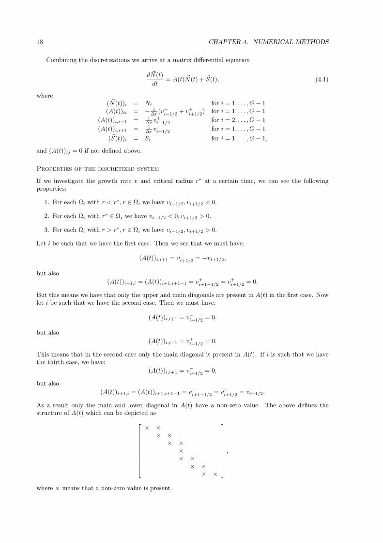
Properties of the discretized system
If we investigate the growth rate v and critical radius r∗ at a certain time, we can see the followingproperties:
1. For each Ωi with r < r∗, r ∈ Ωi we have vi−1/2, vi+1/2 < 0.
2. For each Ωi with r∗ ∈ Ωi we have vi−1/2 < 0, vi+1/2 > 0.
3. For each Ωi with r > r∗, r ∈ Ωi we have vi−1/2, vi+1/2 > 0.
Let i be such that we have the first case. Then we see that we must have:
(A(t))i,i+1 = v−
i+1/2 = −vi+1/2,
but also
(A(t))i+1,i = (A(t))i+1,i+1−1 = v+i+1−1/2 = v+
i+1/2 = 0.
But this means we have that only the upper and main diagonals are present in A(t) in the first case. Nowlet i be such that we have the second case. Then we must have:
(A(t))i,i+1 = v−
i+1/2 = 0,
but also
(A(t))i,i−1 = v+i−1/2 = 0.
This means that in the second case only the main diagonal is present in A(t). If i is such that we havethe thirth case, we have:
(A(t))i,i+1 = v−
i+1/2 = 0,
but also
(A(t))i+1,i = (A(t))i+1,i+1−1 = v+i+1−1/2 = v+
i+1/2 = vi+1/2.
As a result only the main and lower diagonal in A(t) have a non-zero value. The above defines thestructure of A(t) which can be depicted as
× ×× ×
× ××× ×
× ×× ×
,
where × means that a non-zero value is present.
4.1. NUCLEATION AND GROWTH OF PARTICLES 19
The time-dependent eigenvalues of A(t) can now easily be determined, since those are simply themain diagonal entries. To see this, assume we have a matrix as above, with elements aij . For simplicityassume we have a 5-matrix with the following structure:
a11 a12
a22 a23
a33
a43 a44
a54 a55
.
The characteristic polynomial of this matrix is:
∣
∣
∣
∣
∣
∣
∣
∣
∣
∣
a11 − λ a12
a22 − λ a23
a33 − λa43 a44 − λ
a54 a55 − λ
∣
∣
∣
∣
∣
∣
∣
∣
∣
∣
= (a11 − λ)
∣
∣
∣
∣
∣
∣
∣
∣
a22 − λ a23
a33 − λa43 a44 − λ
a54 a55 − λ
∣
∣
∣
∣
∣
∣
∣
∣
= (a11 − λ)(a22 − λ)
∣
∣
∣
∣
∣
∣
a33 − λa43 a44 − λ
a54 a55 − λ
∣
∣
∣
∣
∣
∣
= (a11 − λ)(a22 − λ)(a33 − λ)
∣
∣
∣
∣
a44 − λa54 a55 − λ
∣
∣
∣
∣
= (a11 − λ)(a22 − λ)(a33 − λ)(a44 − λ)(a55 − λ).
This means that the eigenvalues are the main diagonal elements and the i-th eigenvalue of A(t) is givenby
λi = −(v−
i−1/2 + v+i+1/2),
which is real and negative for all values of i. This result implicates that any time integration method canbe made stable as long as the stability region of this method contains (a part of) the negative real axis.
The order of the upwind method used in this section is O(∆r).
4.1.2 Time integration methods
The time integration of (4.1) will be done with several different methods. The methods discussed in thissection are the θ-method and two Diagonal Implicit Runge-Kutta methods (DIRK-methods) (see [4]).
The θ-method
This section will discuss the θ-method with 12 ≤ θ ≤ 1, resulting in an implicit method that is uncondi-
tionally stable for the system (4.1).
Let ~Nn be defined by~Nn = ~N(n∆t),
with ∆t the time-step size and all other variables likewise. Then we can approximate system (4.1) with
~Nn+1 = ~Nn + (1 − θ)∆t
∆rAn ~Nn + θ
∆t
∆rAn+1 ~Nn+1 + (1 − θ)∆t~Sn + θ∆t~Sn+1.
To be able to solve this system correctly we will linearize this system by approximating the matrixAn+1 and the vector ~Sn+1 by there values at the previous time step n. This gives
(
I − θ∆t
∆rAn
)
~Nn+1 =
(
I + (1 − θ)∆t
∆rAn
)
~Nn + ∆t~Sn. (4.2)
The discretization of the formulas in Chapter 3 will be down in a straightforward way when needed.The order of the θ-method is O(∆t) for θ 6= 1/2 and O(∆t2) for θ = 1/2.
20 CHAPTER 4. NUMERICAL METHODS
The first DIRK-method
All Runge-Kutta methods that exist are designed for solving the problem
w′(t) = F (t, w(t)),
for t > 0 and an initial condition w(0) = w0. Each method fulfills the general form
wn+1 = wn + ∆t
s∑
i=1
biF (tn + ci∆t, wni)
wni = wn + ∆ts∑
j=1
αijF (tn + cj∆t, wnj) for i = 1, . . . , s,
where αij , bi define the method and ci =∑s
j=1 αij . Each Runge-Kutta method can be thus characterizedby the values of αij , bi and ci, which can conveniently be expressed in a so-called Butcher array that hasthe form
c Abt =
c1 α11 · · · α1s
......
. . ....
cs αs1 · · · αss
b1 · · · bs
.
The first DIRK-method used is due to Nørsett [8] and Crouzeix [2] and is given by the Butcher array
γ γ 01 − γ 1 − 2γ γ
1/2 1/2,
with γ > 0. Applying this array to the general Runge-Kutta form gives
To be able to solve this system correctly we will linearize this system by approximating the matrix Aand vector ~S at other times than tn by there values at the time step n. This gives
~Nn+1 = ~Nn +∆t
2An(
~Nn1 + ~Nn2)
+ ∆t~Sn
~Nn1 = ~Nn + ∆tγ(
An ~Nn1 + ~Sn)
~Nn2 = ~Nn + ∆tAn(
(1 − 2γ) ~Nn1 + γ ~Nn2)
+ ∆t(1 − γ)~Sn.
The order of this method is O(∆t3) if γ = 12 ± 1
6
√3 and O(∆t2) otherwise. Also is known that this
method is unconditionally stable for (4.1) if γ ≥ 1/4.
4.1. NUCLEATION AND GROWTH OF PARTICLES 21
The second DIRK-method
The second DIRK-method used is attributed to Alt (1973) by Crouzeix and Raviart [3] and is given bythe Butcher array
0 0 0 02γ γ γ 01 b1 b2 γ
b1 b2 γ
,
with γ > 0, b1 = 32 − γ − 1
4γ and b2 = − 12 + 1
4γ . Applying this array to the general Runge-Kutta formgives
as numerical scheme.Applying this model to (4.1) and again linearizing the model as before, the following system results
~Nn+1 = ~Nn + ∆tAn(
b1~Nn1 + b2
~Nn2 + γ ~Nn3)
+ ∆t~Sn
~Nn1 = ~Nn
~Nn2 = ~Nn + ∆tγAn(
~Nn1 + ~Nn2)
+ 2∆tγ ~Sn
~Nn3 = ~Nn + ∆tAn(
b1~Nn1 + b2
~Nn2 + γ ~Nn3)
+ ∆t~Sn.
The order of this method is O(∆t3) if γ = 12 ± 1
6
√3 and O(∆t2) otherwise. Also is known that this
method is unconditionally stable for (4.1) if γ ≥ 1/4.
4.1.3 Solution algorithm
If we look at the structure of the matrix An, we see that it is a tri-diagonal matrix, which will onlybe altered on the diagonal or with a constant factor. A a result we can use the Tri-Diagonal MatrixAlgorithm, also known as the Thomas algorithm. For a system that has the form
b1 c1 0a2 b2 c2
a3 b3 .. . cn−1
0 an bn
x1
x2
.
.xn
=
d1
d2
.
.dn
,
with a1 = 0 and cn = 0, the algorithm starts with a first forward sweep, that modifies the coefficients ofthe system. This sweep produces the following coefficients with corresponding formula:
c′i =
ci
bi
for i = 1ci
bi−c′i−1
ai
for i = 2, . . . n
d′i =
di
bi
for i = 1di−d′
i−1ai
bi−c′i−1
ai
for i = 2, . . . n.
The system produced has the form:
1 c′1 01 c′2
1 .. c′n−1
0 1
x1
x2
.
.xn
=
d′1d′2..
d′n
.
22 CHAPTER 4. NUMERICAL METHODS
This system can be solved by a backward sweep defined by
xi =
d′n for i = n
d′i − c′ixi+1 for i = n − 1, . . . , 1.
A derivation of this algorithm can be found at [1].
4.2 Elastic deformations
To be able to derive the numerical scheme for the system (3.14), several steps have to be performed. Firsta weak formulation has to be found, after which an approximation of the solution should be imposed.The last step is to derive the element matrices and vectors. These steps will be performed on the threedimensional model, but first we will discuss the application of these steps on the two dimensional versionof (3.14).
4.2.1 Two dimensional model
The model
Although we have derived a three dimensional model, an understanding of this model can be obtainedby simulation of the corresponding two dimensional model. This model can be derived from (3.14) byassuming no dependency on x3 and that no displacements u3 occur. This reduces the model to:
−λ∂
∂x1(∇ · u) − µ
(
∇ ·(
∇u1 +∂u
∂x1
))
= b1
−λ∂
∂x2(∇ · u) − µ
(
∇ ·(
∇u2 +∂u
∂x2
))
= b2.(4.3)
∇ now refers to (∂/∂x1, ∂/∂x2)T .
The weak formulation
To obtain the weak formulation of (4.3) denote by vi(x, t), i = 1, 2 the test functions with vi = 0 on thoseparts of the boundary for which ui = 0. Instead of using the equations as in (4.3) to derive the weakformulation, we will use the equivalent system
−∇ · σ = b. (4.4)
Multiplying the i-th row of (4.4) with vi and integration over the domain Ω results in the system
−∫
Ω
(∇ · σ)i vi dΩ =
∫
Ω
bivi dΩ.
The first integral in this equation can be simplified by using the divergence theorem and the boundarycondition (3.12):
∫
Ω
(∇ · σ)i vi dΩ =
∫
Ω
(
∇ ·[
σi1
σi2
])
i
vi dΩ
= −∫
Ω
[
σi1
σi2
]
· ∇vi dΩ +
∫
Γ
([
σi1
σi2
]
· n)
vi dΓ
= −∫
Ω
[
σi1
σi2
]
· ∇vi dΩ +
∫
Γ
(fi + αi(ubi − ui)) vi dΓ.
This means we get the following weak formulation of (4.3) where the definition of σij should be filledin:
∫
Ω
[
σi1
σi2
]
· ∇vi dΩ + αi
∫
Γ
uivi dΓ =
∫
Ω
bivi dΩ +
∫
Γ
(fi + αiubi)vi dΓ for i = 1, 2. (4.5)
4.2. ELASTIC DEFORMATIONS 23
Galerkin’s method
Next we will apply Galerkin’s method on (4.5). Let ϕk(x), k = 1, 2, . . . by any appropriate set of basisfunctions on Ω. Now approximate ui by
ui(x, t) ≈n+nb∑
l=1
uilϕl(x),
where n+nb is the total number of internal grid points and boundary points and set vi = ϕk. Substitutioninto (4.5) results after manipulation and substitution of the definition of σij in
[
S11 S12
S21 S22
] [
u1
u2
]
=
[
q1
q2
]
, (4.6)
and using the Hooke’s Law (see equation (3.9)) gives:
∂(Sij)kl = δijµ
2∑
m=1
∫
Ω
∂ϕk
∂xm
∂ϕl
∂xmdΩ + λ
∫
Ω
∂ϕk
∂xi
∂ϕl
∂xjdΩ
+ µ
∫
Ω
∂ϕk
∂xj
∂ϕl
∂xidΩ + δijαi
∫
Γ
ϕkϕl dΓ for i, j = 1, 2 and for k, l = 1, . . . , n + nb
(qi)k = bi
∫
Ω
ϕk dΩ +
∫
Γ
fiϕk dΓ + αiubi
∫
Γ
ϕk dΓ for i = 1, 2 and for k = 1, . . . , n + nb.
Element matrices and vectors
This section will state the element matrices and vectors for internal elements and boundary elements ofthe domain Ω and boundary Γ. We choose as internal elements linear triangles and as a result linear linesas boundary elements. The Newton-Cotes quadrature for an internal element e with points xi, i = 1, . . . , 3is
∫
e
f dΩ =|∆|6
3∑
i=1
f(xi),
where |∆|/2 is the area of e and for a boundary element b
∫
b
f dΓ =l
2
2∑
i=1
f(xi),
where l is the length of b.The basis function ϕi can be represented by the formula
ϕi(x) = a0i +
[
a1i
a2i
]
· x,
where a0i , a
1i , a
2i can be solved from the equation
1 x11 x2
1
1 x12 x2
2
1 x13 x2
3
a0i
a1i
a2i
=
δi1
δi2
δi3
.
Using the above notations and quadratures we arrive for an internal element e at the element matricesand vectors:
(Seij)kl =
|∆|2
(
λaikaj
l + µajkai
l + δijµ2∑
m=1
amk am
l
)
for i, j = 1, 2 and for k, l = 1, 2, 3
(qei )k =
|∆|6
bi for i = 1, 2 and for k = 1, 2, 3,
24 CHAPTER 4. NUMERICAL METHODS
and for a boundary element b
(Sbij)kl = αiδklδij
l
2for i, j = 1, 2 and for k, l = 1, 2
(qbi )k =
l
2fi(xk) +
l
2αiubi for i = 1, 2 and for k = 1, 2.
4.2.2 Three dimensional model
The weak formulation
To obtain the weak formulation of (3.14) denote by vi(x, t), i = 1, 2, 3 the test functions with vi = 0 onthose parts of the boundary for which ui = 0. Instead of using the equations as in (3.14) to derive theweak formulation, we will use the equivalent system (3.10) in its time independent form:
−∇ · σ = b. (4.7)
Multiplying the i-th row of (4.7) with vi and integration over the domain Ω results in the system
−∫
Ω
(∇ · σ)i vi dΩ =
∫
Ω
bivi dΩ.
The second integral in this equation can be simplified by using the divergence theorem and the boundarycondition (3.12):
∫
Ω
(∇ · σ)i vi dΩ =
∫
Ω
∇ ·
σi1
σi2
σi3
i
vi dΩ
= −∫
Ω
σi1
σi2
σi3
· ∇vi dΩ +
∫
Γ
σi1
σi2
σi3
· n
vi dΓ
= −∫
Ω
σi1
σi2
σi3
· ∇vi dΩ +
∫
Γ
(fi + αi(ubi − ui)) vi dΓ.
This means we get the following weak formulation of (3.14) where the definition of σij should be filledin:
∫
Ω
σi1
σi2
σi3
· ∇vi dΩ + αi
∫
Γ
uivi dΓ =
∫
Ω
bivi dΩ +
∫
Γ
(fi + αiuib)vi dΓ for i = 1, 2, 3. (4.8)
Galerkin’s method
Next we will apply Galerkin’s method on (4.8). Let ϕk(x), k = 1, 2, . . . by any appropriate set of basisfunctions on Ω. Now approximate ui by
ui(x, t) ≈n+nb∑
l=1
uilϕl(x),
where n+nb is the total number of internal grid points and boundary points and set vi = ϕk. Substitutioninto (4.8) results after manipulation and substitution of the definition of σij in
S11 S12 S13
S21 S22 S23
S31 S32 S33
u1
u2
u3
=
q1
q2
q3
, (4.9)
4.2. ELASTIC DEFORMATIONS 25
and definitions:
(Sij)kl = δijµ
3∑
m=1
∫
Ω
∂ϕk
∂xm
∂ϕl
∂xmdΩ + λ
∫
Ω
∂ϕk
∂xi
∂ϕl
∂xjdΩ
+ µ
∫
Ω
∂ϕk
∂xj
∂ϕl
∂xidΩ + δijαi
∫
Γ
ϕkϕl dΓ for i, j = 1, 2, 3 and for k, l = 1, . . . , n + nb
(qi)k = bi
∫
Ω
ϕk dΩ +
∫
Γ
(fi + αiubi)ϕk dΓ for i = 1, 2, 3 and for k = 1, . . . , n + nb.
Element matrices and vectors
This section will state the element matrices and vectors for internal elements and boundary elements ofthe domain Ω and boundary Γ. We choose as internal elements linear tetrahedra and as a result lineartriangles as boundary elements. The Newton-Cotes quadrature for an internal element e with pointsxi, i = 1, . . . , 4 is
∫
e
f dΩ =|V |24
4∑
i=1
f(xi),
where |V |/6 is the volume of e and for a boundary element b
∫
b
f dΓ =|∆|6
3∑
i=1
f(xi),
where |∆|/2 is the area of b.The basis function ϕi can be represented by the formula
ϕi(x) = a0i +
a1i
a2i
a3i
· x,
where a0i , a
1i , a
2i , a
3i can be solved from the equation
1 x11 x2
1 x31
1 x12 x2
2 x32
1 x13 x2
3 x33
1 x14 x2
4 x34
a0i
a1i
a2i
a3i
=
δi1
δi2
δi3
δi4
.
Using the above notations and quadratures we arrive for an internal element e at the element matricesand vectors:
(Seij)kl = δijµ
|V |6
3∑
m=1
amk am
l + λ|V |6
aikaj
l + µ|V |6
ajkai
l for i, j = 1, 2, 3 and for k, l = 1, 2, 3, 4
(qei )k = bi
|V |24
for i = 1, 2, 3 and for k = 1, 2, 3, 4,
and for a boundary element b
(Sbij)kl = δklδijαi
|∆|6
for i, j = 1, 2, 3 and for k, l = 1, 2, 3
(qbi )k =
|∆|6
fi(xk) +|∆|6
αiubi for i = 1, 2, 3 and for k = 1, 2, 3.
26 CHAPTER 4. NUMERICAL METHODS
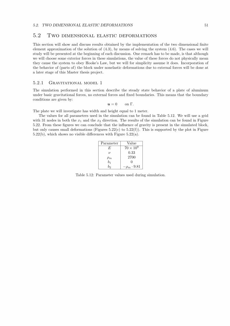
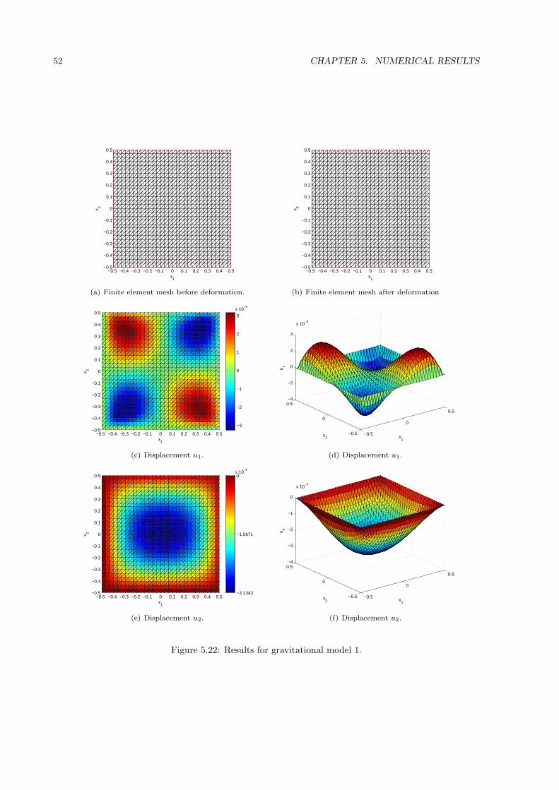
Chapter 5
Numerical results
This chapter has as purpose to state and discuss the results obtained from the numerical schemes inChapter 4.
5.1 Particle nucleation and growth
In this section simulations of the numerical schemes from Section 4.1 will be performed with severalapplications. The first application will serve as a test case for the quality of the mathematical modelformulated in Section 3.1. The second application will test the temperature dependence of the math-ematical model. These two test cases are the first two simulations carried out by Myhr and Grong in[7]. The other applications involve the determination of usable values for θ and γ used in the numericalschemes, but also to determine the difference in results and work for those values of θ and γ that can beused.
5.1.1 Context of the simulations from [7]
Both simulations carried out in the next sections will be concerned with the nucleation and growth ofparticles in a block of the aluminum alloy AA 6082, characterized by a nominal composition of 0.9 wt%silicium and 0.63 wt% magnesium. Due to the strong bond that exists between the atoms of the moleculMg2Si, this ternary alloy can be viewed as a quasi-binary alloy (see Section 2.1).
The values of the parameters needed in the simulation are copied from [7] and are given in Table 5.1.
Parameter ValueCp 63.4C0 0.63Cs 970D0 2.2 × 10⁻⁴
A0 1.622 × 10⁴
j0 9.66 × 1034
Qd 1.3 × 10⁵
Qs 4.7175 × 10⁴
σ 0.2Vm 3.95 × 10⁻⁵
∆r∗ 0.05r∗
Table 5.1: Value of parameters used during simulation. Data from [7].
We will assume that no particles are present at the beginning of our simulations, which means thatN(r, 0) = 0 for r ∈ (0,∞). The numerical values needed in the simulations can be found in Table 5.2.The value of ∆t will be stated for each simulation separately.
The numerical scheme in use here will be the θ-method with θ = 1, as this is the same scheme usedin [7].
27
28 CHAPTER 5. NUMERICAL RESULTS
Parameter Value∆r 0.95 × 10⁻¹⁰
G 100rmax 100 × 10−10
rmin 5 × 10⁻¹⁰
θ 1
Table 5.2: Value of numerical parameters used during simulation.
5.1.2 Long term behavior
The first simulation in [7] investigates the long term behavior of a system of the alloy AA 6082 underinfluence of a temperature of 180C or the equivalent temperature 453.15K. This method is calledprolonged artificial ageing in the field of metallurgy. During the simulation, we will let the time run from1 to 3 × 10⁶ seconds, which corresponds with approximately 35 days. The value of the time step will be∆t = 1. The results from the simulation can be found in Figures 5.1 and 5.2.
0 10 20 30 40 50 60 70 80 90 1000
1
2
3
4
5
6
7
8
9
10x 10
30 Size distribution functions
particle radius (Å)
size
dis
trib
utio
n (#
/m4 )
t=1.8e3t=5.9e3t=3.6e4t=4.1e5t=1.4e6t=2.5e6
Figure 5.1: Evolution of the size distribution function φ during prolonged artificial ageing at 180C.
From these results we can observe that the behavior of the system consists of three subsequent stages.For the first 103 seconds, we see that the particle volume fraction f and the mean concentration C areclose to constant. This means that the overall composition of the system does not change significantly.We also see that the nucleation rate j is also close to constant. This means that the overall numberof particles should increase at a reasonable constant rate, which is the case as can be seen from Figure5.2(b). Although the number of particles is increasing due to nucleation, the size of the particles remainssmall, since the mean radius r remains close to constant.
The next stage during the prolonged artificial ageing process is characterized by the growth of theparticles present. This stages last from approximately 103 seconds to about 2× 10⁴ seconds. During thisstage we see that the mean particles radius r increases rapidly and away from r∗, which is what shouldbe expected, since only particles larger than r∗ can increase. Due to the growth of the particles, theparticle volume fraction starts to increase sharply and the mean concentration and nucleation rate dropsignificantly. The latter is a result from the fact that C approaches the equilibrium concentration Ce
during this stage. Due to the low nucleation rate, the particle number density starts to stabilize.During the prolonged artificial ageing process the last stage is the coarsening stage. This stage is
characterized by the growth of larger particles at the expense of the smaller particles. This behavior canbe observed by the fairly constant values of the particle volume fraction and mean concentration. We
5.1. PARTICLE NUCLEATION AND GROWTH 29
100
102
104
106
0
0.1
0.2
0.3
0.4
0.5
0.6
0.7
0.8
0.9
1Particle volume fraction
part
icle
vol
ume
frac
tion
(%)
time (s)
(a) Evolution of the particle volume fraction f dur-ing prolonged artificial ageing at 180C.
100
102
104
106
1018
1019
1020
1021
1022
1023
Particle number density
time (s)
part
icle
num
ber
dens
ity (
#/m
3 )
(b) Evolution of the particle number density n dur-ing prolonged artificial ageing at 180C.
100
102
104
106
0
10
20
30
40
50
60
70
80
90Mean radius vs critical radius
time (s)
radi
us (
Å)
Mean radiusCriticial radius
(c) Evolution of the particle radii r and r∗ duringprolonged artificial ageing at 180C. Shaded areais the spread of radii around r by the standarddeviation ρ.
100
102
104
106
0
0.1
0.2
0.3
0.4
0.5
0.6
0.7Mean concentration vs equilibrium concentration
time (s)
conc
entr
atio
n (w
t%)
(d) Evolution of the concentrations C and Ce dur-ing prolonged artificial ageing at 180C.
100
102
104
106
10−120
10−100
10−80
10−60
10−40
10−20
100
1020
Nucleation rate
time (s)
nucl
eatio
n ra
te (
#/m
3 s)
(e) Evolution of the nucleation rate j during pro-longed artificial ageing at 180C.
Figure 5.2: Evolution of several quantities during prolonged ageing at 180 C.
30 CHAPTER 5. NUMERICAL RESULTS
also see that the mean radius and critical radius converges, but still continue to increase. Due to thedissolution of the smaller particles the number of particles starts to decrease, as can be observed fromthe particle number density.
Figure 5.1 contains two visible peaks that seem to be of an unphysical nature. If we investigate theheight and location of each peak at the relevant times, we see that the peaks are of the magnitude j/∆rat the location r∗ + ∆r∗. This means that the peaks are directly related to the nucleation term S of themodel (3.5). In the later stages of the simulation the peaks do not show, since then the magnitude ofj/∆r is significantly lower than that of φ at the location r∗ + ∆r∗.
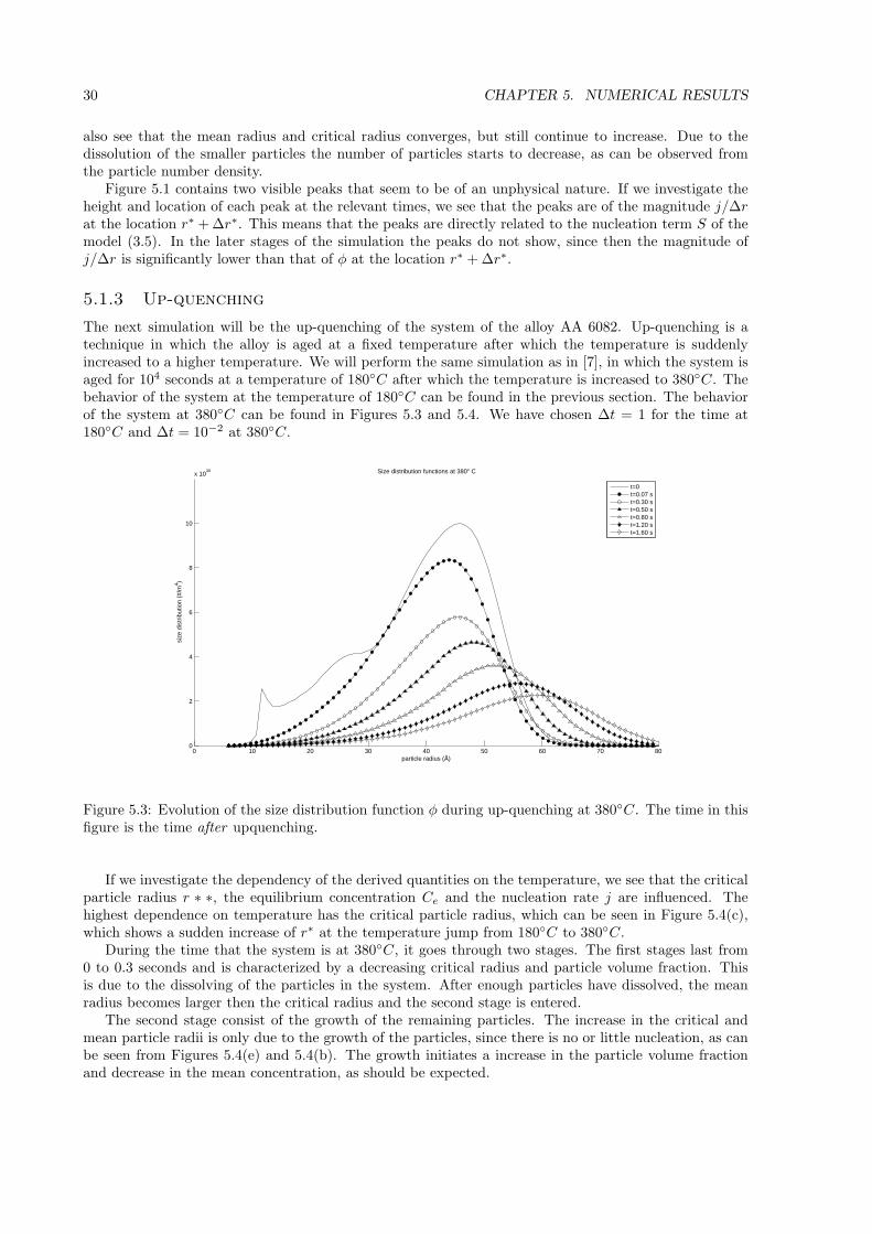
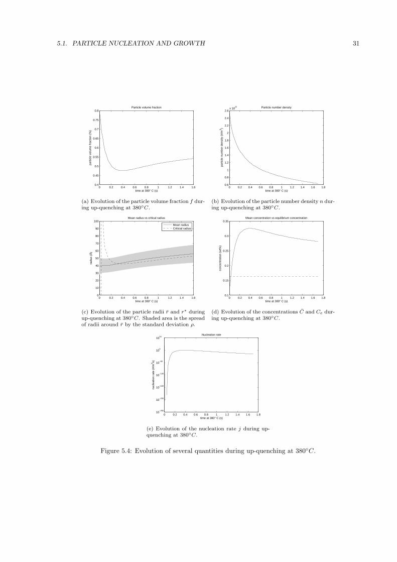
5.1.3 Up-quenching
The next simulation will be the up-quenching of the system of the alloy AA 6082. Up-quenching is atechnique in which the alloy is aged at a fixed temperature after which the temperature is suddenlyincreased to a higher temperature. We will perform the same simulation as in [7], in which the system isaged for 104 seconds at a temperature of 180C after which the temperature is increased to 380C. Thebehavior of the system at the temperature of 180C can be found in the previous section. The behaviorof the system at 380C can be found in Figures 5.3 and 5.4. We have chosen ∆t = 1 for the time at180C and ∆t = 10−2 at 380C.
0 10 20 30 40 50 60 70 800
2
4
6
8
10
x 1030 Size distribution functions at 380° C
particle radius (Å)
size
dis
trib
utio
n (#
/m4 )
t=0t=0.07 st=0.30 st=0.50 st=0.80 st=1.20 st=1.60 s
Figure 5.3: Evolution of the size distribution function φ during up-quenching at 380C. The time in thisfigure is the time after upquenching.
If we investigate the dependency of the derived quantities on the temperature, we see that the criticalparticle radius r ∗ ∗, the equilibrium concentration Ce and the nucleation rate j are influenced. Thehighest dependence on temperature has the critical particle radius, which can be seen in Figure 5.4(c),which shows a sudden increase of r∗ at the temperature jump from 180C to 380C.
During the time that the system is at 380C, it goes through two stages. The first stages last from0 to 0.3 seconds and is characterized by a decreasing critical radius and particle volume fraction. Thisis due to the dissolving of the particles in the system. After enough particles have dissolved, the meanradius becomes larger then the critical radius and the second stage is entered.
The second stage consist of the growth of the remaining particles. The increase in the critical andmean particle radii is only due to the growth of the particles, since there is no or little nucleation, as canbe seen from Figures 5.4(e) and 5.4(b). The growth initiates a increase in the particle volume fractionand decrease in the mean concentration, as should be expected.
5.1. PARTICLE NUCLEATION AND GROWTH 31
0 0.2 0.4 0.6 0.8 1 1.2 1.4 1.60.4
0.45
0.5
0.55
0.6
0.65
0.7
0.75
0.8Particle volume fraction
part
icle
vol
ume
frac
tion
(%)
time at 380° C (s)
(a) Evolution of the particle volume fraction f dur-ing up-quenching at 380C.
0 0.2 0.4 0.6 0.8 1 1.2 1.4 1.6 1.80.6
0.8
1
1.2
1.4
1.6
1.8
2
2.2
2.4
2.6x 10
22 Particle number density
part
icle
num
ber
dens
ity (
#/m
3 )
time at 380° C (s)
(b) Evolution of the particle number density n dur-ing up-quenching at 380C.
0 0.2 0.4 0.6 0.8 1 1.2 1.4 1.60
10
20
30
40
50
60
70
80
90
100Mean radius vs critical radius
time at 380° C (s)
radi
us (
Å)
Mean radiusCriticial radius
(c) Evolution of the particle radii r and r∗ duringup-quenching at 380C. Shaded area is the spreadof radii around r by the standard deviation ρ.
0 0.2 0.4 0.6 0.8 1 1.2 1.4 1.6 1.80.1
0.15
0.2
0.25
0.3
0.35Mean concentration vs equilibrium concentration
conc
entr
atio
n (w
t%)
time at 380° C (s)
(d) Evolution of the concentrations C and Ce dur-ing up-quenching at 380C.
0 0.2 0.4 0.6 0.8 1 1.2 1.4 1.6 1.810
−250
10−200
10−150
10−100
10−50
100
1050
Nucleation rate
time at 380° C (s)
nucl
eatio
n ra
te (
#/m
3 s)
(e) Evolution of the nucleation rate j during up-quenching at 380C.
Figure 5.4: Evolution of several quantities during up-quenching at 380C.
32 CHAPTER 5. NUMERICAL RESULTS
5.1.4 The θ-method
This section will discuss simulations performed with the θ-method for different values of θ. First thevalues of θ for which correct physical results can be obtained are determined. After this the results forthese values are discussed.
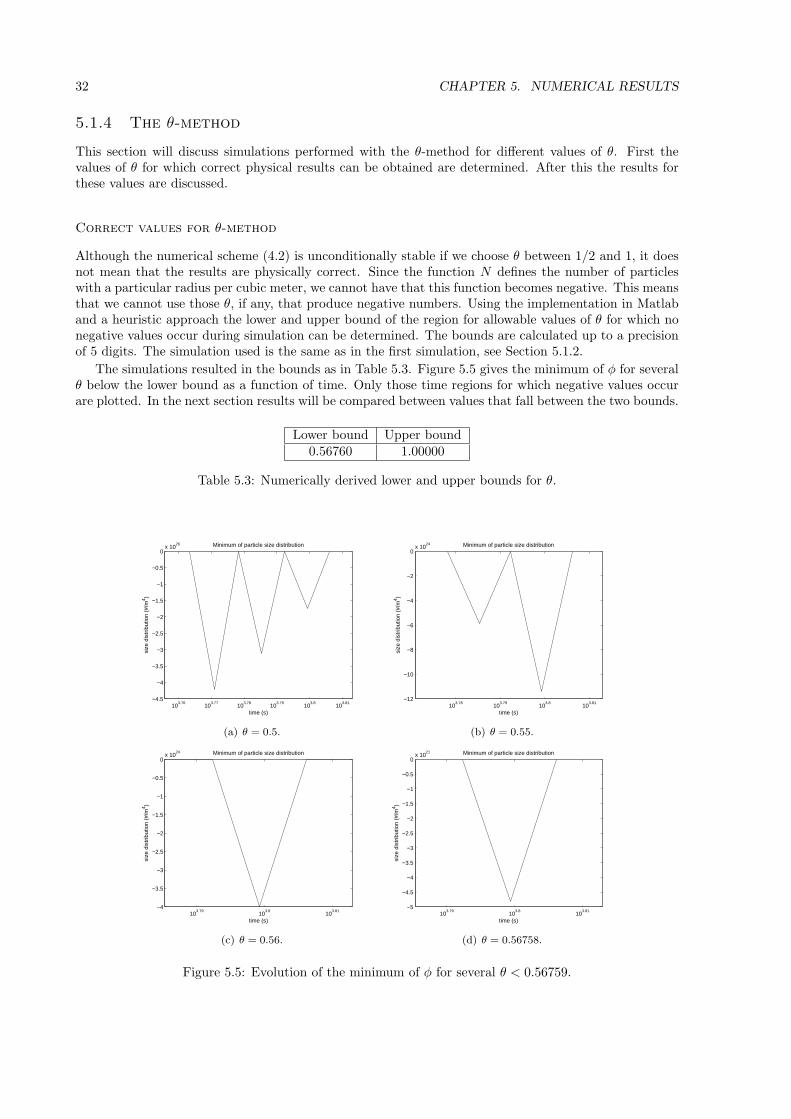
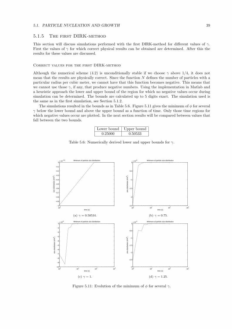
Correct values for θ-method
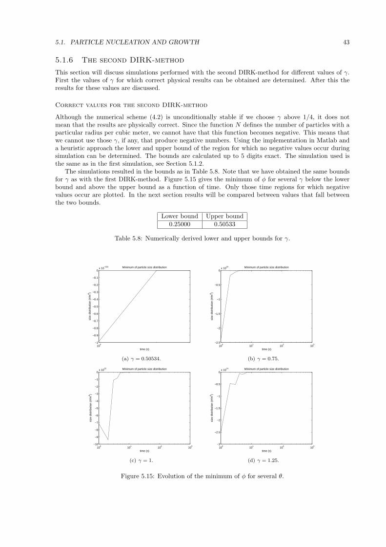
Although the numerical scheme (4.2) is unconditionally stable if we choose θ between 1/2 and 1, it doesnot mean that the results are physically correct. Since the function N defines the number of particleswith a particular radius per cubic meter, we cannot have that this function becomes negative. This meansthat we cannot use those θ, if any, that produce negative numbers. Using the implementation in Matlaband a heuristic approach the lower and upper bound of the region for allowable values of θ for which nonegative values occur during simulation can be determined. The bounds are calculated up to a precisionof 5 digits. The simulation used is the same as in the first simulation, see Section 5.1.2.
The simulations resulted in the bounds as in Table 5.3. Figure 5.5 gives the minimum of φ for severalθ below the lower bound as a function of time. Only those time regions for which negative values occurare plotted. In the next section results will be compared between values that fall between the two bounds.
Lower bound Upper bound0.56760 1.00000
Table 5.3: Numerically derived lower and upper bounds for θ.
103.76
103.77
103.78
103.79
103.8
103.81
−4.5
−4
−3.5
−3
−2.5
−2
−1.5
−1
−0.5
0x 10
26 Minimum of particle size distribution
time (s)
size
dis
trib
utio
n (#
/m4 )
(a) θ = 0.5.
103.78
103.79
103.8
103.81
−12
−10
−8
−6
−4
−2
0x 10
24 Minimum of particle size distribution
time (s)
size
dis
trib
utio
n (#
/m4 )
(b) θ = 0.55.
103.79
103.8
103.81
−4
−3.5
−3
−2.5
−2
−1.5
−1
−0.5
0x 10
24 Minimum of particle size distribution
time (s)
size
dis
trib
utio
n (#
/m4 )
(c) θ = 0.56.
103.79
103.8
103.81
−5
−4.5
−4
−3.5
−3
−2.5
−2
−1.5
−1
−0.5
0x 10
21 Minimum of particle size distribution
time (s)
size
dis
trib
utio
n (#
/m4 )
(d) θ = 0.56758.
Figure 5.5: Evolution of the minimum of φ for several θ < 0.56759.
5.1. PARTICLE NUCLEATION AND GROWTH 33
Comparison of θ-methods
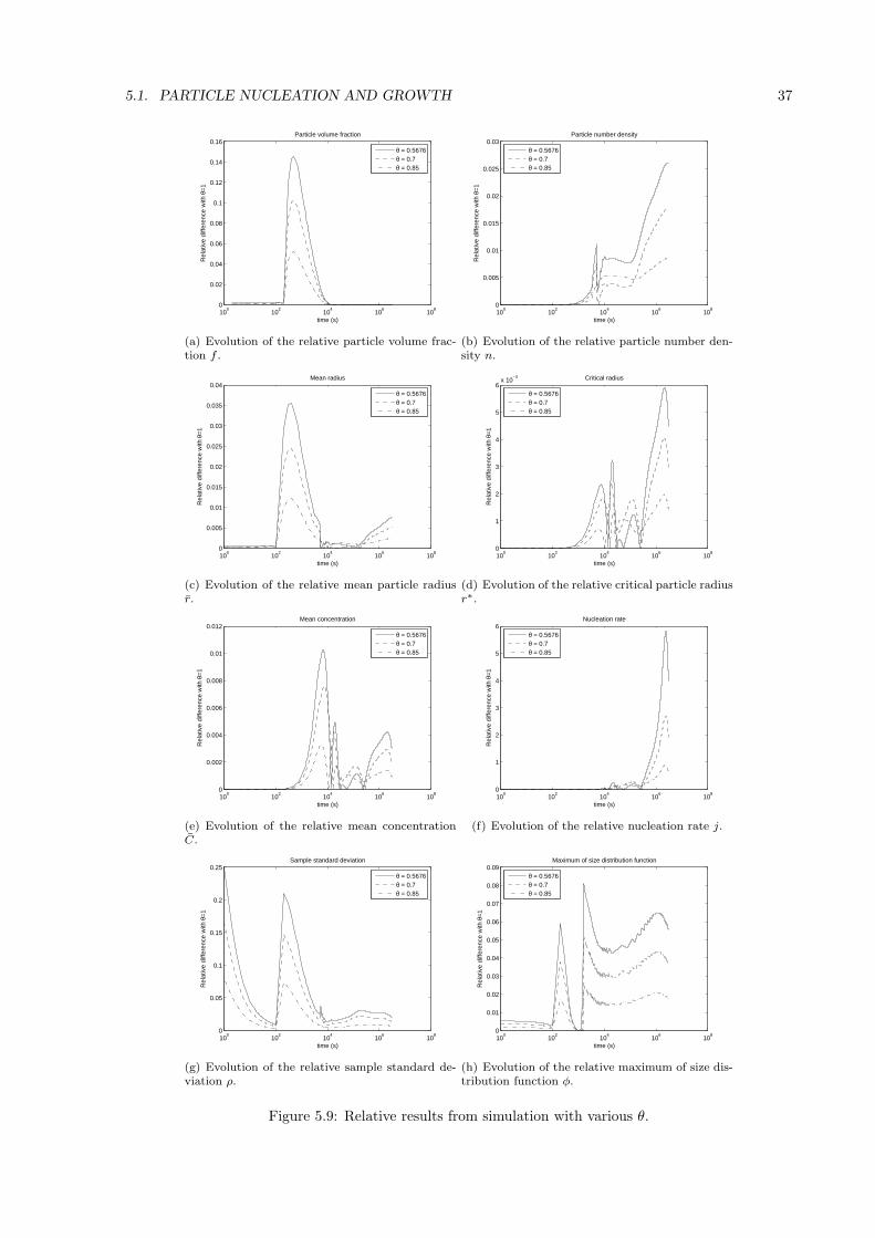
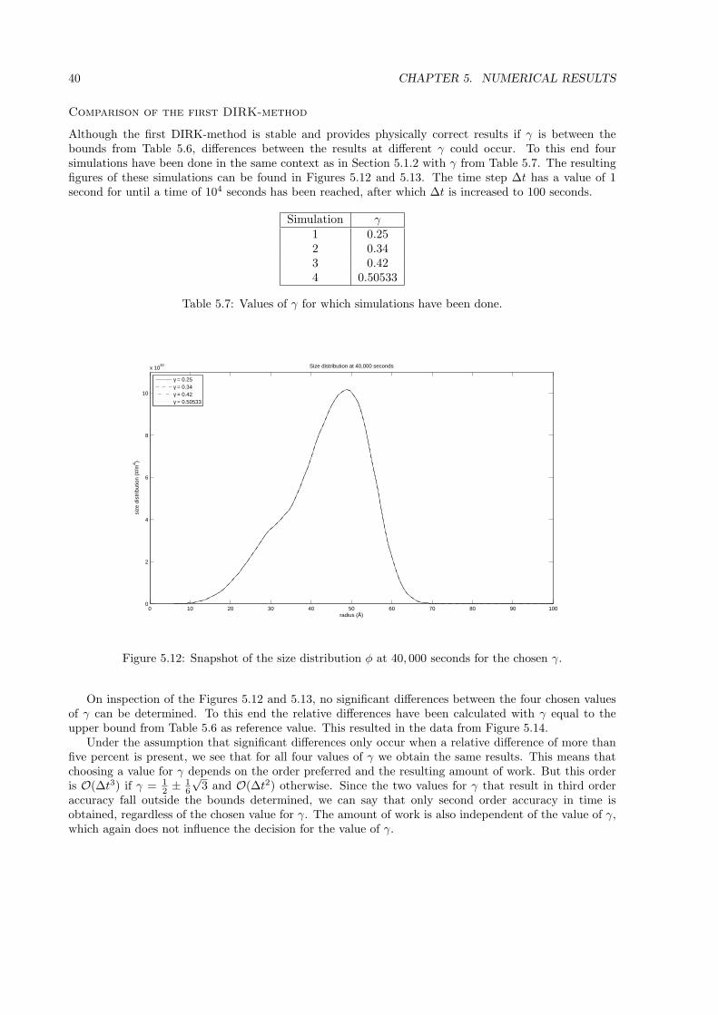
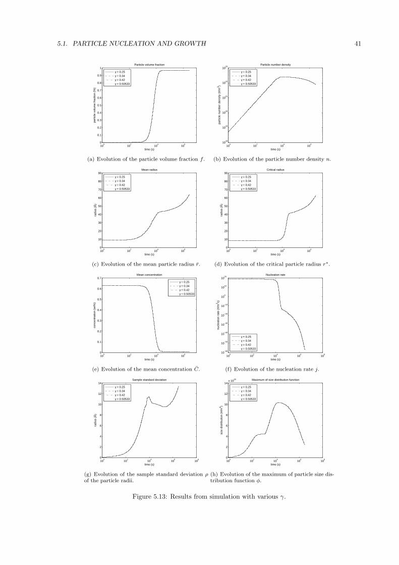
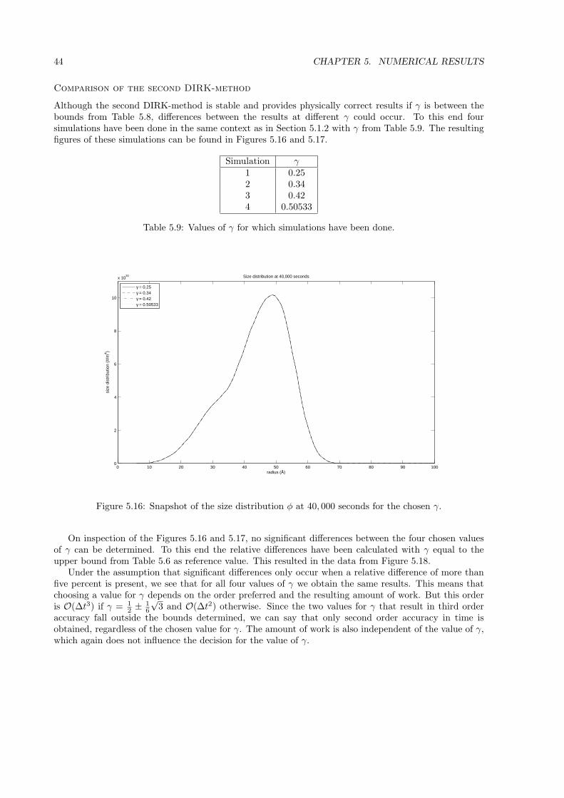
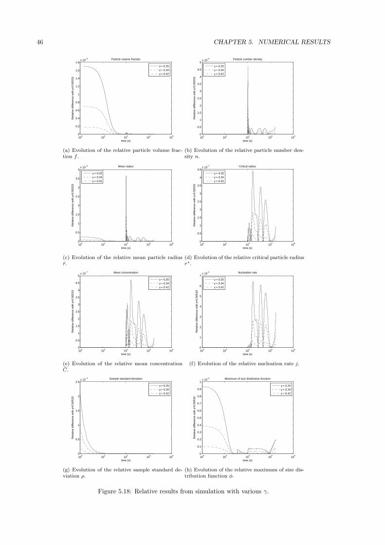
Although the θ-method is stable and provides physically correct results if θ is between the bounds fromTable 5.3, differences between the results at different θ could occur. To this end four simulations havebeen done in the same context as in Section 5.1.2 with θ from Table 5.4. The resulting figures of thesesimulations can be found in Figures 5.6 and 5.7.
Simulation θ1 0.56762 0.73 0.854 1
Table 5.4: Values of θ for which simulations have been done.
From the results obtained above some interesting conclusion can be drawn. The plots from Figure 5.6seem to indicate that the different values for θ do not influence the outcome of the model at all, whichmeans that choosing θ at a random value between the derived bounds gives the desired results. On theother hand, the plots in Figure 5.7 show that there is a difference in outcomes for the chosen values forθ. The difference between Figure 5.6 and Figure 5.7 can be explained by inspecting how the two plotsof Figure 5.7 differ. In the plot of the sample standard deviation ρ it can be seen that for increasing θ ρalso increases. This means that the plots of the size distribution function φ will be wider for increasingθ. The plot of the maximum of φ shows that for increasing θ the maximum will decrease. This meansthat the size distribution φ will be lower for increasing θ. One can verify this result with the plot fromFigure 5.8.
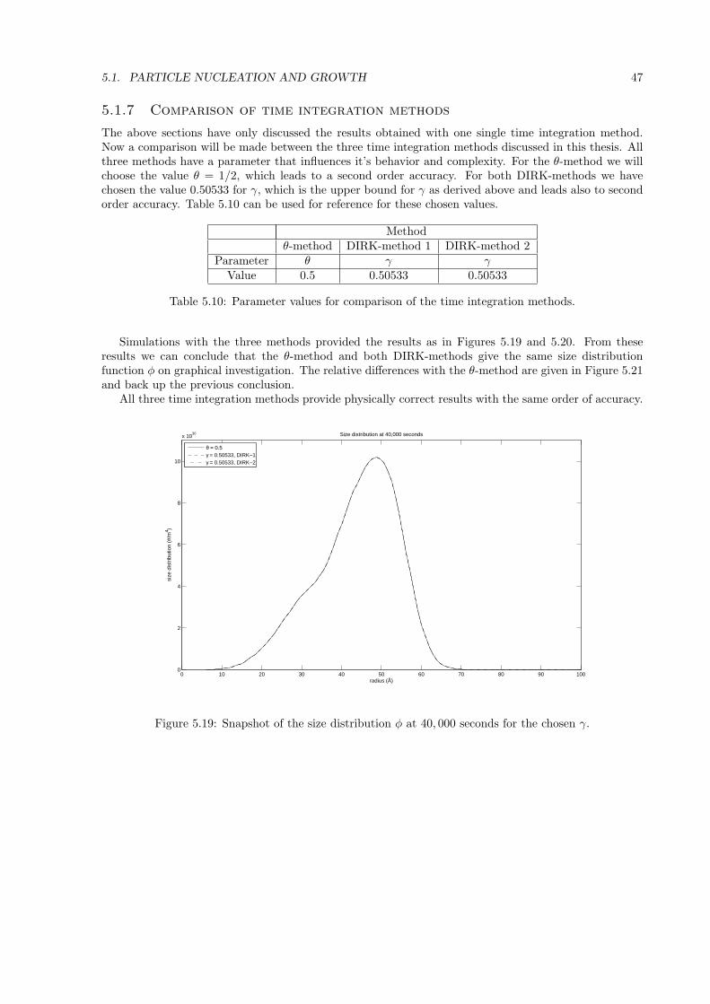
As a result the conclusion can be made that although the value of θ influences the shape of the sizedistribution slightly, it does not alter the outcome of the other functions, such as the particle volumefraction. This means that any θ between 0.5676 and 1 can be used. If we investigate the amount ofwork that must be done during simulation, we see that if θ 6= 1 one matrix multiplication and onematrix inversion is needed per time step. If θ = 1 only one matrix inversion is needed and no matrixmultiplications are needed. This means that choosing θ = 1 gives physically correct results at the lowestcosts. This gives as a result that the method used by Myhr and Grong [7] is mathematically preferable,which is the combination of an upwind spacial discretization, an implicit Euler time integration1 and alinearization in time.
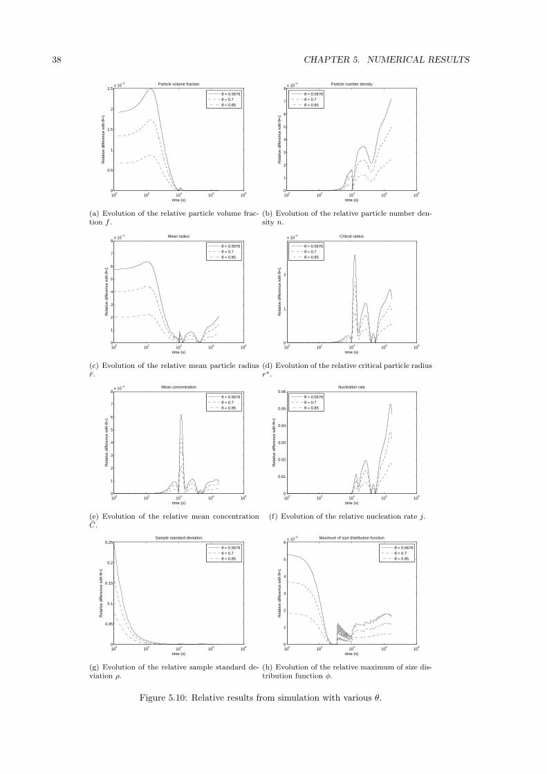
To further compare the different values for θ, we have computed the time-dependent differences ofthe output form different θ with the output for θ = 1 relative to the last. The chosen reference valueθ = 1 results from the fact that Myhr and Grong also use this value and their results have been assumedcorrect. The relative differences can be found in Figure 5.9.
If we say that a difference up to five percent is not relevant, the functions that come (temporarily)above this threshold, are the particle volume fraction f , the nucleation rate j, the sample standarddeviation ρ and the maximum of the size distribution function φ. The relative differences with θ = 1 forthe last two functions can be explained by the same behavior observed above. Recalling the function forthe particle volume fraction,
f(t) =
∫
∞
0
4
3πr3φdr,
we can explain the relative differences for this function. We can formally say that a wider size distributionfunction φ will have more large particles, which influences the overall particle volume fraction. Themoment in time at which the highest relative differences occur overlaps with the moment at which theparticle size distribution and particle volume fraction rapidly increase in magnitude. Although the relativedifferences for f occur, they are not visible for the mean concentration C. This can be explained by thefact that the formula for C involves a fraction with in the denominator and numerator the particle volumefraction, which cancels the effect of different f significantly. The peak in the relative differences for thenucleation rate j is six hundred percent, and occurs at the end of the algorithm. At this moment thevalue of j is of the order of 10−α with α ≥ 40, which is significantly small. This means that any deviationrelative to θ = 1 is of the order of 10−(α+2), which is neglectable in the overall system.
1This corresponds with the θ-method where θ = 1.
34 CHAPTER 5. NUMERICAL RESULTS
100
102
104
106
0
0.1
0.2
0.3
0.4
0.5
0.6
0.7
0.8
0.9
1Particle volume fraction
part
icle
vol
ume
frac
tion
(%)
time (s)
θ = 0.5676θ = 0.7θ = 0.85θ = 1
(a) Evolution of the particle volume fraction f .
100
102
104
106
1018
1019
1020
1021
1022
1023
Particle number density
time (s)
part
icle
num
ber
dens
ity (
#/m
3 )
θ = 0.5676θ = 0.7θ = 0.85θ = 1
(b) Evolution of the particle number density n.
100
102
104
106
0
10
20
30
40
50
60
70
80
90Mean radius
time (s)
radi
us (
Å)
θ = 0.5676θ = 0.7θ = 0.85θ = 1
(c) Evolution of the mean particle radius r.
100
102
104
106
0
10
20
30
40
50
60
70
80
90Critical radius
time (s)
radi
us (
Å)
θ = 0.5676θ = 0.7θ = 0.85θ = 1
(d) Evolution of the critical particle radius r∗.
100
102
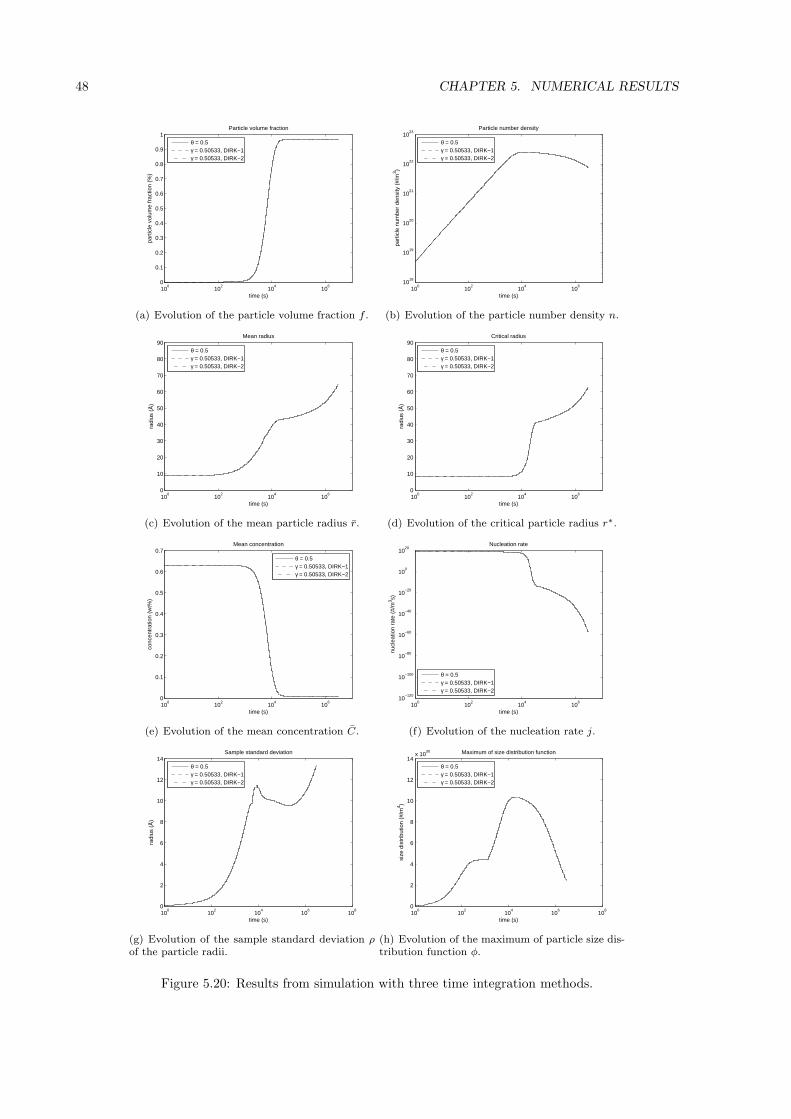
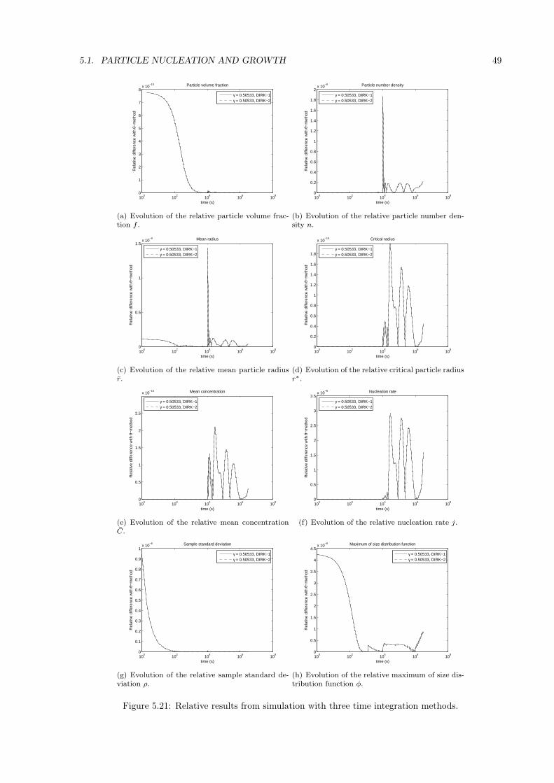
104
106
0
0.1
0.2
0.3
0.4
0.5
0.6
0.7Mean concentration
time (s)
conc
entr
atio
n (w
t%)
θ = 0.5676θ = 0.7θ = 0.85θ = 1
(e) Evolution of the mean concentration C.
100
102
104
106
108
10−60
10−50
10−40
10−30
10−20
10−10
100
1010
1020
Nucleation rate
time (s)
nucl
eatio
n ra
te (
#/m
3 s)
θ = 0.5676θ = 0.7θ = 0.85θ = 1
(f) Evolution of the nucleation rate j.
Figure 5.6: Results from simulation with various θ.
5.1. PARTICLE NUCLEATION AND GROWTH 35
100
101
102
103
104
105
106
107
0
2
4
6
8
10
12
14Sample standard deviation
time (s)
radi
us (
Å)
θ = 0.5676θ = 0.7θ = 0.85θ = 1
(a) Evolution of the sample standard deviation ρ of the particle radii.
100
101
102
103
104
105
106
107
0
2
4
6
8
10
12
14x 10
30 Maximum of size distribution function
time (s)
size
dis
trib
utio
n (#
/m4 )
θ = 0.5676θ = 0.7θ = 0.85θ = 1
(b) Evolution of the maximum of particle size distribution function φ.
Figure 5.7: Results from simulation with various θ.
36 CHAPTER 5. NUMERICAL RESULTS
0 10 20 30 40 50 60 70 80 90 1000
2
4
6
8
10
x 1030 Size distribution at 40,000 seconds
size
dis
trib
utio
n (#
/m4 )
radius (Å)
θ = 0.5676θ = 0.7θ = 0.85θ = 1
Figure 5.8: Snapshot of the size distribution φ at 40, 000 seconds for the chosen θ.
In some of the plots of Figure 5.9 a jump or sudden increase is visible at the time of 100 seconds. Atthis time the algorithm changes from a time step of one second to that of 100 seconds. To investigate theinfluence of this change in time step the simulation has be run with the change of the time step at thelater time of 10, 000 seconds. This gave the relative results as in Figure 5.10. From these figures we canconclude that now some jumps are present at the time of 10,000 seconds, which means that the change intime step influences the performance of the algorithm. Since the size of the jumps is lower in the lattersimulations, we will change the time step from 1 second to 100 seconds at the time of 10,000 seconds.
The change in the algorithm could have as effect that the bounds for θ change. Recalculation of thesebounds gave the values as in Table 5.5. This means we can conclude two things. First that the value andadaption of ∆t through time influences the physical outcome of the simulations. Second that a value of∆t = 1 is the best value to perform simulations.
Lower bound Upper bound0.50000 1.00000
Table 5.5: Numerically derived lower and upper bounds for θ.
The discussion about the relative differences for different values for θ confirms that although differencesoccur, these differences are neglectable. This supports the conclusion that choosing the value θ = 1 resultsin the correct physical values for the model and results in the least amount of work. But the order of thetime error is influenced by choosing θ = 1 since the time error is of order ∆t for all θ unequal to θ = 1/2and of order ∆t2 for θ = 1/2. This means that although choosing θ = 1/2 results in more computations,it will lead to more accurate results.
5.1. PARTICLE NUCLEATION AND GROWTH 37
100
102
104
106
108
0
0.02
0.04
0.06
0.08
0.1
0.12
0.14
0.16Particle volume fraction
Rel
ativ
e di
ffere
nce
with
θ=
1
time (s)
θ = 0.5676θ = 0.7θ = 0.85
(a) Evolution of the relative particle volume frac-tion f .
100
102
104
106
108
0
0.005
0.01
0.015
0.02
0.025
0.03Particle number density
time (s)
Rel
ativ
e di
ffere
nce
with
θ=
1
θ = 0.5676θ = 0.7θ = 0.85
(b) Evolution of the relative particle number den-sity n.
100
102
104
106
108
0
0.005
0.01
0.015
0.02
0.025
0.03
0.035
0.04Mean radius
time (s)
Rel
ativ
e di
ffere
nce
with
θ=
1
θ = 0.5676θ = 0.7θ = 0.85
(c) Evolution of the relative mean particle radiusr.
100
102
104
106
108
0
1
2
3
4
5
6x 10
−3 Critical radius
time (s)
Rel
ativ
e di
ffere
nce
with
θ=
1
θ = 0.5676θ = 0.7θ = 0.85
(d) Evolution of the relative critical particle radiusr∗.
100
102
104
106
108
0
0.002
0.004
0.006
0.008
0.01
0.012Mean concentration
time (s)
Rel
ativ
e di
ffere
nce
with
θ=
1
θ = 0.5676θ = 0.7θ = 0.85
(e) Evolution of the relative mean concentrationC.
100
102
104
106
108
0
1
2
3
4
5
6Nucleation rate
time (s)
Rel
ativ
e di
ffere
nce
with
θ=
1
θ = 0.5676θ = 0.7θ = 0.85
(f) Evolution of the relative nucleation rate j.
100
102
104
106
108
0
0.05
0.1
0.15
0.2
0.25Sample standard deviation
time (s)
Rel
ativ
e di
ffere
nce
with
θ=
1
θ = 0.5676θ = 0.7θ = 0.85
(g) Evolution of the relative sample standard de-viation ρ.
100
102
104
106
108
0
0.01
0.02
0.03
0.04
0.05
0.06
0.07
0.08
0.09Maximum of size distribution function
time (s)
Rel
ativ
e di
ffere
nce
with
θ=
1
θ = 0.5676θ = 0.7θ = 0.85
(h) Evolution of the relative maximum of size dis-tribution function φ.
Figure 5.9: Relative results from simulation with various θ.
38 CHAPTER 5. NUMERICAL RESULTS
100
102
104
106
108
0
0.5
1
1.5
2
2.5x 10
−3 Particle volume fraction
Rel
ativ
e di
ffere
nce
with
θ=
1
time (s)
θ = 0.5676θ = 0.7θ = 0.85
(a) Evolution of the relative particle volume frac-tion f .
100
102
104
106
108
0
1
2
3
4
5
6
7
8x 10
−4 Particle number density
time (s)
Rel
ativ
e di
ffere
nce
with
θ=
1
θ = 0.5676θ = 0.7θ = 0.85
(b) Evolution of the relative particle number den-sity n.
100
102
104
106
108
0
1
2
3
4
5
6
7
8x 10
−4 Mean radius
time (s)
Rel
ativ
e di
ffere
nce
with
θ=
1
θ = 0.5676θ = 0.7θ = 0.85
(c) Evolution of the relative mean particle radiusr.
100
102
104
106
108
0
1
2
x 10−4 Critical radius
time (s)
Rel
ativ
e di
ffere
nce
with
θ=
1
θ = 0.5676θ = 0.7θ = 0.85
(d) Evolution of the relative critical particle radiusr∗.
100
102
104
106
108
0
1
2
3
4
5
6
7
8x 10
−4 Mean concentration
time (s)
Rel
ativ
e di
ffere
nce
with
θ=
1
θ = 0.5676θ = 0.7θ = 0.85
(e) Evolution of the relative mean concentrationC.
100
102
104
106
108
0
0.01
0.02
0.03
0.04
0.05
0.06Nucleation rate
time (s)
Rel
ativ
e di
ffere
nce
with
θ=
1
θ = 0.5676θ = 0.7θ = 0.85
(f) Evolution of the relative nucleation rate j.
100
102
104
106
108
0
0.05
0.1
0.15
0.2
0.25Sample standard deviation
time (s)
Rel
ativ
e di
ffere
nce
with
θ=
1
θ = 0.5676θ = 0.7θ = 0.85
(g) Evolution of the relative sample standard de-viation ρ.
100
102
104
106
108
0
1
2
3
4
5
6x 10
−3 Maximum of size distribution function
time (s)
Rel
ativ
e di
ffere
nce
with
θ=
1
θ = 0.5676θ = 0.7θ = 0.85
(h) Evolution of the relative maximum of size dis-tribution function φ.
Figure 5.10: Relative results from simulation with various θ.
5.1. PARTICLE NUCLEATION AND GROWTH 39
5.1.5 The first DIRK-method
This section will discuss simulations performed with the first DIRK-method for different values of γ.First the values of γ for which correct physical results can be obtained are determined. After this theresults for these values are discussed.
Correct values for the first DIRK-method
Although the numerical scheme (4.2) is unconditionally stable if we choose γ above 1/4, it does notmean that the results are physically correct. Since the function N defines the number of particles with aparticular radius per cubic meter, we cannot have that this function becomes negative. This means thatwe cannot use those γ, if any, that produce negative numbers. Using the implementation in Matlab anda heuristic approach the lower and upper bound of the region for which no negative values occur duringsimulation can be determined. The bounds are calculated up to 5 digits exact. The simulation used isthe same as in the first simulation, see Section 5.1.2.
The simulations resulted in the bounds as in Table 5.6. Figure 5.11 gives the minimum of φ for severalγ below the lower bound and above the upper bound as a function of time. Only those time regions forwhich negative values occur are plotted. In the next section results will be compared between values thatfall between the two bounds.
Lower bound Upper bound0.25000 0.50533
Table 5.6: Numerically derived lower and upper bounds for γ.
100
−1
−0.9
−0.8
−0.7
−0.6
−0.5
−0.4
−0.3
−0.2
−0.1
0x 10
−222 Minimum of particle size distribution
time (s)
size
dis
trib
utio
n (#
/m4 )
(a) γ = 0.50534.
100
101
102
103
−2.5
−2
−1.5
−1
−0.5
0x 10
20 Minimum of particle size distribution
time (s)
size
dis
trib
utio
n (#
/m4 )
(b) γ = 0.75.
100
101
102
103
−10
−9
−8
−7
−6
−5
−4
−3
−2
−1
0x 10
22 Minimum of particle size distribution
time (s)
size
dis
trib
utio
n (#
/m4 )
(c) γ = 1.
100
101
102
103
−3
−2.5
−2
−1.5
−1
−0.5
0x 10
24 Minimum of particle size distribution
time (s)
size
dis
trib
utio
n (#
/m4 )
(d) γ = 1.25.
Figure 5.11: Evolution of the minimum of φ for several γ.
40 CHAPTER 5. NUMERICAL RESULTS
Comparison of the first DIRK-method
Although the first DIRK-method is stable and provides physically correct results if γ is between thebounds from Table 5.6, differences between the results at different γ could occur. To this end foursimulations have been done in the same context as in Section 5.1.2 with γ from Table 5.7. The resultingfigures of these simulations can be found in Figures 5.12 and 5.13. The time step ∆t has a value of 1second for until a time of 104 seconds has been reached, after which ∆t is increased to 100 seconds.
Simulation γ1 0.252 0.343 0.424 0.50533
Table 5.7: Values of γ for which simulations have been done.
0 10 20 30 40 50 60 70 80 90 1000
2
4
6
8
10
x 1030 Size distribution at 40,000 seconds
size
dis
trib
utio
n (#
/m4 )
radius (Å)
γ = 0.25γ = 0.34γ = 0.42γ = 0.50533
Figure 5.12: Snapshot of the size distribution φ at 40, 000 seconds for the chosen γ.
On inspection of the Figures 5.12 and 5.13, no significant differences between the four chosen valuesof γ can be determined. To this end the relative differences have been calculated with γ equal to theupper bound from Table 5.6 as reference value. This resulted in the data from Figure 5.14.
Under the assumption that significant differences only occur when a relative difference of more thanfive percent is present, we see that for all four values of γ we obtain the same results. This means thatchoosing a value for γ depends on the order preferred and the resulting amount of work. But this orderis O(∆t3) if γ = 1
2 ± 16
√3 and O(∆t2) otherwise. Since the two values for γ that result in third order
accuracy fall outside the bounds determined, we can say that only second order accuracy in time isobtained, regardless of the chosen value for γ. The amount of work is also independent of the value of γ,which again does not influence the decision for the value of γ.
5.1. PARTICLE NUCLEATION AND GROWTH 41
100
102
104
106
0
0.1
0.2
0.3
0.4
0.5
0.6
0.7
0.8
0.9
1Particle volume fraction
part
icle
vol
ume
frac
tion
(%)
time (s)
γ = 0.25γ = 0.34γ = 0.42γ = 0.50533
(a) Evolution of the particle volume fraction f .
100
102
104
106
1018
1019
1020
1021
1022
1023
Particle number density
time (s)
part
icle
num
ber
dens
ity (
#/m
3 )
γ = 0.25γ = 0.34γ = 0.42γ = 0.50533
(b) Evolution of the particle number density n.
100
102
104
106
0
10
20
30
40
50
60
70
80
90Mean radius
time (s)
radi
us (
Å)
γ = 0.25γ = 0.34γ = 0.42γ = 0.50533
(c) Evolution of the mean particle radius r.
100
102
104
106
0
10
20
30
40
50
60
70
80
90Critical radius
time (s)
radi
us (
Å)
γ = 0.25γ = 0.34γ = 0.42γ = 0.50533
(d) Evolution of the critical particle radius r∗.
100
102
104
106
0
0.1
0.2
0.3
0.4
0.5
0.6
0.7Mean concentration
time (s)
conc
entr
atio
n (w
t%)
γ = 0.25γ = 0.34γ = 0.42γ = 0.50533
(e) Evolution of the mean concentration C.
100
102
104
106
108
10−60
10−50
10−40
10−30
10−20
10−10
100
1010
1020
Nucleation rate
time (s)
nucl
eatio
n ra
te (
#/m
3 s)
γ = 0.25γ = 0.34γ = 0.42γ = 0.50533
(f) Evolution of the nucleation rate j.
100
102
104
106
108
0
2
4
6
8
10
12
14Sample standard deviation
time (s)
radi
us (
Å)
γ = 0.25γ = 0.34γ = 0.42γ = 0.50533
(g) Evolution of the sample standard deviation ρ
of the particle radii.
100
102
104
106
108
0
2
4
6
8
10
12
14x 10
30 Maximum of size distribution function
time (s)
size
dis
trib
utio
n (#
/m4 )
γ = 0.25γ = 0.34γ = 0.42γ = 0.50533
(h) Evolution of the maximum of particle size dis-tribution function φ.
Figure 5.13: Results from simulation with various γ.
42 CHAPTER 5. NUMERICAL RESULTS
100
102
104
106
108
0
0.2
0.4
0.6
0.8
1
1.2
1.4
1.6
1.8x 10
−6 Particle volume fraction
Rel
ativ
e di
ffere
nce
with
γ=0.
5053
3
time (s)
γ = 0.25γ = 0.34γ = 0.42
(a) Evolution of the relative particle volume frac-tion f .
100
102
104
106
108
0
0.5
1
1.5
2
2.5
3
3.5
4
4.5
5x 10
−6 Particle number density
time (s)
Rel
ativ
e di
ffere
nce
with
γ=0.
5053
3
γ = 0.25γ = 0.34γ = 0.42
(b) Evolution of the relative particle number den-sity n.
100
102
104
106
108
0
0.5
1
1.5
2
2.5
3
3.5
4x 10
−6 Mean radius
time (s)
Rel
ativ
e di
ffere
nce
with
γ=0.
5053
3
γ = 0.25γ = 0.34γ = 0.42
(c) Evolution of the relative mean particle radiusr.
100
102
104
106
108
0
0.5
1
1.5
2
2.5
3
3.5
4
4.5x 10
−7 Critical radius
time (s)
Rel
ativ
e di
ffere
nce
with
γ=0.
5053
3
γ = 0.25γ = 0.34γ = 0.42
(d) Evolution of the relative critical particle radiusr∗.
100
102
104
106
108
0
0.5
1
1.5
2
2.5
3
3.5
4
4.5
5x 10
−7 Mean concentration
time (s)
Rel
ativ
e di
ffere
nce
with
γ=0.
5053
3
γ = 0.25γ = 0.34γ = 0.42
(e) Evolution of the relative mean concentrationC.
100
102
104
106
108
0
1
2
3
4
5
6
7x 10
−5 Nucleation rate
time (s)
Rel
ativ
e di
ffere
nce
with
γ=0.
5053
3
γ = 0.25γ = 0.34γ = 0.42
(f) Evolution of the relative nucleation rate j.
100
102
104
106
108
0
0.5
1
1.5
2
2.5x 10
−3 Sample standard deviation
time (s)
Rel
ativ
e di
ffere
nce
with
γ=0.
5053
3
γ = 0.25γ = 0.34γ = 0.42
(g) Evolution of the relative sample standard de-viation ρ.
100
102
104
106
108
0
0.1
0.2
0.3
0.4
0.5
0.6
0.7
0.8
0.9
1x 10
−5 Maximum of size distribution function
time (s)
Rel
ativ
e di
ffere
nce
with
γ=0.
5053
3
γ = 0.25γ = 0.34γ = 0.42
(h) Evolution of the relative maximum of size dis-tribution function φ.
Figure 5.14: Relative results from simulation with various γ.
5.1. PARTICLE NUCLEATION AND GROWTH 43
5.1.6 The second DIRK-method
This section will discuss simulations performed with the second DIRK-method for different values of γ.First the values of γ for which correct physical results can be obtained are determined. After this theresults for these values are discussed.
Correct values for the second DIRK-method
Although the numerical scheme (4.2) is unconditionally stable if we choose γ above 1/4, it does notmean that the results are physically correct. Since the function N defines the number of particles with aparticular radius per cubic meter, we cannot have that this function becomes negative. This means thatwe cannot use those γ, if any, that produce negative numbers. Using the implementation in Matlab anda heuristic approach the lower and upper bound of the region for which no negative values occur duringsimulation can be determined. The bounds are calculated up to 5 digits exact. The simulation used isthe same as in the first simulation, see Section 5.1.2.
The simulations resulted in the bounds as in Table 5.8. Note that we have obtained the same boundsfor γ as with the first DIRK-method. Figure 5.15 gives the minimum of φ for several γ below the lowerbound and above the upper bound as a function of time. Only those time regions for which negativevalues occur are plotted. In the next section results will be compared between values that fall betweenthe two bounds.
Lower bound Upper bound0.25000 0.50533
Table 5.8: Numerically derived lower and upper bounds for γ.
100
−1
−0.9
−0.8
−0.7
−0.6
−0.5
−0.4
−0.3
−0.2
−0.1
0x 10
−222 Minimum of particle size distribution
time (s)
size
dis
trib
utio
n (#
/m4 )
(a) γ = 0.50534.
100
101
102
103
−2.5
−2
−1.5
−1
−0.5
0x 10
20 Minimum of particle size distribution
time (s)
size
dis
trib
utio
n (#
/m4 )
(b) γ = 0.75.
100
101
102
103
−10
−9
−8
−7
−6
−5
−4
−3
−2
−1
0x 10
22 Minimum of particle size distribution
time (s)
size
dis
trib
utio
n (#
/m4 )
(c) γ = 1.
100
101
102
103
−3
−2.5
−2
−1.5
−1
−0.5
0x 10
24 Minimum of particle size distribution
time (s)
size
dis
trib
utio
n (#
/m4 )
(d) γ = 1.25.
Figure 5.15: Evolution of the minimum of φ for several θ.
44 CHAPTER 5. NUMERICAL RESULTS
Comparison of the second DIRK-method
Although the second DIRK-method is stable and provides physically correct results if γ is between thebounds from Table 5.8, differences between the results at different γ could occur. To this end foursimulations have been done in the same context as in Section 5.1.2 with γ from Table 5.9. The resultingfigures of these simulations can be found in Figures 5.16 and 5.17.
Simulation γ1 0.252 0.343 0.424 0.50533
Table 5.9: Values of γ for which simulations have been done.
0 10 20 30 40 50 60 70 80 90 1000
2
4
6
8
10
x 1030 Size distribution at 40,000 seconds
size
dis
trib
utio
n (#
/m4 )
radius (Å)
γ = 0.25γ = 0.34γ = 0.42γ = 0.50533
Figure 5.16: Snapshot of the size distribution φ at 40, 000 seconds for the chosen γ.
On inspection of the Figures 5.16 and 5.17, no significant differences between the four chosen valuesof γ can be determined. To this end the relative differences have been calculated with γ equal to theupper bound from Table 5.6 as reference value. This resulted in the data from Figure 5.18.
Under the assumption that significant differences only occur when a relative difference of more thanfive percent is present, we see that for all four values of γ we obtain the same results. This means thatchoosing a value for γ depends on the order preferred and the resulting amount of work. But this orderis O(∆t3) if γ = 1
2 ± 16
√3 and O(∆t2) otherwise. Since the two values for γ that result in third order
accuracy fall outside the bounds determined, we can say that only second order accuracy in time isobtained, regardless of the chosen value for γ. The amount of work is also independent of the value of γ,which again does not influence the decision for the value of γ.
5.1. PARTICLE NUCLEATION AND GROWTH 45
100
102
104
106
0
0.1
0.2
0.3
0.4
0.5
0.6
0.7
0.8
0.9
1Particle volume fraction
part
icle
vol
ume
frac
tion
(%)
time (s)
γ = 0.25γ = 0.34γ = 0.42γ = 0.50533
(a) Evolution of the particle volume fraction f .
100
102
104
106
1018
1019
1020
1021
1022
1023
Particle number density
time (s)
part
icle
num
ber
dens
ity (
#/m
3 )
γ = 0.25γ = 0.34γ = 0.42γ = 0.50533
(b) Evolution of the particle number density n.
100
102
104
106
0
10
20
30
40
50
60
70
80
90Mean radius
time (s)
radi
us (
Å)
γ = 0.25γ = 0.34γ = 0.42γ = 0.50533
(c) Evolution of the mean particle radius r.
100
102
104
106
0
10
20
30
40
50
60
70
80
90Critical radius
time (s)
radi
us (
Å)
γ = 0.25γ = 0.34γ = 0.42γ = 0.50533
(d) Evolution of the critical particle radius r∗.
100
102
104
106
0
0.1
0.2
0.3
0.4
0.5
0.6
0.7Mean concentration
time (s)
conc
entr
atio
n (w
t%)
γ = 0.25γ = 0.34γ = 0.42γ = 0.50533
(e) Evolution of the mean concentration C.
100
102
104
106
108
10−60
10−50
10−40
10−30
10−20
10−10
100
1010
1020
Nucleation rate
time (s)
nucl
eatio
n ra
te (
#/m
3 s)
γ = 0.25γ = 0.34γ = 0.42γ = 0.50533
(f) Evolution of the nucleation rate j.
100
102
104
106
108
0
2
4
6
8
10
12
14Sample standard deviation
time (s)
radi
us (
Å)
γ = 0.25γ = 0.34γ = 0.42γ = 0.50533
(g) Evolution of the sample standard deviation ρ
of the particle radii.
100
102
104
106
108
0
2
4
6
8
10
12
14x 10
30 Maximum of size distribution function
time (s)
size
dis
trib
utio
n (#
/m4 )
γ = 0.25γ = 0.34γ = 0.42γ = 0.50533
(h) Evolution of the maximum of particle size dis-tribution function φ.
Figure 5.17: Results from simulation with various γ.
46 CHAPTER 5. NUMERICAL RESULTS
100
102
104
106
108
0
0.2
0.4
0.6
0.8
1
1.2
1.4
1.6
1.8x 10
−6 Particle volume fraction
Rel
ativ
e di
ffere
nce
with
γ=0.
5053
3
time (s)
γ = 0.25γ = 0.34γ = 0.42
(a) Evolution of the relative particle volume frac-tion f .
100
102
104
106
108
0
0.5
1
1.5
2
2.5
3
3.5
4
4.5
5x 10
−6 Particle number density
time (s)
Rel
ativ
e di
ffere
nce
with
γ=0.
5053
3
γ = 0.25γ = 0.34γ = 0.42
(b) Evolution of the relative particle number den-sity n.
100
102
104
106
108
0
0.5
1
1.5
2
2.5
3
3.5
4x 10
−6 Mean radius
time (s)
Rel
ativ
e di
ffere
nce
with
γ=0.
5053
3
γ = 0.25γ = 0.34γ = 0.42
(c) Evolution of the relative mean particle radiusr.
100
102
104
106
108
0
0.5
1
1.5
2
2.5
3
3.5
4
4.5x 10
−7 Critical radius
time (s)
Rel
ativ
e di
ffere
nce
with
γ=0.
5053
3
γ = 0.25γ = 0.34γ = 0.42
(d) Evolution of the relative critical particle radiusr∗.
100
102
104
106
108
0
0.5
1
1.5
2
2.5
3
3.5
4
4.5
5x 10
−7 Mean concentration
time (s)
Rel
ativ
e di
ffere
nce
with
γ=0.
5053
3
γ = 0.25γ = 0.34γ = 0.42
(e) Evolution of the relative mean concentrationC.
100
102
104
106
108
0
1
2
3
4
5
6
7x 10
−5 Nucleation rate
time (s)
Rel
ativ
e di
ffere
nce
with
γ=0.
5053
3
γ = 0.25γ = 0.34γ = 0.42
(f) Evolution of the relative nucleation rate j.
100
102
104
106
108
0
0.5
1
1.5
2
2.5x 10
−3 Sample standard deviation
time (s)
Rel
ativ
e di
ffere
nce
with
γ=0.
5053
3
γ = 0.25γ = 0.34γ = 0.42
(g) Evolution of the relative sample standard de-viation ρ.
100
102
104
106
108
0
0.1
0.2
0.3
0.4
0.5
0.6
0.7
0.8
0.9
1x 10
−5 Maximum of size distribution function
time (s)
Rel
ativ
e di
ffere
nce
with
γ=0.
5053
3
γ = 0.25γ = 0.34γ = 0.42
(h) Evolution of the relative maximum of size dis-tribution function φ.
Figure 5.18: Relative results from simulation with various γ.
5.1. PARTICLE NUCLEATION AND GROWTH 47
5.1.7 Comparison of time integration methods
The above sections have only discussed the results obtained with one single time integration method.Now a comparison will be made between the three time integration methods discussed in this thesis. Allthree methods have a parameter that influences it’s behavior and complexity. For the θ-method we willchoose the value θ = 1/2, which leads to a second order accuracy. For both DIRK-methods we havechosen the value 0.50533 for γ, which is the upper bound for γ as derived above and leads also to secondorder accuracy. Table 5.10 can be used for reference for these chosen values.
Methodθ-method DIRK-method 1 DIRK-method 2
Parameter θ γ γValue 0.5 0.50533 0.50533
Table 5.10: Parameter values for comparison of the time integration methods.
Simulations with the three methods provided the results as in Figures 5.19 and 5.20. From theseresults we can conclude that the θ-method and both DIRK-methods give the same size distributionfunction φ on graphical investigation. The relative differences with the θ-method are given in Figure 5.21and back up the previous conclusion.
All three time integration methods provide physically correct results with the same order of accuracy.
0 10 20 30 40 50 60 70 80 90 1000
2
4
6
8
10
x 1030 Size distribution at 40,000 seconds
size
dis
trib
utio
n (#
/m4 )
radius (Å)
θ = 0.5γ = 0.50533, DIRK−1γ = 0.50533, DIRK−2
Figure 5.19: Snapshot of the size distribution φ at 40, 000 seconds for the chosen γ.
48 CHAPTER 5. NUMERICAL RESULTS
100
102
104
106
0
0.1
0.2
0.3
0.4
0.5
0.6
0.7
0.8
0.9
1Particle volume fraction
part
icle
vol
ume
frac
tion
(%)
time (s)
θ = 0.5γ = 0.50533, DIRK−1γ = 0.50533, DIRK−2
(a) Evolution of the particle volume fraction f .
100
102
104
106
1018
1019
1020
1021
1022
1023
Particle number density
time (s)
part
icle
num
ber
dens
ity (
#/m
3 )
θ = 0.5γ = 0.50533, DIRK−1γ = 0.50533, DIRK−2
(b) Evolution of the particle number density n.
100
102
104
106
0
10
20
30
40
50
60
70
80
90Mean radius
time (s)
radi
us (
Å)
θ = 0.5γ = 0.50533, DIRK−1γ = 0.50533, DIRK−2
(c) Evolution of the mean particle radius r.
100
102
104
106
0
10
20
30
40
50
60
70
80
90Critical radius
time (s)
radi
us (
Å)
θ = 0.5γ = 0.50533, DIRK−1γ = 0.50533, DIRK−2
(d) Evolution of the critical particle radius r∗.
100
102
104
106
0
0.1
0.2
0.3
0.4
0.5
0.6
0.7Mean concentration
time (s)
conc
entr
atio
n (w
t%)
θ = 0.5γ = 0.50533, DIRK−1γ = 0.50533, DIRK−2
(e) Evolution of the mean concentration C.
100
102
104
106
10−120
10−100
10−80
10−60
10−40
10−20
100
1020
Nucleation rate
time (s)
nucl
eatio
n ra
te (
#/m
3 s)
θ = 0.5γ = 0.50533, DIRK−1γ = 0.50533, DIRK−2
(f) Evolution of the nucleation rate j.
100
102
104
106
108
0
2
4
6
8
10
12
14Sample standard deviation
time (s)
radi
us (
Å)
θ = 0.5γ = 0.50533, DIRK−1γ = 0.50533, DIRK−2
(g) Evolution of the sample standard deviation ρ
of the particle radii.
100
102
104
106
108
0
2
4
6
8
10
12
14x 10
30 Maximum of size distribution function
time (s)
size
dis
trib
utio
n (#
/m4 )
θ = 0.5γ = 0.50533, DIRK−1γ = 0.50533, DIRK−2
(h) Evolution of the maximum of particle size dis-tribution function φ.
Figure 5.20: Results from simulation with three time integration methods.
5.1. PARTICLE NUCLEATION AND GROWTH 49
100
102
104
106
108
0
1
2
3
4
5
6
7
8x 10
−10 Particle volume fraction
Rel
ativ
e di
ffere
nce
with
θ−
met
hod
time (s)
γ = 0.50533, DIRK−1γ = 0.50533, DIRK−2
(a) Evolution of the relative particle volume frac-tion f .
100
102
104
106
108
0
0.2
0.4
0.6
0.8
1
1.2
1.4
1.6
1.8
2x 10
−9 Particle number density
time (s)
Rel
ativ
e di
ffere
nce
with
θ−
met
hod
γ = 0.50533, DIRK−1γ = 0.50533, DIRK−2
(b) Evolution of the relative particle number den-sity n.
100
102
104
106
108
0
0.5
1
1.5x 10
−9 Mean radius
time (s)
Rel
ativ
e di
ffere
nce
with
θ−
met
hod
γ = 0.50533, DIRK−1γ = 0.50533, DIRK−2
(c) Evolution of the relative mean particle radiusr.
100
102
104
106
108
0
0.2
0.4
0.6
0.8
1
1.2
1.4
1.6
1.8
x 10−10 Critical radius
time (s)
Rel
ativ
e di
ffere
nce
with
θ−
met
hod
γ = 0.50533, DIRK−1γ = 0.50533, DIRK−2
(d) Evolution of the relative critical particle radiusr∗.
100
102
104
106
108
0
0.5
1
1.5
2
2.5
x 10−10 Mean concentration
time (s)
Rel
ativ
e di
ffere
nce
with
θ−
met
hod
γ = 0.50533, DIRK−1γ = 0.50533, DIRK−2
(e) Evolution of the relative mean concentrationC.
100
102
104
106
108
0
0.5
1
1.5
2
2.5
3
3.5x 10
−8 Nucleation rate
time (s)
Rel
ativ
e di
ffere
nce
with
θ−
met
hod
γ = 0.50533, DIRK−1γ = 0.50533, DIRK−2
(f) Evolution of the relative nucleation rate j.
100
102
104
106
108
0
0.1
0.2
0.3
0.4
0.5
0.6
0.7
0.8
0.9
1x 10
−6 Sample standard deviation
time (s)
Rel
ativ
e di
ffere
nce
with
θ−
met
hod
γ = 0.50533, DIRK−1γ = 0.50533, DIRK−2
(g) Evolution of the relative sample standard de-viation ρ.
100
102
104
106
108
0
0.5
1
1.5
2
2.5
3
3.5
4
4.5x 10
−9 Maximum of size distribution function
time (s)
Rel
ativ
e di
ffere
nce
with
θ−
met
hod
γ = 0.50533, DIRK−1γ = 0.50533, DIRK−2
(h) Evolution of the relative maximum of size dis-tribution function φ.
Figure 5.21: Relative results from simulation with three time integration methods.
50 CHAPTER 5. NUMERICAL RESULTS
Both DIRK-methods and the θ-method have a second order time error and provide the same results,but the amount of work for the methods differs. For all methods the high level computation costs areshown in Table 5.11 independent of the value of the parameters. From this table we can see that theθ-method has the lowest computation costs and the second DIRK-method the highest. This means thatthe θ-method is the cheapest and the preferable time integration method if we choose θ = 1/2, sincethen all methods are of second order time accuracy. If only first order accuracy is wanted, the θ-methodshould be used with θ = 1, since this reduces the computational costs with one matrix multiplication andone matrix addition.
Table 5.11: Computational costs for the three time integration methods per time step.
5.2. TWO DIMENSIONAL ELASTIC DEFORMATIONS 51
5.2 Two dimensional elastic deformations
This section will show and discuss results obtained by the implementation of the two dimensional finiteelement approximation of the solution of (4.3), by means of solving the system (4.6). The cases we willstudy will be presented at the beginning of each discussion. One remark has to be made, is that althoughwe will choose some exterior forces in these simulations, the value of these forces do not physically meanthey cause the system to obey Hooke’s Law, but we will for simplicity assume it does. Incorporation ofthe behavior of (parts of) the block under nonelastic deformations due to external forces will be done ata later stage of this Master thesis project.
5.2.1 Gravitational model 1
The simulation performed in this section describe the steady state behavior of a plate of aluminumunder basic gravitational forces, no external forces and fixed boundaries. This means that the boundaryconditions are given by:
u = 0 on Γ.
The plate we will investigate has width and height equal to 1 meter.The values for all parameters used in the simulation can be found in Table 5.12. We will use a grid
with 31 nodes in both the x1 and the x2 direction. The results of the simulation can be found in Figure5.22. From these figures we can conclude that the influence of gravity is present in the simulated block,but only causes small deformations (Figures 5.22(c) to 5.22(f)). This is supported by the plot in Figure5.22(b), which shows no visible differences with Figure 5.22(a).
Parameter ValueE 70 × 109
ν 0.33ρm 2700b1 0b2 −ρm · 9.81
Table 5.12: Parameter values used during simulation.
The simulation performed in this section describe the steady state behavior of a plate of aluminumunder basic gravitational forces, no external forces and partial fixed boundaries. We fix the left andright boundary of the plate, but let the upper and lower boundary free. This means that the boundaryconditions at the left and right boundary are given by
u = 0 on Γ1,
and on the lower and upper boundary by
σ · n = 0 on Γ2.
The plate we will investigate has width equal to 1 meter and height equal to 1 meter.The values for all parameters used in the simulation can be found in Table 5.13. We will use a grid
with 31 nodes in both the x1 and the x2 direction. The results of the simulation can be found in Figure5.24.
Parameter ValueE 70 × 109
ν 0.33ρm 2700b1 0b2 −ρm · 9.81
Table 5.13: Parameter values used during simulation.
From these figures we can conclude that the influence of gravity is present in the simulated block,but only causes small deformations (Figures 5.24(c) to 5.24(f)). This is supported by the plot in Figure5.24(b), which shows no visible differences with Figure 5.24(a). If we compare with the results fromFigure 5.22, we see that the displacements are an order 10 larger for u1 and u2. This means that settingboundaries free influences the behavior of a plate aluminum significantly.
The above conclusion that free boundaries influences the behavior of a plate aluminum can be furtherstrengthened by running the same simulation, but now with a plate that has a height/width ratio of0.001. Setting the width to 1 meter and the height to 1 millimeter gives the results as in Figure 5.25.
These results support indeed the previous conclusion. Note that Figure 5.25(b) shows a deformation.This visibility can be explained by the different scales of x1 and x2. If we set both scales to the samewidth, the result in Figure 5.23 is obtained. Here no significant deformation is visible.
−0.5 −0.4 −0.3 −0.2 −0.1 0 0.1 0.2 0.3 0.4 0.5
−0.3
−0.2
−0.1
0
0.1
0.2
0.3
x1
x 2
Figure 5.23: Finite element mesh after deformation, width/height ratio equals 0.001.
The simulation performed in this section describe the steady state behavior of a plate of aluminum underno gravitational forces, external forces and partial fixed boundaries. We fix the left, right and lowerboundary of the plate and apply a uniform normal force on the upper boundary. This means that theboundary conditions at the left, right and lower boundary are given by
u = 0 on Γ1,
and on the upper boundary by
σ · n =
[
0−10 × 109
]
on Γ2.
The plate we will investigate has width equal to 1 meter and height equal to 1 meter.The values for all parameters used in the simulation can be found in Table 5.14. We will use a
grid with 31 nodes in both the x1 and the x2 direction. The results of the simulation can be found inFigure 5.26. The results show that all fixed boundaries remain fixed and only the upper boundary showsdeformation. The deformation of the upper boundary is also visible throughout the entire interior of theplate.
Parameter ValueE 70 × 109
ν 0.33ρm 2700b1 0b2 0
Table 5.14: Parameter values used during simulation.
Figure 5.26: Results for uniform normal force model 1.
58 CHAPTER 5. NUMERICAL RESULTS
5.2.4 Normal force model 2
The simulation performed in this section describe the steady state behavior of a plate of aluminum underno gravitational forces, external forces and partial fixed boundaries. We fix only the lower boundaryof the plate and apply a uniform normal force on the upper boundary. This means that the boundaryconditions at the lower boundary is given by
u = 0 on Γ1,
on the right and left boundary byσ · n = 0 on Γ2,
and on the upper boundary by
σ · n =
[
0−10 × 109
]
on Γ3.
The plate we will investigate has width equal to 1 meter and height equal to 1 meter.The values for all parameters used in the simulation can be found in Table 5.15. We will use a grid
with 31 nodes in both the x1 and the x2 direction. The results of the simulation can be found in Figure5.27. The results show that all fixed boundaries remain fixed and all other boundaries show deformations.The deformation of the upper boundary is also visible throughout the entire interior of the plate.
Parameter ValueE 70 × 109
ν 0.33ρm 2700b1 0b2 0
Table 5.15: Parameter values used during simulation.
Figure 5.27: Results for uniform normal force model 2.
60 CHAPTER 5. NUMERICAL RESULTS
5.2.5 Normal point force model 1
The simulation performed in this section describe the steady state behavior of a plate of aluminum underno gravitational forces, external forces and partial fixed boundaries. We fix the left, right and lowerboundary of the plate and apply a point normal force on the upper boundary at x1 = 0 and further afree upper boundary. This means that the boundary conditions at the left, right and lower boundary aregiven by
u = 0 on Γ1,
on the upper boundary at x1 = 0 by
σ · n =
[
0−10 × 109
]
on Γ2,
and on the remainder of the upper boundary by
σ · n = 0 on Γ3.
The plate we will investigate has width equal to 1 meter and height equal to 1 meter.The values for all parameters used in the simulation can be found in Table 5.16. We will use a
grid with 31 nodes in both the x1 and the x2 direction. The results of the simulation can be found inFigure 5.28. The results show that all fixed boundaries remain fixed and only the upper boundary showsdeformation. The deformation of the upper boundary is also visible throughout the entire interior of theplate.
Parameter ValueE 70 × 109
ν 0.33ρm 2700b1 0b2 0
Table 5.16: Parameter values used during simulation.
Figure 5.28: Results for normal point force model 1.
62 CHAPTER 5. NUMERICAL RESULTS
5.2.6 Normal point force model 2
The simulation performed in this section describe the steady state behavior of a plate of aluminum underno gravitational forces, external forces and partial fixed boundaries. We fix only the lower boundaryof the plate and apply a normal point force on the upper boundary. This means that the boundaryconditions at the lower boundary is given by
u = 0 on Γ1,
on the upper boundary at x1 = 0 by
σ · n =
[
0−10 × 109
]
on Γ2,
and on the right, left and the remainder of the upper boundary by
σ · n = 0 on Γ3.
The plate we will investigate has width equal to 1 meter and height equal to 1 meter.The values for all parameters used in the simulation can be found in Table 5.17. We will use a
grid with 31 nodes in both the x1 and the x2 direction. The results of the simulation can be found inFigure 5.29. The results show that all fixed boundaries remain fixed and only the upper boundary showsdeformation. The deformation of the upper boundary is also visible throughout the entire interior of theplate.
Parameter ValueE 70 × 109
ν 0.33ρm 2700b1 0b2 0
Table 5.17: Parameter values used during simulation.
Figure 5.29: Results for normal point force model 2.
64 CHAPTER 5. NUMERICAL RESULTS
5.2.7 Shear force model 1
The simulation performed in this section describe the steady state behavior of a plate of aluminum underno gravitational forces, external forces and partial fixed boundaries. We fix the left, right and lowerboundary of the plate and apply a uniform shear force on the upper boundary to the right and further afree upper boundary. This means that the boundary conditions at the left, right and lower boundary aregiven by
u = 0 on Γ1,
and on the upper boundary by
σ · n =
[
10 × 109
0
]
on Γ2.
The plate we will investigate has width equal to 1 meter and height equal to 1 meter.The values for all parameters used in the simulation can be found in Table 5.18. We will use a
grid with 31 nodes in both the x1 and the x2 direction. The results of the simulation can be found inFigure 5.30. The results show that all fixed boundaries remain fixed and only the upper boundary showsdeformation. The deformation of the upper boundary is also visible throughout the entire interior of theplate.
Parameter ValueE 70 × 109
ν 0.33ρm 2700b1 0b2 0
Table 5.18: Parameter values used during simulation.
The simulation performed in this section describe the steady state behavior of a plate of aluminum underno gravitational forces, external forces and partial fixed boundaries. We fix the left, right and lowerboundary of the plate and apply a uniform shear force on the upper boundary to the right and further afree upper boundary. This means that the boundary condition at lower boundary is given by
u = 0 on Γ1,
on the upper boundary by
σ · n =
[
1 × 10⁹
0
]
on Γ2,
and on the left and right boundary by
σ · n =
[
1 × 10⁹
0
]
on Γ3.
The plate we will investigate has width equal to 1 meter and height equal to 1 meter.The values for all parameters used in the simulation can be found in Table 5.19. We will use a
grid with 31 nodes in both the x1 and the x2 direction. The results of the simulation can be found inFigure 5.31. The results show that all fixed boundaries remain fixed and only the upper boundary showsdeformation. The deformation of the upper boundary is also visible throughout the entire interior of theplate.
Parameter ValueE 70 × 109
ν 0.33ρm 2700b1 0b2 0
Table 5.19: Parameter values used during simulation.
This section will show and discuss results obtained by the implementation of the two dimensional finiteelement approximation of the solution of (3.14), by means of solving the system (4.9). The cases we willstudy will be presented at the beginning of each discussion.
5.3.1 Finite element grid
The grid we will use in the simulations of this section will be based on the splitting of a cuboid into 6tetrahedra. The entire domain of interest will be divided into cuboid which will then be devided into sixtetrahedra. The division of a cuboid in to 6 tetrahedra can be seen in Figure 5.32 and Table 5.20. Ifcuboids of the same dimensions are joint, all green lines will land on green lines, as will red on red andblue on blue. This means that consistency of the overall mesh is guaranteed.
The simulation performed in this section describe the steady state behavior of a block of aluminum underno gravitational forces, external forces and partial fixed boundaries. We fix all boundaries except thetop boundary of the block and apply a uniform normal force on the top boundary. This means that theboundary conditions on the top boundary is given by
σ · n =
[
0−10 × 109
]
on Γ1,
and on all other boundaries byu = 0 on Γ2.
The block we will investigate has width, height and depth equal to 1 meter.The values for all parameters used in the simulation can be found in Table 5.21. We will use a grid
with 21 nodes in both the x1-, x2- and the x3-direction. The results of the simulation can be foundin Figures 5.33 and 5.34. The results show that all fixed boundaries remain fixed and only the upperboundary shows deformation. The deformation of the upper boundary is also visible throughout theentire interior of the plate.
5.3. THREE DIMENSIONAL ELASTIC DEFORMATIONS 69
Parameter ValueE 70 × 109
ν 0.33ρm 2700b1 0b2 0b3 0
Table 5.21: Parameter values used during simulation.
(a) Finite element mesh before deformation.
−0.5
0
0.5
−0.5
0
0.5−0.5
0
0.5
x1
Displacement u1
x2
x 3−8
−6
−4
−2
0
2
4
6
8x 10
−3
(b) Displacement u1.
(c) Finite element mesh after deformation
−0.5
0
0.5
−0.5
0
0.5−0.5
0
0.5
x1
Displacement u1
x2
x 3
−8
−6
−4
−2
0
2
4
6
8x 10
−3
(d) Displacement u1.
−0.5
0
0.5
−0.5
0
0.5−0.5
0
0.5
x1
x2
x 3
(e) Displacement vector field.
−0.5
0
0.5
−0.5
0
0.5−0.5
0
0.5
x 3
Displacement u1
x1
x2
−8
−6
−4
−2
0
2
4
6
8x 10
−3
(f) Displacement u1.
Figure 5.33: Results for uniform normal force model 1.
70 CHAPTER 5. NUMERICAL RESULTS
−0.5
0
0.5
−0.5
0
0.5−0.5
0
0.5
x1
Displacement u2
x2
x 3
−8
−6
−4
−2
0
2
4
6
8
x 10−3
(a) Displacement u2.
−0.5
0
0.5
−0.5
0
0.5−0.5
0
0.5
x1
Displacement u3
x2
x 3
−0.06
−0.05
−0.04
−0.03
−0.02
−0.01
(b) Displacement u3.
−0.5
0
0.5
−0.5
0
0.5−0.5
0
0.5
x1
Displacement u2
x2
x 3
−8
−6
−4
−2
0
2
4
6
8
x 10−3
(c) Displacement u2.
−0.5
0
0.5
−0.5
0
0.5−0.5
0
0.5
x1
Displacement u3
x2
x 3
−0.06
−0.05
−0.04
−0.03
−0.02
−0.01
(d) Displacement u3.
−0.5
0
0.5
−0.5
0
0.5−0.5
0
0.5
x 3
Displacement u2
x1
x2
−8
−6
−4
−2
0
2
4
6
8
x 10−3
(e) Displacement u2.
−0.5
0
0.5
−0.5
0
0.5−0.5
0
0.5
x 3
Displacement u3
x1
x2
−0.06
−0.05
−0.04
−0.03
−0.02
−0.01
(f) Displacement u3.
Figure 5.34: Results for uniform normal force model 1.
5.3. THREE DIMENSIONAL ELASTIC DEFORMATIONS 71
5.3.3 Normal force model 2
The simulation performed in this section describe the steady state behavior of a block of aluminum underno gravitational forces, external forces and partial fixed boundaries. We fix only the lower boundaryof the block and apply a uniform normal force on the upper boundary. This means that the boundaryconditions at the lower boundary is given by
u = 0 on Γ1,
on the upper boundary by
σ · n =
[
0−10 × 109
]
on Γ2,
and on all other boundaries byσ · n = 0 on Γ3.
The block we will investigate has width, height and depth equal to 1 meter.The values for all parameters used in the simulation can be found in Table 5.22. We will use a grid
with 21 nodes in both the x1-, x2- and the x3-direction. The results of the simulation can be found inFigures 5.35 and 5.36. The results show that all fixed boundaries remain fixed and all other boundariesshow deformations. The deformation of the upper boundary is also visible throughout the entire interiorof the plate.
Parameter ValueE 70 × 109
ν 0.33ρm 2700b1 0b2 0b3 0
Table 5.22: Parameter values used during simulation.
72 CHAPTER 5. NUMERICAL RESULTS
(a) Finite element mesh before deformation.
−0.5
0
0.5
−0.5
0
0.5−0.5
0
0.5
x1
Displacement u1
x2
x 3
−0.02
−0.015
−0.01
−0.005
0
0.005
0.01
0.015
0.02
(b) Displacement u1.
(c) Finite element mesh after deformation
−0.5
0
0.5
−0.5
0
0.5−0.5
0
0.5
x1
Displacement u1
x2
x 3
−0.02
−0.015
−0.01
−0.005
0
0.005
0.01
0.015
0.02
(d) Displacement u1.
−0.5
0
0.5
−0.5
0
0.5−0.5
0
0.5
x1
x2
x 3
(e) Displacement vector field.
−0.5
0
0.5
−0.5
0
0.5−0.5
0
0.5
x 3
Displacement u1
x1
x2
−0.02
−0.015
−0.01
−0.005
0
0.005
0.01
0.015
0.02
(f) Displacement u1.
Figure 5.35: Results for uniform normal force model 2.
5.3. THREE DIMENSIONAL ELASTIC DEFORMATIONS 73
−0.5
0
0.5
−0.5
0
0.5−0.5
0
0.5
x1
Displacement u2
x2
x 3
−0.02
−0.015
−0.01
−0.005
0
0.005
0.01
0.015
0.02
(a) Displacement u2.
−0.5
0
0.5
−0.5
0
0.5−0.5
0
0.5
x1
Displacement u3
x2
x 3
−0.12
−0.1
−0.08
−0.06
−0.04
−0.02
0
(b) Displacement u3.
−0.5
0
0.5
−0.5
0
0.5−0.5
0
0.5
x1
Displacement u2
x2
x 3
−0.02
−0.015
−0.01
−0.005
0
0.005
0.01
0.015
0.02
(c) Displacement u2.
−0.5
0
0.5
−0.5
0
0.5−0.5
0
0.5
x1
Displacement u3
x2
x 3
−0.12
−0.1
−0.08
−0.06
−0.04
−0.02
0
(d) Displacement u3.
−0.5
0
0.5
−0.5
0
0.5−0.5
0
0.5
x 3
Displacement u2
x1
x2
−0.02
−0.015
−0.01
−0.005
0
0.005
0.01
0.015
0.02
(e) Displacement u2.
−0.5
0
0.5
−0.5
0
0.5−0.5
0
0.5
x 3
Displacement u3
x1
x2
−0.12
−0.1
−0.08
−0.06
−0.04
−0.02
0
(f) Displacement u3.
Figure 5.36: Results for uniform normal force model 2.
74 CHAPTER 5. NUMERICAL RESULTS
5.3.4 Normal point force model 1
The simulation performed in this section describe the steady state behavior of a block of aluminum underno gravitational forces, external forces and partial fixed boundaries. We fix all boundaries except theupper boundary of the block and apply a normal point force on the upper boundary at the locationx1 = x2 = 0. This means that the boundary conditions at the upper boundary at x1 = x2 = 0 is givenby
σ · n =
[
0−10 × 109
]
on Γ1,
on the remainder of the upper boundary by
σ · n = 0 on Γ2,
and on all other boundaries byu = 0 on Γ3.
The block we will investigate has width, height and depth equal to 1 meter.The values for all parameters used in the simulation can be found in Table 5.23. We will use a grid
with 21 nodes in both the x1-, x2- and the x3-direction. The results of the simulation can be found inFigures 5.37 and 5.38. The results show that all fixed boundaries remain fixed and all other boundariesshow deformations. The deformation of the upper boundary is also visible throughout the entire interiorof the plate.
Parameter ValueE 70 × 109
ν 0.33ρm 2700b1 0b2 0b3 0
Table 5.23: Parameter values used during simulation.
5.3. THREE DIMENSIONAL ELASTIC DEFORMATIONS 75
(a) Finite element mesh before deformation.
−0.5
0
0.5
−0.5
0
0.5−0.5
0
0.5
x1
Displacement u1
x2
x 3
−5
−4
−3
−2
−1
0
1
2
x 10−4
(b) Displacement u1.
(c) Finite element mesh after deformation
−0.5
0
0.5
−0.5
0
0.5−0.5
0
0.5
x1
Displacement u1
x2
x 3
−5
−4
−3
−2
−1
0
1
2
x 10−4
(d) Displacement u1.
−0.5
0
0.5
−0.5
0
0.5−0.5
0
0.5
x1
x2
x 3
(e) Displacement vector field.
−0.5
0
0.5
−0.5
0
0.5−0.5
0
0.5
x 3
Displacement u1
x1
x2
−5
−4
−3
−2
−1
0
1
2
x 10−4
(f) Displacement u1.
Figure 5.37: Results for normal point force model 1.
76 CHAPTER 5. NUMERICAL RESULTS
−0.5
0
0.5
−0.5
0
0.5−0.5
0
0.5
x1
Displacement u2
x2
x 3
−2
−1
0
1
2
3
4
5
x 10−4
(a) Displacement u2.
−0.5
0
0.5
−0.5
0
0.5−0.5
0
0.5
x1
Displacement u3
x2
x 3
−6
−5
−4
−3
−2
−1
0x 10
−3
(b) Displacement u3.
−0.5
0
0.5
−0.5
0
0.5−0.5
0
0.5
x1
Displacement u2
x2
x 3
−2
−1
0
1
2
3
4
5
x 10−4
(c) Displacement u2.
−0.5
0
0.5
−0.5
0
0.5−0.5
0
0.5
x1
Displacement u3
x2
x 3
−6
−5
−4
−3
−2
−1
0x 10
−3
(d) Displacement u3.
−0.5
0
0.5
−0.5
0
0.5−0.5
0
0.5
x 3
Displacement u2
x1
x2
−2
−1
0
1
2
3
4
5
x 10−4
(e) Displacement u2.
−0.5
0
0.5
−0.5
0
0.5−0.5
0
0.5
x 3
Displacement u3
x1
x2
−6
−5
−4
−3
−2
−1
0x 10
−3
(f) Displacement u3.
Figure 5.38: Results for normal point force model 1.
5.3. THREE DIMENSIONAL ELASTIC DEFORMATIONS 77
5.3.5 Normal point force model 2
The simulation performed in this section describe the steady state behavior of a block of aluminum underno gravitational forces, external forces and partial fixed boundaries. We fix only the lower boundary andapply a normal point force on the upper boundary at the location x1 = x2 = 0. This means that theboundary conditions at the upper boundary at x1 = x2 = 0 is given by
σ · n =
[
0−10 × 109
]
on Γ1,
on the remainder of the upper boundary by
σ · n = 0 on Γ2,
on the lower boundary byu = 0 on Γ3,
and on all other boundaries byσ · n = 0 on Γ4.
The block we will investigate has width, height and depth equal to 1 meter.The values for all parameters used in the simulation can be found in Table 5.24. We will use a grid
with 21 nodes in both the x1-, x2- and the x3-direction. The results of the simulation can be found inFigures 5.39 and 5.40. The results show that all fixed boundaries remain fixed and all other boundariesshow deformations. The deformation of the upper boundary is also visible throughout the entire interiorof the plate.
Parameter ValueE 70 × 109
ν 0.33ρm 2700b1 0b2 0b3 0
Table 5.24: Parameter values used during simulation.
78 CHAPTER 5. NUMERICAL RESULTS
(a) Finite element mesh before deformation.
−0.5
0
0.5
−0.5
0
0.5−0.5
0
0.5
x1
Displacement u1
x2
x 3
−5
−4
−3
−2
−1
0
1
2
x 10−4
(b) Displacement u1.
(c) Finite element mesh after deformation
−0.5
0
0.5
−0.5
0
0.5−0.5
0
0.5
x1
Displacement u1
x2
x 3
−5
−4
−3
−2
−1
0
1
2
x 10−4
(d) Displacement u1.
−0.5
0
0.5
−0.5
0
0.5−0.5
0
0.5
x1
x2
x 3
(e) Displacement vector field.
−0.5
0
0.5
−0.5
0
0.5−0.5
0
0.5
x 3
Displacement u1
x1
x2
−5
−4
−3
−2
−1
0
1
2
x 10−4
(f) Displacement u1.
Figure 5.39: Results for normal point force model 2.
5.3. THREE DIMENSIONAL ELASTIC DEFORMATIONS 79
−0.5
0
0.5
−0.5
0
0.5−0.5
0
0.5
x1
Displacement u2
x2
x 3
−2
−1
0
1
2
3
4
5
x 10−4
(a) Displacement u2.
−0.5
0
0.5
−0.5
0
0.5−0.5
0
0.5
x1
Displacement u3
x2
x 3
−6
−5
−4
−3
−2
−1
0x 10
−3
(b) Displacement u3.
−0.5
0
0.5
−0.5
0
0.5−0.5
0
0.5
x1
Displacement u2
x2
x 3
−2
−1
0
1
2
3
4
5
x 10−4
(c) Displacement u2.
−0.5
0
0.5
−0.5
0
0.5−0.5
0
0.5
x1
Displacement u3
x2
x 3
−6
−5
−4
−3
−2
−1
0x 10
−3
(d) Displacement u3.
−0.5
0
0.5
−0.5
0
0.5−0.5
0
0.5
x 3
Displacement u2
x1
x2
−2
−1
0
1
2
3
4
5
x 10−4
(e) Displacement u2.
−0.5
0
0.5
−0.5
0
0.5−0.5
0
0.5
x 3
Displacement u3
x1
x2
−6
−5
−4
−3
−2
−1
0x 10
−3
(f) Displacement u3.
Figure 5.40: Results for normal point force model 2.
80 CHAPTER 5. NUMERICAL RESULTS
5.3.6 Remarks
Although the results from the above simulations seem to be physically correct, it must be noted thatthe chosen mesh for both the two dimensional and three dimensional model could have one downside.This downside is that both meshes use a single base for construction of the mesh, which uses a the sameorientation for the edges of the triangles and tetrahedron. This could has as effect that in certain casesthe displacements in some directions could be ignored or miscalculated.
To resolve this situation for the two dimensional model, a mesh can be used based on squares withalternating diagonals. One option for this solution is to say that the after numbering the squares fromleft to right and then from bottom to top any odd square has a diagonal that runs from the top right tothe bottom left and any even block has a diagonal that runs from the bottom right to the top left.
To resolve this situation for the three dimensional model, a mesh can be used based on cubes withalternating tetrahedral divisions. One option for this solution is to say that the after numbering thesquares from left to right, then from front to back and finally from bottom to top any odd cube has anodd decomposition and any even block has even decomposition. For the odd and even decomposition onecan use a decomposition of a cube into five tetrahedron with the topology as in Figure 5.41.
Figure 5.41: Topology for odd-even decomposition for three dimensional mesh.
Chapter 6
Concluding remarks and futurework
6.1 Conclusions
In this document we have derived a model for the nucleation and growth of particles and numericallysimulated this model. From the results we can conclude that the model correctly predicts the numberof particles in a block aluminum alloy. We have also obtained that the time integration method used in[7] can be improved from first order to second order time accuracy by using the θ-method with θ = 1/2or by use of one of the two discussed DIRK-methods. Both DIRK-methods require significantly morecomputations than the θ-method, so that we recommend to use the θ-method with θ = 1/2 to obtain theparticle distribution as a function of time.
The results from simulation with the derived elastic deformation model show that the model is correctfor small deformations and small external forces. The influence of gravitational body forces causes smalldeformations, but these do not influence the overall structure of the metal. We therefore recommend toneglect the gravitational body forces when the object under investigation has a size of a micrometer orlarger.
6.2 Future work
Although a model for elastic deformation of aluminum objects has been formulated, this model will haveno use in practice, since our domain of interest is in the influence of inelastic deformations within aaluminum object. We will therefore investigate in part of the remainder of this Master thesis project thederivation and simulation of a model for elastic-plastic deformations within a object.
Besides the model for elastic deformations a model has been propose and validated for particle nu-cleation and growth in aluminum alloys. The influence of metalworking on the derived particle sizedistributions is of interest to us as this has not been modeled yet. To this end we will investigate thecoupling between a model for (in)elastic deformations and particle nucleation and growth in aluminumalloys and if obtained simulate this coupled model. After some preliminary research it seems likely thatthe strain energy present in a system can be of influence to the particle distribution.
If the two goals above have been obtained before the end of this Master thesis, it maybe possible toextend the model for particle nucleation and growth to ternary, quaternary or more complex alloys andagain to couple this with the model for inelastic deformations.
Taking these considerations into account, the steps we will perform are the following:
1. Couple the elastic model and the nucleation model in one dimension;
2. Derive the elastic-plastic model in one dimension;
3. Couple the elastic-plastic model and the nucleation model in one dimension;
4. Couple the elastic model and the nucleation model in two and three dimensions;
81
82 CHAPTER 6. CONCLUDING REMARKS AND FUTURE WORK
5. Derive the elastic-plastic model in two and three dimensions;
6. Couple the elastic-plastic model and the nucleation model in two and three dimensions;
7. Extend the nucleation model to ternary and complexer alloys.
From the steps stated above the goal of the Master thesis project is to at least complete steps 1 to 3 andpreferable to have achieved parts of steps 4 to 6.
[8] Nørsett, S.P.. (1974). Semi-explicit Runge-Kutta methods. In: Report Mathematics and Compua-tions. Trondheim: University of Trondheim. No 6/74.
[9] Porter, D.A. & Easterling, K.E. (1981). Phase Transformations in Metals and Alloys. London: Chap-man & Hall.
[10] Seagrave, S. & Canty, T.. (1999). Part I Crystallography Tutorial - Diffusion. Available:http://www.soton.ac.uk/∼engmats/xtal/diffusion/index.html. Last accessed 5 March 2009.
[11] Wagner, R. & Kampmann, R. (1991). Materials Science and Technology - A Comprehensive Treat-ment, Vol. 5. Weinheim: VCH. p21.
αi Parameter in boundary condition for elasticity modelA0 Parameter related to the energy barrier for nucleation (J/mol)b Internal force vector per unit volume (N/m3)C Mean solute concentration in the system (wt%)C0 Overall solute concentration in the system (wt%)Ce Equilibrium solute concentration at the particle/matrix interface (wt%)Ci Solute concentration at the particle/matrix interface (wt%)Cp Solute concentration inside the particle (wt%)Cs Pre-exponential term for Ce (wt%)D Diffusion Coefficient (m2/s)D0 Pre-exponential term for D (m2/s)δij Kronecker delta∆r Length of control volumes (m)∆r∗ Factor used in production term (m)∆t Time increment (s)E Elasticity modulus (N/m2)eij Strain component i, jf Particle volume fractionf External force on a boundaryφ Particle size distribution function (#/m4)Γi Boundary of ith control volumej Nucleation rate (#/m3s)j0 Numerical constant in the expression for j (#/m3s)λ Bulk modulus (N/m2)M Number of control volumesµ Shear modulus (N/m2)n Total number concentration of particles in the system (#/m3)n Normal vector on a boundaryN Particles concentration (#/m3)N0 Initial particle concentration (#/m3)Ni Value of N at ri (#/m3)ν Poisson ratio
85
86 NOMENCLATURE
Ωi ith control volumeQd Activation energy for diffusion (J/mol)Qs Apparent solvus boundary enthalpy (J/mol)r Particle radius (m)r Mean particle radius of the system (m)r∗ Critical particle radius (m)R Universal gas constant (8.314 J/Kmol)ρ Standard deviation of radii of the system (m)ρm Density (kg/m3)ri Midpoint of ith control volume (m)rmax Maximum numerical radius (m)rmin Minimum numerical radius (m)S Source term (#/m3s)σ Particle-matrix interface energy (J/m2)σij Normal stress in direction i acting on plane j =constant (N/m2)t Time (s)T Temperature (K)θ Parameter for time-integration methodui Displacement in i-th coordinate (m)ubi Boundary value for ui (m)v Growth rate of particles (m/s)Vm Molar volume of precipitates (m3/mol)xi i-th coordinate (m)